Abstract
At present, aircraft radome coating cleaning mainly relies on manual and chemical methods. In view of this situation, this study presents a trajectory planning method based on a three-dimensional (3D) surface point cloud for a laser-enabled coating cleaning robot. An automated trajectory planning scheme is proposed to utilize 3D laser scanning to acquire point cloud data and avoid the dependence on traditional teaching–playback paradigms. A principal component analysis (PCA) algorithm incorporating additional principal direction determination for point cloud alignment is introduced to facilitate subsequent point cloud segmentation. The algorithm can adjust the coordinate system and align with the desired point cloud segmentation direction efficiently and conveniently. After preprocessing and coordinate system adjustment of the point cloud, a projection-based point cloud segmentation technique is proposed, enabling the slicing division of the point cloud model and extraction of cleaning target positions from each slice. Subsequently, the normal vectors of the cleaning positions are estimated, and trajectory points are biased along these vectors to determine the end effector’s orientation. Finally, B-spline curve fitting and layered smooth connection methods are employed to generate the cleaning path. Experimental results demonstrate that the proposed method offers efficient and precise trajectory planning for the aircraft radar radome coating laser cleaning and avoids the need for a prior teaching process so it could enhance the automation level in coating cleaning tasks.
1. Introduction
The maintenance and repair of aircraft radomes play a pivotal role in ensuring the integrity and functionality of aerospace systems. Radomes are subjected to various environmental factors during operation, including climate variations, flight friction, and airflows. These factors contribute to the wear and damage of the radome’s surface coatings and bottom paint. Consequently, in the maintenance process, regular treatment of the radome surface coatings is an essential step for preserving its performance.
Conventional methods for aircraft paint removal include mechanical cleaning, solvent-based cleaning, and ultrasonic cleaning [1]. While these methods have reached a considerable level of maturity, they also come with significant drawbacks. For instance, chemical and mechanical cleaning methods are labor-intensive, prone to substrate damage, and can generate substantial waste, which leads to environmental pollution [2,3]. In comparison, laser cleaning technology is regarded as a greener and more promising alternative, particularly in the context of the global manufacturing industry’s transformation. This technology operates by inducing a series of optical, thermal, and mechanical changes in a short period, effectively removing contaminants through their coupled effects [4,5,6,7,8]. Laser cleaning is considered the most promising green cleaning technology of the 21st century, as it enables minimal damage through precise control of laser parameters [9,10]. With the advancements in robotics and computer numerical control (CNC) technology, multi-joint robots have found widespread applications in various fields, including laser cleaning, processing, and welding, due to their high degrees of freedom, exceptional flexibility, and programmability [11,12,13]. Path planning for robot machining is a primary requirement for achieving automation in robot-based machining. Researchers have conducted relevant research on robot path planning according to the characteristics of different machining methods. Wang conducted path planning for robot machining using a parameter-optimized surface model [14]. Bian developed an offline programming system based on computer-aided design (CAD) models for robot polishing path planning [15]. Cai proposed a novel software package design based on CAD surface modeling, integrated into the offline programming software RobotStudio™ (Product of ABB Company, Sweden), which considered both simple coating models and torch kinematic parameters to generate robot trajectories automatically [16]. Morozov utilized reverse engineering techniques to reconstruct the CAD model of an aircraft wing mask and generated scanning trajectories for non-destructive testing with high positioning accuracy [17]. Most of the above studies are based on the CAD models of the workpieces. However, these methods are unable to accurately execute when the CAD model of the workpiece is missing or when the actual surface shape of the workpiece does not match the CAD model data. Point cloud information can clearly reveal the surface features of the inspected workpiece, leading many researchers to utilize point cloud data for robot path planning [18,19,20,21]. Jin et al. indirectly obtained the stereolithography (STL) model of the workpiece using a 3D scanning device and performed laser cleaning path planning through offline programming software, demonstrating the effectiveness of robot laser cleaning [22]. For simple parts, traditional robot path-planning methods can be employed for robot laser cleaning path planning. However, for large, curved surface workpieces, these methods fail to meet the requirements of precise laser cleaning operations and cannot achieve curved surface cleaning.
This work focuses on processing point cloud data of aircraft radomes in the absence of CAD models to generate motion trajectory planning for a coating laser cleaning robot. By successfully integrating point cloud data with robot actions, an automated robot coating laser cleaning system is achieved, significantly improving the cleaning efficiency in the absence of CAD models. The distance between the cleaning actuator and the surface is determined by estimating the normal vector of trajectory points and utilizing the focal length of the laser. This distance is maintained, allowing the cleaning actuator to move along the complex surface to be cleaned. Simultaneously, the laser beam remains perpendicular to the workpiece surface, achieving the desired cleaning posture planning. This approach ensures both curved surface cleaning and reduces energy loss of the laser, thereby enhancing the cleaning quality.
2. Materials and Methods
2.1. Measurement and Preprocessing of Point Cloud Data for Radar Dome Surfaces
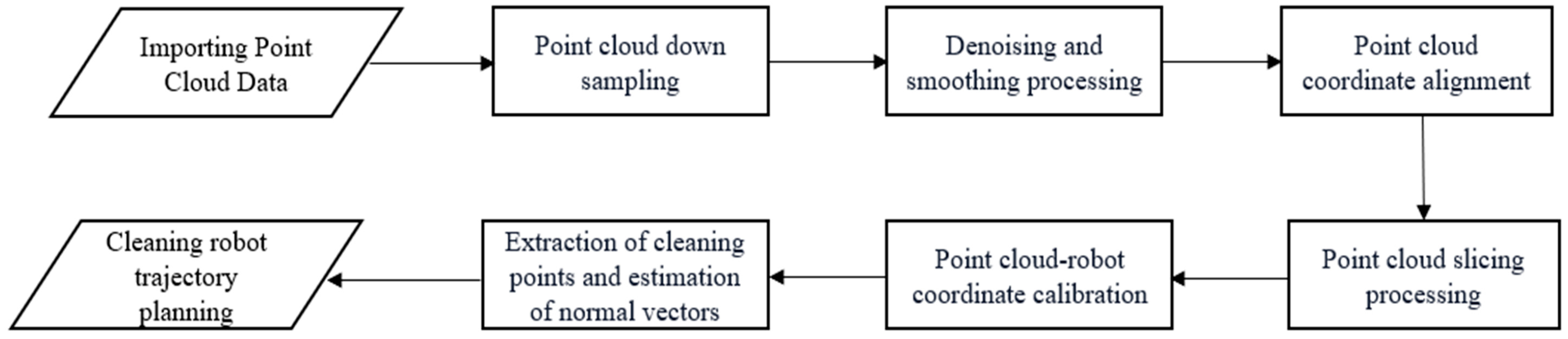
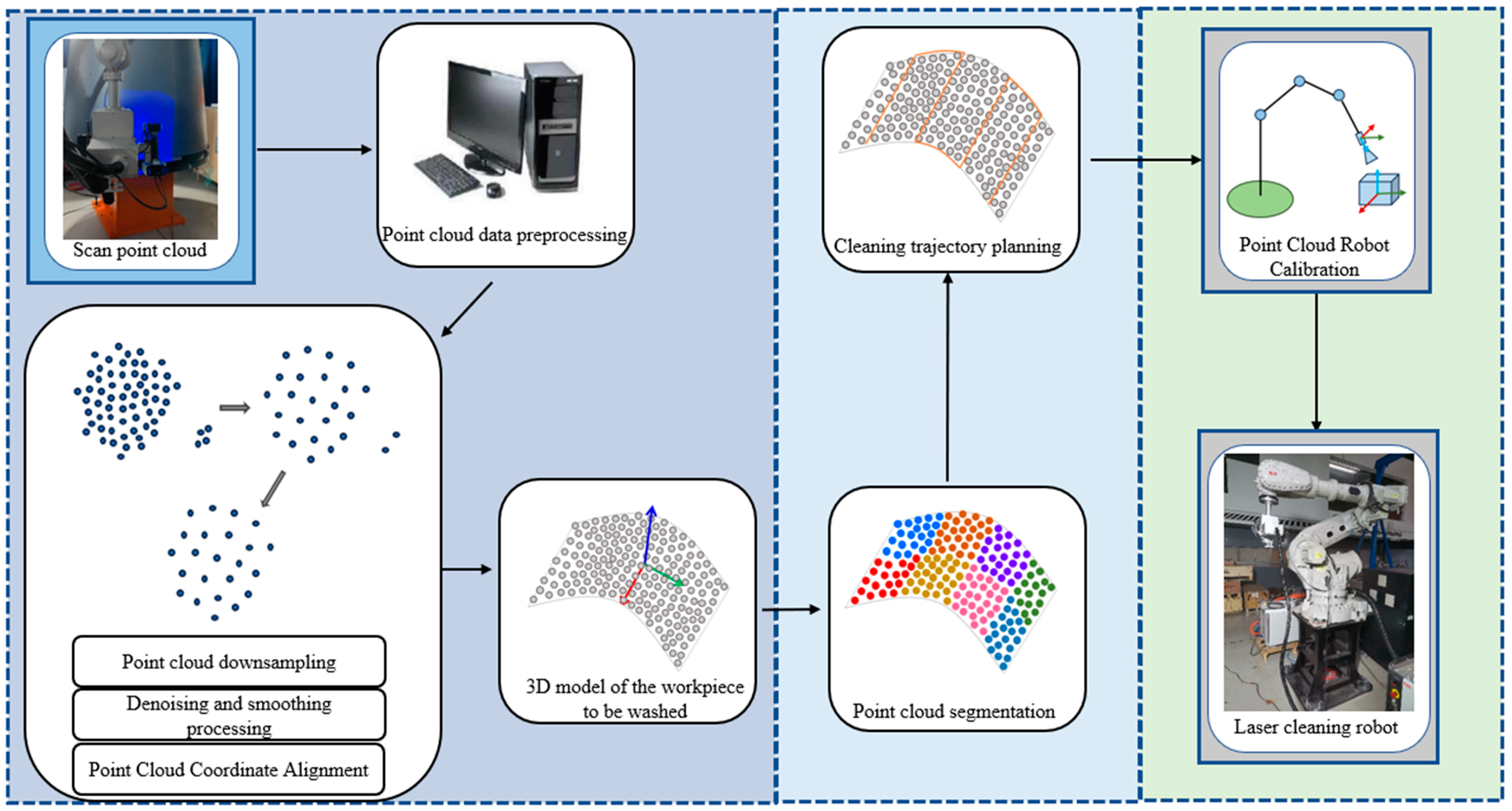
This section presents the development of an automated robot coating laser cleaning system by incorporating 3D sensors, robots, laser cleaning actuators, and computers. The system aims to achieve efficient and precise coating removal through automated laser cleaning. The flowchart of the laser cleaning trajectory planning algorithm is as shown in Figure 1, written using the C++ (c plus plus) programming language. The operational schematic of the system is shown in Figure 2.
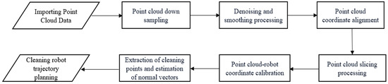
Figure 1.
Flow chart of the laser cleaning trajectory planning algorithm.

Figure 2.
Development of an automated robot coating laser cleaning system.
2.1.1. Measurement of Raw Point Cloud Data
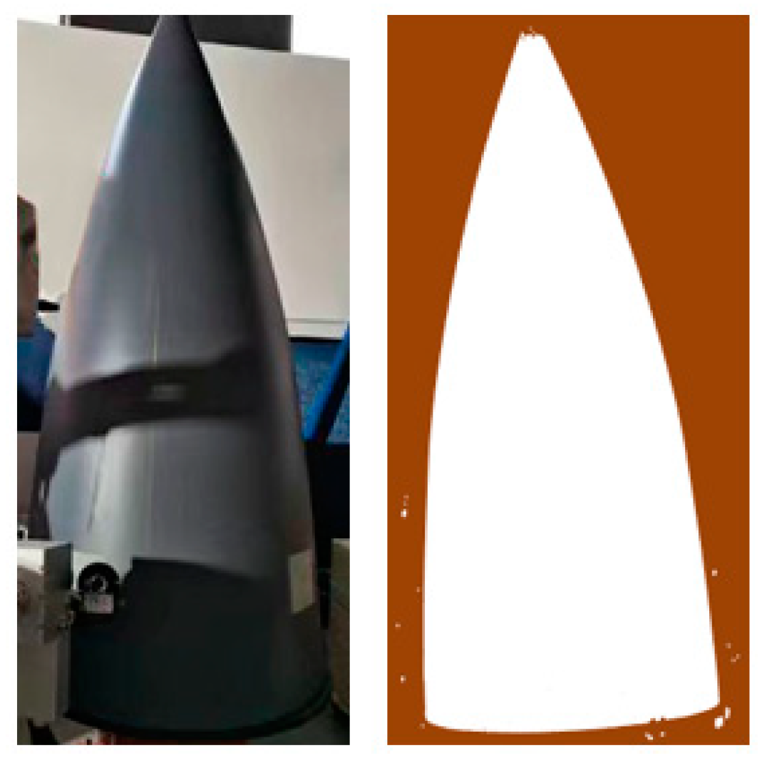
With the rapid development of 3D data acquisition technology, the utilization of 3D sensors for detecting the 3D profiles of objects has gained extensive application. In comparison to coordinate measuring machines (CMM) and articulated arm measuring machines, the advantages of 3D sensors are their non-contact measurement capability and wider detection range. In this study, measurements were performed using a 3D scanning sensor. Figure 3 presents a three-dimensional point cloud of an aircraft radome surface. The rotational symmetric radome was positioned with a base, as its vertical direction was aligned with the radome’s vertical axis.

Figure 3.
An aircraft radome and its 3D scanned point cloud of aircraft radome.
2.1.2. Point Cloud Data Preprocessing
During the acquisition of point cloud data on the surface of the aircraft radome, various factors may introduce disturbances. These factors include uneven lighting, vibrations, object occlusions, and aging of the scanning equipment, which could result in noise and voids in the point cloud data. Therefore, preprocessing the point cloud data becomes necessary to ensure its smoothness and uniformity. In order to handle the high-density point cloud data acquired by the 3D sensor, this study employed a voxel filtering method for down sampling [23]. It is a method that effectively reduces the number of data points while preserving the details of the point cloud. Additionally, a statistical filtering technique was employed to remove outliers in the down sampled point cloud [24]. For each point in the point cloud, its 50 nearest neighboring points (, , , ) are first determined. Subsequently, the Euclidean distance between the point and its neighboring points was calculated using the following formula:
where , and represent the coordinates of the points and along the x, y, and z axes, respectively. Next, for each point , the average distance to its 50 nearest neighboring points is calculated:
Additionally, the global average of the mean distances between all points and their neighboring points was calculated, resulting in two values, denoted as and .
here, represents the total number of points in the point cloud.
Lastly, a threshold value was set, where is a constant (in this paper, is set to 1). Any point with an average distance exceeding this threshold (i.e., > ) was considered an outlier and was removed from the point cloud. The radome point cloud shape after preprocessing is shown in Figure 4.

Figure 4.
Radome point cloud shape after preprocessing.
2.1.3. Point Cloud Data Alignment
After preprocessing, the point cloud shape of the aligned radome became evident. However, it was necessary to align the coordinates of measuring and cleaning systems before the segmentation of the radome point cloud. To solve this issue, this study introduced the principal component analysis (PCA) algorithm for aligning the point cloud data. Specifically, the research focuses on studying the orientation determination of the principal axis vectors for point cloud alignment. A PCA-based point cloud alignment algorithm was proposed, incorporating an additional criterion for determining the main direction. The algorithm’s specific steps for aligning the point cloud data are outlined as follows.
Firstly, decentralize the point cloud dataset :
The covariance matrix of dataset P can be calculated as:
Through eigenvalue decomposition calculation, the covariance matrix Eigenvalues and eigenvectors of can be expressed as:
where is a 3 × 3 matrix composed of the eigenvectors of the covariance matrix , used to identify the main directions of the point cloud data, and is a 3 × 3 diagonal matrix whose diagonal elements are the eigenvalues of the covariance matrix, indicating the variance of data in each direction.
Then a new O-XYZ right-hand coordinate system needed to be established. By taking the centroid coordinates as the origin of the new coordinate system, the first principal component of the eigenvector corresponding to the maximum eigenvalue was chosen as the X-axis of the new coordinate system. The second principal component of the eigenvector corresponding to the second largest eigenvalue was chosen as the Y-axis of the new coordinate system. Thereby, the O-XY plane was formed. By performing a cross-product operation on the X-axis and Y-axis, the new Z-axis coordinate was obtained and the new O-XYZ coordinate system was established.
By utilizing the newly constructed O-XYZ coordinate system, the coordinate transformation matrix dataset could be computed to obtain the axis-aligned set .
where is the rotation matrix and is the translation vector.
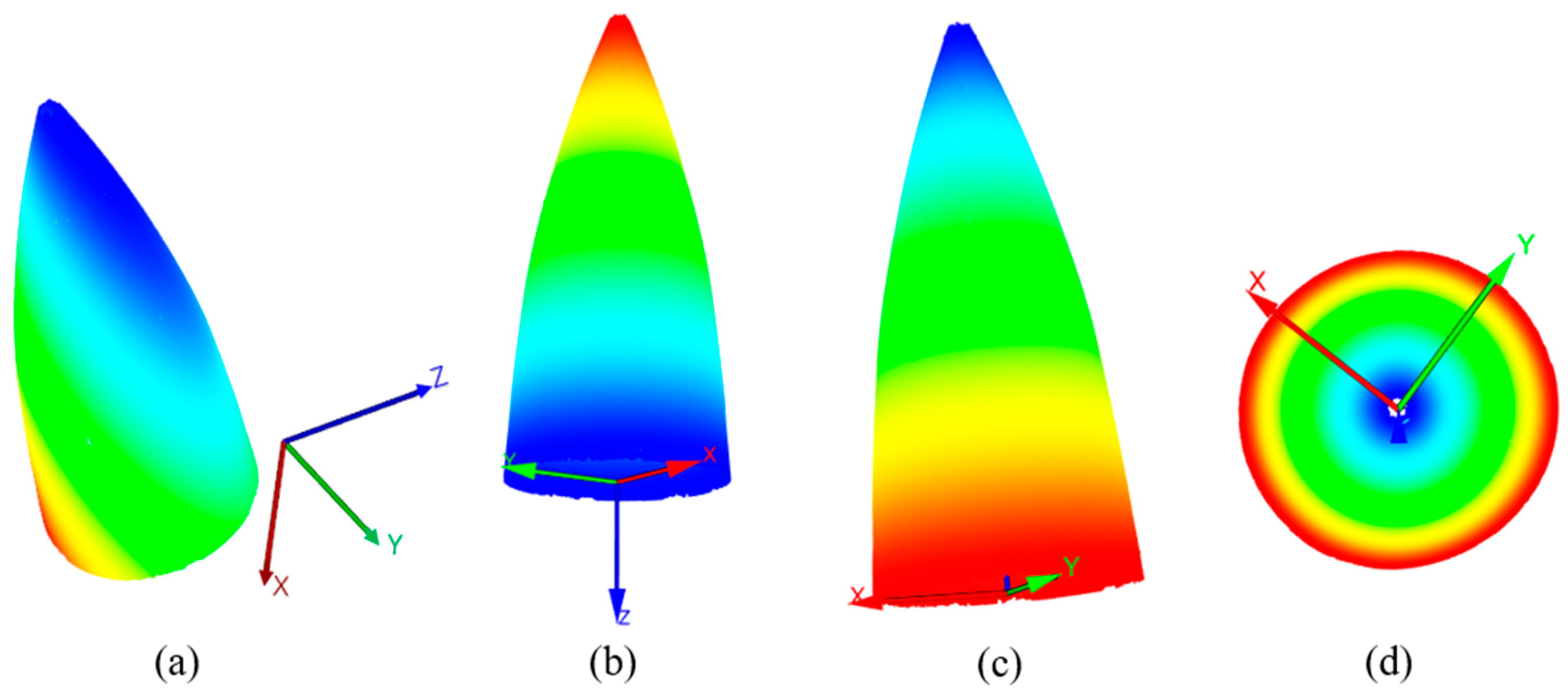
There may exist a problem with the Z-axis orientation, resulting in a scenario where the aligned point cloud exhibits an inverted orientation as depicted in Figure 5b. Specifically, when the Z-component values of the point cloud data are negative, it indicates a reversal in the Z-axis direction. Consequently, after the initial alignment of the point cloud coordinate system, it was necessary to perform Z-axis direction determination and correction.

Figure 5.
Alignment of radar hood point cloud coordinates (Z-axis rendering): (a) radar hood point cloud before coordinate alignment, (b) radar hood point cloud after initial alignment, (c) radar hood point cloud aligned through Z-axis correction, and (d) bottom-up view of the radar hood point cloud after alignment.
We needed to search for the maximum point and the minimum point in the point cloud set . Extract the corresponding Z-axis component values and , respectively. Take the absolute values of and and calculate their difference as shown in Equation (10). From the perspective of the point cloud data, this step involves comparing the maximum and minimum points of the point cloud set to determine if the Z-axis is reversed.
Based on the value obtained in Equation (10), denoted as m, if m is determined to be negative, it indicates that the Z-axis is reversed. In such cases, a Z-axis correction is required, as shown in Equation (11), resulting in the aligned point cloud set . Figure 5b illustrates the initial alignment of the point cloud and the Z-axis direction correction, leading to the aligned point cloud depicted in Figure 5c.
where .
2.2. Slicing and Visualization of Radome Point Cloud Data
2.2.1. Radome Point Cloud Data Slicing Processing
After repositioning the point cloud coordinate system at the origin, it was necessary to consider slicing the radar hood point cloud model. Due to the inherent geometric characteristics of the radar hood, vertical slicing was performed first based on its height symmetry, followed by horizontal slicing. Considering the complexity of horizontally slicing the radar hood point cloud model in three-dimensional space, a projection-based point cloud slicing technique was proposed. This technique enables rapid and accurate horizontal segmentation of the radar hood point cloud model.
Slicing in the Z-Axis Direction
The radar hood point cloud model was divided into several layers based on the z-coordinate. The division was determined by the laser cleaning range, denoted as h, and took into account an angle (The choice of was dictated by factors such as the physical structure of the radar hood and the positioning of the cleaning equipment.) The height of each layer was calculated as . For a radar hood with a height of H, it was divided into sections. The height at which each layer’s slicing line was located was denoted as . The point cloud was sorted in ascending order based on the z-coordinate, and each point was assigned to the corresponding layer based on its z-coordinate value.
Projection-Based Point Cloud Segmentation for Radar Hood Geometry
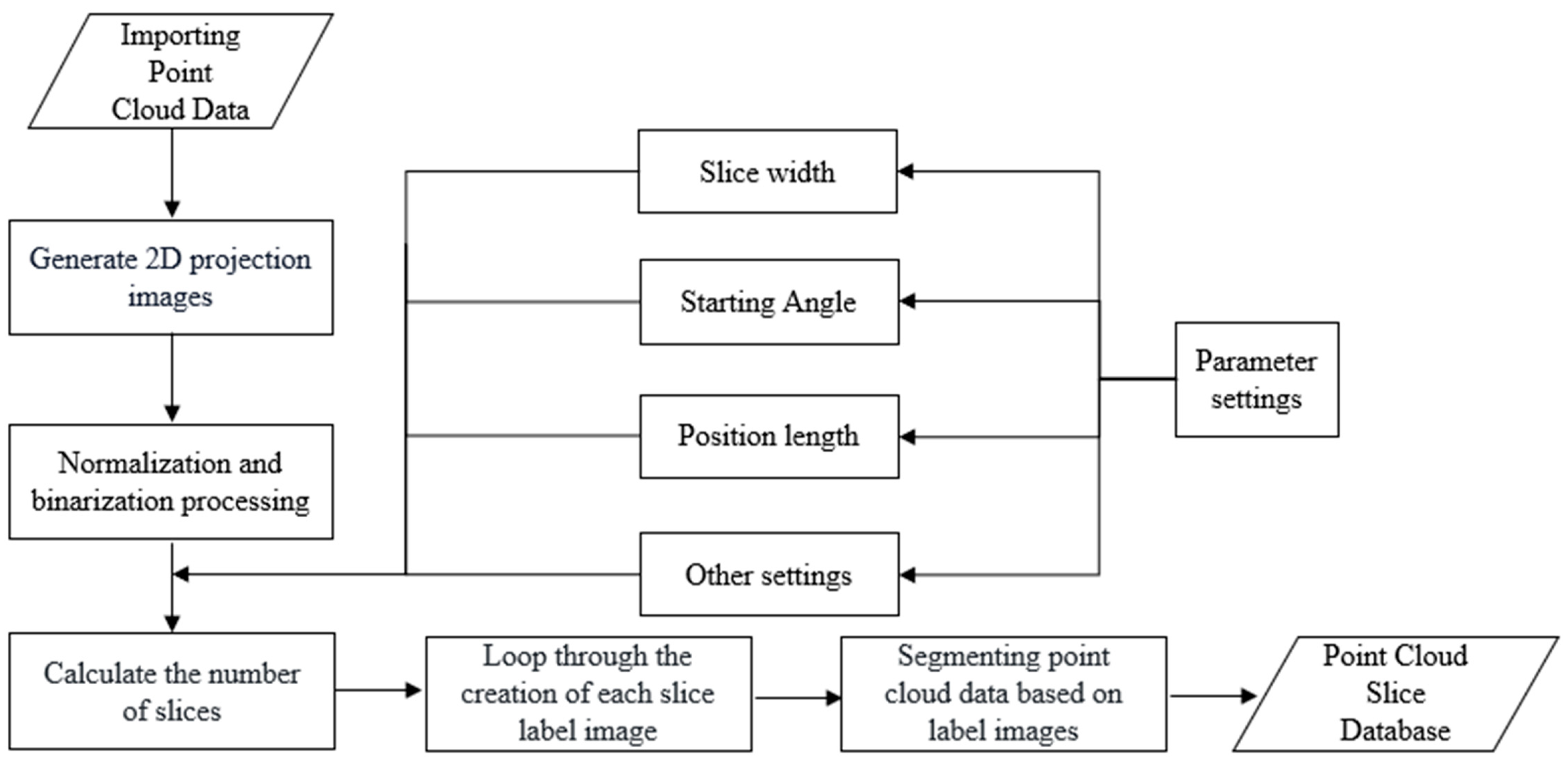
Considering the geometric characteristics of radar domes, the annular structure formed after height segmentation requires further horizontal segmentation. The projection-based point cloud segmentation technique is a method that projects the point cloud onto a 2D space for processing, aiming to reduce the complexity of horizontal slicing of the point cloud. The algorithm flow of this technique is illustrated in Figure 6.
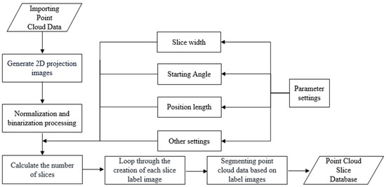
Figure 6.
Projection-based point cloud segmentation process.
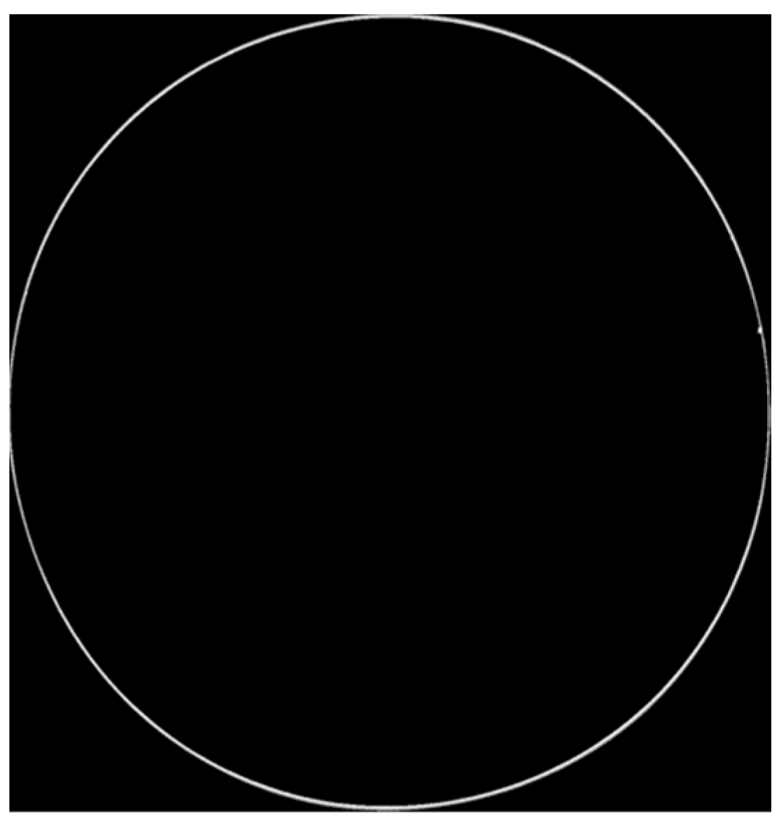
The point cloud of the radar radome was projected onto the Z-direction and underwent normalization and binarization after height segmentation. By extracting the contour of the binarized image, the annular segments of the radar dome were obtained, as shown in Figure 7. Based on the horizontal scanning range of the laser, the segmentation dimensions were calculated and the radar dome was horizontally segmented into annular sections. The circumference of each radar dome ring was denoted as W, the horizontal cleaning range as w, the angle of the ring as , and the number of segmentations within the ring as M. Thus, . After partitioning, each segmentation line was assigned an angle . The regions within each ring were assigned corresponding pixel values based on the magnitude of . An image with the same size as the binarized image was initialized, with all pixel values set to 0, referred to as the label image. In each segmented region of the ring, the positions of non-zero pixels within the current region were identified and the corresponding pixel values in the label image were set to the current label value. Using the label image obtained, the current original point cloud data within the segmented ring were labeled, cached, and fused, with the point cloud list being promptly updated. Upon traversing all the layers of points, the data were saved into the point cloud segmentation database, resulting in a collection of point cloud slices, denoted as S .
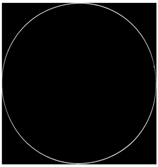
Figure 7.
Projection of height-segmented image.
2.2.2. Visualization of Projected Slices
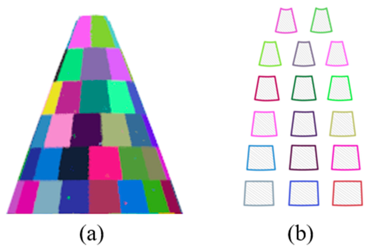
In terms of visualizing the sliced data of the radar dome point cloud, this study utilized the visualization tool based on PCL (Point Cloud Library). Prior to visualization, the radar dome point cloud model was segmented along the z-axis and the horizontal direction, with each slice sequentially stored in the collection S. Each slice was indexed based on the slicing order and assigned a unique RGB color to ensure color uniqueness and consistency. Figure 8 illustrates the unfolded view of the radar dome point cloud data slices, which facilitates a clearer observation and analysis of the sliced data.

Figure 8.
Splitting expansion of radome point cloud data: (a) top model segmentation of radome and (b) expanded slice data.
2.3. Laser Cleaning Robot Trajectory Planning
The trajectory of the robot should be generated prior to the laser coating cleaning process. To achieve optimal cleaning results, two principles must be followed:
(1) The trajectory of the robot for laser coating cleaning should align with the surface height of the component to be cleaned;
(2) The central axis of the laser cleaning actuator held by the robot should always be perpendicular to the surface of the workpiece.
2.3.1. Calibration of Coordinate Relationship between Radome Measurement Point Cloud and Cleaning Robot
The aligned point cloud coordinate system differs from the robot coordinate system. In this study, a homogeneous transformation matrix was employed to perform the transformation from the point cloud coordinate system to the robot coordinate system. The transformation matrix was defined as follows:
where R is a 3 × 3 rotation matrix and t is the translation vector.
2.3.2. Calculation Model for Laser Cleaning Actuator Point Coordinates
Geometric Relationship Model between Cleaning Actuator Points and Sliced Point Cloud
The definition of the laser coating cleaning actuator point is the central point of the effective processing area of the laser spot during a single cleaning operation. In a single cleaning operation, the laser cleaning device can achieve comprehensive coverage and cleaning of the effective processing area. Therefore, all points within this area can be simplified to a single cleaning point, represented by the centroid of the point cloud slice. The calculation formula for this point is as follows:
Among them, the set of slice points is . Store the cleaning point data in the point set ListU.
The Estimation of the Normal Vector for the Cleaning Points
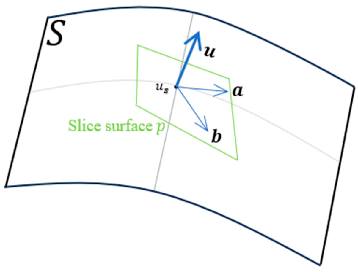
For a regular surface S in three-dimensional space, the normal vector u at point can be approximated as the normal vector of the surface at point . In the tangent plane p at , vectors a and b are two non-collinear vectors, as shown in Figure 9.
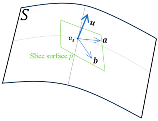
Figure 9.
Illustration of point cloud normal vector estimation.
The data stored in ListU consist of a series of points, forming a sampling point set U. The normal vector at each data point in the sampling point set represents the normal vector of the local tangent plane at that point on the surface. There are two main methods for estimating the normal vectors. One method involves the scattered data’s triangulated topology, where the normal vector is obtained from the normal vectors of the relevant triangles in the point cloud data, considering the triangulated topology of the point cloud data. The other method utilizes the neighborhood information of each point and employs the least squares principle to locally fit a plane to the K neighboring points. The fitted plane can be considered as the local tangent plane at that point. The normal vector of the local tangent plane at that point is then regarded as the normal vector of the sampling point. This method provides better flexibility by adjusting the neighborhood size to balance the smoothness and details of the normal vectors. The following formula is used to calculate the plane fitting for each point’s K neighborhood:
where represents the normal vector of the locally fitted plane , while denotes the k neighboring points of within . The variable d represents the distance from the fitted plane to the origin of the coordinate system.
The normal vector of plane is determined through principal component analysis (PCA), by analyzing the eigenvector corresponding to the minimum eigenvalue of the covariance matrix . This minimum eigenvector represents the normal vector of plane . The covariance matrix is defined as follows:
where denotes the centroid of the k neighborhood points around point .
To fit the plane , satisfying the condition of minimizing the sum of squared distances between the neighboring points and the plane, we utilized the Lagrange theorem to solve the covariance matrix A and the plane’s normal vector, , which satisfied the following relationship:
where λ represents the eigenvalues of matrix A. When λ reaches its minimum value, the corresponding vector is the normal vector of the fitted plane , which can be approximated as the normal vector of point , denoted as .
The direction of the normal vector can be determined using the viewpoint method. Let us consider a point q within the object under inspection. If the relationship between and q satisfies Equation (17), then the direction of the normal vector remains unchanged. However, if the relationship does not hold, the direction of the normal vector is reversed to ensure uniformity in the direction of the normal vectors.
where is the normal vector of point q.
2.3.3. Execute Point Fitting to Generate Cleaning Robot Trajectory
Discrete Point Fitting for Generating Cleaning Robot Trajectory
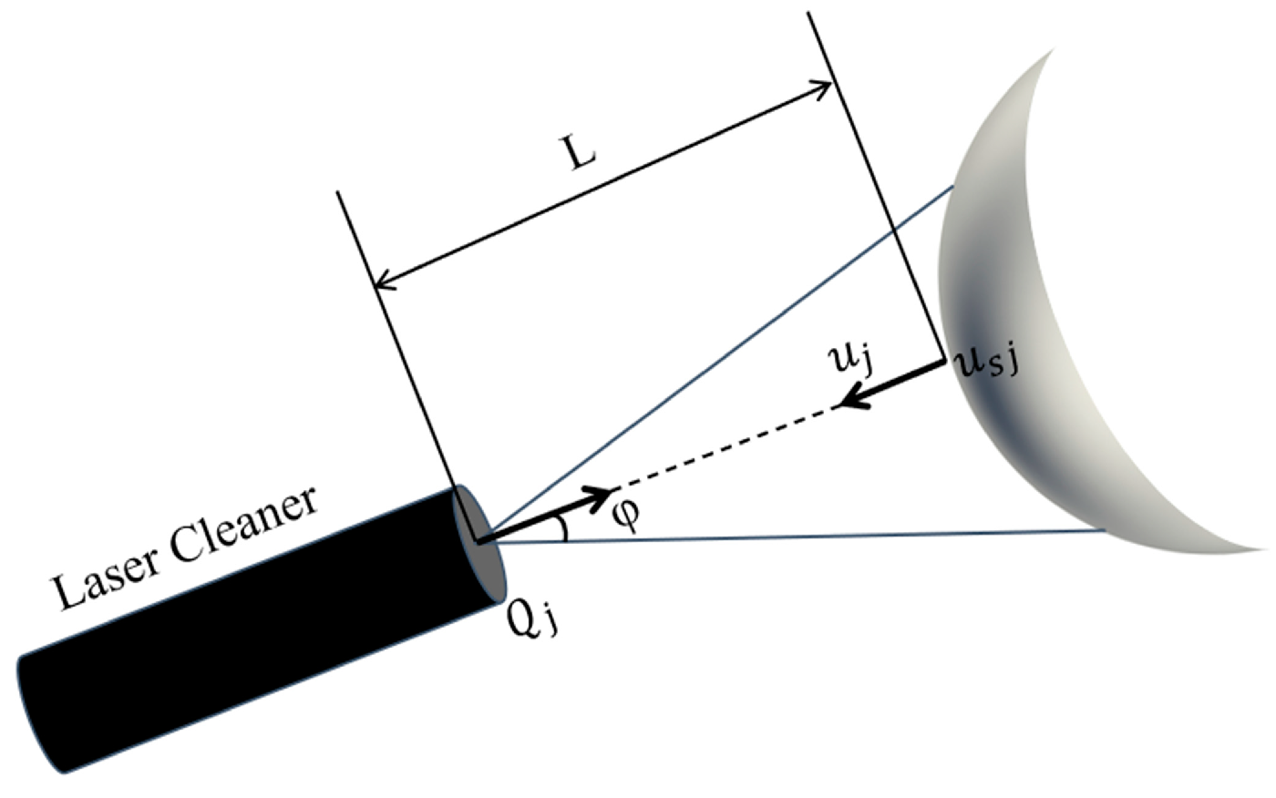
In accordance with the requirements of laser cleaning tasks performed by the cleaning robot, the vertical distance from the laser cleaning actuator to the surface of the target workpiece was denoted as L. The trajectory parameters of the laser cleaning actuator can be obtained using the following offset algorithm:
As shown in Figure 10, the point includes the position (coordinate values) and directional information (opposite to the direction of ) of the end effector of the laser cleaning actuator.
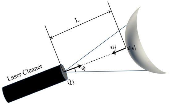
Figure 10.
The position and direction of the laser cleaner at point .
To obtain the offset point set Q, a similar method was applied to traverse all points in the sampling point set R. Consequently, the information contained in the entire point set Q represented the trajectory parameters (position and direction) of the laser cleaning device on the operating surface during the cleaning process.
B-spline curves are derived from the basis of Bézier curves, which were introduced by Schoenberg in the 1940s [25] and later formulated recursively by De Boor [26,27] and Cox [28]. The recursive nature of B-spline curves makes the computation straightforward and stable, leading to widespread adoption. These curves are generated by combining control points with B-spline basis functions to define the shape of the curve. In this paper, B-splines were employed for curve fitting purposes. The mathematical expression for a pth-degree B-spline curve is given by Equation (19). By connecting the respective execution points, a continuous path was formed, which can be transformed into a specific model of laser cleaning robot’s motion program. This enabled automated laser cleaning of the workpiece surface for coating removal.
where represents the degree of the spline curve and denotes the control points of the curve.
The control polygon, formed by connecting the control points in a specific order, is referred to as the control polygon of the curve. Typically, the parameter values and are used. represents the basis function of a pth-degree B-spline curve, as given by Equation (21), which is defined as a piecewise polynomial function determined by the knot vector . The knot vector is a non-decreasing sequence composed of all the knots. In B-spline curves, the first and last control points are typically used as the start and end points of the curve, while the intermediate control points serve as the breakpoints or knots of the curve. To ensure that the pth-degree spline curve passes through the first and last control points, the first and last knots are repeated p+1 times. In this paper, the knot vector was parameterized using the cumulative chord length method, as shown in Equation (20).
where represents the normalized chord length vector.
where the number of control points are ), the degree of the spline curve () and the number of knots satisfies . Once the degree () and the knot vector () are determined, the basis functions of the B-spline curve can be computed.
Hierarchical Smooth Transition of Motion Trajectories
During laser cleaning processes, it is crucial for the robot to achieve smooth transitions between different cleaning levels. By employing B-spline curve fitting, discrete cleaning execution points have been successfully transformed into continuous path planning. However, it is necessary to ensure smooth and appropriate transitions between these paths at different levels, reducing trajectory discontinuities when switching between levels, thus ensuring stability and efficiency in the cleaning process.
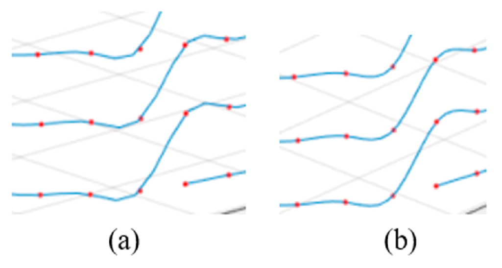
Between the endpoints of each level and the starting points of the next level, the adjustment of control points in B-spline curves enables achieving consistent first-order derivatives at the connecting points of two different levels. This optimization of the connection path ensures smoothness, as shown in Equation (22). When the first-order derivatives at the connecting points of two different-level curves are equal, it indicates continuity in the tangent direction at those points. Figure 11 provides a comparative illustration, demonstrating the difference between connecting points of two different-level curves with and without the implementation of the first-order derivative consistency constraint. This approach helps avoid abrupt changes in angles at the path connections, ensuring smoother and more natural robot motion.
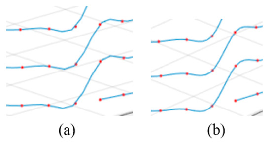
Figure 11.
Comparative illustration of connecting points of two different-level curves. (a) Connecting points of two curves without the constraint of first-order derivative consistency. (b) Connecting points of two curves with the constraint of first-order derivative consistency.
In the equations, represents the first derivatives of the curve at point d. and are the parameter values at the connection points of adjacent level paths.
During the robot’s transition between levels, it is essential to reduce its motion speed appropriately to avoid mechanical arm vibrations and posture deviations caused by rapid movements. Moreover, adjustments to the robot’s posture are necessary to maintain an appropriate distance and angle between the laser cleaning head and the workpiece surface. This helps decrease mechanical wear and the potential risks of malfunctions resulting from improper motion.
3. Results
The remote-control system hardware used in the experiment consists of an ABB (Asea Brown Boveri) IRB (Industrial Robot) series 6700 robot, a control cabinet, and a computer. The computer communicates with the control cabinet using the RAPID language in RobotStudio software, which controls the robot’s motion. The host computer, running laser cleaning software on the Windows operating system, acts as the main control system. It establishes communication and connection with the ABB robot through the Internet options or TCP/IP protocol of the robot’s PC. Additionally, it connects and communicates with the Siemens 1200 series PLC via Ethernet or other communication methods to control the robot system and laser system and monitor device status. Offline trajectory planning is performed on the 3D point cloud, which offers more freedom and accurate trajectory planning compared to online programming in RobotStudio software.
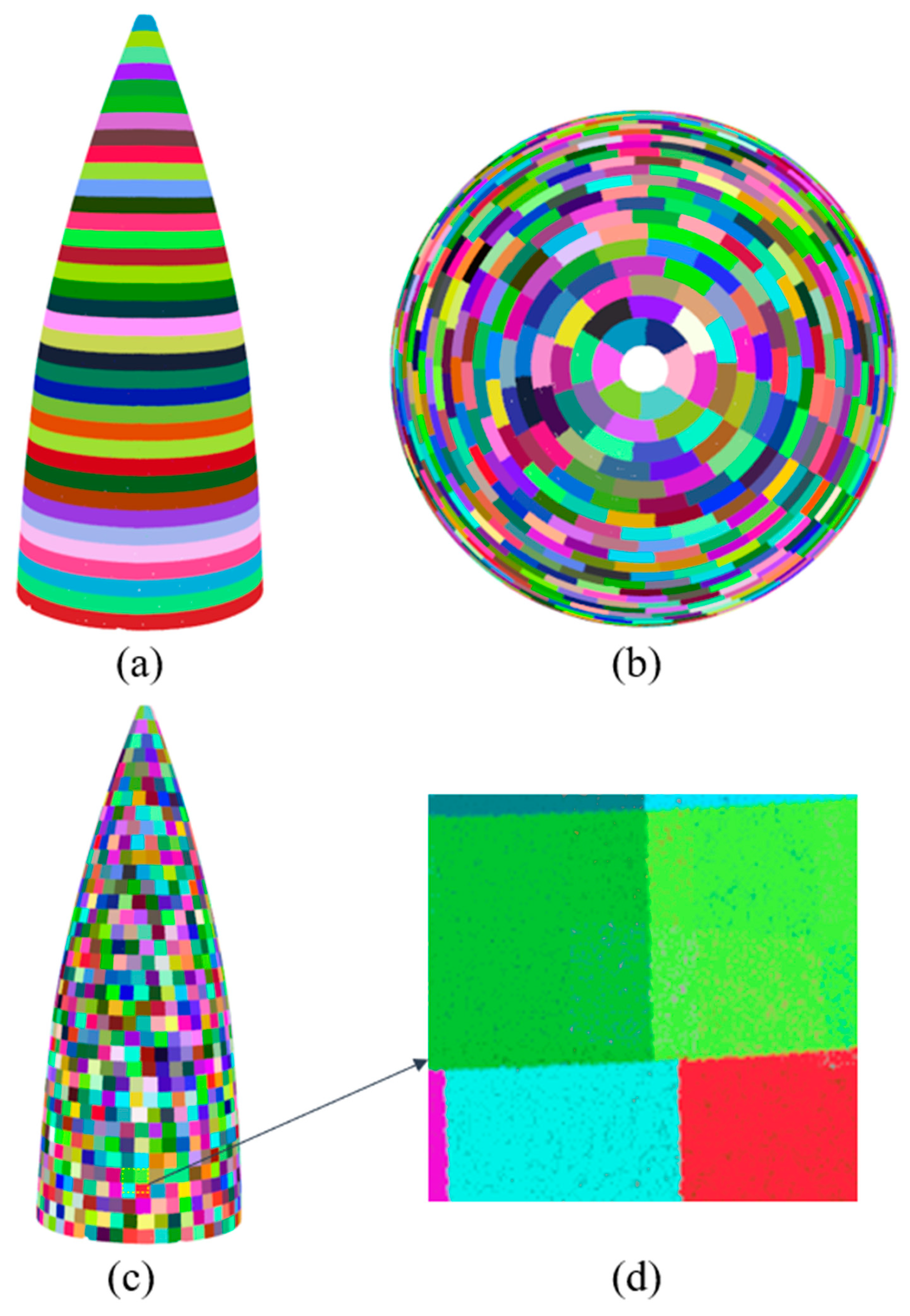
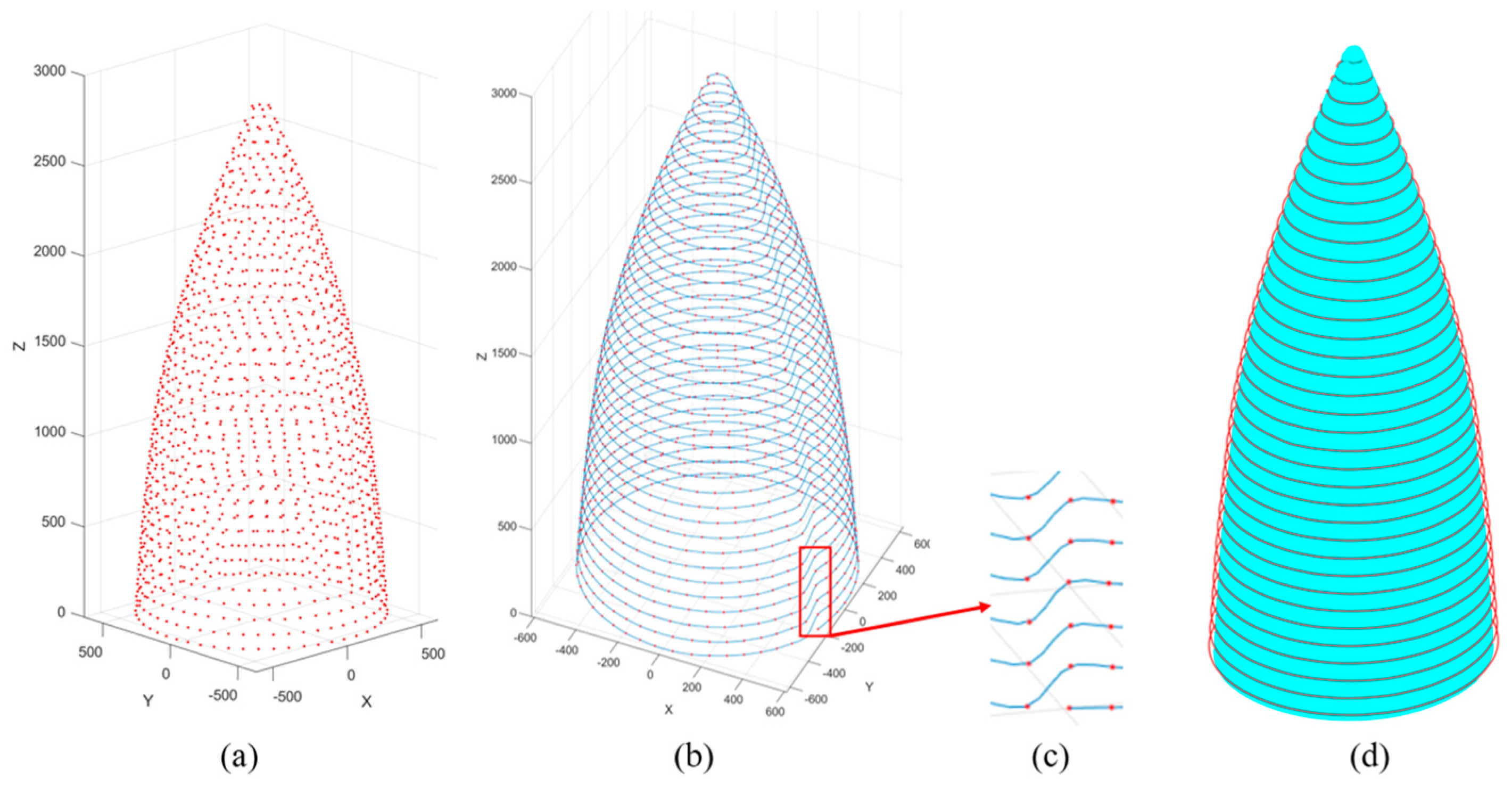
In this study, a radar dome of an aircraft was chosen as the experimental object. A 3D scanner was used to scan the radar dome and obtain point cloud data. The point cloud data were then preprocessed and aligned to generate a 3D model of the radar dome’s surface. This model was imported into the offline programming software, and based on the surface curvature of the radar dome, limitations of the laser cleaning area, and focal depth requirements (in this experiment, the angle is 36.87 degrees), the surface of the radar dome was divided into regions, as shown in Figure 12.
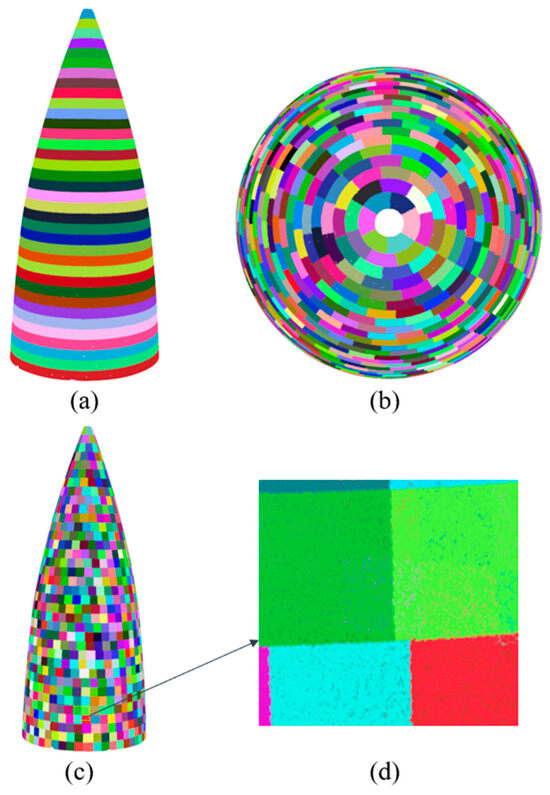
Figure 12.
Radome point cloud model segmentation: (a) vertical segmentation effect of point cloud, (b) top view after point cloud segmentation, (c) horizontal segmentation effect of point cloud, and (d) local segmentation effect of point cloud segmentation.
By employing a point cloud segmentation algorithm, a series of slices were generated, as shown in Figure 12c. For each slice, a centroid calculation was performed to extract the cleansing positions of the radar radome, as shown in Figure 13a. In Figure 14a, an estimation of the normal vectors at the extracted cleaning points is presented, and numerical annotations within the figure denote the sequence of the motion trajectory during the laser cleaning process. Leveraging the B-spline curve fitting method and hierarchical stitching processing, the spatial trajectory of the laser cleaning robot was obtained, as shown in Figure 13b.

Figure 13.
Execution point fitting generates cleaning robot trajectory: (a) extracted cleaning point positions, (b) trajectory planning for robot laser cleaning, (c) local enlarged layered connections, and (d) cleaning the movement trajectory of the robot.
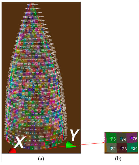
Figure 14.
Estimation of normal vector for cleaning point location: (a) normal vector for cleaning execution point and (b) local enlarged display.
Before trajectory planning for laser cleaning by the robot, it was necessary to perform point cloud-to-robot calibration, which involves transforming the coordinate system of the radar radome point cloud to that of the robot. To achieve this problem, point selection calibration between the point cloud and the robot was carried out. In order to improve accuracy, a total of 10 data sets was collected and the homogeneous transformation matrix for the point cloud-to-robot calibration was computed. The computed transformation matrix is shown below.
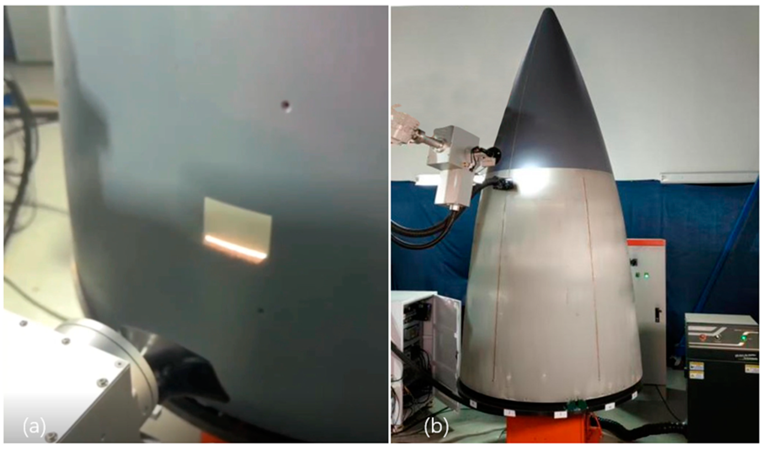
To illustrate the practicality of the proposed method in real-world scenarios, a surface coating laser cleaning was conducted on an actual radar radome. Prior to the execution of the cleaning trials, it was imperative to fine-tune the laser cleaning parameters on a test piece composed of identical material to guarantee the attainment of thorough cleanliness in a solitary scan. The parameters for laser cleaning are delineated in Table 1. The system employs a pulsed fiber laser, characterized by a central wavelength of 1064 nm, a circular core diameter of 400 um, and a maximum output power of 1000 W. Figure 15 provides a clear demonstration of the effectiveness of laser cleaning. The efficiency of this robotic laser cleaning system was determined by calculating the ratio of cleaning duration to the area cleaned, yielding a cleaning efficiency of 2.94 . This represents a significant improvement over the efficiency of 0.396 m2/h reported in [29], thereby highlighting a marked enhancement in performance metrics. The trajectory planning method mentioned successfully removed the coating from the test section, meeting the experimental requirements.

Table 1.
Laser cleaning parameters.
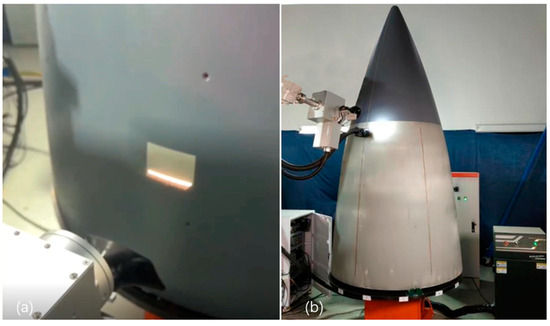
Figure 15.
Laser cleaning: (a) the cleaning of a slice of workpieces and (b) the movement of the laser cleaning head between different slice layers.
4. Conclusions and Discussion
This research developed a path-planning method for the shape-following laser cleaning automated robot of aircraft radar coating. The proposed method enables accurate cleaning of coating on the radar without known surface equations or CAD models. Through the aircraft radar radome laser cleaning experiments, the effectiveness of the proposed method was validated. The final cleaning results demonstrate the wide potential and high cleaning efficiency in industrial applications.
Author Contributions
Conceptualization, Z.Z. (Zhen Zeng) and C.J.; methodology, C.J. and Z.Z. (Zhen Zeng); software, S.D., Q.L. and C.J.; validation, Z.Z. (Zhongsheng Zhai), S.D. and C.J.; formal analysis, Z.Z. (Zhen Zeng) and C.J.; investigation, Z.Z. (Zhongsheng Zhai); resources, S.D., D.C. and C.J.; data curation, Z.Z. (Zhongsheng Zhai) and S.D.; writing—original draft preparation, Z.Z. (Zhen Zeng) and C.J.; writing—review and editing, Z.Z. (Zhongsheng Zhai) and S.D.; visualization, Z.Z. (Zhen Zeng); supervision, S.D. and Q.L.; project administration, Z.Z. (Zhongsheng Zhai) and D.C.; funding acquisition, Z.Z. (Zhongsheng Zhai). All authors have read and agreed to the published version of the manuscript.
Funding
This research was funded by the Hubei Natural Science Foundation (No. 2022CFA006), and the Wuhan Key Research and Development Plan (No. 2022012202015034).
Institutional Review Board Statement
Not applicable.
Informed Consent Statement
Not applicable.
Data Availability Statement
The raw data supporting the conclusions of this article will be made available by the authors on request.
Conflicts of Interest
The authors declare no conflict of interest.
References
- Bertasa, M.; Korenberg, C. Successes and challenges in laser cleaning metal artefacts: A review. J. Cult. Herit. 2022, 53, 100–117. [Google Scholar] [CrossRef]
- Razab, M.K.A.A.; Jaafar, M.S.; Abdullah, N.H.; Suhaimi, F.M.; Mohamed, M.; Adam, N.; Yusuf, N.A.A.N.; Noor, A.M. A review of incorporating Nd:YAG laser cleaning principal in automotive industry. J. Radiat. Res. Appl. Sci. 2018, 11, 393–402. [Google Scholar] [CrossRef]
- Li, X.; Huang, T.; Chong, A.W.; Zhou, R.; Choo, Y.S.; Hong, M. Laser cleaning of steel structure surface for paint removal and repaint adhesion. Opto-Electron. Eng. 2017, 44, 340–344. [Google Scholar]
- Zhang, G.; Hua, X.; Huang, Y.; Zhang, Y.; Li, F.; Shen, C.; Cheng, J. Investigation on mechanism of oxide removal and plasma behavior during laser cleaning on aluminum alloy. Appl. Surf. Sci. 2020, 506, 144666. [Google Scholar] [CrossRef]
- Li, Z.; Zhang, D.; Su, X.; Yang, S.; Xu, J.; Ma, R.; Shan, D.; Guo, B. Removal mechanism of surface cleaning on TA15 titanium alloy using nanosecond pulsed laser. Opt. Laser Technol. 2021, 139, 106998. [Google Scholar] [CrossRef]
- Zhu, G.; Xu, Z.; Jin, Y.; Chen, X.; Yang, L.; Xu, J.; Shan, D.; Chen, Y.; Guo, B. Mechanism and application of laser cleaning: A review. Opt. Lasers Eng. 2022, 157, 107130. [Google Scholar] [CrossRef]
- Ding, K.; Zhou, K.; Feng, G.; Han, J.; Xie, N.; Huang, Z.; Zhou, G. Mechanism and conditions for laser cleaning of micro and nanoparticles on the surface of transparent substrate. Vacuum 2022, 200, 110987. [Google Scholar] [CrossRef]
- Zhao, H.; Qiao, Y.; Du, X.; Wang, S.; Zhang, Q.; Zang, Y.; Liu, X. Laser cleaning performance and mechanism in stripping of Polyacrylate resin paint. Appl. Phys. A 2020, 126, 360. [Google Scholar] [CrossRef]
- Vorobyev, A.Y.; Guo, C. Residual thermal effects in laser ablation of metals. J. Phys. Conf. Ser. Eighth Int. Conf. Laser Ablation 2017, 59, 418–423. [Google Scholar] [CrossRef]
- Li, X.; Zhang, Q.; Zhou, X.; Zhu, D.; Liu, Q. The influence of nanosecond laser pulse energy density for paint removal. Optik 2018, 156, 841–846. [Google Scholar] [CrossRef]
- Bykanova, A.Y.; Kostenko, V.V.; Tolstonogov, A.Y. Development of the underwater robotics complex for laser cleaning of ships from biofouling: Experimental results. IOP Conf. Ser. Earth Environ. Sci. 2020, 459, 032061. [Google Scholar] [CrossRef]
- Zhu, G.; Shi, S.; Fu, G.; Shi, J.; Yang, S.; Meng, W.; Jiang, F. The influence of the substrate-inclined angle on the section size of laser cladding layers based on robot with the inside-beam powder feeding. Int. J. Adv. Manuf. Technol. 2017, 88, 2163–2168. [Google Scholar] [CrossRef]
- De Graaf, M.; Aarts, R.; Jonker, B.; Meijer, J. Real-time seam tracking for robotic laser welding using trajectory-based control. Control Eng. Pract. 2010, 18, 944–953. [Google Scholar] [CrossRef]
- Wei, W.; Chao, Y.U.N. A path planning method for robotic belt surface grinding. Chin. J. Aeronaut. 2011, 24, 520–526. [Google Scholar]
- Bian, Y.; Zhang, Y.; Gao, Z. A path planning method of robotic belt grinding system for grinding workpieces with complex shape surfaces. In Proceedings of the International Conference on Emerging Trends in Engineering and Technology (ICETET), Phuket, Thailand, 7–8 December 2013. [Google Scholar]
- Cai, Z.; Liang, H.; Quan, S.; Deng, S.; Zeng, C.; Zhang, F. Computer-aided robot trajectory auto-generation strategy in thermal spraying. J. Therm. Spray Technol. 2015, 24, 1235–1245. [Google Scholar] [CrossRef]
- Morozov, M.; Pierce, S.G.; MacLeod, C.N.; Mineo, C.; Summan, R. Off-line scan path planning for robotic NDT. Measurement 2018, 122, 284–290. [Google Scholar] [CrossRef]
- Geng, Y.; Zhang, Y.; Tian, X.; Shi, X.; Wang, X.; Cui, Y. A novel welding path planning method based on point cloud for robotic welding of impeller blades. Int. J. Adv. Manuf. Technol. 2022, 119, 8025–8038. [Google Scholar] [CrossRef]
- Zhang, Z.; Zhang, H.; Yu, X.; Deng, Y.; Chen, Z. Robotic trajectory planning for non-destructive testing based on surface 3D point cloud data. J. Phys. Conf. Ser. 2021, 1965, 012148. [Google Scholar] [CrossRef]
- Hu, D.; Gan, V.J.L.; Wang, T.; Ma, L. Multi-agent robotic system (MARS) for UAV-UGV path planning and automatic sensory data collection in cluttered environments. Build. Environ. 2022, 221, 109349. [Google Scholar] [CrossRef]
- Ye, X.; Luo, L.; Hou, L.; Duan, Y.; Wu, Y. Laser ablation manipulator coverage path planning method based on an improved ant colony algorithm. Appl. Sci. 2020, 10, 8641. [Google Scholar] [CrossRef]
- Shuo, J.; Yuan, R.; Qingzeng, M.; Hailong, G.; Wenlong, L.; Wei, C. Off-line programming of robot on laser cleaning for large complex components. J. Phys. Conf. Ser. 2021, 1748, 022027. [Google Scholar] [CrossRef]
- Miknis, M.; Davies, R.; Plassmann, P.; Ware, A. Efficient point cloud pre-processing using the point cloud library. Int. J. Image Process. 2016, 10, 63. [Google Scholar]
- Gordon, W.J.; Riesenfeld, R.F. B-spline curves and surfaces. In Computer Aided Geometric Design; Academic Press: Cambridge, MA, USA, 1974; pp. 95–126. [Google Scholar]
- Schoenberg, I.J. Contributions to the problem of approximation of equidistant data by analytic functions. Part B. On the problem of osculatory interpolation. A second class of analytic approximation formulae. Q. Appl. Math. 1946, 4, 112–141. [Google Scholar] [CrossRef]
- De Boor, C. On calculating with B-splines. J. Approx. Theory 1972, 6, 50–62. [Google Scholar] [CrossRef]
- De Boor, C. A Practical Guide to Splines; Springer: New York, NY, USA, 1978. [Google Scholar]
- Cox, M.G. The numerical evaluation of B-splines. IMA J. Appl. Math. 1972, 10, 134–149. [Google Scholar] [CrossRef]
- Pan, C.Q.; Zhu, X.W.; Yang, W.F. Design of robotic laser shape-follow cleaning control system for large freeform surface workpiece. Appl. Laser 2021, 41, 1280–1286. [Google Scholar]


Disclaimer/Publisher’s Note: The statements, opinions and data contained in all publications are solely those of the individual author(s) and contributor(s) and not of MDPI and/or the editor(s). MDPI and/or the editor(s) disclaim responsibility for any injury to people or property resulting from any ideas, methods, instructions or products referred to in the content. |
© 2024 by the authors. Licensee MDPI, Basel, Switzerland. This article is an open access article distributed under the terms and conditions of the Creative Commons Attribution (CC BY) license (https://creativecommons.org/licenses/by/4.0/).