
Modeling a Hydraulically Powered Flight Control Actuation System

Abstract
:Featured Application
Abstract
1. Introduction
- The development of a model to provide sufficient data on hydraulically powered flight control actuation systems using an SOS approach targeting the subsystems, not just the components involved. Past attempts at HPFCAS fault findings were based on specific components, like a pump, bearing, and seal of an actuator. Hence, only the data and diagnostics of a specific component out of the many components are analyzed.
- Although other forms of models for diagnostics have been in the past, they do not consider the effects of the propagated or cascaded faults in a system. They are only good for isolated faults.
- The proposed development of the HPFCAS shows that a complex system can be broken down into subsystem models to obtain the rich data required for fault analysis due to the non-availability of the required data. This helps to analyze faults under different conditions of operation, where symptom vectors of different faults are grouped according to how they affect the subsystems.
2. Literature Review
3. Simulation Model for a Hydraulic Powered FCAS
- i.
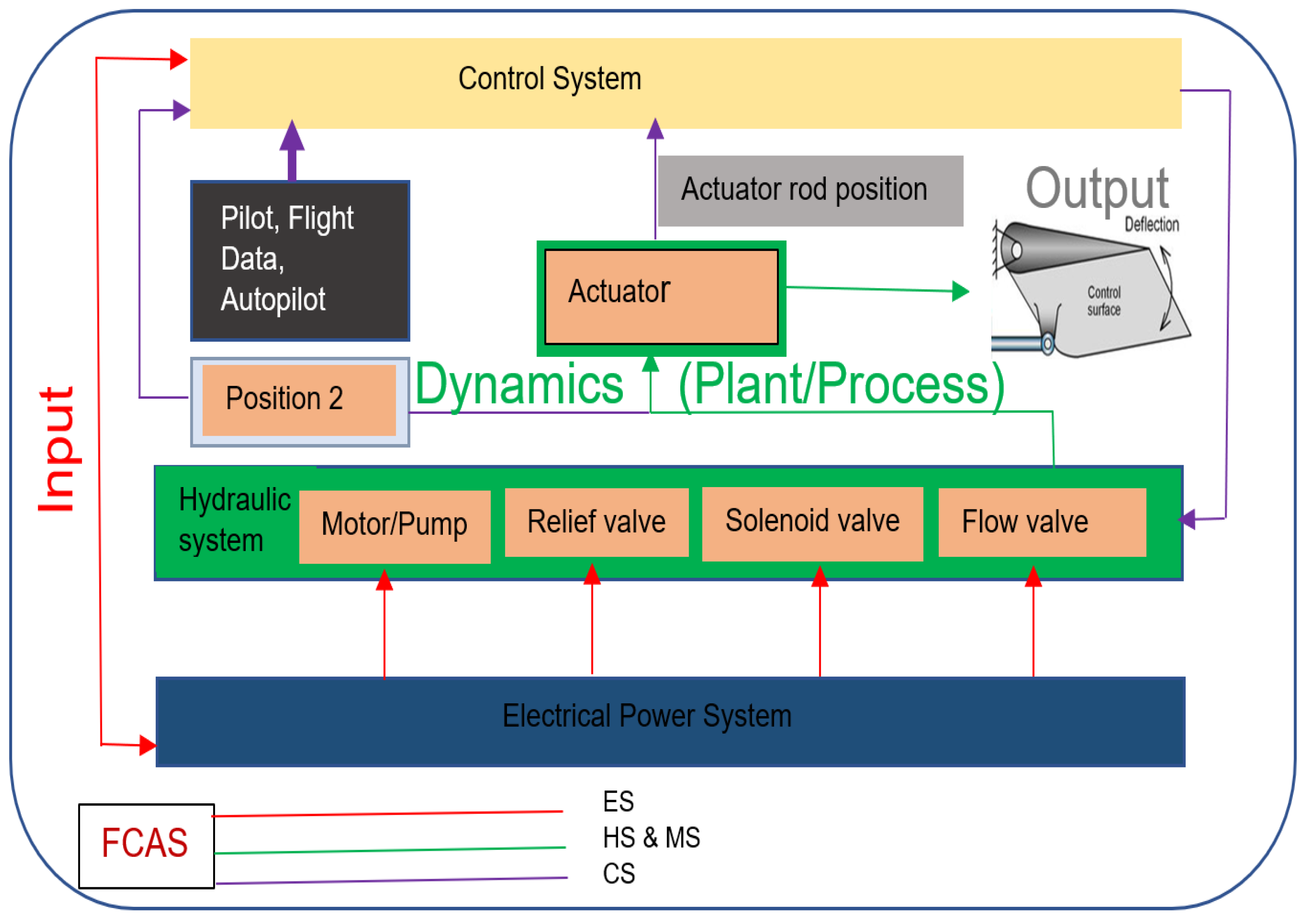
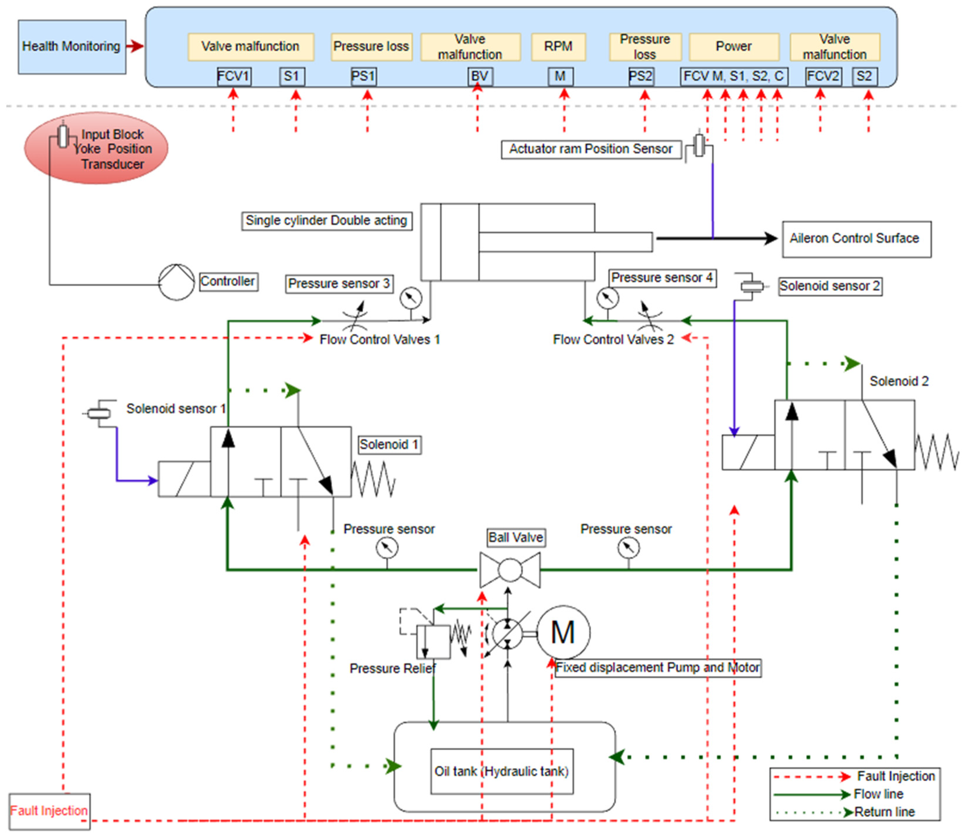
- A proposed system block diagram depicting the subsystems.
- ii.
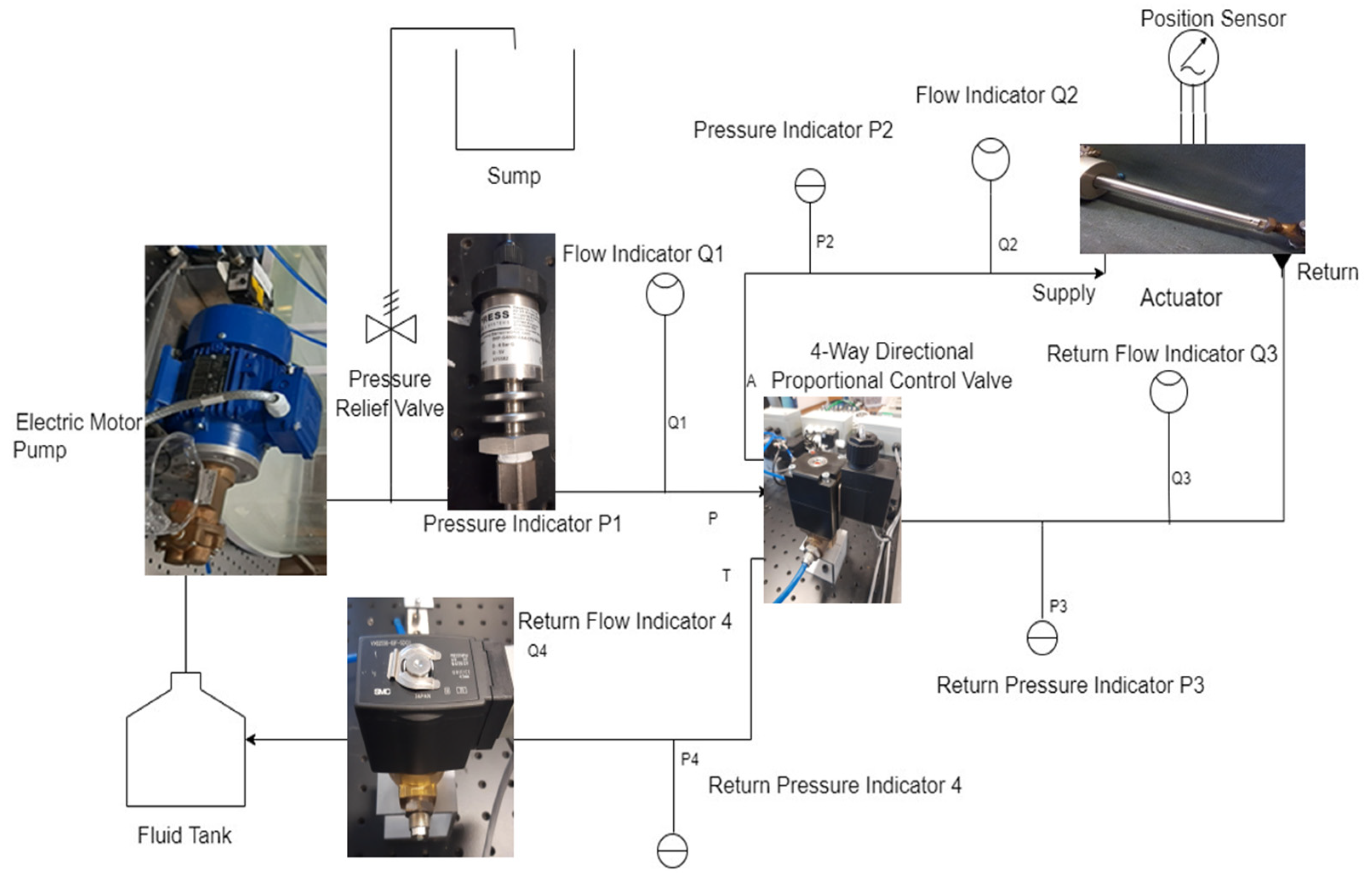
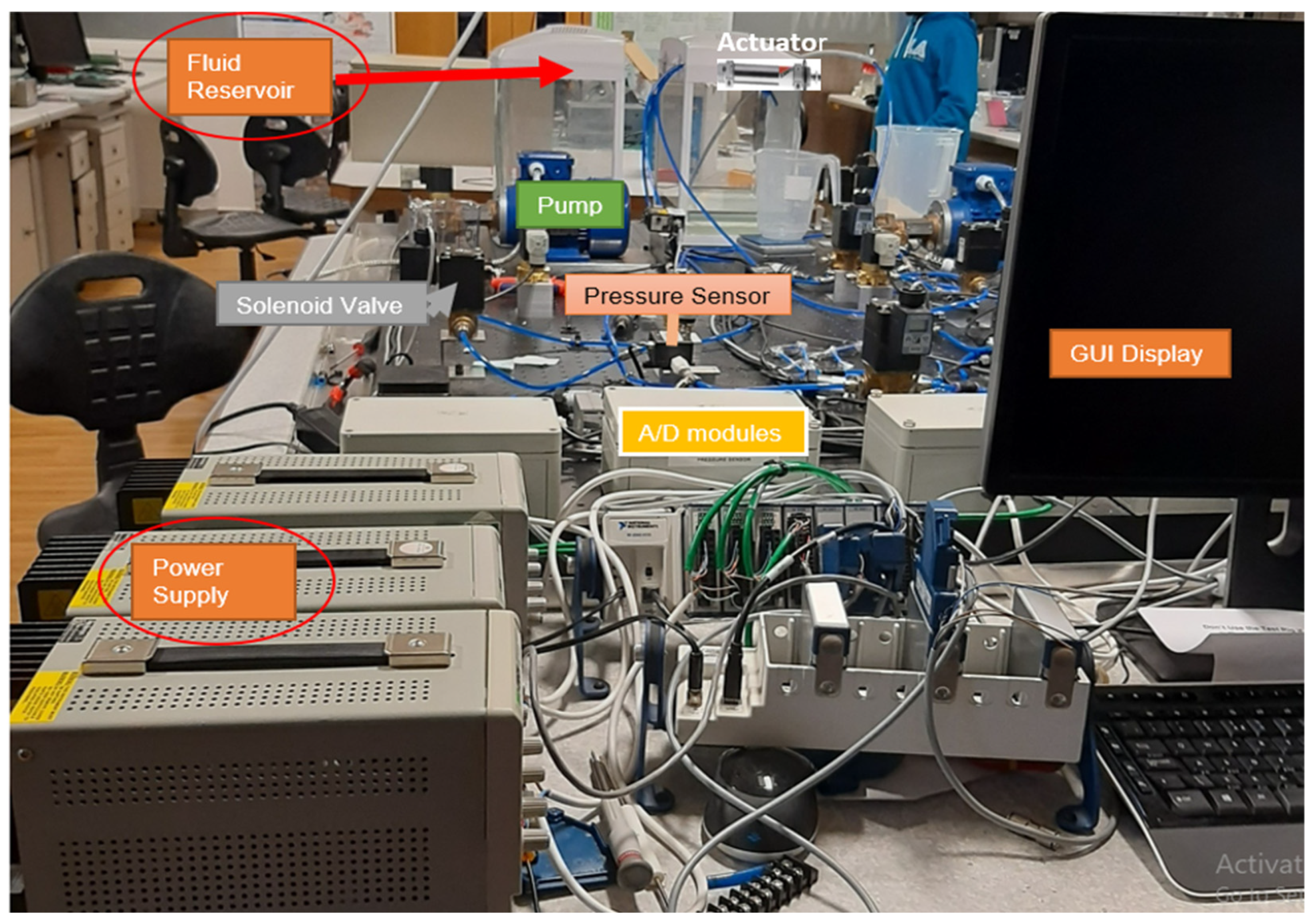
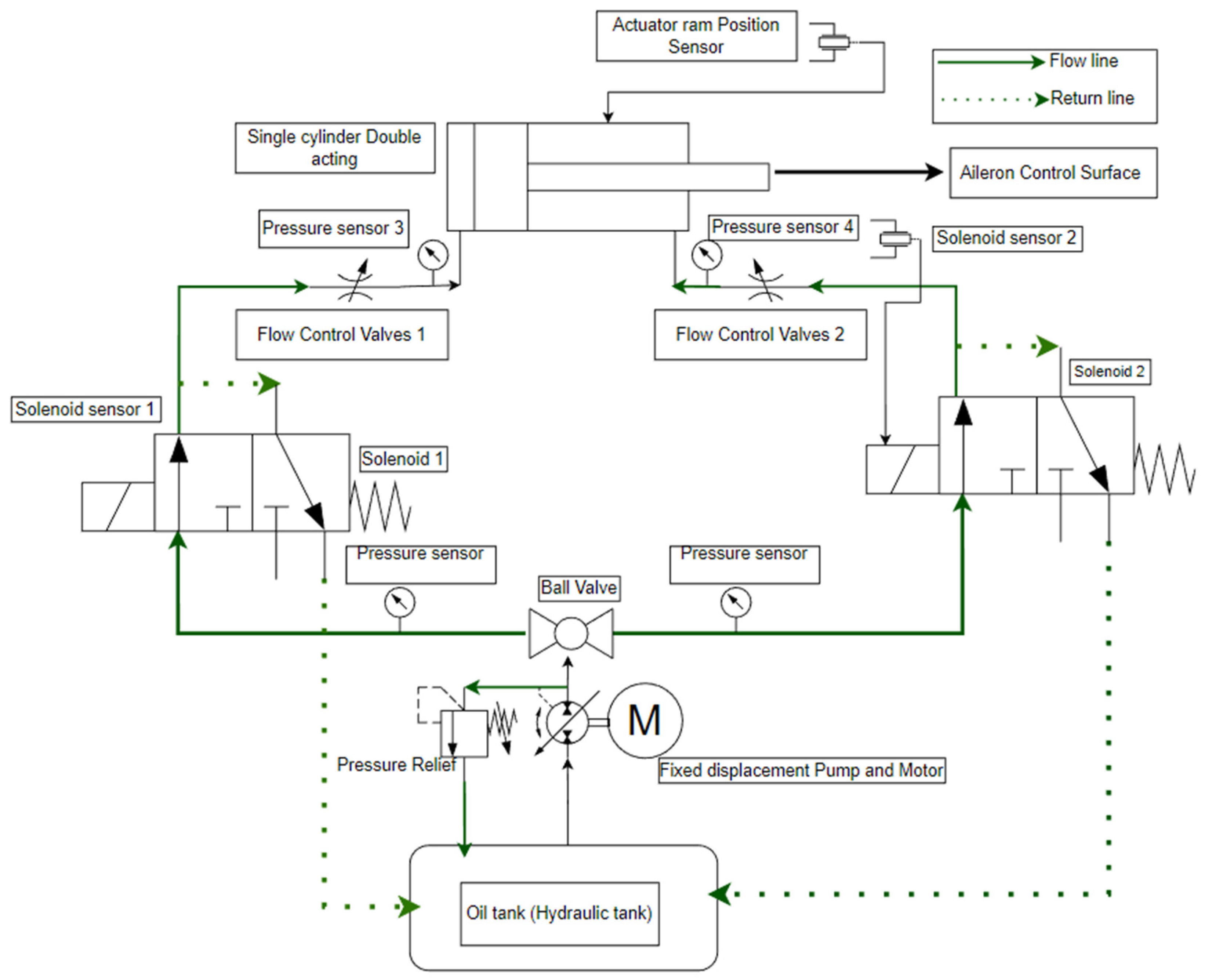
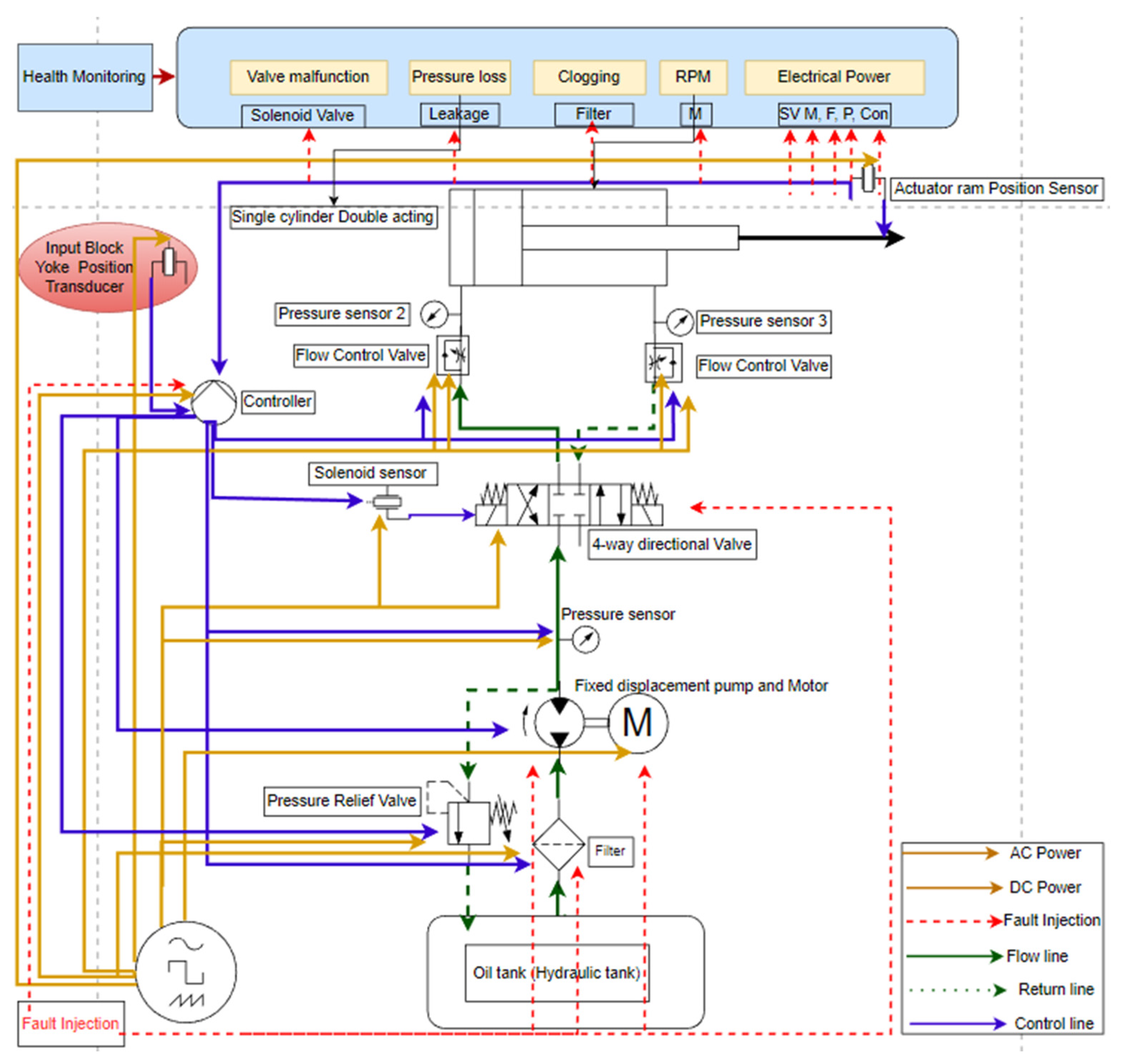
- An experimental block schematic showing how the various components were connected in the IVHM Laboratory.
- iii.
- The identified fault modes, causes, and effects.
- iv.
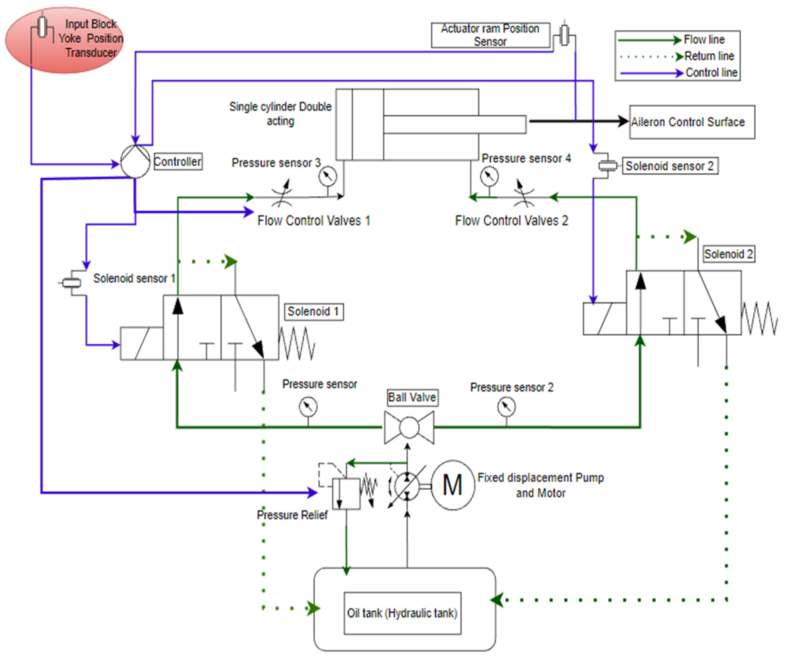
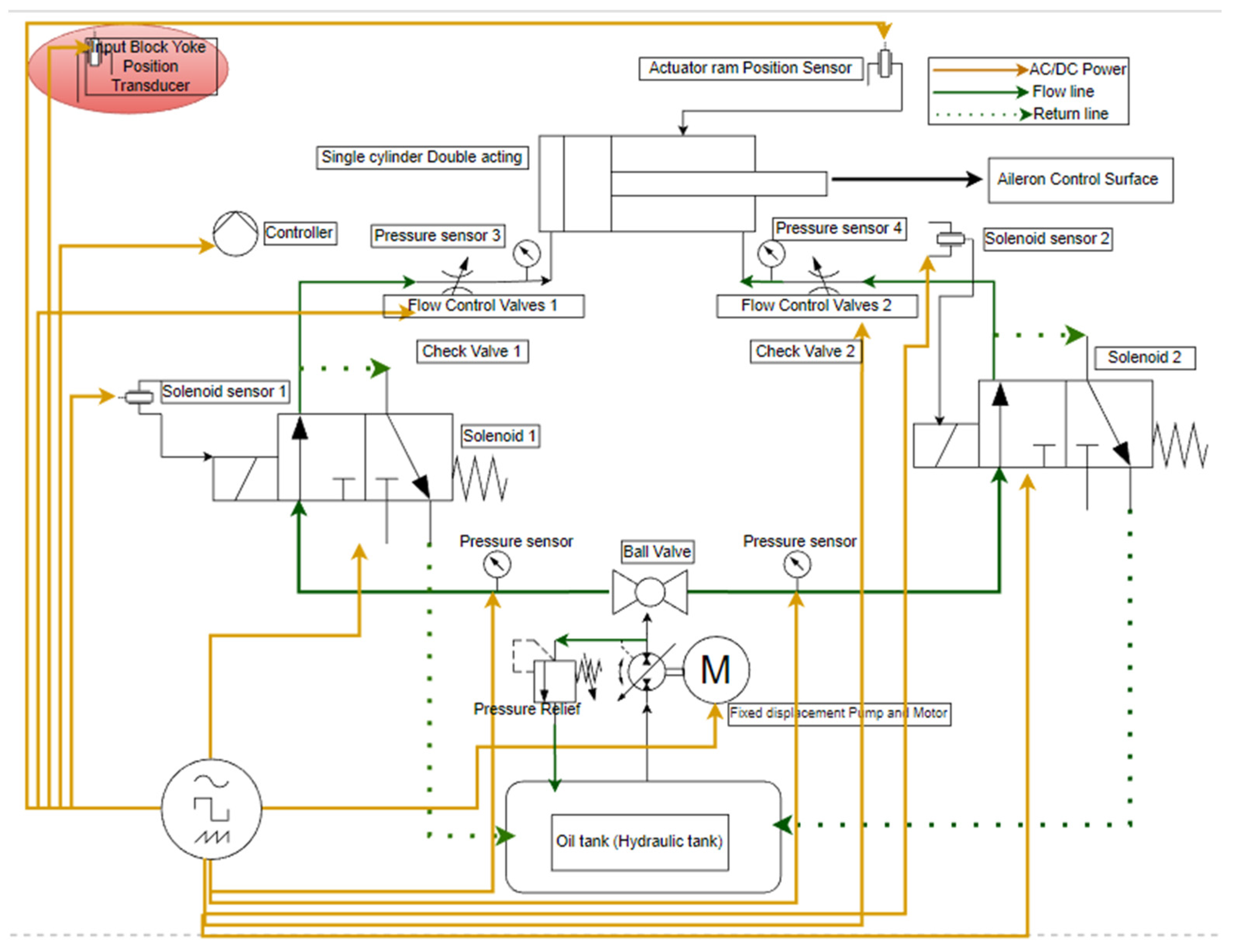
- The formation of the functional model elements and fault injection schematic.
- v.
- Simulations
3.1. Methodology and System Model Blocks
3.2. FCAS Experimental Process Block Schematic
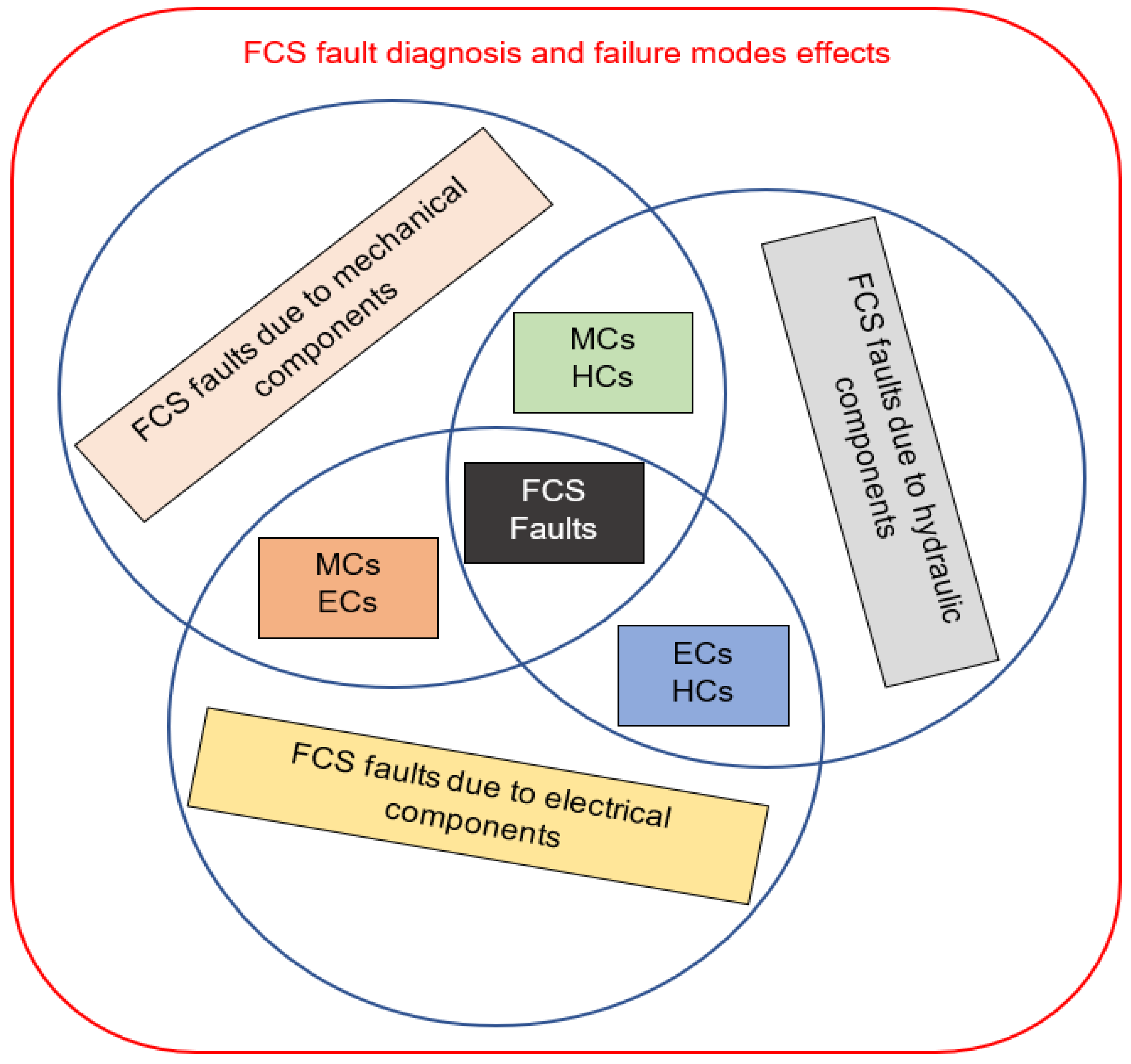
3.2.1. Identification of Fault Modes, Causes, and Effects
3.2.2. Experiment and Component Connections
3.2.3. Operating Procedure of the Preliminary Experiment
- Before the rig was operated, the operator ensured the following:
- The power supplies were switched on.
- The main tanks were filled to the required quantity of fluid by visually inspecting the tanks for their integrity and that the tanks were intact.
- Two converters, CDAQ-9172 devices, were switched on.
- The button for the motor drives situated below the emergency button was switched on.
- The PC was switched on and LabVIEW launched (this allows the Modified Fuel Rig System file in the Fuel Rig system project folder to be created):
- Experiments were run and stopped at intervals of 10s each.
- Readings were taken and saved for healthy cases.
- Then faults were injected for unhealthy scenarios, and the procedures were repeated.
4. Derivation of Boundary Conditions for Steady-State Simulation Model Parameters
Developing Subsystem Models for Fault Injection
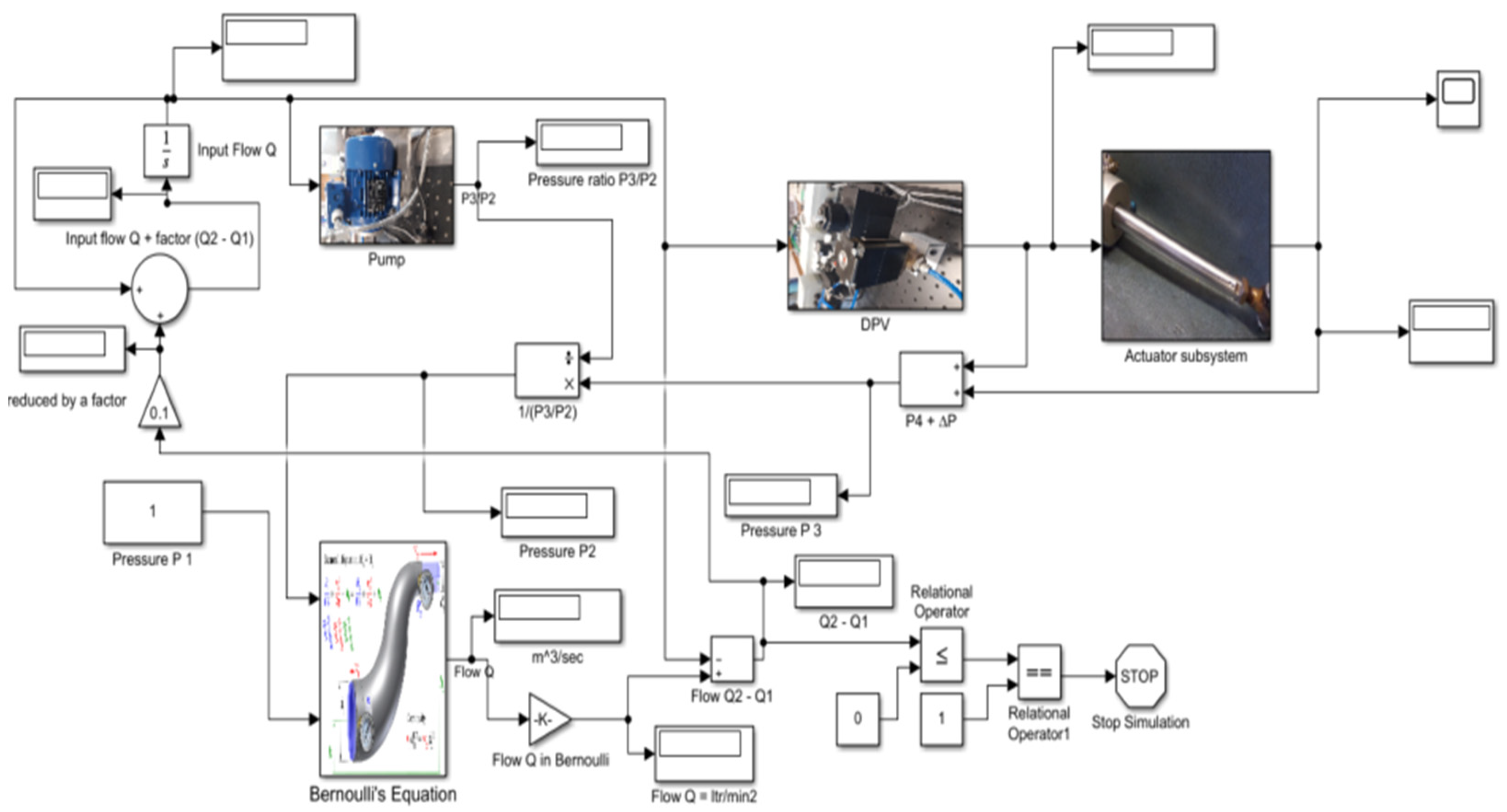
5. HPFCAS Model Development and Simulations
5.1. Simulations at Steady State
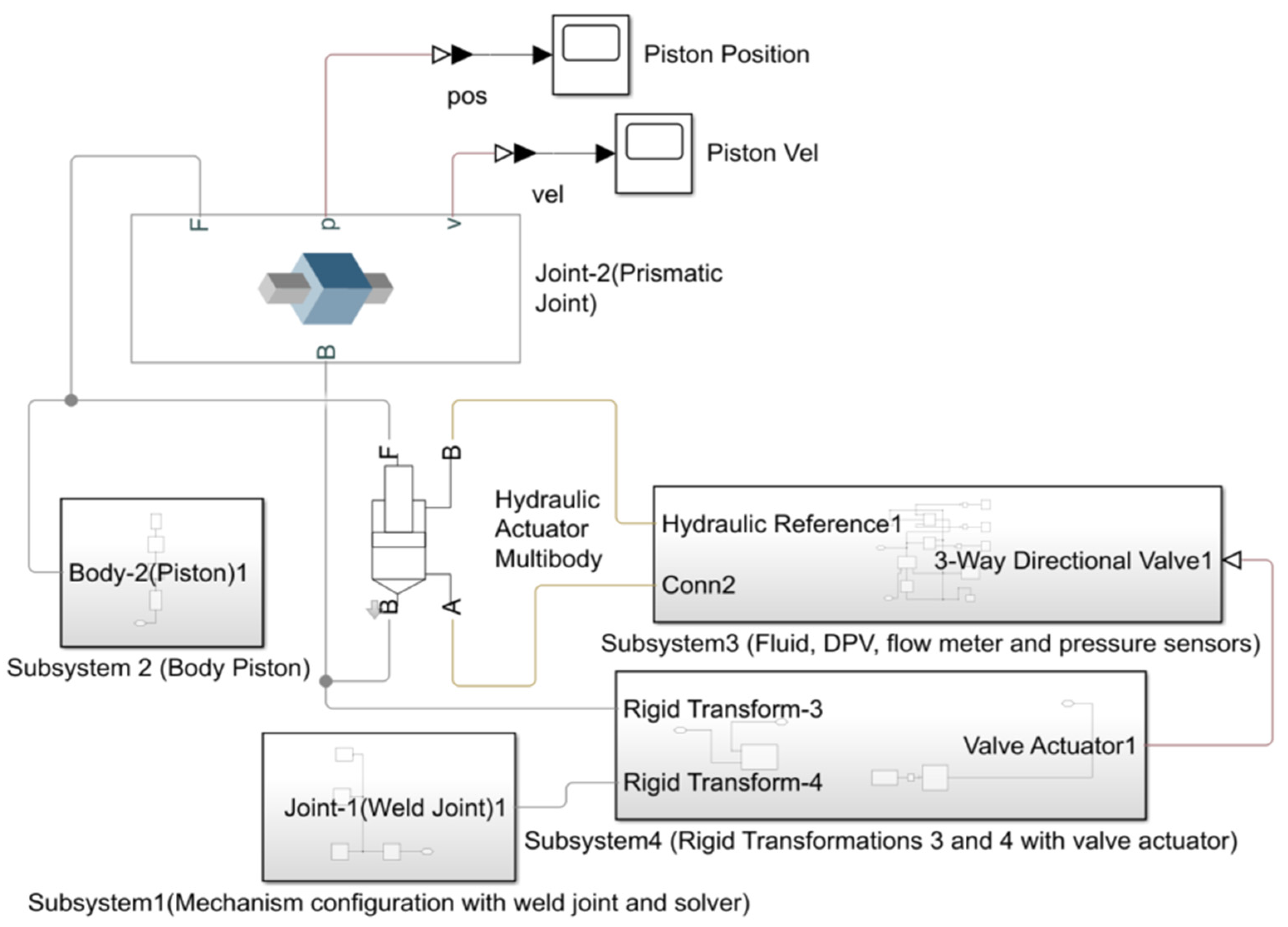
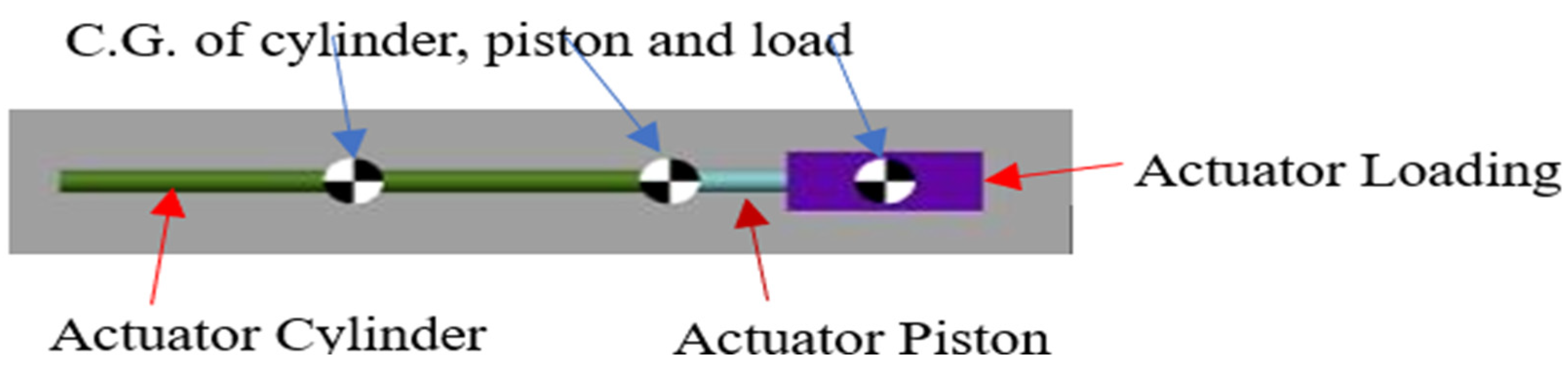
5.2. Procedures for Actuator Integration with the Model
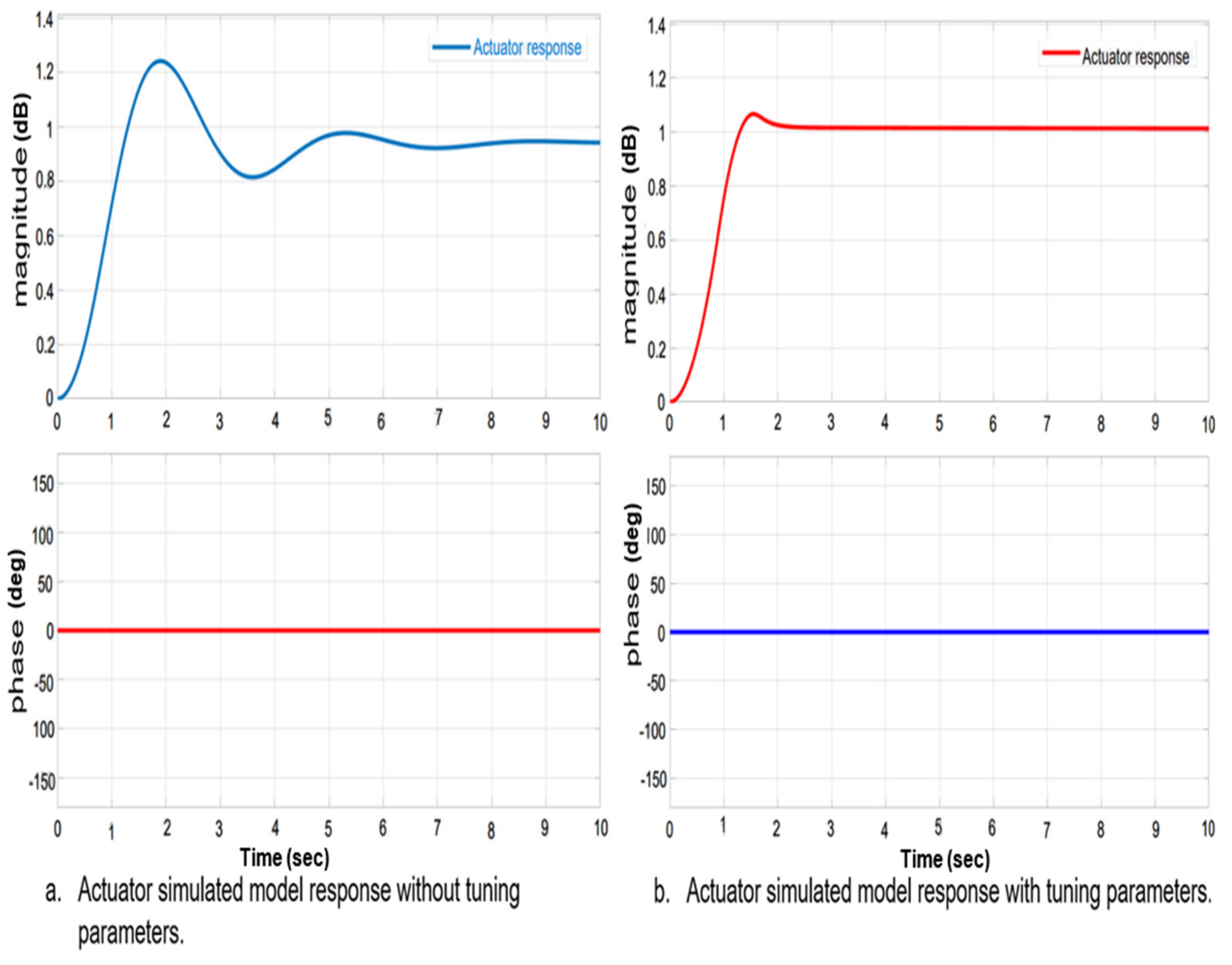
5.3. Simulations of Model in a Transient State
6. Results and Discussions
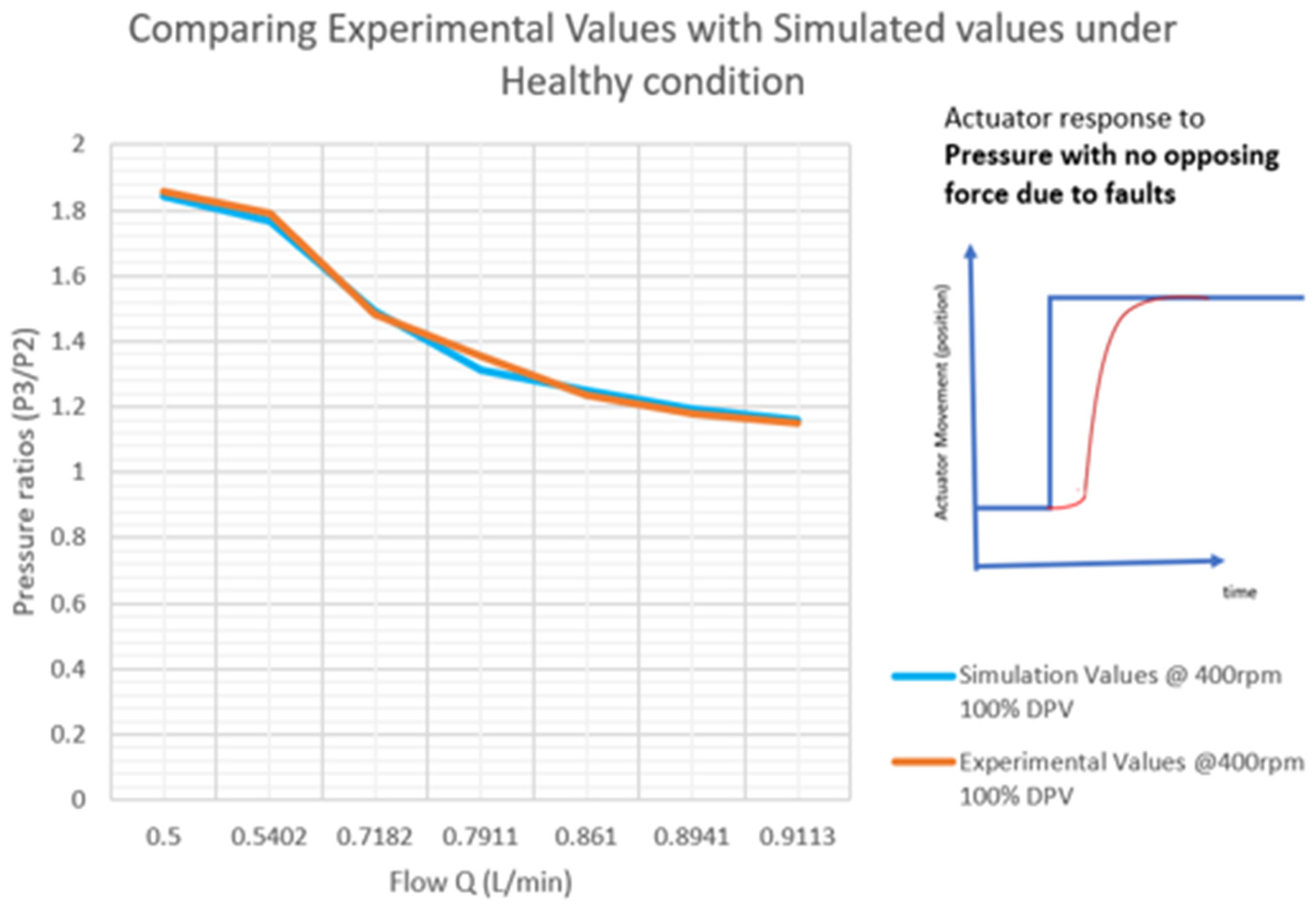
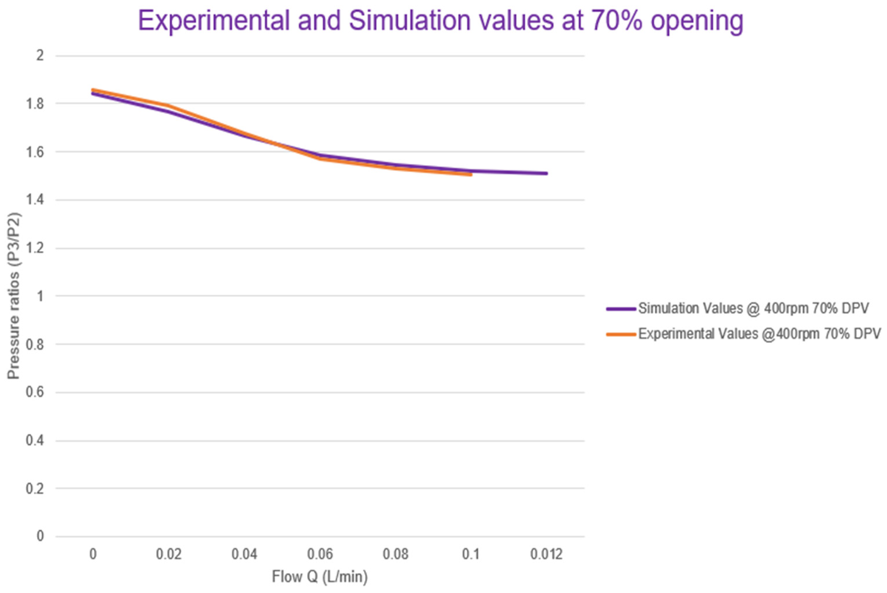
6.1. Healthy Cases
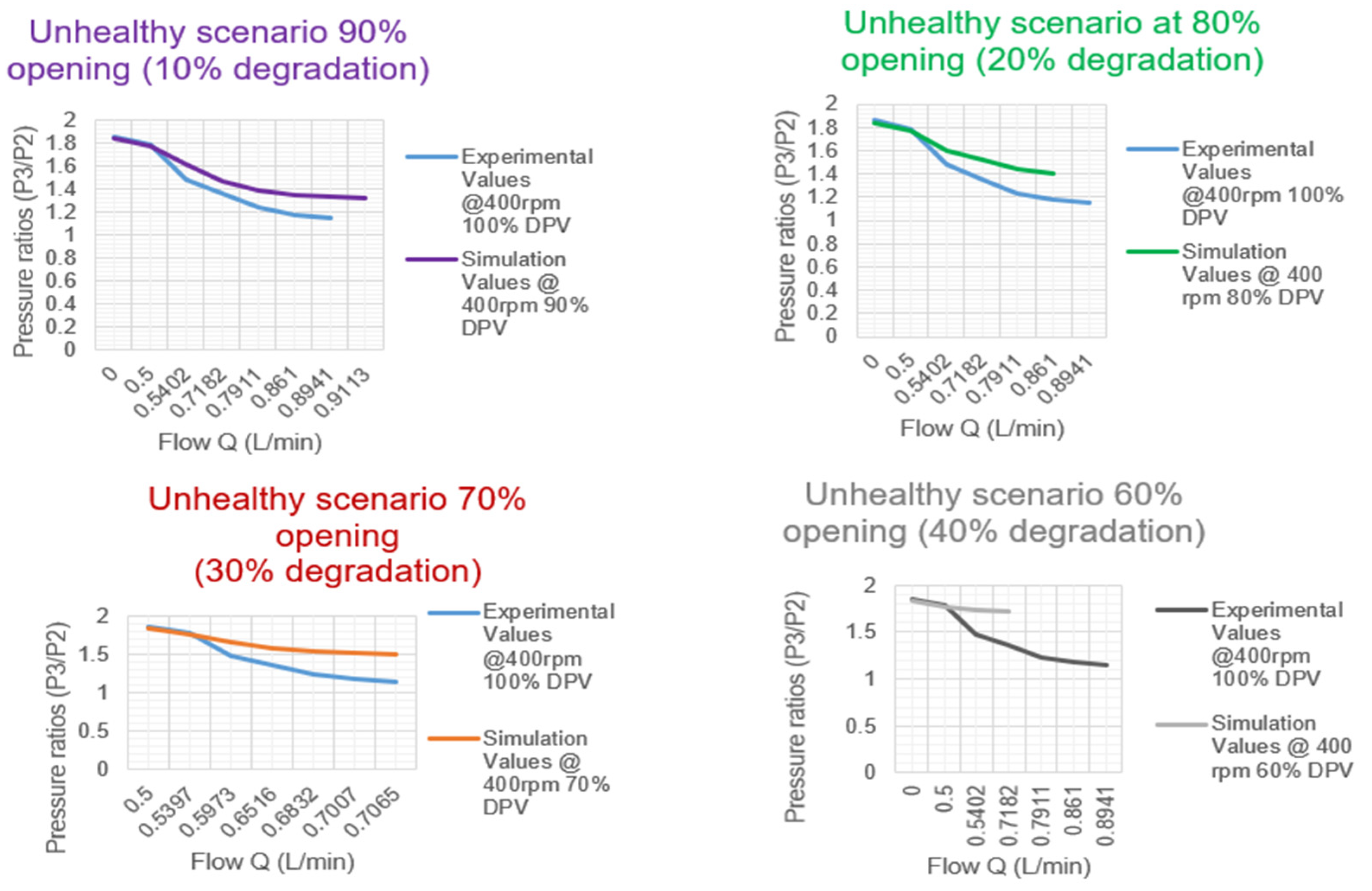
6.2. Unhealthy Cases
7. Conclusions
- In the hydraulic system, any single system or component failure, e.g., an actuator, valve, or leakage, is a principal failure mode and can trigger multiple faults.
- Any combination of failures (e.g., dual electrical and hydraulic system failures or any single failure in combination with any probable hydraulic or electrical failure) are principal faults.
- Common-mode failures/single failures (e.g., leakage) are principal failure modes that can affect multiple systems.
- In the absence of the required data, the development of suitable models for the HPFCAS for the different performance conditions generated sufficient data that were used to carry out the analysis.
- The data generated were classified and are to be used to train algorithms for diagnostics. It is proposed that this model approach can be completed appropriately for all systems.
8. Future Work and Challenges
Author Contributions
Funding
Institutional Review Board Statement
Informed Consent Statement
Data Availability Statement
Acknowledgments
Conflicts of Interest
Nomenclature
| AP | Autopilot |
| AC | Alternating Current |
| CBM | Condition Based Maintenance |
| CND | Can Not Display |
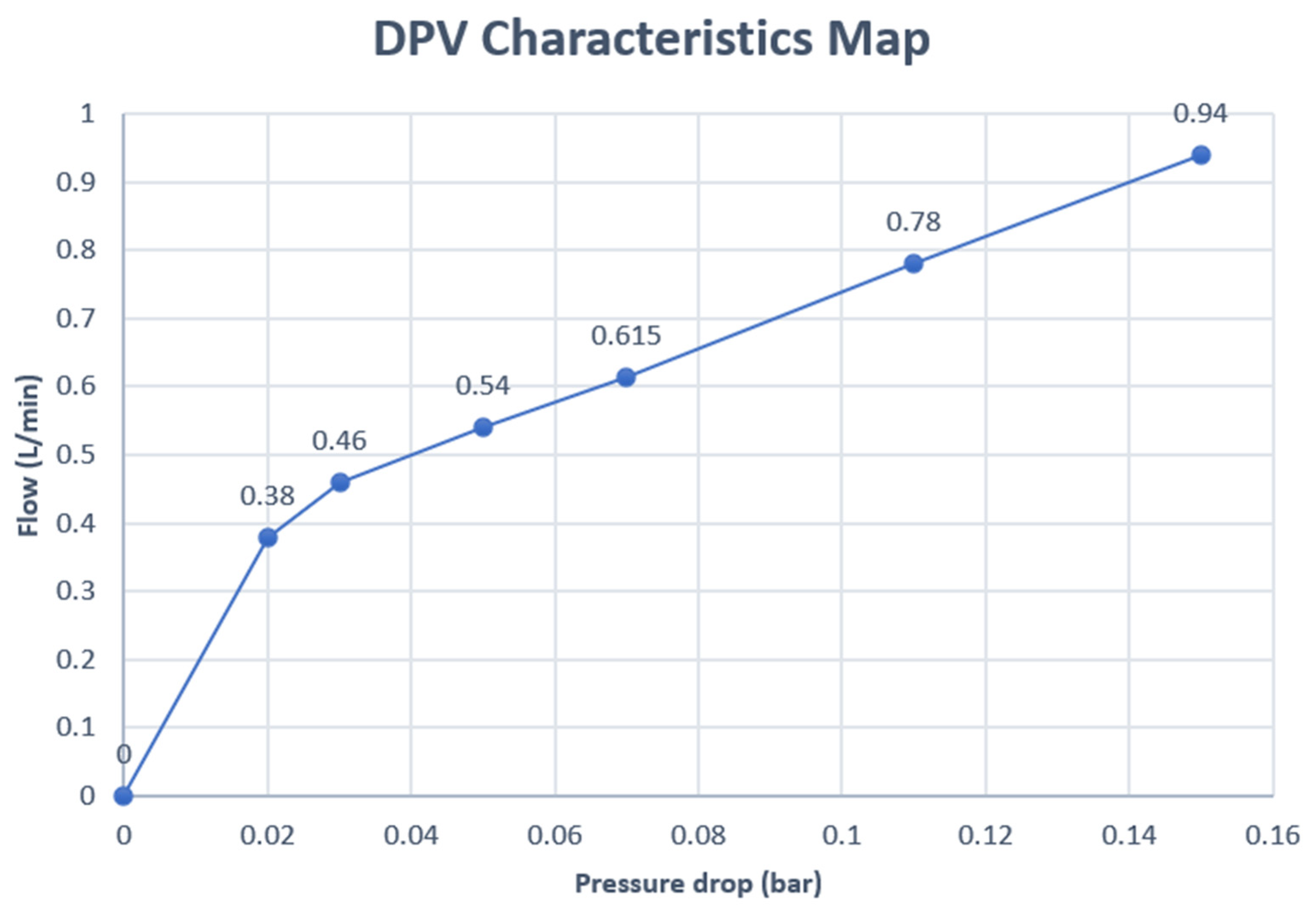
| DPV | Directional Proportional Valve |
| DC | Direct Current |
| ECs | Electrical Components |
| FC | Flight Controls |
| FCAS | Flight Control Actuation System |
| FCS | Flight Control System |
| FDI | fault Detection and Isolation |
| FF | Fault Found |
| FMECA | Failure Modes Effects and Criticality Analysis |
| FTA | Fault Tree Analysis |
| HCs | Hydraulic Components |
| HPFCAS | Hydraulically Powered Flight Control Actuator System |
| IVHM | Integrated Vehicle Health Monitoring |
| KF | Kalman Filter |
| MCs | Mechanical Components |
| MFCAS | Mechanical Flight Control Actuation System |
| NFF | No Fault Found |
| PFCAS | Primary Flight Control Actuation System |
| PHM | Prognostics Health Monitoring |
| SOS | System of systems |
| RPM | Revolution Per Minute |
| RUF | Remaining Useful Life |
| VAC | Volt Alternating Current |
| VDC | Volt Direct Current |
References
- Moir, I.; Seabridge, A. Aircraft Systems: Mechanical, Electrical and Avionics Subsystems Integration; John Wiley & Sons: Oxford, UK, 2008. [Google Scholar]
- Du, J.; Wang, S.; Zhang, H. Layered clustering multi-fault diagnosis for hydraulic piston pump. Mech. Syst. Signal Process 2013, 36, 487–504. [Google Scholar] [CrossRef]
- Peter, D. Hydraulic Control Systems Design and Analysis of Their Dynamics. In Hydraulic Control Systems Design and Analysis of Their Dynamics; Dransfield, P., Ed.; Lecture Notes in Control and Information Sciences; Springer: Berlin/Heidelberg, Germany, 1981; Volume 33. [Google Scholar]
- Dai, J.; Tang, J.; Huang, S.; Wang, Y. Signal-Based Intelligent Hydraulic Fault Diagnosis Methods: Review and Prospects. Chin. J. Mech. Eng. 2019, 32, 75. [Google Scholar] [CrossRef]
- Jennions, I.; Ali, F.; Miguez, M.E.; Escobar, I.C. Simulation of an aircraft environmental control system. Appl. Therm. Eng. 2020, 172, 114925. [Google Scholar] [CrossRef]
- Moher, D.; Liberati, A.; Tetzlaff, J.; Altman, D.G.; The PRISMA Group. Preferred reporting items for systematic reviews and meta-analyses: The PRISMA statement. BMJ 2009, 339, b2535. [Google Scholar] [CrossRef] [PubMed]
- Ezhilarasu, C.M.; Skaf, Z.; Jennions, I.K. The application of reasoning to aerospace Integrated Vehicle Health Management (IVHM): Challenges and opportunities. Prog. Aerosp. Sci. 2019, 105, 60–73. [Google Scholar] [CrossRef]
- Halder, P. A Novel Approach for Detection and Diagnosis of Process and Sensor Faults in Electro-Hydraulic Actuator. Int. J. Eng. Res. Dev. 2013, 6, 15–22. [Google Scholar]
- Castaldi, P.; Mimmo, N.; Simani, S. Avionic Air Data Sensors Fault Detection and Isolation by means of Singular Perturbation and Geometric Approach. Sensors 2017, 17, 2202. [Google Scholar] [CrossRef] [PubMed]
- Cusati, V.; Corcione, S.; Memmolo, V. Impact of Structural Health Monitoring on Aircraft Operating Costs by Multidisciplinary Analysis. Sensors 2021, 21, 6938. [Google Scholar] [CrossRef]
- Pratt, R.W. Flight Control Systems: Practical Issues in Design and Implementation (No. 57). Available online: https://api.semanticscholar.org/CorpusID:106524734 (accessed on 25 January 2024).
- Stricker, P.A. Aircraft Hydraulic System Design, Eaton Aerospace Hydraulic System Division, Report. 2010. Available online: http://www.ieeems.org/Meetings/presentations/MS2-IEEE_Hyd_Systems_Presentation.ppt (accessed on 12 January 2023).
- Skliros, C.; Ali, F.; Jennions, I. Fault simulations and diagnostics for a Boeing 747 Auxiliary Power Unit. Expert Syst. Appl. 2021, 184, 115504. [Google Scholar] [CrossRef]
- Schroeder, G.; Steinmetz, C.; Pereira, C.; Espindola, D. Digital twin data modelling with automation and a communication methodology for data exchange. IFAC-PapersOnLine 2016, 49, 12–17. [Google Scholar] [CrossRef]
- Ezhilarasu, C.M.; Jennions, I.K. Development and Implementation of a Framework for Aerospace Vehicle Reasoning (FAVER). IEEE Access 2021, 9, 108028–108048. [Google Scholar] [CrossRef]
- Skliros, C.; Miguez, M.E.; Fakhre, A.; Jennions, I. A review of model based and data driven methods targeting hardware systems diagnostics. Diagnostyka 2018, 20, 3–21. [Google Scholar] [CrossRef]
- M´arton, L.; Ossmann, D. Energetic Approach for Control Surface Disconnection Fault Detection in Hydraulic Aircraft Actuators. In Proceedings of the 8th IFAC Symposium on Fault Detection, Supervision and Safety of Technical Processes (SAFEPROCESS), Mexico City, Mexico, 29–31 August 2012. [Google Scholar]
- An, L.; Sepehri, N. Hydraulic actuator leakage fault detection using extended Kalman filter. Int. J. Fluid Power 2005, 6, 41–51. [Google Scholar] [CrossRef]
- Ritto, T.; Rochinha, F. Digital twin, physics-based model, and machine learning applied to damage detection in structures. Mech. Syst. Signal Process 2021, 155, 107614. [Google Scholar] [CrossRef]
- Byington, C.S.; Matthew, P.E.; Edwards WDStoelting, P. A Model-Based Approach to Prognostics and Health Management for Flight Control Actuators. In Proceedings of the IEEE Aerospace Conference, Big Sky, MT, USA, 6–13 March 2004. [Google Scholar]
- Iyaghigba, S.D.; Ali, F.; Jennions, I.K. A Review of Diagnostic Methods for Hydraulically Powered Flight Control Actuation Systems. Machines 2023, 11, 165. [Google Scholar] [CrossRef]
- Ismail, M.A.A.; Balaban, E.; Windelberg, J. Spall Fault Quantification Method for Flight Control Electromechanical Actuator. Actuators 2022, 11, 29. [Google Scholar] [CrossRef]
- Moir, I.; Seabridge, A. Civil Avionics Systems, 2nd ed.; John Wiley & Son, Ltd.: Hoboken, NJ, USA, 2013; Available online: https://onlinelibrary.wiley.co (accessed on 25 January 2024).
- Lin, Y. System Diagnosis Using a Bayesian Method. Ph.D. Thesis, Cranfield University, Cranfield, UK, 2017. [Google Scholar]
- Ezhilarasu, C.M.; Skaf, Z.; Jennions, I.K. A Generalised Methodology for the Diagnosis of Aircraft Systems. IEEE Access 2021, 9, 11437–11454. [Google Scholar] [CrossRef]
- Vachtsevanos, G.; Lewis, F.L.; Roemer, M.; Hess, A.; Wu, B. Intelligent Fault Diagnosis and Prognosis for Engineering System; John Wiley & Sons, Inc.: Hoboken, NJ, USA, 2006. [Google Scholar]
- Zhao, Z.; Wang, F.L.; Jia, M.X.; Wang, S. Intermittent-chaos-and-cestrum-analysis-based early fault detection on shuttle valve of hydraulic tube tester. IEEE Trans. Ind. Electron. 2009, 56, 2764–2770. [Google Scholar] [CrossRef]
- Huang, J.; An, H.; Lang, L.; Wei, Q.; Ma, H. A Data-Driven Multi-Scale Online Joint Estimation of States and Parameters for Electro-Hydraulic Actuator in Legged Robot. IEEE Access 2020, 8, 36885–36902. [Google Scholar] [CrossRef]
- Waszecki, P.; Kauer, M.; Lukasiewycz, M.; Chakraborty, S. Implicit Intermittent Fault Detection in Distributed Systems. In Proceedings of the 19th Asia and South pacific Design Automation Conference (ASP-DAC) TUM CREATE, Singapore, 23 January 2014. [Google Scholar] [CrossRef]
- Ferrell, B.L. JSF Prognostics and Health Management. In Proceedings of the IEEE Aerospace Conference, Big Sky, MO, USA, 6–13 March 1999. [Google Scholar] [CrossRef]
- Nesbitt, B. Properties of fluids. In A Handbook of Valves and Actuators; Butterworth-Heinemann: Oxford, UK, 2007; pp. 43–79. [Google Scholar] [CrossRef]
- Ding, Q.; Peng, X.; Zhong, X.; Hu, X. Fault Diagnosis of Nonlinear Uncertain Systems with Triangular Form. J. Control. Sci. Eng. 2017, 2017, 6354208. [Google Scholar] [CrossRef]
- Huang, K.; Wu, S.; Li, F.; Yang, C.; Gui, W. Fault Diagnosis of Hydraulic Systems Based on Deep Learning Model with Multirate Data Samples. IEEE Trans. Neural Netw. Learn. Syst. 2022, 33, 6789–6801. [Google Scholar] [CrossRef]
- Esperon-Miguez, M.; John, P.; Jennions, I.K. A review of Integrated Vehicle Health Management tools for legacy platforms: Challenges and opportunities. Prog. Aerosp. Sci. 2012, 56, 19–34. [Google Scholar] [CrossRef]
- Linaric, D.; Koroman, V. Fault Diagnosis of a Hydraulic Actuator using Neural Network. In Proceedings of the IEEE International Conference on Industrial Technology (CIT 2003): 4th International Conference on Industrial Tools, Maribor, Slovenia, 10–12 December 2003; pp. 108–111. [Google Scholar]
- Janizadeh Haji, B.; Bamdad, M. Steady-state dynamic analysis of a nonlinear fluidic soft actuator. J. Vib. Control 2023, 29, 1606–1625. [Google Scholar] [CrossRef]
- Hiremath, S.S.; Singaperumal, M. Investigations on Actuator Dynamics through Theoretical and Finite Element Approach. Math. Probl. Eng. 2010, 2010, 191898. [Google Scholar] [CrossRef]
- Van der Auweraer, H. Connecting Physics Based and Data Driven Models: The Best of Two Worlds. 2018. Available online: https://www.ima.umn.edu/materials/2017-2018/SW3.6-8.18/26842/IMA_2018_Van_der_Auweraer.pdf (accessed on 3 April 2019).
- Zhou, Y.; Su, Y.; Xu, Z.; Wang, X.; Wu, J.; Guan, X. A hybrid physics-based/data-driven model for personalized dynamic thermal comfort in ordinary office environment. Energy Build. 2021, 238, 110790. [Google Scholar] [CrossRef]
- Mazzoleni, M.; Maccarana, Y.; Previdi, F. A comparison of data-driven fault detection methods with application to aerospace electro-mechanical actuators. IFAC-PapersOnLine 2017, 50, 12797–12802. [Google Scholar] [CrossRef]
- Xu, J.; Yoon, H.-S. A Review on Mechanical and Hydraulic System Modeling of Excavator Manipulator System. J. Constr. Eng. 2016, 2016, 9409370. [Google Scholar] [CrossRef]
- Peng, X.; Xu, H.; Wang, J.; Liu, J.; He, C. Ensemble Multiple Distinct ResNet Networks With Channel-Attention Mechanism for Multisensor Fault Diagnosis of Hydraulic Systems. IEEE Sens. J. 2023, 23, 10706–10717. [Google Scholar] [CrossRef]


| Failure Modes | Causes of Faults | Effects | Failure Types |
|---|---|---|---|
| HPFCAS1 | Filter Clogging | Decrease in pressure | Mechanical, Hydraulic |
| HPFCAS2 | Pipe Leaking | Decrease in pressure | Mechanical, Hydraulic |
| HPFCAS3 | Motor (demagnetization) loss of output to the pump | Decrease in rpm | Mechanical, Electrical |
| HPFCAS4 | Low power to the electric pump | Decrease in rpm or no pressure | Electrical |
| HPFCAS5 | Clogged nozzle/malfunction (flow control valve NRV) | Decrease or no pressure, damage to the flow line | Mechanical, Hydraulic |
| HPFCAS6 | Low power to the flow control valve (Solenoid valve) | No pressure, damage to the flow lines | Electrical, Hydraulic |
| HPFCAS7 | Temperature rise (windings, heat) | More power required, pressure decrease | Thermal, Mechanical, Electrical |
| HPFCAS8 | Vibrations (electrical connections, position sensor measurements) | Actuator components, electrical cables, | Electrical, sensors |
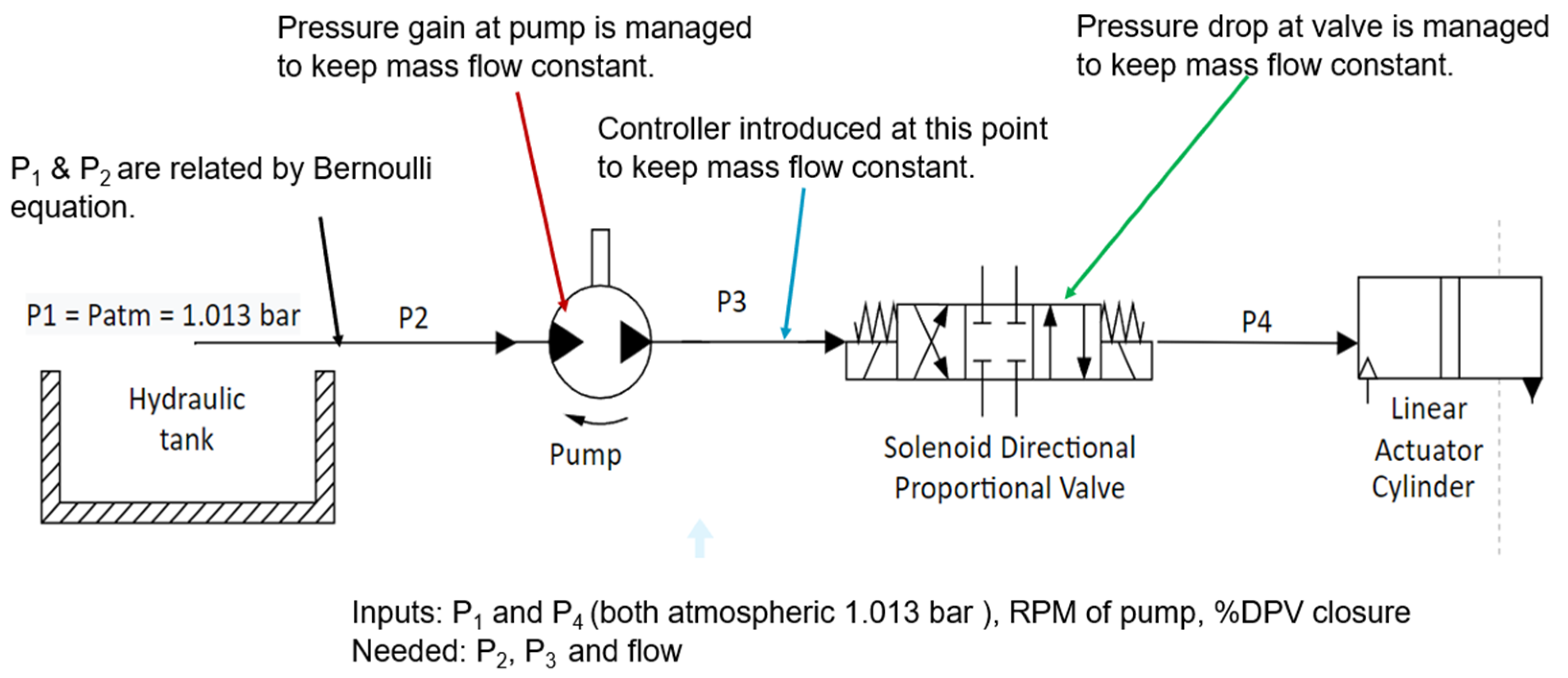
| Inputs | Initial Boundary Conditions | Descriptions |
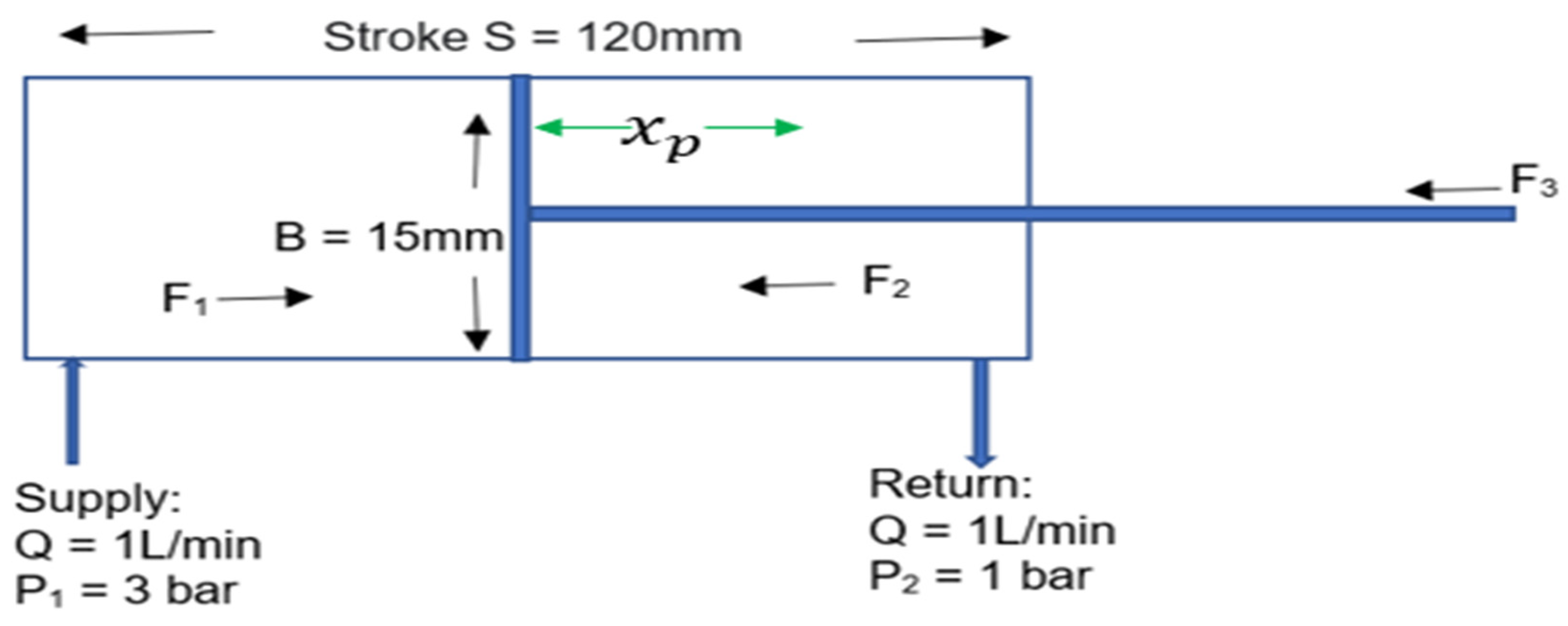
| i (Pressure values) | P1 and P4 | both atmospheric |
| ii (Rpm settings) | 400 | RPM of pump |
| iii (DPV opening) | 100% | RPM of pump |
| Iv (Pressure values) | P2 and P3 | Unknowns |
| Process | ||
| i (Flow rate values) | 0.5 L/min | Guess mass flow |
| ii (Pressure values) | P3 | Obtained from DPV curve |
| iii (Pressure ratio values) | P3/P2 | Obtained from pump curve |
| iv (Flow rate values) | Flow | Obtained from Bernoulli using stations 1 and 2 |
| v (Flow rate values) | Mass flow | Adjust the flow rate and repeat the process. |
Disclaimer/Publisher’s Note: The statements, opinions and data contained in all publications are solely those of the individual author(s) and contributor(s) and not of MDPI and/or the editor(s). MDPI and/or the editor(s) disclaim responsibility for any injury to people or property resulting from any ideas, methods, instructions or products referred to in the content. |
© 2024 by the authors. Licensee MDPI, Basel, Switzerland. This article is an open access article distributed under the terms and conditions of the Creative Commons Attribution (CC BY) license (https://creativecommons.org/licenses/by/4.0/).
Share and Cite
Iyaghigba, S.D.; Petrunin, I.; Avdelidis, N.P. Modeling a Hydraulically Powered Flight Control Actuation System. Appl. Sci. 2024, 14, 1206. https://doi.org/10.3390/app14031206
Iyaghigba SD, Petrunin I, Avdelidis NP. Modeling a Hydraulically Powered Flight Control Actuation System. Applied Sciences. 2024; 14(3):1206. https://doi.org/10.3390/app14031206
Chicago/Turabian StyleIyaghigba, Samuel David, Ivan Petrunin, and Nicolas P. Avdelidis. 2024. "Modeling a Hydraulically Powered Flight Control Actuation System" Applied Sciences 14, no. 3: 1206. https://doi.org/10.3390/app14031206