A Clutter Identification and Removal Method Based on Long Delay Lines and Cross-Correlation in Through-Wall Detection

Abstract

Life detection is important in earthquake rescue, but weak vital signal is susceptible to interference by clutters. Due to the undesirable characteristics of the hardware, there are two main types of clutter generated by the frequency modulation continuous wave (FMCW) radar when transmitting signals. One is generated by periodic nonlinearity during frequency modulation, and the other is generated by the phase-locked loop spuriousness (PLLS) in frequency division. They cause additional beat frequencies to appear beside those from the target, leading to false alarms. Since the suppression measures for them are different, it is necessary to distinguish the types of clutter and choose appropriate suppression methods. In this paper, the accurate theoretical modeling of the effects of the periodic nonlinearity and phase-locked loop spuriousness on the beat signal is performed to determine distinctions between them. The clutter occurring in the system used is identified as originating from phase-locked loop spuriousness through fiber-optic experiments. A method using long delay lines and cross-correlation is proposed to identify and remove it. In experiments, the false alarm rate is reduced from over 50 percent to nearly 0 percent, providing strong evidence for the effectiveness of the proposed method in through-wall detection.

1. Introduction

In recent years, non-contact respiration detection as the vital sign of human beings by utilizing radar systems has been widely used in medical, security, disaster rescues, and so on [1,2,3,4]. Electromagnetic waves are reflected by the human target and picked up by the radar system. The small displacement in the chest or abdominal wall associated with respiratory activity causes certain characteristics of the echo signal, such as amplitude and phase, to vary with time. This feature is not present in the echoes of other stationary subjects, and thus human targets can be recognized. Due to the penetrating nature of electromagnetic waves, through-wall detection has been widely used in concealed target detection behind obstacles [5,6]. The elaboration of the concept of small-displacement detection related to human vital signs based on a radar system and the concept of through-wall detection prompted studies to develop methods for detecting living human targets behind walls.

The frequency modulation continuous wave (FMCW) radar has been widely used in human vital sign detection due to its straightforward structure, high sensitivity, and impressive range resolution [7,8]. The breathing pattern can be detected from the phase change of the beat signal [9]. The target distance from the radar can be converted from the frequency of the beat signal. In through-wall detection, the presence of the wall causes a large attenuation of electromagnetic waves. Therefore, for the same detection range, the radar needs to have a higher power than when applied in free space. At this point, the radar with a wideband short pulse requires higher peak power, which is difficult to implement in hardware. However, this is not the case with the FMCW radar because of its large time-width bandwidth product. Moreover, the FMCW radars have a higher degree of device integration, which makes it easy to achieve miniaturization. These make the FMCW radar more suitable for through-wall detection. However, FMCW radar suffers from two types of clutter during transmission due to the undesirable characteristics of the hardware. One is generated by the nonlinear frequency modulation, and the other is generated by the phase-locked loop spuriousness that arises in system frequency division. They cause additional beat frequencies to appear beside those from the target, leading to false alarms.

More seriously, they are further complicated by reflections from the wall, the human target, and other objects in through-wall detection [10]. These problems seriously impact the correctness of human target localization [11]. It is necessary to study the solution of removing them before performing target detection.

There are different suppression methods for these two types of clutter. For frequency modulation nonlinearities, current research includes both hardware and software correction methods. Hardware techniques include using predistortion technique to compensate for nonlinearity in voltage-controlled oscillator (VCO) response characteristics [12], correcting varactor tuning curves by a tuning voltage converter [13], using direct digital synthesizers (DDSs) [14] and phased-locked loops (PLL) [15]. However, they not only raise the cost but also increase the complexity of the system. Software corrections are divided into two steps: nonlinearity estimation and correction. Using a fixed-range target echo as reference, the estimation methods consist of coherent integration [16], homomorphic deconvolution [17], and high-order ambiguity function [18]. This effect is partially compensated using methods such as residual video phase (RVP) removal [16,19], time resampling [17,18], and match Fourier transform [20].

For the phased-locked loop spuriousness, current research focuses on hardware suppression methods. They include the use of adaptive filtering techniques [21] and a charge pump phase-locked loop architecture with dual loops [22] to suppress spuriousness to a low level. Techniques for suppressing phase-locked loop spuriousness using software methods are not yet available.

Since there are different methods for dealing with the above two types of clutter, it is necessary to check the type of clutter in the system used before selecting the method. Therefore, the difference between their effects on the beat signal has become the focus of the study. In this paper, without using any approximation, the exact effect of periodic nonlinearity and the phase-locked loop spuriousness on the beat signal is established, respectively. Their characteristics can be clearly recognized in theory. To exclude environmental effects, a series of closed-loop experiments were conducted using different lengths of optical fibers. Comparing the experimental phenomena with the above theory, the clutter that appeared in the system used is confirmed to be generated by phase-lock loop spuriousness. A removal method based on long delay lines and cross-correlation is proposed which can not only identify the location of the clutter, but also remove it. After using the proposed method, the false alarms are eliminated. The effectiveness of the proposed method is verified by experiments, including the free space and through-wall situations.

The rest of the article is organized as follows. In Section 2, theories of effects of periodic nonlinearity and phase-locked loop spuriousness on the spectrum of the beat signal are successively established. Section 3 introduces the fiber optic experiments used to identify the source of the clutter in the system. Section 4 presents the proposed method for removing the clutter. In Section 5, experimental results in free space and through-wall situations are shown to demonstrate the effectiveness of the proposed method. Finally, the conclusion is presented in Section 6.

2. Theory

2.1. Impact of Periodic Nonlinearity on the FMCW Radar

The transmitted signal of an ideal FMCW Radar system [17] can be expressed as

$$s_{t0}(t)=rect(\frac{t}{T_p})\exp [j2\pi (f_{c}t+0.5K{t}^2)],$$

(1)

where $T_p$ denotes the single frequency modulation cycle, $f_c$ denotes the center frequency, $K$ denotes the frequency sweep rate. To obtain frequency, the derivative operation on the phase of the transmitted signal is performed. The result can be expressed as $f_c+Kt$. The variation of $t$ ranges from 0 to $T_P$, so frequency $f$ varies from 0 to $f_c+K{T}_p$, which completes the frequency sweep. Thus, square term $0.5 K{t}^2$ in the phase drives the frequency sweep. Because the bandwidth of the transmitted signal is $B=K\times T_p$, the start and end frequencies are $f_l=f_c$, $f_h=f_c+B$, respectively.

The illustration of the radar wave propagation in free space is shown in Figure 1. The wave is reflected from the target with a time delay of $\tau$. The rectangular envelope limits the time range of the transmitted signal but does not affect the phase of it. Therefore, the rectangular envelope is generally ignored for the sake of simplicity in formulas. Ignoring the rectangular envelope, the ideal reflected wave can be represented as

$$s_{r0}(t)=\exp [j2\pi (f_c(t-\tau )+0.5K{(t-\tau )}^2)].$$

(2)

The reflected signal is mixed with the transmitted signal and then filtered by a low-pass filter (LPF) to obtain the ideal beat signal,

$$\begin{array}{cc}{s}_{IF0}(t)& =LPF\{s_{t0}(t)\times s_{r0}(t)\}\\ & =LPF\{\exp [j2\pi (f_c\tau +K\tau t-0.5K{\tau }^2)]\\ & \hspace{1em}\hspace{1em} +\exp \{j2\pi [(2f_c-K\tau )t+K{t}^2-f\tau +0.5K{\tau }^2]\}\}\\ & =\exp [j2\pi (f_c\tau +K\tau t-0.5K{\tau }^2)]\end{array},$$

(3)

where $LPF\{\cdot \}$ represents low-pass filtering of signals.

The schematic of the above process is shown in the first line of Figure 2. In Figure 2a, the solid and dashed lines represent the frequencies of the transmitted and received signals over time, respectively. The transformation of frequency with time is linear, i.e., linear modulation. After the above mixing and low-pass filtering, a single-frequency beat signal is obtained, as shown in Figure 2b. Fast Fourier transform (FFT) is performed on $s_{IF0}(t)$ and the result is denoted as $S_{IF0}(\omega )$. $S_{IF0}(\omega )$ is the spectrum of $s_{IF0}(t)$, which is illustrated in Figure 2c.

When the periodic nonlinearity in modulation (periodic nonlinear modulation) occurs, a periodic phase is added to the transmitted signal. To describe that, $\epsilon (t)$ is defined as the phase it brings which is assumed to follow a cosine-like pattern [11],

$$\epsilon (t)=b\cos (2\pi f_{e}t),$$

(4)

where $b$ denotes the amplitude of the periodic nonlinear phase, and $f_e$ denotes the frequency of the periodic nonlinear phase. Therefore, the actual transmitted signal [11] can be represented as

$$s_{t1}(t)=\exp \{j[2\pi (f_{c}t+0.5K{t}^2)+\epsilon (t)]\}.$$

(5)

After reflection from the target with time delay $\tau$, the periodic nonlinearity is carried into the received signal. The actual reflected wave is expressed as

$$s_{r1}(t)=\exp \{j[2\pi (f_c(t-\tau )+0.5K{(t-\tau )}^2)+\epsilon (t-\tau )]\}.$$

(6)

It is mixed with the actual transmitted signal and then filtered by a low-pass filter (LPF) to obtain the actual beat signal,

$$\begin{array}{cc}{s}_{IF1}(t)& =LPF\{s_{t1}(t)\times s_{r1}(t)\}\\ & =\exp [j2\pi (f_c\tau +K\tau t-0.5K{\tau }^2)]\times \exp \{-j2b\sin (\pi f_e\tau )\sin [2\pi f_e(t-\tau )]\}\\ & =s_{IF0}(t)\times \exp \{-j2b\sin (\pi f_e\tau )\sin [2\pi f_e(t-\tau )]\}\end{array}.$$

(7)

In order to carry out the derivation of the Fourier transform, the additional term in Equation (7) other than $s_{IF0}(t)$ is first expanded using the Bessel function. Specifically, it can be written as

$$\begin{array}{c}\exp \{-j2b\sin (\pi f_e\tau )\sin [2\pi f_e(t-\tau )]\}\\ ={\displaystyle \sum _{m=-\infty }^{\infty }{J}_m[2b\sin (\pi f_e\tau )]\times \exp (j\pi m{f}_e\tau )}\times \exp (-j2\pi m{f}_e)\end{array},$$

(8)

where $J_m(z)$ is the Bessel function of the first class of order $m$. After performing a fast Fourier transform (FFT), the spectrum of the beat signal under periodic nonlinear modulation is obtained:

$$S_{IF1}(\omega )={\displaystyle \sum _{m=-\infty }^{\infty }{J}_m[2b\sin (\pi f_e\tau )]\times \exp (j\pi m{f}_e\tau )}\times S_{IF0}(\omega -2\pi m{f}_e),$$

(9)

where $S_{IF0}(\omega )$ is the spectrum of the ideal beat signal. Under the influence of periodic nonlinearity in frequency modulation, the beat signal generation process is shown in the second line of Figure 2. In Figure 2d, the solid and dashed red lines represent the frequencies of the transmitted and received signals over time, respectively. After mixing and low-pass filtering, periodic changes in the frequency of beat signal occur, as shown in Figure 2e. Figure 2f is the spectrum based on Equation (9). Periodic nonlinearity is presented in its spectrum in the form of side lobes.

The above derivation of the impact of periodic nonlinearity does not rely on approximations, making it suitable for short and long distances, unlike any previous studies [11]. More deeply, the amplitude of the spectrum is determined by the magnitude of the Bessel function from Equation (9). When $m=0$, the value of the Bessel function represents the amplitude of the main lobe. In other cases, the value of the Bessel function represents the amplitude of the side lobe. As a matter of fact, the periodic nonlinearity in the system is not too large. We take $f_e=350 \mathrm{kHz}$ based on the previous work [16]. Therefore, the amplitude of the main lobe and each side lobe can be obtained at different target time delays. $J_0$, $J_1$, $J_2$, and $J_3$ represent the amplitude of the main lobe, the first side lobe, the second side lobe, and the third side lobe, corresponding to $m=0,1,2,3$, respectively. Their variation with respect to target delay $\tau$ is shown in Figure 3. Since $J_1$ is larger than $J_2$ and $J_3$, $J_1$ is used as the representative of side lobes for analysis. $J_0$ and $J_1$ intersect at $\tau ={\tau }_1$. The system can only work properly if the main lobe is larger than the side lobes, i.e., the left part of the intersection where $\tau <{\tau }_1$. In this region, the main lobe $J_0$ decreases as $\tau$ increases, while $J_1$ increases as $\tau$ increases. In other words, ratio $J_0/J_1$ is smaller with the target being farther.

2.2. Impact of Phase-Locked Loop Spuriousness on the FMCW Radar

A phase-locked loop (PLL) is required for frequency division to generate signals of different frequencies in the frequency modulation continuous wave (FMCW) radar. Figure 4 shows the schematic diagram of a phase-locked loop. Explanations of the modules can be found at the bottom of the figure. Ideally, reference frequency $f_{Ref}$ generates the desired RF signal $f_{RF}$ via the PLL. The RF signal is sent through the transmitted signal. However, the spurious phenomenon occurs during the actual process of frequency division. It is called phase-locked loop spuriousness. This phenomenon manifests in the impact on the transmitted signal as follows: Symmetric spurious frequencies appear on both sides of the required frequency.

The phase of the ideal transmitted signal in Equation (1) is noted as

$$\phi (t)=2\pi (f_{c}t+0.5K{t}^2).$$

(10)

Assuming that the partition between the spurious frequency and the required frequency is $f_s$, the actual transmitted signal under the influence of phase-locked loop spuriousness can be written as

$$s_{t2}(t)=A_0\exp [j\phi (t)]+A_{s1}(t)\exp [\phi (t)+j2\pi f_{s}t]+A_{s2}(t)\exp [\phi (t)-j2\pi f_{s}t],$$

(11)

where $A_0$ denotes the amplitude of the required frequency, $A_{s1}(t)$ and $A_{s2}(t)$ denote the amplitude of the two spurious frequencies, respectively. Moreover, $A_0>>\left|\right|A_{s1}(t)|{|}_{\infty }$, $A_0>>\left|\right|A_{s2}(t)|{|}_{\infty }$.

After reflection from the target with time delay $\tau$, the reflected wave is expressed as

$$\begin{array}{cc}{s}_{r2}(t)& =A_0\exp [j\phi (t-\tau )]\\ & +A_{s1}(t-\tau )\exp [\phi (t-\tau )+j2\pi f_s(t-\tau )]\\ & +A_{s2}(t-\tau )\exp [\phi (t-\tau )-j2\pi f_s(t-\tau )]\end{array}.$$

(12)

Transmitted signal $s_{t2}(t)$ is mixed with received signal $s_{r2}(t)$ and then processed through a low-pass filter. After that, the beat signal can be expressed as

$$\begin{array}{cc}{s}_{IF2}(t)& =A_0^2\exp \{j[2\pi (f_c\tau +K\tau t-0.5K{\tau }^2)\}\\ & +A_0{A}_{s1}(t-\tau )\exp \{j[2\pi (f_c\tau +(K\tau +f_s)t-0.5K{\tau }^2)]\}\\ & +A_0{A}_{s2}(t-\tau )\exp \{j[2\pi (f_c\tau +(K\tau -f_s)t-0.5K{\tau }^2)]\}\end{array}.$$

(13)

Using FFT, the spectrum of the beat signal can be obtained:

$$S_{IF2}(\omega )=A_0^2{S}_{IF0}(\omega )+A_0{A}_{s1}(t-\tau )S_{IF0}(\omega +2\pi f_s)+A_0{A}_{s2}(t-\tau )S_{IF0}(\omega -2\pi f_s).$$

(14)

As a result, the beat signal generates spikes at frequencies $K\tau$, $K\tau +f_s$ and $K\tau -f_s$, respectively. Due to the contrast in magnitude, $K\tau$ corresponds to the main lobe and the last two correspond to the side lobes. On the one hand, the amplitude of the main lobe, $\left|\right|A_0^2|{|}_{\infty }$, is much larger than that of the side lobes, $\left|\right|A_0{A}_{s1}(t-\tau )|{|}_{\infty }$, $\left|\right|A_0{A}_{s2}(t-\tau )|{|}_{\infty }$. On the other hand, the amplitude of the main lobe is independent of target time delay $\tau$, and side lobes vary with $\tau$.

From the above derivation, it is evident that both the periodic nonlinearity during frequency and the phase-locked loop spuriousness during frequency division lead to the generation of side lobes in the beat signal. And the amplitude of the side lobe is related to target time delay $\tau$. The difference between them is that the amplitude of the side lobe generated by the periodic nonlinearity increases with $\tau$, i.e., the ratio of the amplitude of the side lobe to the main lobe increases. However, the statistical pattern of the amplitude of the side lobe generated by the phase-locked loop spuriousness is not obvious. The distinction is used to identify the cause of clutter in the system.

3. Experiments with Optical Fibers

From the above, the major difference between periodic nonlinearity and phase-locked loop spuriousness is the clutter generated by them has different trends with the target delay. To investigate this tendency of the clutter used in the system and exclude environmental interference, a series of closed-loop experiments were carried out. In particular, the transmitted and received ports of the system were directly linked using different lengths of connecting wires to simulate target echoes. The physical picture of the closed-loop experimental used is shown in Figure 5a.

Optical fiber has the characteristics of long transmission distance, high anti-interference ability, and very low signal attenuation. Therefore, the optional fiber was selected as the connecting line for the closed-loop experiment. Figure 5b is the physical picture of the fiber optic module whose model number is R0F006GEM-MA (It first appeared at Corning, NY, USA). Port RF_in is the RF input port for connecting to the transmitted port, and port RF_out is the RF output port for connecting to the received port of the radar system. The specific connection between the radar system and the fiber optic module is shown in Figure 5c. The length of the accessed optical fiber was varied to simulate changes in the target time delay.

We collected data from the radar operating for a certain period, during which time more than one piece of data was obtained by constantly transmitting and receiving. The steps for processing the echo signal (also known as the beat signal) are as follows:

• Signal pre-processing includes Hilbert transform and direct current signal removal operation on each piece of data;
• FFT is performed along range direction to obtain the range-slow time spectrum. This step is still included for every piece of data. Each piece of data is arranged into a matrix by column as the range-slow time spectrum. Figure 6a shows the range-slow time spectrum plot of a fiber with a length of 24 m. The maximum position of each column of data corresponds to the distance of 24 m;
• Two adjacent columns of the range-slow spectrum along the slow time direction are subtracted. The information of the clutter is highlighted due to its own instability. The energy of the main lobe is canceled out due to its stability. The processed result of the fiber with a length of 24 m is shown in Figure 6b where only clutter remains.

To observe the characteristics of the clutter more clearly, the above-processed data were accumulated along the slow time direction. The cumulative result is shown in Figure 6c. The positions of the two spikes in it are located at 18.69 m and 28.73 m. Both are exactly symmetric, about 24 m. This indicates that the positions of the clutter on both sides of the main lobe are symmetrical about the peak position of the main lobe. The clutter is defined as left clutter and right clutter based on its front-to-back position with the main lobe.

Closed-loop experiments are conducted using optical fibers with lengths of 12 m, 16 m, 24 m, and 40 m, respectively. The above processing is performed for the echo signals and the results are plotted in Figure 7a. It is evident that the positions of left clutter and right clutter are symmetric about the corresponding optical fiber length. Peaks of the clutter on both sides are extracted and plotted as separate lines in Figure 7b. The magnitude of the clutter on both sides decreases as the length of the fiber becomes longer.

If the clutter is generated by periodic nonlinearity, its normalized mean value should increase with the target delay according to Section 2.1. However, experiments with optical fibers have the opposite phenomenon. Also, because its features match phase-locked loop spuriousness, the system’s clutter is identified as phase-locked loop spuriousness.

4. Clutter Suppression Method

The process of eliminating clutter is divided into two distinct steps: first, discriminating the location of the clutter, and second, removing the clutter.

4.1. Identification of Clutter Position

Since the clutter is the side lobe of the echo signal, its energy is much weaker than that of the main lobe. In through-wall detection, the energy of the human target’s echo signal is very small, in which means that its side lobes can be neglected. In this case, the main causes of clutter are the directly coupled wave from the transceiver antenna, the reflected echo from the wall and the reflected wave from a strongly reflected stationary target. The energy of these three waves is strong, so their side lobes, i.e., the clutter on their sides, are pronounced. As shown in Figure 8, $T$ represents the transmitting antenna and $R$ represents the receiving antenna. They are all placed against the outer wall. Paths $l_1$, $l_2$, $l_3$ and $l_4$ correspond to different echoes: the direct coupling of the transceiver antenna, reflection from the inner wall, reflection from a strong stationary target, and reflection from a human target, respectively.

Except for the echo of the human target, the other three exhibit strong energy resulting in significant clutter on either side. This seriously interferes with the detection of the human target. Since the location of the clutter is unknown, it should first be distinguished from the signal of human target before removal. The process of identifying the position of the clutter requires using long delay lines and cross-correlation.

• The use of long delay lines.

The symmetry of the left and right clutter of the main lobe is analyzed in Section 2.2 and verified in Section 3. It is critical to distinguish it from the signal of the human target. Moreover, the clutter located on both sides of the main lobe is at a certain distance from the main lobe of the signal. The forward-most signal of the echo is the direct coupling of the transceiver antenna. Its main lobe itself is very close to the zero point of distance. The left clutter at a certain distance in front of it appears to the left of the zero point. It is not visible in the results. Therefore, long delay lines are accessed before the transmitting antenna and after the receiving antenna to move the signal to the right overall. After that, symmetric left-side and right-side clutter all appear in the observation region.

• The cross-correlation of signal.

The range corresponding to the maximum value of the echo spectrum needs to be found. This range serves as the dividing line for the range-slow time matrix. In through-wall detection, the most powerful echo is the reflection from the inner wall, which is path $l_2$ in Figure 8. Therefore, the range corresponding to the maximum value is the position of the inner wall. The matrix of range-slow time echoes is divided into upper and lower parts bounded by it. As shown in Figure 9, the upper matrix contains M rows and the lower matrix contains N rows. Rows and columns represent the range dimension and the slow-time dimension. The two matrices are denoted as $S_1$ and $S_2$, respectively. Row $i$ of matrix $S_1$ and row $i^{\prime }$ of matrix $S_2$ can be expressed as

$$\left\{\begin{array}{l}{s}_{1i}=x_{1i}+n_{1i}\\ s_{2i^{\prime }}=x_{2i^{\prime }}+s_{h{i}^{\prime }}+n_{2i^{\prime }}\end{array}\right.,$$

(15)

where $x_{1i}$ and $x_{2i^{\prime }}$ are the clutter in two matrices generated by the phase-locked loop spuriousness, $n_{1i}$ and $n_{2i^{\prime }}$ represent background noise, and $s_{h{i}^{\prime }}$ is the echo of the human target in the second matrix which does appear in the first matrix. The cross-correlation coefficient $r(s_{1i},s_{2i^{\prime }})$ of $s_{1i}$ and $s_{2i^{\prime }}$ can be calculated as

$$r(s_{1i},s_{2i^{\prime }})=\frac{\mathrm{cov}(s_{1i},s_{2i^{\prime }})}{\sqrt{D(s_{1i})}\sqrt{D(s_{2i^{\prime }})}},$$

(16)

where $\mathrm{cov}(\cdot )$ denotes covariance calculation and $D(\cdot )$ represents variance computation. The clutter and background noise are independent of each other and uncorrelated with the echo from the human target. Cross-correlation coefficient $r(s_{1i},s_{2i^{\prime }})$ can be equated to the correlation coefficient of clutter $r(x_{1i},x_{2i^{\prime }})$, namely

$$r(s_{1i},s_{2i^{\prime }})=\frac{\mathrm{cov}(x_{1i},x_{2i^{\prime }})}{\sqrt{D(x_{1i})}\sqrt{D(x_{2i^{\prime }})}}=r(x_{1i},x_{2i^{\prime }}).$$

(17)

The specific operation is shown in Figure 9 using the position of the inner wall as the dividing line. The two pairs of bands, consisting of red and blue dots, represent two sets of symmetric clutter located on either side of the dividing line. The distance between them and the dividing line is labeled in the figure. In the calculated correlation matrix, the red dot represents the correlation coefficient of the two red bands, while the blue dot represents the correlation coefficient of the two blue bands. They signify the correlation between the front and back clutter originating from the same echo, so their values are situated near the maximum value. The orange dots denote the correlation between the left and right clutter from different echoes. Their values are not the largest but larger than the mean value.

4.2. Clutter Removal

For the correlation coefficient matrix, the Ostu algorithm [23] is used to extract the location of the clutter. First, initial threshold $T_0$ is set, dividing the correlation coefficient matrix into two parts, $C_0$ and $C_1$, where the value of pixels in $C_0$ is smaller than that of $T_0$, and pixels in $C_1$ are opposite. The between-cluster variance is defined by

$${\delta }_B^2={\omega }_0{\omega }_1{({\mu }_0-{\mu }_1)}^2,$$

(18)

where ${\omega }_0$ and ${\omega }_1$ are the rations of the pixels of $C_0$ and $C_1$ to the total pixels of the matrix, ${\mu }_0$ and ${\mu }_1$ are separately the weighted averages of $C_0$ and $C_1$. We adjust the value of $T_0$ to maximize ${\delta }_B^2$. When between-cluster variance ${\delta }_B^2$ is maximized, threshold $T_0$ is adjusted to optimal value $T_a$.

The positions of elements with values greater than $T_a$ are extracted and divided into $D$ parts through the K-means clustering algorithm.

They are denoted by $C_d={[x_d,y_d]}^T,d=1,2,\dots ,D$, i.e.,

$$\left\{\begin{array}{l}{x}_d=\frac{1}{N_d}{\displaystyle \sum _{n=1}^{N_d}{x}_{nd}}\\ y_d=\frac{1}{N_d}{\displaystyle \sum _{n=1}^{N_d}{y}_{nd}}\end{array}\right.,$$

(19)

where ${[x_d,y_d]}^T,d=1,2,\dots ,D$ is the centroid of the $d\text{-}th$ cluster, $N_d$ denotes the number of pixels of the $d\text{-}th$ cluster, and ${[x_{nd},y_{nd}]}^T$ is the $\mathrm{n}\text{-}th$ point of the $d\text{-}th$ cluster.

We correspond positions $x_d$ and $y_d$ back to the original range-slow time matrix, which correlate, respectively, with row $d$ in $S_1$ and row $d^{\prime }$ in $S_2$. This is where a pair of symmetric clutter appears. Their pairwise elimination can be expressed as

$${\tilde{s}}_{2d^{\prime }}=s_{2d^{\prime }}-s_{1d},$$

(20)

where $s_{2d^{\prime }}$ denotes row $d^{\prime }$ in $S_2$ and $s_{1d}$ denotes row $d$ in $S_1$.

5. Experimental Data

The experimental scenario includes free space detection and through-wall detection. In free space, the result verifies the correctness of using the position of the echo’s maximum value as the dividing line. In addition, the validity of the clutter suppression method is demonstrated. In through-wall detection, the experimental result also confirms the correctness of the clutter analysis and the effectiveness of the suppression method. The configuration of the computer is a 64-bit 2.1-GHz Intel Core I7-12700F CPU. All the operations of software are realized by MATLAB (R2021b) codes.

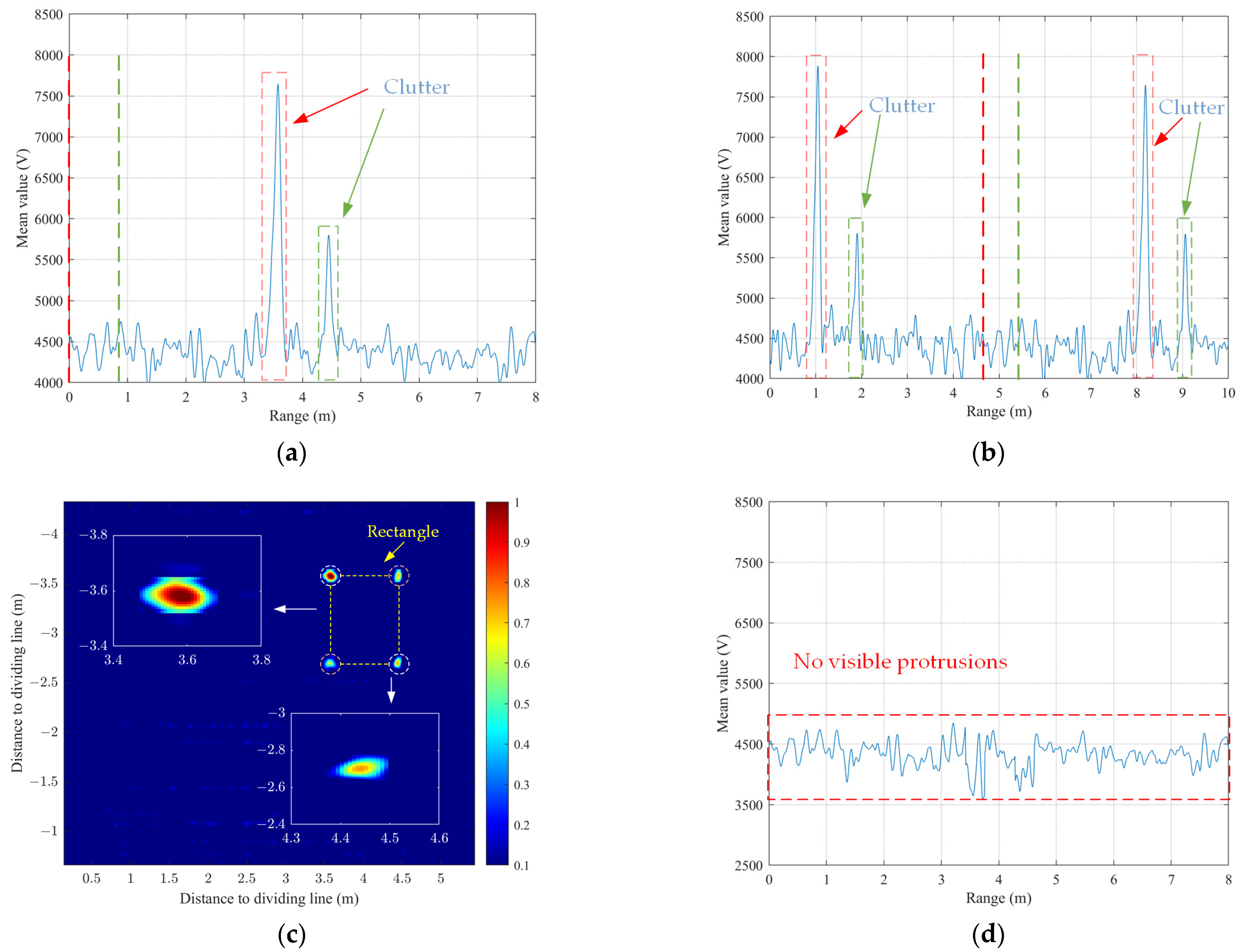
5.1. Free Space Detection

First, the radar shines directly on a metal wall. The front view and the side view of the experimental scenario are shown in Figure 10. The radar transmits the FMCW, and the frequency range is 1.2 GHz to 3 GHz. Transmitting and receiving antennas use Vivaldi antennas. They are parallel to each other and placed towards the metal wall. In this case, the metal wall is obtained by fixing a large metal plate to the wall of the room. The distance between the metal wall and the center of transmitting and receiving antennas is 0.9 m.

Ideally, the beat signal consists of two parts: the directly coupled wave from the transceiver antenna and the reflected wave from the metal wall. The former is greater than the latter. Because of the phase-locked loop spuriousness in the system, the beat signal contains two pairs of clutter in addition to the two parts. A pair of clutter is generated along with the directly coupled wave, located on both sides of its main lobe. The other pair of clutter is generated along with the reflected wave from the metal wall, located on both sides of its main lobe.

The beat signal is processed according to the steps in Section 3. Only time-varying clutter is left. After accumulating along the slow time, the clutter is highlighted, as shown in Figure 11a. The red dashed axis in Figure 11a is the position of the main lobe of the directly coupled wave from the transceiver antenna, and the green dashed axis is the position of the main lobe of the wave reflected from the metal wall. They are eliminated in the treatment of highlighting the clutter. The locations of the two axes are denoted as $R_{red}=0 \mathrm{m}$, $R_{green}=0.9 \mathrm{m}$. Only two spikes are observed in Figure 11a, which are clutter waves located to the right of the main lobe. The clutter symmetrical to it does not appear. The positions corresponding to the two peaks are denoted as $R_{c1}=3.6 \mathrm{m}$, $R_{c2}=4.5 \mathrm{m}$, respectively.

Accessing long delay lines before the transmitting antenna and after the receiving antenna which has an equivalent range of $\Delta R=4.6 \mathrm{m}$, four peaks are observed, as shown in Figure 11b. The distances corresponding to these four peaks are $R_{d1}=1 \mathrm{m}$, $R_{d2}=1.9 \mathrm{m}$, $R_{d3}=8.2 \mathrm{m}$ and $R_{d4}=9.1 \mathrm{m}$, from left to right. The positions of the two axes become ${R_{red}}^{\prime }=\Delta R$ and ${R_{green}}^{\prime }=R_{green}+\Delta R$. The two pairs of clutter waves are symmetric about each of the two axes, i.e., ${R_{red}}^{\prime }=\frac{R_{d1}+R_{d3}}{2}$, ${R_{green}}^{\prime }=\frac{R_{d2}+R_{d4}}{2}$. And the distances of the left and right sides clutter to the corresponding symmetry axes are both equal to $R_x=3.6 \mathrm{m}$.

Using the proposed method, the result obtained by calculating the correlation coefficients of this range-slow time matrix by rows is shown in Figure 11c. Four bright spots appear, arranged in a rectangular shape. The primary diagonal is the correlation coefficient between pairs of clutter before and after. The secondary diagonal is the correlation coefficient between different pairs of clutters. The result shows that the strongest correlation is between pairs of clutter before and after, and there is also some correlation between different pairs of clutter. Figure 11d shows the result after clutter removal using the proposed method. There are no more visible protrusions, indicating that the clutter has been removed.

Additionally, the radar is moved backward in steps of 0.3 m away from the metal wall. As the metal wall becomes farther away from the radar, the position of the main lobe of its echo moves backward and the amplitude becomes weaker. The clutter waves located on either side of it are similarly shifted backward and become weaker. When the distance between antennas and the metal wall is far enough, the clutter is drowned in background noise. Therefore, the range of distances at which the presence of clutter generates false alarms can be measured by varying the distance between antennas and the metal wall. When the radar moves back to a spacing of ${(R_{green})}_{\max }=3.3 \mathrm{m}$ from the metal wall, the clutter on both sides of the main lobe of the metal wall echo is so weak that it is submerged in the background noise. At this point, the green axis in Figure 11b moves to the position of ${({R_{green}}^{\prime })}_{\max }={(R_{green})}_{\max }+\Delta R$. Therefore, ${({R_{green}}^{\prime })}_{\max }=7.9 \mathrm{m}$ is the maximum range at which clutter from a strongly reflected target like a metal wall cannot be ignored. At this limit, the position of the green clutter is on the left if ${({R_{green}}^{\prime })}_{\max }-R_x<{R_{red}}^{\prime }$. This means that the farthest position of the left clutter generated by the strongly reflected target still remains to the left of the red axis. Therefore, the left half of the clutter is located to the left of the dividing line and the right half is located to the right of the dividing line. It ensures that the correlation of a pair of symmetric clutter can be calculated. This verifies the correctness of the proposed method to divide the matrix with the boundary of this position.

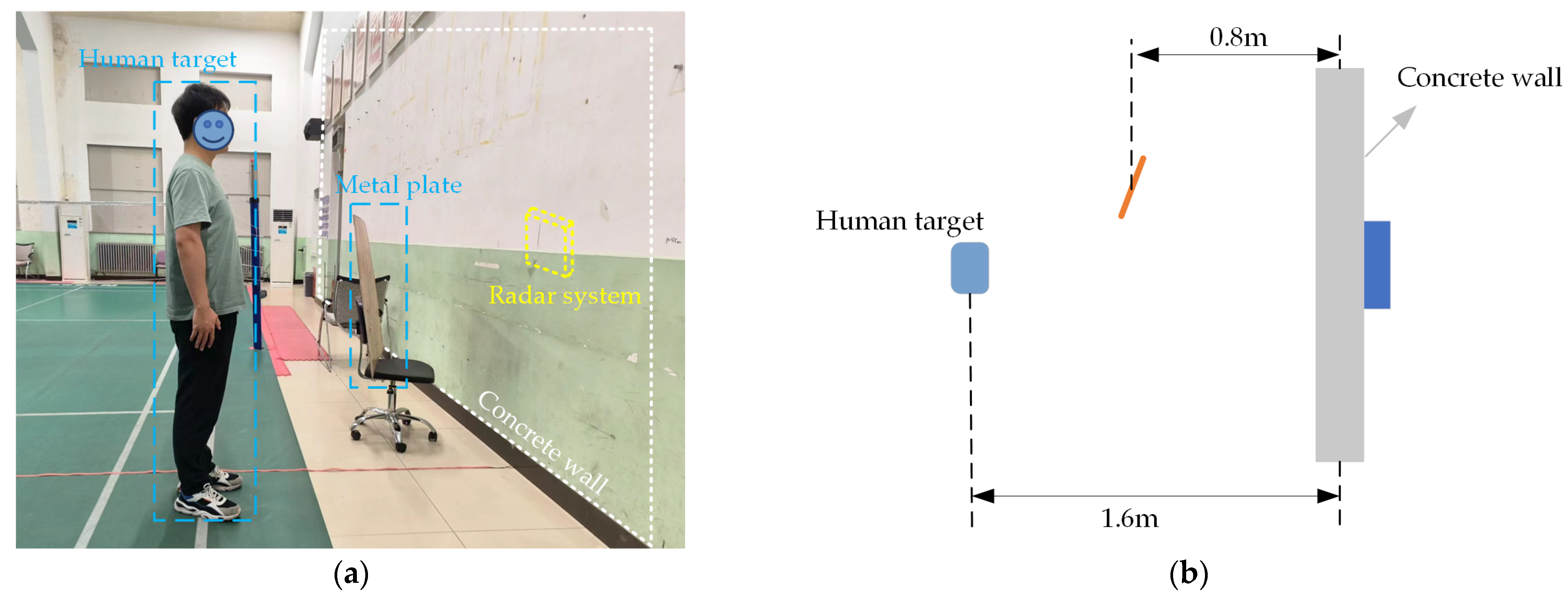
5.2. Through-Wall Detection

The photo and the top view of the experimental scenario for through-wall detection is shown in Figure 12. A concrete wall separates the radar from the targets. The concrete wall is made of solid bricks cast in cement. The thickness and relative permittivity of the concrete wall used are 0.37 m and 4, respectively. The radar is placed against the outside of the wall, and a human body is standing stationary facing the radar at the distance of 1.6 m from the inside of the wall. A square metal plate is placed to the left of the radar and its direct distance from the inside of the wall is 0.8 m. The metal plate is used to simulate the echo from a strongly reflected stationary target. In this case, the components of the beat signal include the directly coupled wave from the transceiver antenna, the reflected wave from the inner wall, the reflected wave from the metal plate, and the reflection from the stationary human target. The reflected wave from the inner wall is the strongest. Because of the presence of phase-locked loop spuriousness, clutter is generated on both sides of the first three echoes.

The reflection from the inner wall is the strongest, so the position of the main lobe of the echo from the inner wall is taken as the coordinate origin. The beat signal is processed according to the steps in Section 3. The main lobe of each echo that does not vary with time is eliminated, while the vital signal of the human target and clutter that vary with time are left. After accumulating along the slow time, the clutter is highlighted, as shown in Figure 13a. As can be seen from the figure, in addition to the vital signal from the human target, clutter is present at three other locations. They seriously interfere with the detection of the vital signal, causing false alarms. After accessing long delay lines which have an equal length of 4.6 m, the symmetrical parts of these clutters are revealed, as shown in Figure 13b. The clutter from the reflected wave from the inner side of the wall is the largest, as shown in the red dashed box. They are symmetric about the red dashed line which corresponds to 4.6 m. The other two pairs of clutter are generated by the directly coupled wave of the transceiver antenna and the echo of the metal plate, respectively. The range-slow time matrix is divided into upper and lower parts according to the dividing line with a range equal to 4.6 m.

Using the calculation of the proposed correlation coefficient, the results are obtained as shown in Figure 13c. The horizontal and vertical axes represent the difference in range between the rows of the two matrices and the dividing line, respectively. A strong correlation between the before and after of paired clutter signals is evident from the main diagonal. Other highlights show that there is also some correlation between unpaired clutter. However, there is no correlation between the clutter and the vital signal. Using the proposed method, the location of the clutter is recognized and then eliminated. Figure 13d shows that the clutter is eliminated clearly and only the vital signal is left.

6. Conclusions

This paper analyzes the effects of periodic nonlinearity during frequency modulation and phase-locked loop spuriousness during frequency division on the beat signal of the FMCW radar. The results of the closed-loop experiments prove that the clutter in the radar system used is generated by phase-locked loop spuriousness. A clutter identification and removal method based on long delay lines and cross-correlation is proposed. The experiments in free space and through-wall detection verify the effectiveness of the proposed method. As for the specific statistical characterization of the amplitude of the clutter generated by phase-locked loop spuriousness, it needs to be studied further.

References

1. Pisa, S.; Pittella, E. A survey of radar systems for medical applications. IEEE Aerosp. Electron. Syst. 2016, 31, 64–81. [Google Scholar] [CrossRef]
2. Regev, N.; Wulich, D. Remote sensing of vital signs using an ultrawide-band radar. Int. J. Remote Sens. 2019, 40, 6596–6606. [Google Scholar] [CrossRef]
3. Gu, C.; Li, C. Assessment of human respiration patterns via noncontact sensing using Doppler multi-radar system. Sensors 2015, 15, 6383–6398. [Google Scholar] [CrossRef] [PubMed]
4. Pramudita, A.A.; Suratman, F.Y. Low-power radar system for noncontact human respiration sensor. IEEE Trans. Instrum. Meas. 2021, 70, 1–15. [Google Scholar] [CrossRef]
5. Seng, C.H.; Bouzerdoum, A. Two-stage fuzzy fusion with applications to through-the-wall radar imaging. IEEE Geosci. Remote Sens. Lett. 2013, 10, 687–691. [Google Scholar] [CrossRef]
6. Becquaert, M.; Cristofani, E. Online sequential compressed sensing with multiple information for through-the-wall radar imaging. IEEE Sens. 2019, 19, 4138–4148. [Google Scholar] [CrossRef]
7. Zhang, D.; Kurata, M. FMCW radar for small displacement detection of vital signal using projection matrix method. Int. J. Antennas. Propag. 2013, 2013, 571986. [Google Scholar] [CrossRef]
8. Wang, S.; Pohl, A. A novel ultra-wideband 80 GHz FMCW radar system for contactless monitoring of vital signs. In Proceedings of the 2015 37th Annual International Conference of the IEEE Engineering in Medicine and Biology Society (EMBC), Milan, Italy, 25–29 August 2015. [Google Scholar] [CrossRef]
9. Pramudita, A.A.; Suratman, F. Modified FMCW system for non-contact sensing of human respiration. J. Med. Eng. Technol. 2020, 44, 114–124. [Google Scholar] [CrossRef] [PubMed]
10. Beasley, P.D.L.; Stove, A.G. Solving the problems of a single antenna frequency modulated CW radar. In Proceedings of the IEEE International Conference on Radar, Arlington, VA, USA, 7–10 May 1990. [Google Scholar] [CrossRef]
11. Ayhan, S.; Scherr, S.A. Impact of Frequency Ramp Nonlinearity, Phase Noise, and SNR on FMCW Radar Accuracy. IEEE Trans. Microw. Theory Technol. 2016, 64, 3290–3301. [Google Scholar] [CrossRef]
12. Park, H.G.; Kim, B. VCO nonlinearity correction scheme for a wideband FMCW radar. Microw. Opt. Technol. Lett. 2000, 25, 266–269. [Google Scholar] [CrossRef]
13. Mizutani, H.; Tsuru, M. A millimeter-wave highly linear VCO MMIC with compact tuning voltage converter. In Proceedings of the 2006 European Microwave Conference, Manchester, UK, 10–15 September 2006. [Google Scholar] [CrossRef]
14. Gomez-Garcia, D.; Leuschen, C. Linear chirp generator based on direct digital synthesis and frequency multiplication for airborne FMCW snow probing radar. In Proceedings of the 2014 IEEE MTT-S International Microwave Symposium, Tampa, FL, USA, 1–6 July 2014. [Google Scholar] [CrossRef]
15. Frischen, A.; Hasch, J. FMCW ramp non-linearity effects and measurement technique for cooperative radar. In Proceedings of the 2015 European Radar Conference, Paris, France, 9–11 September 2015. [Google Scholar] [CrossRef]
16. Meta, A.; Hoogeboom, P. Signal processing for FMCW SAR. IEEE Trans. Geosci. Remote Sens. 2007, 45, 3519–3532. [Google Scholar] [CrossRef]
17. Yang, J.; Liu, C. Nonlinearity correction of FMCW SAR based on homomorphic deconvolution. IEEE Geosci. Remote Sens. Lett. 2013, 10, 991–995. [Google Scholar] [CrossRef]
18. Anghel, A.; Vasile, G.R. Short-range wideband FMCW radar for millimetric displacement measurements. IEEE Trans. Geosci. Remote Sens. 2014, 52, 5633–5642. [Google Scholar] [CrossRef]
19. Wang, R.; Xiang, M. Nonlinear Phase Estimation and Compensation for FMCW Ladar Based on Synchrosqueezing Wavelet Transform. IEEE Geosci. Remote Sens. Lett. 2020, 18, 1174–1178. [Google Scholar] [CrossRef]
20. Jin, K.; Lai, T. A method for nonlinearity correction of wideband FMCW radar. In Proceedings of the 2016 CIE International Conference on Radar, Guangzhou, China, 10–13 October 2016. [Google Scholar] [CrossRef]
21. Levantino, S.; Marzin, G. A Wideband Fractional-N PLL with Suppressed Charge-Pump Noise and Automatic Loop Filter Calibration. IEEE J. Solid-State Circuits 2013, 48, 2419–2429. [Google Scholar] [CrossRef]
22. Ferriss, M.; Plouchart, J.O. An Integral Path Self-Calibration Scheme for a Dual-Loop PLL. IEEE J. Solid-State Circuits 2013, 48, 996–1008. [Google Scholar] [CrossRef]
23. Xue, J.H.; Titterington, D.M. T-Tests, F-Tests and Otsu’s Methods for Image Thresholding. IEEE Trans. Image Process. 2011, 20, 2392–2396. [Google Scholar] [CrossRef] [PubMed]
Figure 1. Free space wave propagation.
Applsci 14 01299 g001
Figure 2. The generation of the spectrum of the beat signal. (a) The ideal frequencies of the transmitted signal (solid line) and received signal (dashed line); (b) The ideal frequency of the beat signal; (c) The ideal spectrum of the beat signal; (d) The frequencies of the transmitted signal (solid line) and received signal (dashed line) under the influence of periodic nonlinearity; (e) The frequency of the beat signal under the influence of periodic nonlinearity; (f) The spectrum of the beat signal under the influence of periodic nonlinearity.
Applsci 14 01299 g002
Figure 3. The variation of  J 0 J 1 J 2  and  J 3  with  τ .
Applsci 14 01299 g003
Figure 4. Schematic diagram of the phase-locked loop (PFD = phase frequency detector, LP = low-pass filter, VCO = voltage-controlled oscillator, 1/N = fractional-N frequency synthesizer).
Applsci 14 01299 g004
Figure 5. Equipment for closed-loop experiments. (a) The physical picture of the radar system used; (b) The physical picture of the optical fibers and corresponding conversion modules; (c) The specific connection between the radar system and the fiber optic module.
Applsci 14 01299 g005aApplsci 14 01299 g005b
Figure 6. Results of closed-loop experiments on an optical fiber with a length of 24 m. (a) The initial range-slow time matrix; (b) The range-slow time matrix with only clutter remaining; (c) The distribution of clutter along the distance.
Applsci 14 01299 g006
Figure 7. Results of closed-loop experiments. (a) The clutter in experiments with optical fibers of different lengths; (b) Changes in the amplitude and position of the clutter. Four points on the same folded line correspond from left to right to the length of the fiber as 12 m, 16 m, 24 m and 40 m.
Applsci 14 01299 g007
Figure 8. Composition of echo signals in through-wall scenarios.
Applsci 14 01299 g008
Figure 9. The specific operation of cross-correlation.
Applsci 14 01299 g009
Figure 10. The experimental scenario in free space. (a) The front view of the experimental scenario; (b) The side view of the experimental scenario.
Applsci 14 01299 g010
Figure 11. Identification and removal of the clutter in free space. (a) The distribution of unprocessed clutter along the distance; (b) Symmetrical clutter after connecting long delay lines; (c) The correlation coefficient matrix; (d) The result after removing clutter.
Applsci 14 01299 g011
Figure 12. The experimental scenario of through-wall detection. (a) The photo of the experimental scenario; (b) The top view of the experimental scenario.
Applsci 14 01299 g012
Figure 13. Identification and removal of the clutter in through-wall detection. (a) The distribution of unprocessed clutter along the distance; (b) Symmetrical clutter after connecting long delay lines; (c) The correlation coefficient matrix; (d) The result after removing clutter.
Applsci 14 01299 g013
Disclaimer/Publisher’s Note: The statements, opinions and data contained in all publications are solely those of the individual author(s) and contributor(s) and not of MDPI and/or the editor(s). MDPI and/or the editor(s) disclaim responsibility for any injury to people or property resulting from any ideas, methods, instructions or products referred to in the content.