Abstract
Dynamic time warping estimates the alignment between two sequences and is designed to handle a variable amount of time warping. In many contexts, it performs poorly when confronted with two sequences of different scale, in which the average slope of the true alignment path in the pairwise cost matrix deviates significantly from one. This paper investigates ways to improve the robustness of DTW to such global time warping conditions, using an audio–audio alignment task as a motivating scenario of interest. We modify a dataset commonly used for studying audio–audio synchronization in order to construct a benchmark in which the global time warping conditions are carefully controlled, and we evaluate the effectiveness of several strategies designed to handle global time warping. Among the strategies tested, there is a clear winner: performing sequence length normalization via downsampling before invoking DTW. This method achieves the best alignment accuracy across a wide range of global time warping conditions, and it maintains or reduces the runtime compared to standard usages of DTW. We present experiments and analyses to demonstrate its effectiveness in both controlled and realistic scenarios.
1. Introduction
Dynamic time warping (DTW) is a dynamic programming algorithm that calculates the optimal alignment between two sequences under certain assumptions. Though designed to handle an unknown amount of time warping, in practice DTW’s performance often degrades when the two sequences differ substantially in scale [1,2,3], resulting in a global time warp factor that deviates from one. Scale differences arise naturally in many domains: query-by-humming systems must handle singing at different tempos [4], gait recognition involves different walking speeds [5], query-by-sketch systems must handle differences in scale [6], and similar issues arise in multimedia [7] and bioinformatics [8]. This paper studies the effect of global time warping conditions on the alignment accuracy of DTW in a systematic manner and experimentally explores several ways to improve the robustness of DTW to varying levels of global time warping. To make our study concrete, we will focus on an audio–audio alignment scenario in which the goal is to accurately estimate the temporal alignment between two different audio recordings of the same piece of music (e.g., two different piano performances of a composition).
Previous works on DTW generally fall into one of four groups. The first group focuses on speeding up exact DTW (or subsequence DTW), often in the context of a database search. This has been accomplished in many ways, including lower bounds [9,10], early abandoning [11,12], parallelizing across multiple cores [13,14], or using specialized hardware [15,16]. Several recent works have utilized GPUs to reduce the runtime of computing exact DTW on long sequences [17,18]. The second group focuses on reducing the quadratic memory and computation costs through approximations of DTW. These include approximate lower bounds [19,20], imposing bands in the cost matrix to limit severe time warping [21,22], performing alignments at multiple different resolutions [23,24], parallelizable approximations of DTW [18,25], and estimating alignments within strict memory limitations [26]. The third group focuses on extending the behavior of DTW to make it more flexible. Examples in the music information retrieval literature include handling structural differences due to repeats or jumps in music [27,28,29], aligning sequences in an online setting [30,31,32], handling partial alignments [33,34], utilizing multiple performances of a piece to improve alignment accuracy [35], and handling pitch drift in a capella music [36]. The fourth group focuses on integrating DTW into modern neural network models. These include differentiable approximations of DTW suitable for backpropagation [37,38,39] or adopting a hard alternating scheme [40,41,42]. We note that our present study falls into the third group (more flexible behavior), as our focus is on improving robustness under certain conditions.
This paper poses the following question: “How can we make DTW more robust to global time warping conditions?” There are two practices that are commonly used to handle differences in scale. The first practice is to select an appropriate set of allowable transitions to handle the amount of expected time warping. For example, the set allows for a maximum time warping factor of 2, while the set theoretically allows for an infinite amount of time warping. This is a design decision that must be made whenever DTW is invoked. The second practice is to re-scale the sequences to be the same length before invoking DTW [1,2]. Though these two practices are commonly adopted, we are not aware of any studies that systematically study their effectiveness as a function of the global time warping factor. This paper compares these two approaches—and others—to determine how well they perform across a range of global time warping conditions. To study this question in a systematic manner, we adopt a dataset commonly used to study audio synchronization, modify it to construct benchmarks in which the average global time warping conditions are carefully controlled, and then use our controlled benchmarks to study the effectiveness of several strategies for handling global time warping. Our goal is to understand the effect of global time warping on the alignment accuracy of DTW and to identify a set of best practices for handling varying global time warping conditions.
This paper has three main contributions. First, we introduce a framework for systematically studying the effect of global time warping conditions in an audio–audio alignment task. Second, we explore several ways to improve the robustness of DTW to varying levels of global time warping, and we characterize their effectiveness in our controlled benchmarks. Third, we provide a clear recommendation for best practice in handling global time warping conditions: sequence length normalization with downsampling. This method achieves the best alignment accuracy across a wide range of global time warping conditions, while maintaining or reducing runtime compared to standard usages of DTW. Code for reproducing our experiments can be found at https://github.com/HMC-MIR/ExtremeTimeWarping (accessed on 5 February 2024).
The rest of the paper is organized as follows. Section 2 introduces four different methods for handling or mitigating the effect of global time warping. Section 3 describes our experimental setup to study the effect of global time warping under controlled conditions and presents our empirical results and findings. Section 4 conducts two additional analyses to gain a deeper insight into the results. Section 5 concludes the work.
2. Materials and Methods
In this section, we describe several methods for dealing with global time warping. First, we explain the standard DTW algorithm for completeness, and then we describe four different ways to handle global time warping.
Standard DTW estimates the alignment between two sequences , , … and , , …, in the following manner. First, a pairwise cost matrix is computed, where indicates the distance between and under a particular cost metric (e.g., Euclidean distance, cosine distance). Next, a cumulative cost matrix is computed with dynamic programming, where indicates the optimal cumulative path cost from to under a pre-defined set of allowable transitions and transition weights. For example, with a set of allowable transitions {, , } and corresponding transition weights {2, 3, 3}, the elements of D can be computed using the following recursion:
During this dynamic programming stage, a backtrace matrix is also computed, where indicates the optimal transition ending at . Once D and B have been computed using dynamic programming, we can determine the optimal path through the cost matrix by following the backpointers in B starting at position . The optimal path defines the predicted alignment between the two sequences.
2.1. Different Transitions and Weights
One obvious way to deal with global time warping is to simply select a set of allowable transitions to explicitly handle a specified amount of time warping. This is a design decision that must be made whenever DTW is invoked. For example, the transition set can theoretically handle an infinite amount of time warp. In practice, however, these transitions often lead to degenerate alignments and unstable or undesirable behavior. A more conservative way to handle global time warping is use transitions like and , which limit the maximum amount of time warping that can be handled. A commonly used set of transitions in the audio synchronization literature is {, , }, which imposes a maximum allowable time warp factor of 2. In a similar manner, the set of transitions {, , , , } imposes a maximum allowable time warp factor of 3, and the set {, , , , , , } imposes a maximum allowable time warp factor of 4. These additional transitions come with a significant computational cost, however, since each step of the dynamic programming stage needs to consider every possible transition (cf. Equation (2)). In Section 3 and Section 4, we will compare both the alignment accuracy and the runtime of several different settings for transition types and weights.
2.2. Normalizing Sequence Length
Another common way to deal with global time warping is to normalize the sequence lengths before estimating the alignment. This technique has been explored in many forms in previous works [43,44,45]. Let , , …, and , , …, be the two sequences that we would like to align, where . Before computing the pairwise cost matrix C, we can downsample the sequence , , …, to match the length of the other sequence, yielding a modified sequence , , …, . One simple way to perform this downsampling is to simply calculate a weighted combination of the two nearest neighbors. In this approach, we first create N linearly spaced indices between 0 and , and then use these indices to compute values as a weighted combination. For example, a desired sample at index would be calculated as . Once both sequences have been normalized in length, we can use standard DTW to estimate the alignment between , , …, and , , …, , and then account for the global downsampling factor to infer the alignment between , , …, and , , …, .
There are multiple ways one might normalize sequence length. In our experiments, we consider two different dimensions of behavior. One dimension is to either (a) downsample the longer sequence to match the length of the shorter sequence, or (b) upsample the shorter sequence to match the length of the longer sequence. The second dimension is to perform upsampling/downsampling by either (a) using linear interpolation between the two nearest neighbors (as described in the previous paragraph) or (b) simply using the nearest neighbor (e.g., a desired sample at index would be represented as ). In Section 3 and Section 4, we characterize the performance and runtime of the four possible combinations: downsampling with linear interpolation, downsampling with nearest neighbor, upsampling with linear interpolation, and upsampling with nearest neighbor.
2.3. Adaptive Weighting Schemes
A third way to deal with severe time warping is to select transition weights adaptively during the run time rather than using a fixed set of transition weights tuned on a training set. Let , , …, and , , …, be the two sequences that we would like to align, where . If we use standard DTW with allowable , transitions {, } and corresponding weights {, }, then we can adaptively set and for each pair of sequences to be aligned. This weighting scheme ensures that both axes contribute the same weighted Manhattan distance cost from to , regardless of the values of N and M. (Note that if , the axis along the shorter sequence contributes less to the total path cost simply because it is shorter in length.) This prevents one axis from dominating the total path cost. Similarly, we can use standard DTW with allowable , transitions {, , } and corresponding weights {, , }, where we can adaptively set , , and . This preserves the property that both axes contribute equally to the total path cost, and it allows transitions as well.
2.4. Non-Uniform Transition Patterns
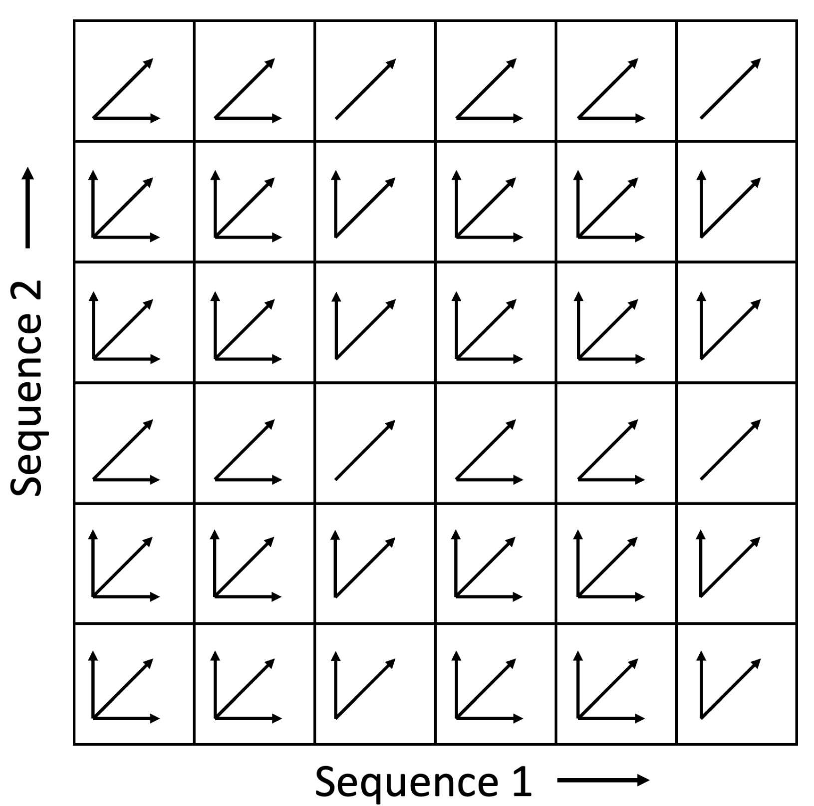
A fourth way to deal with severe time warping is to use non-uniform transition patterns at different positions in the cost matrix. This approach is identical to standard DTW except that the set of allowable transitions at each position in the pairwise cost matrix may be different. Consider a nominal set of allowable transitions {, , } with corresponding weights {1, 1, 2} and a desired maximum time warping factor . If we remove the transition from all positions where , and likewise remove the transition from all positions where , then we effectively impose a maximum time warping factor of . Figure 1 shows an illustration of the case when . The benefit of this approach is that it can handle more extreme time warping, but it limits horizontal/vertical degenerate paths and avoids the computational cost of adding additional transition types.

Figure 1.
An example of a pairwise cost matrix in which the set of allowable transitions at each position is different. The pattern shown above assumes nominal transitions of , , and , but where transitions are removed in every third row and transitions are removed in every third column. The resulting pattern allows for a maximum time warping factor of 3.
In Section 3, we will characterize how effective the above methods are in dealing with varying global time warping conditions.
3. Results
In this section, we describe how we constructed a benchmark to perform a controlled study on the effects of global time warping (Section 3.1), and then share the results of our experimental study (Section 3.2).
3.1. Experimental Setup
Our benchmark is a modification of the Mazurka Dataset [46]. The Mazurka Dataset contains historic audio recordings of five Chopin Mazurkas, along with beat-level annotations. This dataset has been used to study various audio-related tasks that require precise timing information, such as audio synchronization, beat tracking, and tempo estimation (e.g., [18,35,47,48]). Table 1 shows the number of recordings for each Mazurka and descriptive statistics for the recording duration. For each Mazurka, every possible pairing of recordings is considered, the two recordings are aligned, and the predicted alignment is compared to the ground truth annotations to evaluate alignment accuracy. Note from Table 1 that the global time warping conditions in the original dataset range from 1 to (between the longest and shortest recordings for Opus 63, No 3). We set aside the Op. 17 No. 4 and Op. 63 No. 3 Mazurkas for training/development and used the remaining three Mazurkas for testing. Because our interest in this work is in the alignment algorithm, in all experiments we simply use standard chroma features and a cosine distance metric. For computing chroma features, we used librosa [49] with default settings: 22,050 Hz sampling rate, 512 sample hop length, and spanning seven octaves between C1 and C8.

Table 1.
Overview of the original Chopin Mazurka dataset [46]. This is used as the source data to generate a benchmark suite in which the global average time warping factor is controlled. The top two pieces are used for training and the bottom three pieces are used for testing. All durations are in seconds.
We created seven different modified versions of the Mazurka Dataset. Our goal was to construct datasets that would allow us to measure alignment accuracy across a wide range of carefully controlled global time warping conditions. The modified datasets were constructed in the following manner. First, for each Mazurka, we calculated the median duration of all recordings, which we denote as . In Table 2, the values for each Mazurka are indicated in the column labeled “×1.000”. Second, we determined a set of seven target durations: , , , , , , and . Note that these target durations are spaced evenly on a log scale and span a factor of . Finally, we time-scale modified each individual recording to its target durations, and also modified the beat annotations accordingly. Time-scale modification (TSM) is a technique in which the tempo (and thus duration) of a piece of music is altered without changing the pitch. We used the approach described in [50], in which the audio waveform is first separated into percussive and harmonic components, the percussive component is time-scale modified with a basic overlap-add method, the harmonic component is time-scale modified with a phase vocoder [51], and the resulting time-scale modified components are added. (Note that most existing implementations of TSM use a hop size that is rounded to the nearest audio sample, which results in an effective TSM factor that is slightly different than what is specified. Because we wanted precise control over the recording durations, we implemented our TSM from scratch, including a re-implementation of the STFT function that allows for a non-integer hop size in samples.) The end result of this process is a set of seven different versions of the Mazurka Dataset, which we refer to as median_x0.500, median_x0.630, median_x0.794, median_x1.000, median_x1.260, median_x1.588, and median_x2.000. Table 2 provides an overview of these modified datasets. In each of these seven datasets, all of the recordings of the same Mazurka have exactly the same duration. So, for example, in the median_x2.000 dataset, all of the Op. 30 No. 2 recordings are approximately 174.6 seconds in duration.
Table 2.
Overview of the modified Mazurka Datasets. We constructed seven modified versions of the Mazurka Dataset to study alignment accuracy under controlled global time warping conditions. All recordings of the same Mazurka are time-scale modified to a target duration, where target durations are calculated as the median duration multiplied by a constant scaling factor (0.500, 0.630, 0.794, 1.000, 1.260, 1.588, 2.000). Recording durations for the seven modified datasets are shown in the table and are expressed in seconds.
We then ran experiments by considering pairs of modified datasets, as shown in Table 3. Each pairing of datasets constitutes a benchmark with a fixed average global time warp factor, where the global time warp factors range between and . Note that there are multiple different pairings of modified datasets that could achieve the same fixed global time warp factor. Among the possible pairings, we adopted the strategy of pairing a dataset that is “sped up” with a dataset that is “slowed down”, in order to minimize artifacts from performing TSM with extreme factors. For each pairing of datasets, we then ran an experiment exactly as before: we considered every possible pair of audio recordings of the same Mazurka (where A is taken from one modified dataset and B is taken from the other modified dataset), aligned the pair of recordings, and then evaluated the accuracy of the predicted alignment. Note that, in each of the seven benchmarks described above, we have exactly the same number of recording pairs as in the original Mazurka Dataset benchmark: pairs for training and pairs for testing. The difference is that in each pairing of recordings , the durations of A and B have been modified via TSM to achieve a fixed global time warping factor. For example, when pairing the median_x2.000 and median_x0.500 datasets, every pair of recordings from Opus 17 No 4 will have a global average time warping factor of , and every pair of recordings from Opus 24 No 2 will also have a global average time warping factor of , etc.
Table 3.
The pairings of modified Mazurka Datasets used to study fixed global time warping ratios. For example, to study performance at a global time warping ratio of 2, we consider pairs of audio recordings where A is selected from the median_x1.588 dataset and where B is selected from the median_x0.794 dataset.
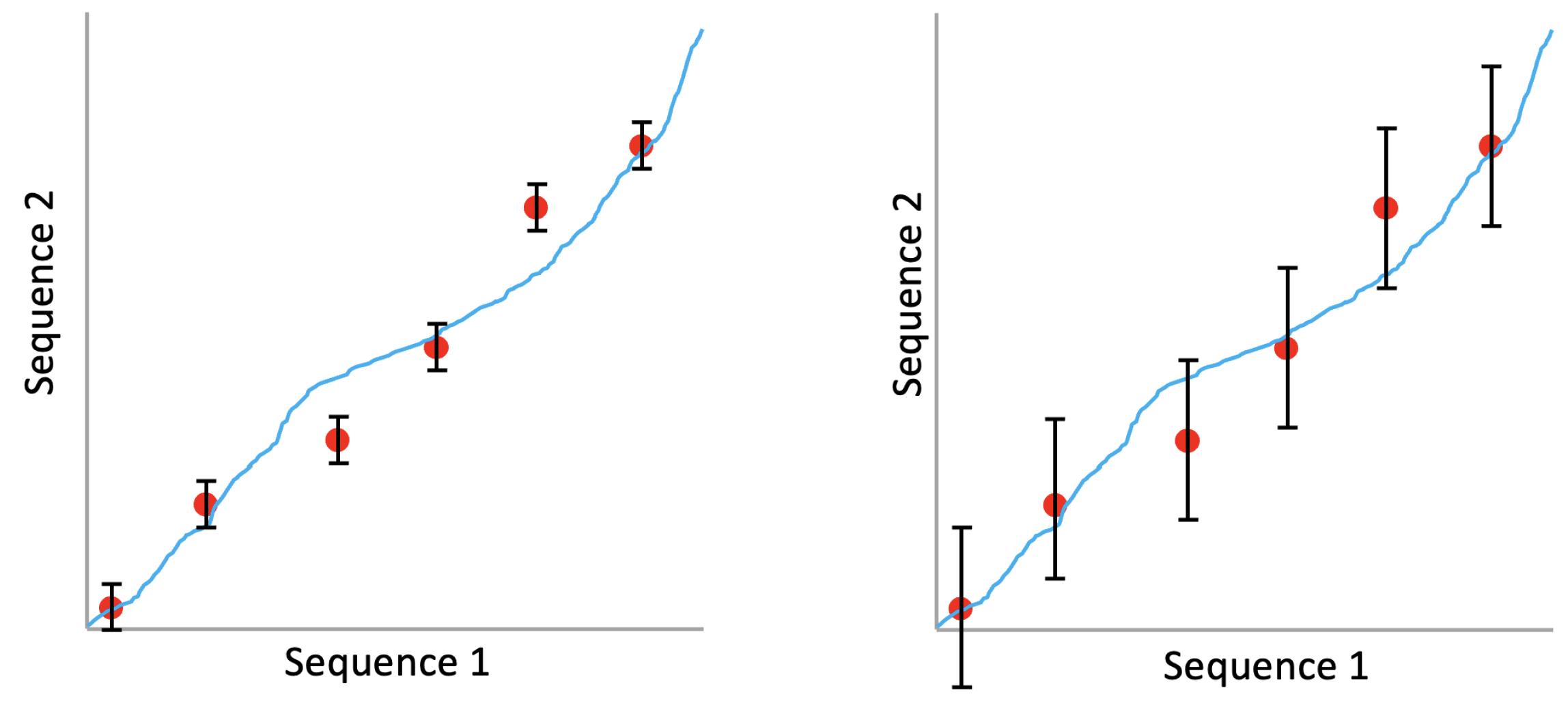
We evaluate alignment accuracy in the following manner. Given a predicted alignment between two recordings A and B, we determine the predicted timestamp in B that corresponds to each ground truth beat timestamp in A. The difference between the predicted timestamp in B and the actual ground truth beat timestamp in B is the alignment error. We can then calculate the percentage of predictions that are incorrect (error rate), where we define an incorrect prediction as one that has an alignment error greater than a fixed threshold value (error tolerance). Thus, there is a tradeoff between error rate and error tolerance. Figure 2 shows the process of calculating the error rate for a predicted alignment with two different error tolerances. With a small error tolerance (left), two out of six beat timestamps are considered incorrect, resulting in an error rate of . With a larger error tolerance (right), all six beat timestamps are considered correct, resulting in an error rate of . In our experimental results in Section 3, error rates are computed across all predicted alignments in the benchmark, and we report error rates at multiple different error tolerances.
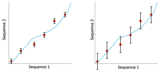
Figure 2.
Example showing how we evaluate alignment accuracy. Red points indicate ground truth beat timestamps, the blue trajectory indicates a predicted alignment, and the black vertical bars indicate error tolerance. With a small error tolerance (left), the error rate is . With a larger error tolerance (right), the error rate for the same predicted alignment is . We report error rates at multiple error tolerances.
There is one subtle yet very important detail regarding evaluation. Consider the evaluation of a predicted alignment between two recordings A and B. At the ground truth beat timestamp in A, let us say that the predicted alignment error in B is 50 ms. If we take the exact same predicted alignment but elongate the time axis in B by a factor of two, the predicted alignment error in B will be 100 ms. Clearly, the predicted alignment has not gotten any worse in quality—it has simply been projected into a time axis that is elongated. To account for this issue, when calculating the alignment error, we project all predicted alignments into the median_x1.000 time axis and then apply a fixed error tolerance. This ensures that alignment errors in different time scales are compared fairly. One way to think about this is that we are using an error tolerance that is (roughly) a fixed fraction of a musical beat, rather than a fixed absolute duration of time.
3.2. Experimental Results
We evaluated the performance of 17 alignment algorithms. The first seven systems explore the use of different transition types and weights for standard DTW, as described in Section 2.1. The next four systems explore the use of sequence length normalization, as described in Section 2.2. The next two systems explore the use of adaptive weighting schemes, as described in Section 2.3. The last four systems explore the use of non-uniform transition patterns, as described in Section 2.4. Table 4 defines each of these 17 systems, grouped into the four categories described above. We ran experiments with many other variants and only included the best-performing ones in the 17 listed in the table. For example, we tried applying sequence length normalization to other transition and weighting schemes, but only present results with DTW2 since it yielded the best results. Likewise, we considered several other weighting schemes with standard DTW, but only present the best-performing ones.
Table 4.
Explanation of the 17 systems whose performance is compared in Figure 3. Systems are grouped into four different categories: standard DTW, sequence normalization, adaptive weighting, and selective transitions.
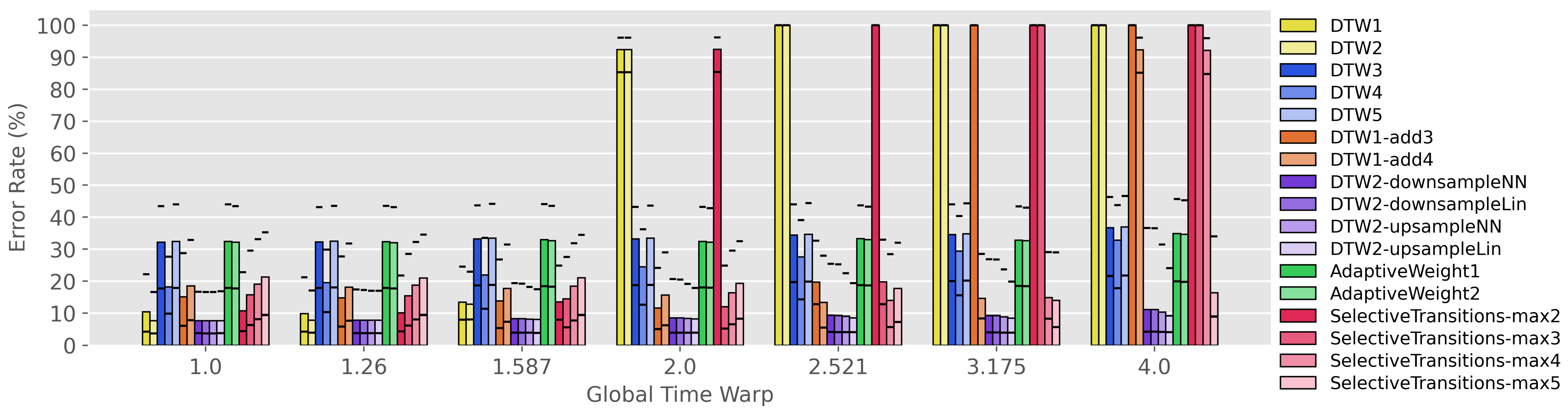
Figure 3 shows the alignment accuracy of all 17 alignment methods on our benchmarks. The seven groups along the horizontal axis correspond to the seven different benchmarks, where each benchmark has an average global time warping factor between 1.0 and 4.0. Within each group, the colored bars correspond to the 17 different alignment methods. Note that bar colors have been chosen to group similar alignment methods together, so that variations of the same method are indicated with a gradient of the same hue. Each individual bar indicates the error rate at an error tolerance of 200 ms when projected onto the median_x1.000 time scale. On top of each bar, we have also overlaid two horizontal black lines indicating the error rates at tolerances of 100 ms (above) and 400 ms (below). The y-axis indicates error rate, so lower is better.

Figure 3.
Assessing the robustness of various alignment methods to global time warping conditions. The seven groups along the horizontal axis correspond to seven benchmarks with different average global time warping factors. Colored bars indicate the error rate at 200 ms error tolerance, and the black horizontal lines indicate error rate at error tolerances of 100 ms (above) and 400 ms (below). Note that the bar colors are grouped by category, so that similar algorithms are shown as different shades of the same hue.
There are many things to notice about Figure 3. We will unpack and interpret the results for each color group in the paragraphs below.
First, consider the two yellow systems (DTW1, DTW2). These two systems have allowable transitions , , with two different weighting schemes. This set of allowable transitions is often used in audio–audio alignment, so these systems can be interpreted as a type of baseline. We see that both systems have good performance for low global time warp factors, but that performance is terrible for global time warp factors of and higher. This makes intuitive sense, since the set of transitions , , imposes a maximum allowable time warping factor of 2. Thus, we can summarize the performance of our baselines in the following way: they perform well with moderate global time warping (<2), but they cannot handle severe global time warping (≥2) at all.
Second, consider the three blue systems (DTW3, DTW4, DTW5). What these three systems have in common is that they allow and transitions, which theoretically should be able to handle an infinite amount of time warping. Their performance thus addresses the question, “Can we handle severe global time warping by including and transitions in standard DTW?” We can see in Figure 3 that the performance of these systems is relatively invariant to the global time warp factor. For example, the error rate of the DTW3 system only degrades from about 32% to 37% as the global time warp factor increases from to . However, the error rates of all three systems is relatively high, and they do not have competitive performance compared to the other systems under any global time warp conditions. So, the short answer to the question above is: no, adding and transitions is not an effective method of handling severe global time warping.
Third, consider the two orange systems (DTW1-add3, DTW1-add4). These two systems add additional transitions like and to the standard set {, , }. These systems address the question, “Can we handle more severe global time warping conditions by adding more extreme transitions to standard DTW?” We can see in Figure 3 that the performance is degraded for low global time warp factors, but that the two systems are indeed able to cope with more extreme time warping. For example, DTW1-add3 has reasonably good performance for global time warp factors , and DTW1-add4 has reasonably good performance for global time warp factors . However, we must also keep in mind that these systems require more computation, since each step in the dynamic programming stage must consider more possibilities (e.g., seven for DTW1-add4 compared to three for DTW1). So, the short answer to the question above is that adding more extreme transitions can make DTW more robust to severe global time warping, but it comes at a heavy computational cost and a moderate degradation in accuracy.
Fourth, consider the four purple systems (DTW2-downsampleNN, DTW2-downsampleLin, DTW2-upsampleNN, DTW2-upsampleLin). These four systems all perform some form of sequence length normalization before applying DTW with standard settings. We can see in Figure 3 that these four systems have the best performance among all systems across all seven global time warp factors. Furthermore, the performance is largely invariant to the global time warp factor. Interestingly, all four systems have very similar accuracy, with the upsampling variants showing a slight performance benefit at high global time warp factors. Given that upsampling results in much longer sequences (and therefore more computation in performing DTW), the most practical option is DTW2-downsampleNN due to its simplicity. In summary, the sequence length normalization technique is the clear winner among the four methods—it has the best performance across all conditions and is largely invariant to the global time warping factor.
Fifth, consider the two green systems (AdaptiveWeight1, AdaptiveWeight2). These systems have and transitions with weights that are computed at run time based on the lengths of the two sequences. We can see in Figure 3 that these systems have roughly the same behavior as the other systems that include and transitions. The adaptive weighting does not seem to provide additional benefit in handling global time warping conditions.
Finally, consider the four red systems (SelectiveTransitions-max{W} where ). These systems all have , , nominal transitions but selectively remove the and transitions from selected locations in the pairwise cost matrix. We can see in Figure 3 that this scheme does indeed provide robustness to extreme time warping. For example, SelectiveTransitions-max2 has reasonable performance for global time warp factors , SelectiveTransitions-max3 has reasonable performance for global time warp factors , etc. However, compared to the best-performing systems, these variants show a moderate degradation in alignment accuracy. One difference between this approach and DTW1-add3 and DTW1-add4 is the computational cost: since we are removing transitions (rather than adding additional transitions), we do not need to consider as many possibilities and the resulting computational cost is lower (in theory). So, non-uniform transition patterns do seem to make DTW more robust to global time warping conditions, but they come with a moderate reduction in accuracy.
4. Discussion
In this section, we conduct two additional analyses to gain a deeper insight into our experimental results.
The first analysis is to characterize the runtime of different algorithms. We can do this in two ways: a theoretical analysis and an empirical analysis. The theoretical runtime can be considered in the following manner. Let N and M represent the sequence lengths of the two sequences to be aligned, where we assume without loss of generality. Let T represent the number of possible transition types at each location in the cost matrix. Then, the computational complexity of standard DTW is . This applies to the seven systems that explore the use of different transition types and weights (DTW1-5, DTW1-add3, DTW1-add4) and the adaptive weighting schemes (AdaptiveWeight1-2). For the sequence length normalization methods, the computational complexity is when downsampling and when upsampling. For the non-uniform transition patterns, the average number of transition types per location is reduced to , so the computational complexity is .
We used the following procedure to measure the empirical runtime. Given two sequence lengths, N and M, we randomly initialize two feature matrices of size and , where the 12 is selected to simulate a chroma feature representation. We begin profiling after the feature matrices have been generated, and we include feature preprocessing (e.g., downsampling for sequence length normalization), pairwise cost matrix computation, dynamic programming, backtracking, and any postprocessing (e.g., compensating for downsampling). For each setting of , we repeat this process 10 times and report the average runtime. All experiments were run on a 2.1 GHz Intel Xeon processor with 192 GB of DDR4 RAM, and all alignment algorithms are implemented in cython.
Figure 4 compares the runtime of all 17 alignment algorithms. Each group along the horizontal axis corresponds to one setting of , where N and M indicate the lengths of the shorter and longer sequence, respectively. We have included results for 1k, 3k, 10k, 30k, and , , . These settings allow us to see the effect of both the sequence length and the global time warp factor. For ease of viewing, the groups have been split into two subplots. Within each group, the different bars correspond to the 17 alignment algorithms; we use the same color scheme as in Figure 3. The height of each bar indicates the average runtime across 10 runs, where runtime is shown on a log scale. Note that the results for (30k, 120k) are missing for the two upsampling systems—this is because the upsampling approach creates a 120k × 120k pairwise cost matrix and cumulative cost matrix, and this exceeded the RAM limits for our server.
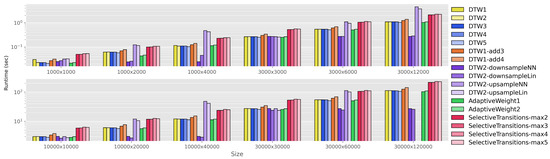
Figure 4.
Comparison of runtimes for aligning two sequences of length N and M, where 1k, 3k, 10k, 30k and , , . This selection of settings allows us to assess the effect of sequence length as well as average global time warping factor. The reported runtimes are the average of 10 trials. Note that the y-axis is shown on a log scale.
There are several things to notice about Figure 4. First, the DTW1 through DTW5 systems have similar runtimes, since all are standard DTW with three allowable transitions. This is a baseline that represents typical DTW usage. Now, we consider the remaining groups. DTW1-add3 and DTW1-add4 (orange) have increased runtimes compared to the baseline, since they require more transition possibilities to be considered at each step of the dynamic programming stage. The sequence normalization methods (purple) have the most interesting runtime trends. When , the runtimes of all four sequence normalization methods are similar to the baseline. However, as the global time warping factor increases, the downsampling variants show a significant decrease in runtime compared to the baseline, while the upsampling variants show a significant increase in runtime. This makes sense: when and , the downsampling variants will perform DTW on a pairwise cost matrix while the upsampling variants will perform DTW on a pairwise cost matrix. The adaptive weighting schemes (green) show similar performance to the baseline, with a decrease in runtime for the variant that only has two allowable transitions. Interestingly, the systems with non-uniform transition patterns (red) show a significant increase in runtime compared to the baselines. While in theory these methods require fewer transition possibilities to be considered, in practice the implementation of non-uniform transition patterns requires additional logic within the nested loops, which results in an increase in runtime.
The main takeaway from our runtime analysis is this: the downsampling sequence normalization methods are the clear winner. They have the best alignment accuracy across all global time warping conditions, and they also have the best runtime characteristics. The runtime of these methods roughly matches standard DTW when , and it substantially reduces the runtime under more extreme global time warping conditions.
The second analysis is a sanity check. We have performed extensive experiments under carefully controlled global time warping conditions, and we have found a clear winner: sequence length normalization with downsampling. But the real question is this: does this method help in practice under real conditions? To answer this question, we compared the performance of the best standard DTW configurations (DTW1, DTW2) with their corresponding sequence normalized methods (DTW1-downsampleNN, DTW1-downsampleLin, DTW2-downsampleNN, DTW2-downsampleLin) on the original Mazurka Dataset. Table 5 compares the error rates of these six systems at three different error tolerances: 100 ms, 200 ms, and 500 ms.
Table 5.
Comparing the error rates of the best standard DTW configurations and the best sequence length normalization methods on the original Chopin Mazurka dataset. Numbers in the table indicate error rate at three different error tolerances.
There are two things to notice about Table 5. First, we see that sequence normalization consistently improves alignment accuracy. This improvement holds across different weighting schemes (DTW1, DTW2) and across all error tolerances. This suggests that the sequence normalization method may be useful as a general best practice, and not just when there is extreme global time warping. Second, we observe that the improvement is more pronounced for larger error tolerances. For example, when applying sequence normalization to DTW2, the error rate at a 100 ms tolerance decreases from 14.1% to 13.2% (a 6.4% reduction in errors), and at a 500 ms tolerance decreases from 3.6% to 2.6% (a 27.8% reduction in errors). Intuitively, we do not expect that downsampling a sequence will greatly improve its fine-grained alignment accuracy since downsampling throws away fine-grained information. But the main effect we are observing here is that sequence normalization reduces the likelihood that the ground truth alignment path will exceed a maximum allowable time warping factor (imposed by the selected set of allowable transitions). This results in a substantial improvement in alignment accuracy at mid- and coarse-level error tolerances.
It is important to point out the limitations of our study. The audio–audio alignment task we have selected has several distinctive characteristics that may limit the generalizability of our findings: (a) sequence elements (e.g., chroma features) have strong correlations over time, (b) sequence elements are continuous valued rather than discrete symbols, and (c) the true alignment path is (roughly) monotonically increasing, meaning that the alignment is a one-to-one mapping (rather than a many-to-one mapping). We cannot say if our conclusions and findings will necessarily generalize to settings in which these characteristics are different. For example, if the sequences consist of discrete tokens with no temporal correlation, then downsampling may have a very different effect. Nonetheless, we are eager to study to what extent these conclusions may generalize to other domains in future work. Furthermore, we also point out that the sequence normalization method has two restrictions. First, it requires knowing the average global time warping factor a priori, usually through a boundary assumption, in which we assume that both sequences begin and end together. For situations like subsequence DTW, in which the boundary conditions are not known a priori, sequence normalization methods cannot be applied. Second, it only provides benefit in handling global (rather than local) time warping conditions. For example, if the true alignment path has an average global time warping factor close to one but contains a local section with extreme time warping, the sequence normalization method will not provide any benefit. This is also an area to explore in future work.
5. Conclusions
We have proposed a framework for studying the effect of global time warping conditions in an audio–audio alignment task. We characterize the behavior of standard usages of DTW, along with several strategies for improving robustness to global time warping. Our main findings are (a) standard usages of DTW perform well when both sequences are comparable in length but completely fail to handle severe global time warping; (b) using and transitions in DTW leads to poor alignment quality and is not an effective solution; (c) several strategies like adding more extreme transitions and using non-uniform transition patterns can improve robustness to global time warping, but come with a computational cost and reduction in alignment quality, and (d) the most effective strategy we found is to perform sequence length normalization using downsampling before invoking DTW. This approach achieved the best alignment accuracy across a wide range of global time warping conditions, while simultaneously maintaining or reducing runtime compared to standard usages of DTW. Because it never degrades performance and may offer substantial improvement in both runtime and accuracy, we recommend using downsampling sequence normalization as a default practice when invoking DTW. For future work, we would like to (a) determine a set of best practices for handling severe time warping conditions in the subsequence DTW case, where the global time warp factor between both sequences is unknown a priori; (b) study to what extent our findings may generalize to other domains with different data characteristics; and (c) further explore the effect of sequence normalization when changing the lengths of both sequences.
Author Contributions
Conceptualization, T.J.T.; Funding acquisition, T.J.T.; Methodology, T.J.T.; Software, J.K. and A.P.; Supervision, T.J.T.; Validation, J.K. and A.P.; Writing—original draft, T.J.T.; Writing—review & editing, J.K. and A.P. All authors have read and agreed to the published version of the manuscript.
Funding
This material is based upon work supported by the National Science Foundation under Grant No. 2144050.
Institutional Review Board Statement
Not applicable.
Informed Consent Statement
Not applicable.
Data Availability Statement
Code for reproducing our experiments can be found at https://github.com/HMC-MIR/ExtremeTimeWarping (accessed on 5 February 2024). The Mazurka Dataset has copyright restrictions and cannot be released publicly.
Acknowledgments
We would like to thank Kavi Dey, Meinard Müller, and Yigitcan Özer for helpful feedback and discussions.
Conflicts of Interest
The authors declare no conflicts of interest. The funders had no role in the design of the study; in the collection, analyses, or interpretation of data; in the writing of the manuscript; or in the decision to publish the results.
Abbreviations
The following abbreviations are used in this manuscript:
| DTW | Dynamic Time Warping |
| GPU | Graphics processing unit |
| RAM | Random access memory |
| STFT | Short-time Fourier transform |
| TSM | Time-scale modification |
References
- Fu, A.W.C.; Keogh, E.; Lau, L.Y.H.; Ratanamahatana, C.A.; Wong, R.C.W. Scaling and time warping in time series querying. VLDB J. 2008, 17, 899–921. [Google Scholar] [CrossRef]
- Shen, Y.; Chen, Y.; Keogh, E.; Jin, H. Accelerating time series searching with large uniform scaling. In Proceedings of the 2018 SIAM International Conference on Data Mining, San Diego, CA, USA, 3–5 May 2018; pp. 234–242. [Google Scholar]
- Keogh, E.; Palpanas, T.; Zordan, V.B.; Gunopulos, D.; Cardle, M. Indexing large human-motion databases. In Proceedings of the Thirtieth International Conference on Very Large Databases, Toronto, ON, Canada, 31 August– 3 September 2004; pp. 780–791. [Google Scholar]
- Kotsifakos, A.; Papapetrou, P.; Hollmén, J.; Gunopulos, D.; Athitsos, V. A survey of query-by-humming similarity methods. In Proceedings of the 5th International Conference on Pervasive Technologies Related to Assistive Environments, Heraklion, Crete, Greece, 6–9 June 2012; pp. 1–4. [Google Scholar]
- Wan, C.; Wang, L.; Phoha, V.V. A survey on gait recognition. ACM Comput. Surv. (CSUR) 2018, 51, 1–35. [Google Scholar] [CrossRef]
- Mannino, M.; Abouzied, A. Expressive time series querying with hand-drawn scale-free sketches. In Proceedings of the 2018 CHI Conference on Human Factors in Computing Systems, Montreal, QC, Canada, 21–26 April 2018; pp. 1–13. [Google Scholar]
- Euachongprasit, W.; Ratanamahatana, C.A. Efficient multimedia time series data retrieval under uniform scaling and normalisation. In Proceedings of the 30th European Conference on Information Retrieval Research, Glasgow, UK, 30 March–3 April 2008; pp. 506–513. [Google Scholar]
- Möller-Levet, C.S.; Klawonn, F.; Cho, K.H.; Wolkenhauer, O. Fuzzy clustering of short time-series and unevenly distributed sampling points. In Proceedings of the International Symposium on Intelligent Data Analysis, Berlin, Germany, 28–30 August 2003; pp. 330–340. [Google Scholar]
- Zhang, Y.; Glass, J. An Inner-Product Lower-Bound Estimate for Dynamic Time Warping. In Proceedings of the International Conference on Acoustics, Speech, and Signal Processing (ICASSP), Prague, Czech Republic, 22–27 May 2011; pp. 5660–5663. [Google Scholar]
- Keogh, E.; Wei, L.; Xi, X.; Vlachos, M.; Lee, S.H.; Protopapas, P. Supporting Exact Indexing of Arbitrarily Rotated Shapes and Periodic Time Series under Euclidean and Warping Distance Measures. VLDB J. 2009, 18, 611–630. [Google Scholar] [CrossRef]
- Rakthanmanon, T.; Campana, B.; Mueen, A.; Batista, G.; Westover, B.; Zhu, Q.; Zakaria, J.; Keogh, E. Searching and Mining Trillions of Time Series Subsequences under Dynamic Time Warping. In Proceedings of the ACM SIGKDD International Conference on Knowledge Discovery and Data Mining, Beijing, China, 12–16 August 2012; pp. 262–270. [Google Scholar]
- Li, J.; Wang, Y. EA DTW: Early Abandon to Accelerate Exactly Warping Matching of Time Series. In Proceedings of the International Conference on Intelligent Systems and Knowledge Engineering, Chengdu, China, 15–16 October 2007. [Google Scholar]
- Shabib, A.; Narang, A.; Niddodi, C.P.; Das, M.; Pradeep, R.; Shenoy, V.; Auradkar, P.; Vignesh, T.; Sitaram, D. Parallelization of Searching and Mining Time Series Data using Dynamic Time Warping. In Proceedings of the IEEE International Conference on Advances in Computing, Communications and Informatics (ICACCI), Kochi, India, 10–13 August 2015; pp. 343–348. [Google Scholar]
- Srikanthan, S.; Kumar, A.; Gupta, R. Implementing the Dynamic Time Warping Algorithm in Multithreaded Environments for Real Time and Unsupervised Pattern Discovery. In Proceedings of the International Conference on Computer and Communication Technology, Allahabad, India, 15–17 September 2011; pp. 394–398. [Google Scholar]
- Wang, Z.; Huang, S.; Wang, L.; Li, H.; Wang, Y.; Yang, H. Accelerating Subsequence Similarity Search Based on Dynamic Time Warping Distance with FPGA. In Proceedings of the ACM/SIGDA International Symposium on Field Programmable Gate Arrays, Monterey, CA, USA, 11–13 February 2013; pp. 53–62. [Google Scholar]
- Sart, D.; Mueen, A.; Najjar, W.; Keogh, E.; Niennattrakul, V. Accelerating Dynamic Time Warping Subsequence Search with GPUs and FPGAs. In Proceedings of the IEEE International Conference on Data Mining, Sydney, Australia, 14–17 December 2010; pp. 1001–1006. [Google Scholar]
- Tralie, C.J.; Dempsey, E. Exact, Parallelizable Dynamic Time Warping Alignment with Linear Memory. In Proceedings of the International Society for Music Information Retrieval Conference (ISMIR), Montreal, QC, Canada, 11–16 October 2020; pp. 462–469. [Google Scholar]
- Yang, D.; Shaw, T.; Tsai, T. A Study of Parallelizable Alternatives to Dynamic Time Warping for Aligning Long Sequences. IEEE/ACM Trans. Audio Speech Lang. Process. 2022, 30, 2117–2127. [Google Scholar] [CrossRef]
- Tavenard, R.; Amsaleg, L. Improving the efficiency of traditional DTW accelerators. Knowl. Inf. Syst. 2015, 42, 215–243. [Google Scholar] [CrossRef]
- Zhang, Y.; Glass, J. A piecewise aggregate approximation lower-bound estimate for posteriorgram-based dynamic time warping. In Proceedings of the Annual Conference of the International Speech Communication Association, Florence, Italy, 27–31 August 2011. [Google Scholar]
- Sakoe, H.; Chiba, S. Dynamic Programming Algorithm Optimization for Spoken Word Recognition. IEEE Trans. Acoust. Speech Signal Process. 1978, 26, 43–49. [Google Scholar] [CrossRef]
- Itakura, F. Minimum Prediction Residual Principle Applied to Speech Recognition. IEEE Trans. Acoust. Speech Signal Process. 1975, 23, 67–72. [Google Scholar] [CrossRef]
- Müller, M.; Mattes, H.; Kurth, F. An Efficient Multiscale Approach to Audio Synchronization. In Proceedings of the International Society for Music Information Retrieval Conference (ISMIR), Victoria, BC, Canada, 8–12 October 2006; pp. 192–197. [Google Scholar]
- Salvador, S.; Chan, P. FastDTW: Toward Accurate Dynamic Time Warping in Linear Time and Space. In Proceedings of the KDD Workshop on Mining Temporal and Sequential Data, Seattle, WA, USA, 22 August 2004; pp. 70–80. [Google Scholar]
- Tsai, T. Segmental DTW: A Parallelizable Alternative to Dynamic Time Warping. In Proceedings of the IEEE International Conference on Acoustics, Speech and Signal Processing (ICASSP), Toronto, ON, Canada, 6–11 June 2021; pp. 106–110. [Google Scholar]
- Prätzlich, T.; Driedger, J.; Müller, M. Memory-Restricted Multiscale Dynamic Time Warping. In Proceedings of the IEEE International Conference on Acoustics, Speech, and Signal Processing (ICASSP), Shanghai, China, 20–25 March 2016; pp. 569–573. [Google Scholar]
- Fremerey, C.; Müller, M.; Clausen, M. Handling Repeats and Jumps in Score-Performance Synchronization. In Proceedings of the International Society for Music Information Retrieval Conference (ISMIR), Utrecht, Netherlands, 9–13 August 2010; pp. 243–248. [Google Scholar]
- Grachten, M.; Gasser, M.; Arzt, A.; Widmer, G. Automatic Alignment of Music Performances with Structural Differences. In Proceedings of the International Society for Music Information Retrieval Conference (ISMIR), Curitiba, Brazil, 4–8 November 2013. [Google Scholar]
- Shan, M.; Tsai, T. Improved Handling of Repeats and Jumps in Audio-Sheet Image Synchronization. In Proceedings of the International Society for Music Information Retrieval Conference (ISMIR), Montreal, QC, Canada, 11–16 October 2020; pp. 62–69. [Google Scholar]
- Dixon, S. Live Tracking of Musical Performances Using On-line Time Warping. In Proceedings of the International Conference on Digital Audio Effects, Madrid, Spain, 20–22 September 2005; pp. 92–97. [Google Scholar]
- Dixon, S.; Widmer, G. MATCH: A Music Alignment Tool Chest. In Proceedings of the International Society for Music Information Retrieval Conference (ISMIR), London, UK, 11–15 September 2005; pp. 492–497. [Google Scholar]
- Macrae, R.; Dixon, S. Accurate Real-time Windowed Time Warping. In Proceedings of the International Society for Music Information Retrieval Conference (ISMIR), Utrecht, The Netherlands, 9–13 August 2010; pp. 423–428. [Google Scholar]
- Müller, M.; Appelt, D. Path-Constrained Partial Music Synchronization. In Proceedings of the International Conference on Acoustics, Speech, and Signal Processing (ICASSP), Las Vegas, NV, USA, 30 March–4 April 2008; pp. 65–68. [Google Scholar]
- Müller, M.; Ewert, S. Joint Structure Analysis with Applications to Music Annotation and Synchronization. In Proceedings of the International Society for Music Information Retrieval Conference (ISMIR), Philadelphia, PA, USA, 14–18 September 2008; pp. 389–394. [Google Scholar]
- Wang, S.; Ewert, S.; Dixon, S. Robust and Efficient Joint Alignment of Multiple Musical Performances. IEEE/ACM Trans. Audio Speech Lang. Process. 2016, 24, 2132–2145. [Google Scholar] [CrossRef]
- Waloschek, S.; Hadjakos, A. Driftin’ Down the Scale: Dynamic Time Warping in the Presence of Pitch Drift and Transpositions. In Proceedings of the International Society for Music Information Retrieval Conference (ISMIR), Paris, France, 23–27 September 2018; pp. 630–636. [Google Scholar]
- Cuturi, M.; Blondel, M. Soft-DTW: A differentiable loss function for time-series. In Proceedings of the International Conference on Machine Learning, Sydney, Australia, 6–11 August 2017; pp. 894–903. [Google Scholar]
- Mensch, A.; Blondel, M. Differentiable dynamic programming for structured prediction and attention. In Proceedings of the International Conference on Machine Learning, Stockholm, Sweden, 10–15 July 2018; pp. 3462–3471. [Google Scholar]
- Blondel, M.; Mensch, A.; Vert, J.P. Differentiable divergences between time series. In Proceedings of the International Conference on Artificial Intelligence and Statistics, Virtual, 13–15 April 2021; pp. 3853–3861. [Google Scholar]
- Cai, X.; Xu, T.; Yi, J.; Huang, J.; Rajasekaran, S. DTWNet: A Dynamic Time Warping Network. In Proceedings of the Advances in Neural Information Processing Systems, Vancouver, BC, Canada, 8–14 December 2019; Volume 32. [Google Scholar]
- Iwana, B.K.; Frinken, V.; Uchida, S. DTW-NN: A novel neural network for time series recognition using dynamic alignment between inputs and weights. Knowl.-Based Syst. 2020, 188, 104971. [Google Scholar] [CrossRef]
- Zhou, F.; Torre, F. Canonical Time Warping for Alignment of Human Behavior. In Proceedings of the Advances in Neural Information Processing Systems, Vancouver, BC, Canada, 7–10 December 2009; Volume 22. [Google Scholar]
- Holzenberger, N.; Du, M.; Karadayi, J.; Riad, R.; Dupoux, E. Learning word embeddings: Unsupervised methods for fixed-size representations of variable-length speech segments. In Proceedings of the Interspeech Conference, Hyderabad, India, 2–6 September 2018. [Google Scholar]
- Ratanamahatana, C.A.; Keogh, E. Three myths about dynamic time warping data mining. In Proceedings of the SIAM International Conference on Data Mining, Newport Beach, CA, USA, 21–23 April 2005; pp. 506–510. [Google Scholar]
- Sankoff, D.; Kruskal, J.B. Time Warps, String Edits, and Macromolecules: The Theory and Practice of Sequence Comparison; Addison-Wesley: Boston, MA, USA, 1983. [Google Scholar]
- Sapp, C. Hybrid Numeric/Rank Similarity Metrics for Musical Performance Analysis. In Proceedings of the International Conference for Music Information Retrieval (ISMIR), Philadelphia, PA, USA, 14–18 September 2008; pp. 501–506. [Google Scholar]
- Grosche, P.; Müller, M.; Sapp, C.S. What Makes Beat Tracking Difficult? A Case Study on Chopin Mazurkas. In Proceedings of the International Society for Music Information Retrieval (ISMIR) Conference, Utrecht, Netherlands, 9–13 August 2010; pp. 649–654. [Google Scholar]
- Schreiber, H.; Zalkow, F.; Müller, M. Modeling and Estimating Local Tempo: A Case Study on Chopin’s Mazurkas. In Proceedings of the International Society for Music Information Retrieval (ISMIR) Conference, Montreal, QC, Canada, 11–16 October 2020; pp. 773–779. [Google Scholar]
- McFee, B.; Raffel, C.; Liang, D.; Ellis, D.P.; McVicar, M.; Battenberg, E.; Nieto, O. librosa: Audio and music signal analysis in python. In Proceedings of the 14th Python in Science Conference, Austin, TX, USA, 6–12 July 2015; Volume 8, pp. 18–25. [Google Scholar]
- Driedger, J.; Müller, M.; Ewert, S. Improving time-scale modification of music signals using harmonic-percussive separation. IEEE Signal Process. Lett. 2013, 21, 105–109. [Google Scholar] [CrossRef]
- Laroche, J.; Dolson, M. Improved phase vocoder time-scale modification of audio. IEEE Trans. Speech Audio Process. 1999, 7, 323–332. [Google Scholar] [CrossRef]

Disclaimer/Publisher’s Note: The statements, opinions and data contained in all publications are solely those of the individual author(s) and contributor(s) and not of MDPI and/or the editor(s). MDPI and/or the editor(s) disclaim responsibility for any injury to people or property resulting from any ideas, methods, instructions or products referred to in the content. |
© 2024 by the authors. Licensee MDPI, Basel, Switzerland. This article is an open access article distributed under the terms and conditions of the Creative Commons Attribution (CC BY) license (https://creativecommons.org/licenses/by/4.0/).