Article

Unveiling the Essential Parameters Driving Mineral Reactions during CO2 Storage in Carbonate Aquifers through Proxy Models

by
Marcos Vitor Barbosa Machado
1,*,
Aaditya Khanal
2,* and
Mojdeh Delshad
3
1
PETROBRAS, Rio de Janeiro 20231-030, Brazil
2
Jasper Department of Chemical Engineering, The University of Texas at Tyler, Tyler, TX 75799, USA
3
Hildebrand Department of Petroleum and Geosystems Engineering, The University of Texas at Austin, Austin, TX 78712, USA
*
Authors to whom correspondence should be addressed.
Appl. Sci. 2024, 14(4), 1465; https://doi.org/10.3390/app14041465
Submission received: 19 January 2024 / Revised: 7 February 2024 / Accepted: 9 February 2024 / Published: 10 February 2024

Abstract

:

Featured Application

The findings of this study offer support for the design of laboratory experiments, monitoring indicators, and the selection of parameters for history matching, ultimately enhancing the accuracy of databases of mineral reactions induced by CO2 injection.

Abstract

Numerical simulation is a commonly employed technique for studying carbon dioxide (CO2) storage processes in porous media, particularly saline aquifers. It enables the representation of diverse trapping mechanisms and the assessment of CO2 retention capacity within the subsurface. The intricate physicochemical phenomena involved necessitate the incorporation of multiphase flow, accurate depiction of fluid and rock properties, and their interactions. Among these factors, geochemical reaction rates and mechanisms are pivotal for successful CO2 trapping in carbonate reactive rocks. However, research on kinetic parameters and the influence of lithology on CO2 storage remains limited. This limitation is partly due to the challenges faced in laboratory experiments, where the time scale of the reactions and the lack of in situ conditions hinder accurate measurement of mineral reaction rates. This study employs proxy models constructed using response surfaces calibrated with simulation results to address uncertainties associated with geochemical reactions. Monte Carlo simulation is utilized to explore a broader range of parameters and identify influential factors affecting CO2 mineralization. The findings indicate that an open database containing kinetic parameters can support uncertainty assessment. Additionally, the proxy models effectively represent objective functions related to CO2 injectivity and mineralization, with calcite dissolution playing a predominant role. pH, calcite concentration, and CO2 injection rate significantly impact dolomite precipitation, while quartz content remains unaffected.

1. Introduction

The use of fossil fuels as the dominant energy source in today’s energy mix has raised concerns about the impact of human-generated CO2 emissions on global warming. If not addressed, these concerns could lead to irreversible consequences. Carbon Capture and Storage (CCS) has emerged as a potential solution to mitigate these concerns [1]. The ideal scenario for CO2 sequestration would involve a large storage area and effective trapping mechanisms to prevent the migration of injected CO2 back to the surface. This approach should also be cost effective and have minimal environmental impacts [2].
Numerical simulation is commonly used to study the CO2 storage process in porous media as it can model various trapping mechanisms and estimate the capacity of subsurface CO2 retention. The numerical simulation models can accurately capture the various complex physicochemical phenomena, including the effects of multiphase flow, rock–fluid interactions, CO2 solubility and diffusion in water, relative permeabilities, capillary pressure hysteresis, mineralization, and acidic reactions, all of which are crucial for CO2 trapping in porous media during CCS simulation.
The rates of geochemical reactions play a crucial role in the dissolution and mineralization of injected CO2, which is essential to permanently trap the CO2 and reduce the chances of leakage into the atmosphere. These reactions can occur shortly after injection and persist over time scales ranging from hundreds to thousands of years [3,4]. In order to ensure the long-term environmental sustainability of a CCS project, it is mandatory to have a comprehensive understanding of the rates and mechanisms of key geochemical reactions and their impacts on the performance of CO2 storage and petrophysical properties of the reservoir.
The absence of in situ conditions in laboratory experiments, specifically the lack of pore structure contributions, as seen in real storage projects, also contributes to potential inaccuracies when measuring the kinetic parameters of mineral reactions. Overall, predicting in situ reaction rates remains highly complex [5,6,7,8,9] and has prompted researchers to use proxy [10,11] and batch models [12] or analytical approaches [13] to evaluate the geochemical impact.
In the realm of geochemical models coupled with flow models in porous media, the Transition State Theory (TST) [14] is frequently employed to simulate CO2 mineralization [15,16,17,18,19,20,21,22]. However, the impact of kinetic parameters of TST on simulation outcomes has not been sufficiently researched, particularly when considering the potential influence of lithology on carbonate mineral dissolution and mineralization associated with CO2 injection. Limited research has been conducted on the role of lithology in CO2 storage, likely due to insufficient data related to mineral reactions for CO2 sequestration. The data scarcity complicates the numerical assessment of sequestration and increases uncertainty [1,12]. The evaluation of the uncertainty involved is crucial for developing and implementing effective CCS strategies in geological formations that are not typically prioritized for carbon storage, such as carbonate rocks.
Therefore, this study aims to contribute to the understanding of carbonate reactions during CO2 injection using robust reactive-transport models based on the reported geochemical data and on the TST geochemical model. Consequently, gaining a deeper understanding of the factors that influence carbonate reactions will facilitate the identification of appropriate storage targets based on rock mineralogy and key kinetic parameters. The proxy model and the workflow presented here will help optimize decision parameters (e.g., injection rate) based on uncertain parameters (e.g., rock mineralogy). Additionally, the conclusions of this study can provide valuable insight for designing laboratory experiments, helping to identify the essential properties to be analyzed and the most influential parameters to be varied during a history-matching of laboratory coreflood results with numerical models.
Therefore, the innovative aspects of this research can be summarized as follows:
  • It goes beyond solely evaluating geological uncertainties, as seen in [23,24];
  • It adopts a comprehensive approach to characterize the mechanisms of CO2 trapping, encompassing solubility, residual (e.g., the trapped CO2 saturation due to relative permeability and capillarity hysteresis), and mineral trapping. A particular focus is on understanding the reactions involving carbonate minerals and the crucial parameters that govern these reactions. This study uses a stochastic approach to model the kinetic parameters, which is different from other studies conducted in the literature, which either model the geochemical reactions deterministically [11,25,26] or neglect them altogether [27,28].

2. Methodology

This section will outline the geochemical and geological models employed in this study, describing each model and its corresponding characterization. Numerous simulation results (SR) obtained from those models generated by Latin Hypercube sampling are used to create computationally efficient proxy models based on quadratic response surfaces [29] calibrated with hundreds of numerical simulations, which work as training experiments. The proxy models are then used to generate thousands of new experiments by Monte Carlo simulations (MCS), thereby representing the SR for each objective function (OF) [30]. Therefore, MCS enables the exploration of a wider range of parameter values, and its results can be used to investigate the most influential parameters for CO2 mineralization. Furthermore, the proxy models also enable a granular analysis of the impact of a parameter (and any modifications in its value) on the objective function (OF) [31].
The main assumptions In this paper are as follows:
  • Geomechanical aspects and caprock behavior are not modeled;
  • There is no occurrence of natural fractures in the carbonate rock matrix. This concern was addressed by Machado et al. in [22,32], concluding that calcite dissolution is the primary reaction. However, the effects of calcite dissolution can be partially offset by the precipitation of halite and dawsonite, particularly in the areas surrounding the wellbore and within natural fractures;
  • Pure CO2 stream is injected, e.g., without impurities and free water content;
  • Dry-out effect due to water vaporization with CO2 injection is not modeled;
  • There is no change in wettability since the caprock, where wettability alterations may occur as a result of CO2 adsorption [33,34], is not included in our model;
  • This study focuses on the technical subsurface phenomena related to the uncertainty of CO2 mineralization in porous media. It does not include the assessment of risks and uncertainties associated with surface processes [35], process efficiency [36,37], or economic aspects [38].

2.1. Modeling Geochemical Reactions

CO2 injection for CCS was numerically simulated using CMG-GEM [39], version. 2023.30, considering the following features:
  • Diffusion coefficient (D) for supercritical CO2 in brine equals 3.65 × 10⁻⁵ cm2/s, according to Ahmadi et al. [40], with an average value over the pressure range considered during the simulations.
  • CO2 solubility in brine according to the method by Li and Nghiem [41] based on Henry’s law. This model is based on Henry’s constant calculation according to Equation (1) as a function of pressure and temperature. Still, the effect of salt on the gas solubility in the aqueous phase is modeled by the salting-out coefficient [42].
l n H i = l n H i * + v i ¯ R T p p *
where
H i : Henry’s constant at current pressure (p) and temperature (T);
H i * : Henry’s constant at reference pressure (p*) and temperature (T);
v i ¯ : partial molar volume at infinite dilution;
R: universal gas constant;
i: species dissolved in water (CO2 in this work).
The   H i * constant was computed considering the initial conditions (prior to the commencement of CO2 injection) of the models in Table 1.
  • Water acidic reactions for bicarbonate and carbonate ions generation, using kinetic parameters from the PHREEQC database [5,8]:
OH(aq) + H+(aq) = H2O(aq)
CO2(g) + H2O(aq) = H+(aq) + HCO3(aq)
CO32−(aq) + H+(aq) = HCO3(aq)
The synthetic water composition (ions with non-zero initial concentration) assigned for this case is represented in Table 2.
  • Reactions with primary ((5)–(10)) and secondary minerals ((11) and (12)), using the Transition State Theory (TST)-derived rate laws [14]:
Calcite [CaCO3 (s)] + H+(aq) = Ca2+(aq) + HCO3(aq)
Quartz [SiO2 (s)] = SiO2 (aq)
Kaolinite [Al2Si2O5(OH)4 (s)] + 6.0 H+(aq) = 5.0 H2O(aq) + 2 Al3+(aq) + 2 SiO2 (aq)
Albite [NaAlSi3O8 (s)] + 4 H+(aq) = 3 SiO2 (aq) + Al3+(aq) + Na+(aq) + 2 H2O(aq)
K-feldspar [KAlSi3O8 (s)] + 4 H+(aq) = 3 SiO2 (aq) + Al3+(aq) + K+(aq) + 2 H2O(aq)
Illite [K0.6Mg0.25Al2.3Si3.5O10(OH)2 (s)] + 11.2 H2O(aq) = 3.5 H4SiO4(aq) + 2.3 Al(OH)4(aq) + 0.6 K+(aq) + 0.25 Mg2+(aq) + 1.2 H+(aq)
Dolomite [CaMg(CO3)2 (s)] = 2 CO32−(aq) + Mg2+(aq) + Ca2+(aq)
Siderite [FeCO3 (s)] + H+(aq) = HCO3(aq) + Fe++(aq)
The mineral reactions are regulated by four parameters, as follows:
  • o Keq is the chemical equilibrium constant;
  • o A is the reactive surface area;
  • o Ea is the activation energy;
  • o k25 is the rate constant at T25 = 298.15 K (25 °C), and the rate constant (k) in different temperature conditions can be expressed as follows:
k = k 25 × e x p E a R 1 T 1 T 25
where R is the universal gas constant.
These parameters compose the TST dissolution and precipitation reaction rate (r), as follows [43]:
r = s g n 1 Q K e q A S w k + i = 1 n c t k i a i w i 1 Q K e q ξ ζ
where
sgn: mathematical operator to return the sign of the expression;
Q: ion activity product (IAP);
Sw: aqueous phase saturation;
nct: number of reactant components;
ai: activity of component i computed with Pitzer’s model [44,45];
wi: activity power;
ξ ,   ζ : TST model parameters.
The ratio log(Q/Keq) is called the saturation index of the reaction. In this study, the numerical geochemistry model used assumes that if log(Q/Keq) > 1, mineral precipitation occurs, and if log(Q/Keq) < 1, mineral dissolution occurs. In the model used, the convention adopted is as follows: rate r is negative for dissolution and positive for precipitation. The rate is zero when log(Q/Keq) = 1. Q and Keq were assumed to be known from models [44,45] and open-source databases [46,47], respectively. However, A, k25, and Ea were further investigated. The published values of the reactive surface area, for example, vary considerably among different authors due to the dependence on the grain size diameter of the rock minerals [17,48]. Table 3 provides a concise overview of the kinetic values derived from an extensive literature survey. This uncertainty analysis will be specifically focused on the most representative and highly reactive minerals, namely quartz, calcite, and dolomite. For these minerals, ranges of values considered in the stochastic simulations are included in Table 3.
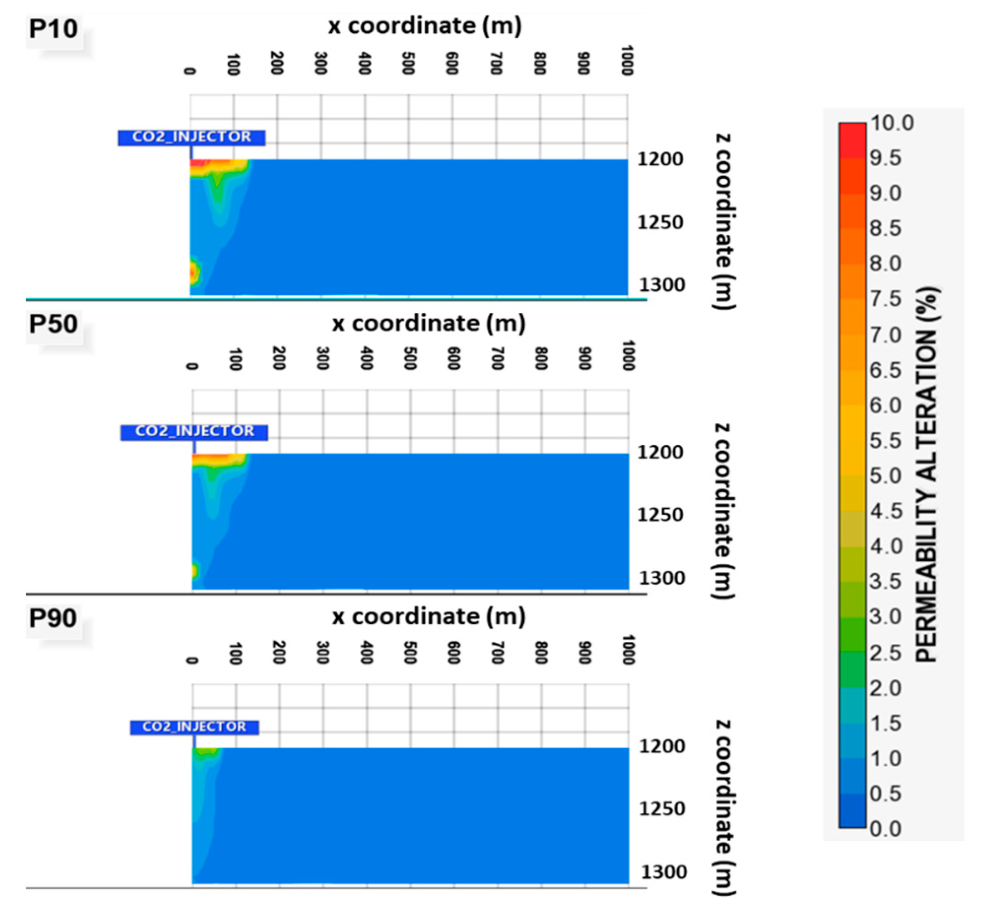
  • Permeability alteration due to mineral precipitation or dissolution was computed by applying the Kozeny–Carman equation with an exponent value of 3, as Zeidouni et al. [51] recommended:
k k = k n / r f
where
r f = r f n φ n φ k 3 1 φ k 1 φ n 2
where the resistance factor rf is modeled by the Kozeny–Carman equation or the power–law relationship, kn and kk refer to permeability at previous (n) and current (k) timesteps, respectively. The porosity, φ, in (16) is calculated as follows:
φ = 1 + c f p p * φ * j = 1 n N j ρ m , j N j 0 ρ m , j
where φ* is the reference porosity without mineral precipitation/dissolution, Nj is the total moles of mineral j per bulk volume at the current time, N j 0   is the total moles of mineral j per bulk volume at time 0, ρm,j is the mineral molar density, cf is the rock compressibility, and p* is the reference pressure.

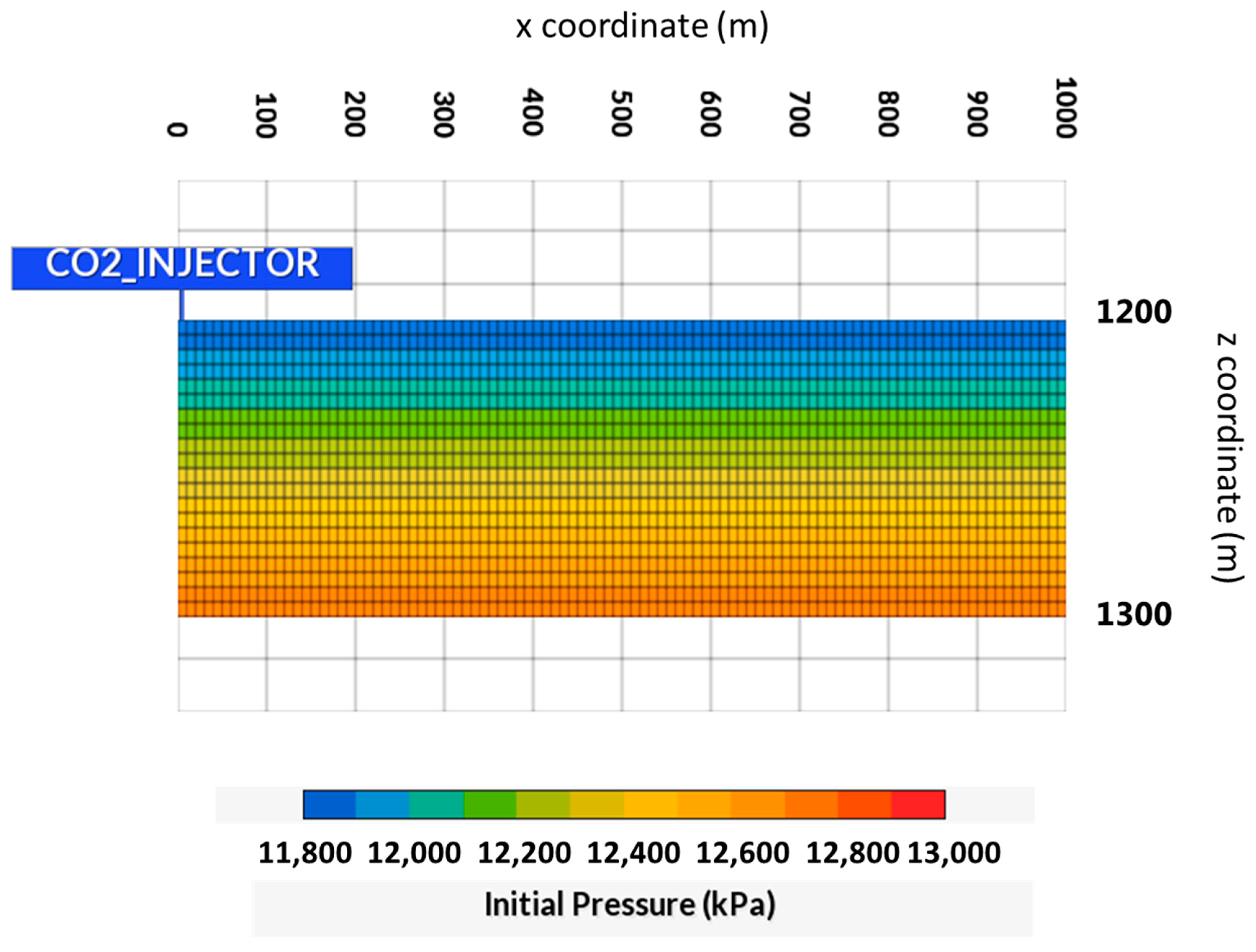
2.2. Geological Model

A synthetic 2D model of a saline aquifer was constructed, where the petrophysical properties were assumed to be homogeneous. This model was used to assess methodologies for integrating geochemical reactions and to specifically emphasize the impact of geochemistry, excluding the influence of geological heterogeneity. The model contains a vertical injector perforated in the last three bottom layers, injecting 0.5 metric tonne/day of CO2 over five years (1% of pore volume injected). Figure 1 shows the model size, discretized in 100 × 100 × 20 gridblocks with sizes of 10 m × 10 m × 5 m. The model discretization has been previously evaluated [22,32,52] and found to be suitable for representing reactive transport.
Regarding volumetric fraction, the mineralogy in this study consists of the following main primary minerals [53], which are considered relevant for the reactions and are included in the geochemical model (Table 4).
The relative permeability and capillary pressure curves for CO2 and brine in carbonates were obtained from Bennion and Bachu [54]. Figure 2 shows the drainage curves used in the simulation of the aquifer.
The residual CO2 trapping due to the relative permeability hysteresis with the saturation changes was modeled with the maximum gas trapped (Sgt) converted to the Land’s constant (C) [55] in the two-phase Carlson’s model [56], as recommended by Jarrell et al. [57], according to Equation (18):
S g t = S g   m a x 1 + C S g   m a x
where Sg max is the maximum gas saturation.
Burnside and Naylor [58] obtained Sgt distributions for CO2 and brine in sandstone, shale, and carbonates based on more than 30 published coreflood data. The mean value of Sgt = 0.25 for carbonates was assigned in this study, which is equivalent to a C = 2.4.
Other properties of this reservoir model are summarized in Table 5.

3. Results and Discussion

The objective functions (OF) that were evaluated are as follows:
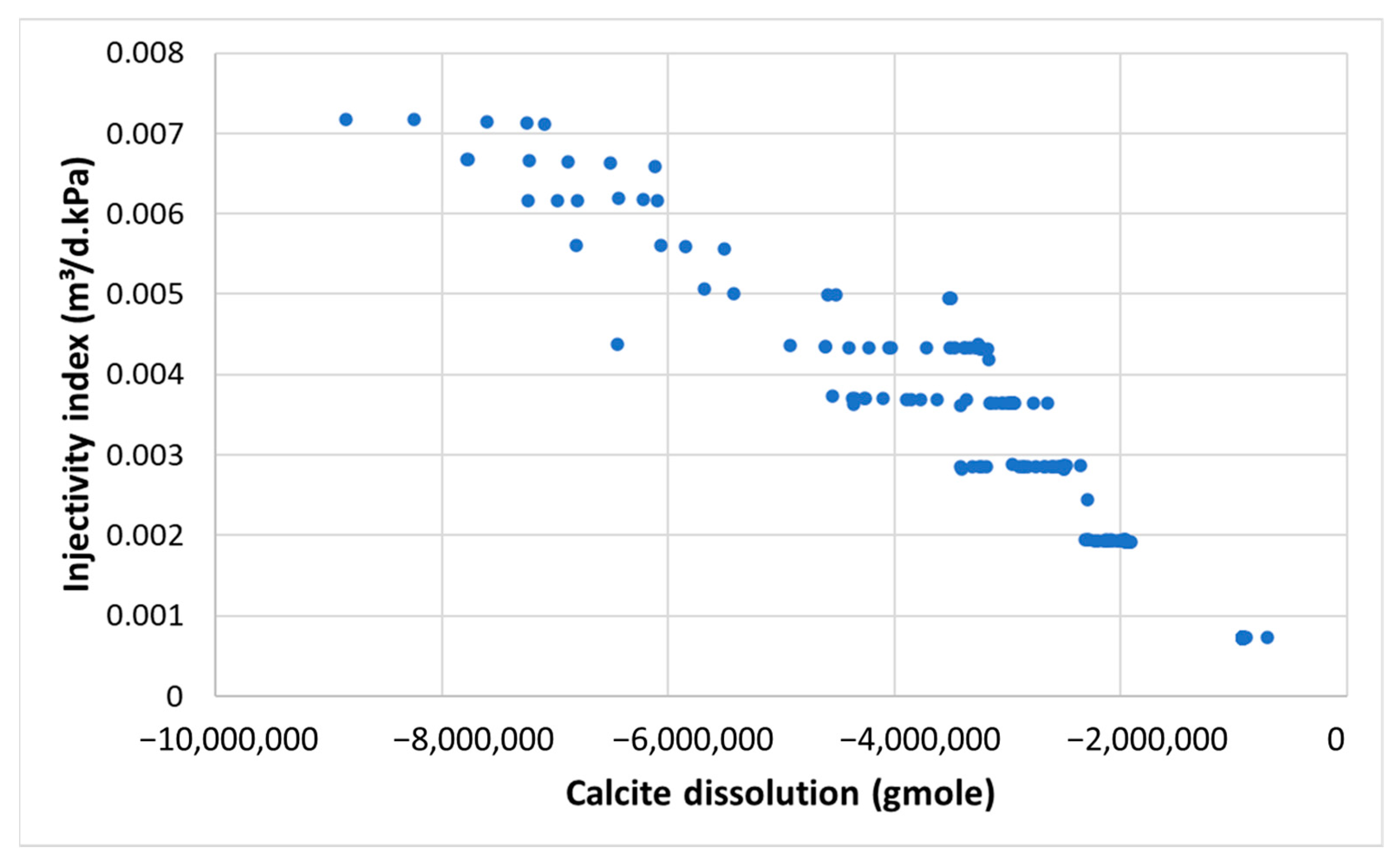
  • II: the CO2 injectivity index after five years of injection, computed according to Equation (19):
I I = q C O 2 ( p b h p ¯ a q ) ,
where II is the CO2 injectivity index, q C O 2 is the bottom-hole CO2 volumetric injection rate; pbh is the bottom-hole pressure, and p ¯ a q is the average aquifer pressure.
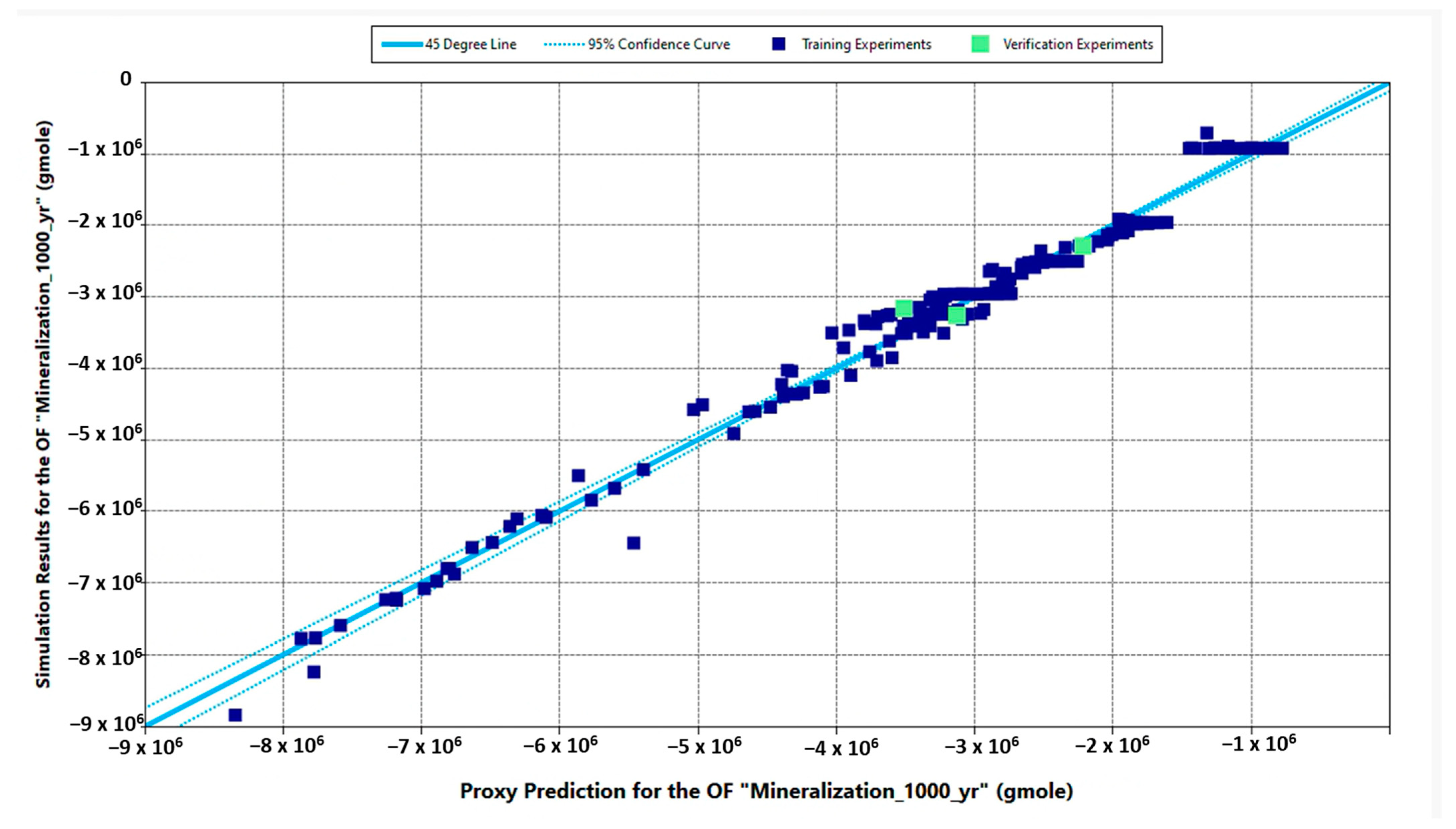
  • Mineralization_1000yr: Mineral dissolution or precipitation after 1000 years of CO2 redistribution;
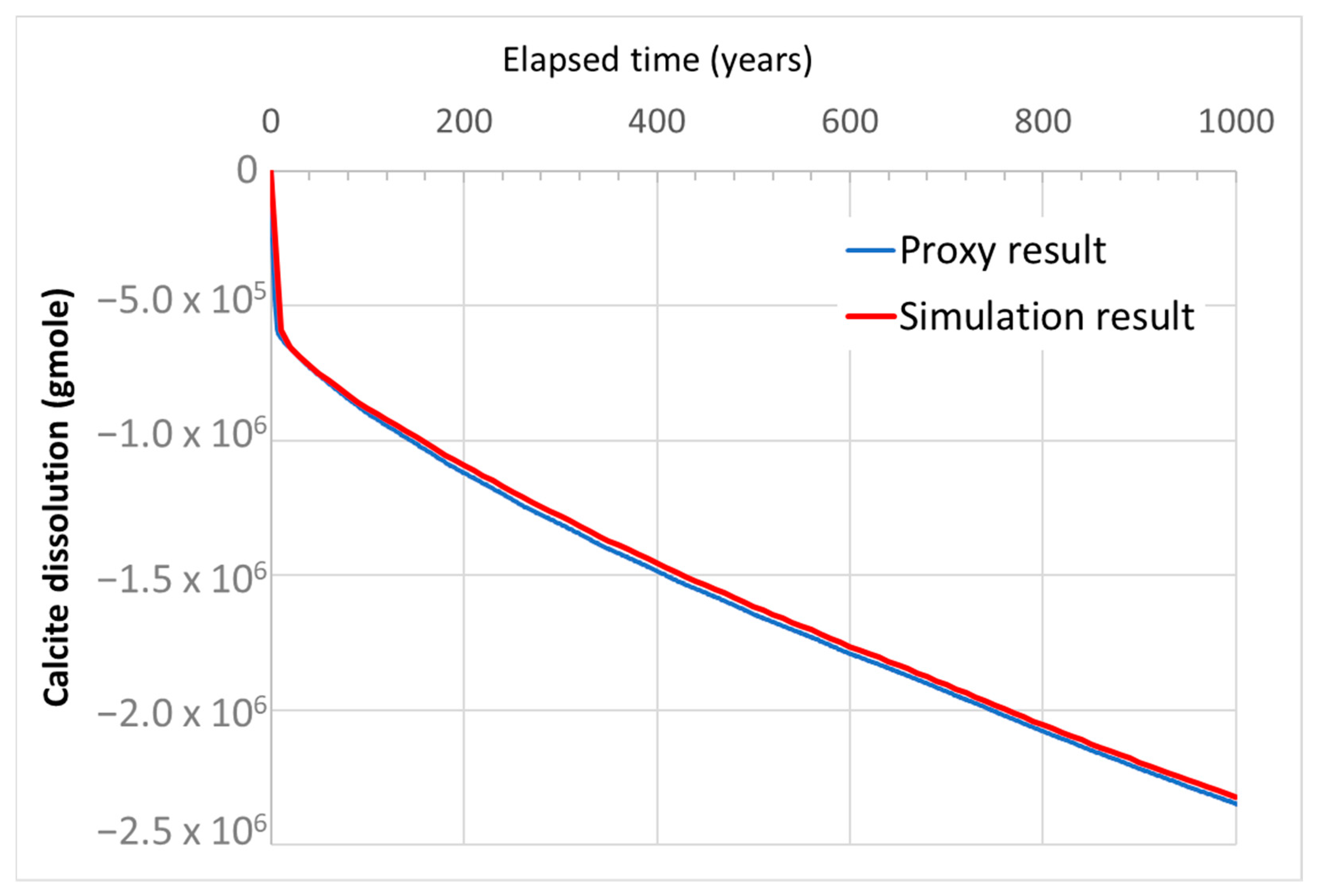
  • Calcite_1000yr: Calcite concentration change (in gmoles) after 1000 years of CO2 redistribution;
  • Dolomite_1000yr: Dolomite concentration change (in gmoles) after 1000 years of CO2 redistribution;
  • Quartz_1000yr: Quartz concentration change (in gmoles) after 1000 years of CO2 redistribution.
Table 6 summarizes the simulation results (SR) from 65,000 Monte Carlo simulations (MCS) using quadratic response surfaces (in Appendix A) as proxy models to represent the SR for each objective function (OF) in terms of the three estimates: P10, P50, and P90. In this context, the P90 represents the estimate with a 90% probability that the OF will have higher values. In other words, it signifies the lower end of the range of possible values for the OF, with only a 10% chance of the OF falling below this estimate. On the other hand, the P10 represents the upper end of the range of possible values for the OF, with only a 10% chance of the OF exceeding this estimate. The two last columns in the table display the respective R-squared (R2) coefficient, which measures the reduction in the variability of the response achieved by using the regressor variables in the model. The adjusted R2 provides an estimate of the quality of fit of a proxy model to the simulation results (600 training experiments). On the other hand, the predicted R2 is a measure of the model’s ability to accurately predict outcomes for new, unseen data (10 verification experiments), according to the representation shown in Figure 3. Overall, the results obtained from the SR and MCS analyses, along with the R2 coefficients, indicate that the proxy models built using quadratic response surfaces are reliable and provide satisfactory estimates for the objectives of this study.
The errors between the SR and MCS results were found to be lower than 5%, with an R2 higher than 80%. When considering only the P50 estimate, the prediction error decreased to less than 2%. These error levels are commonly observed in reservoir simulation applications [26,29,59]. Therefore, they were considered sufficiently accurate for this study, considering the numerous variables involved, and they will be considered for the following analysis.

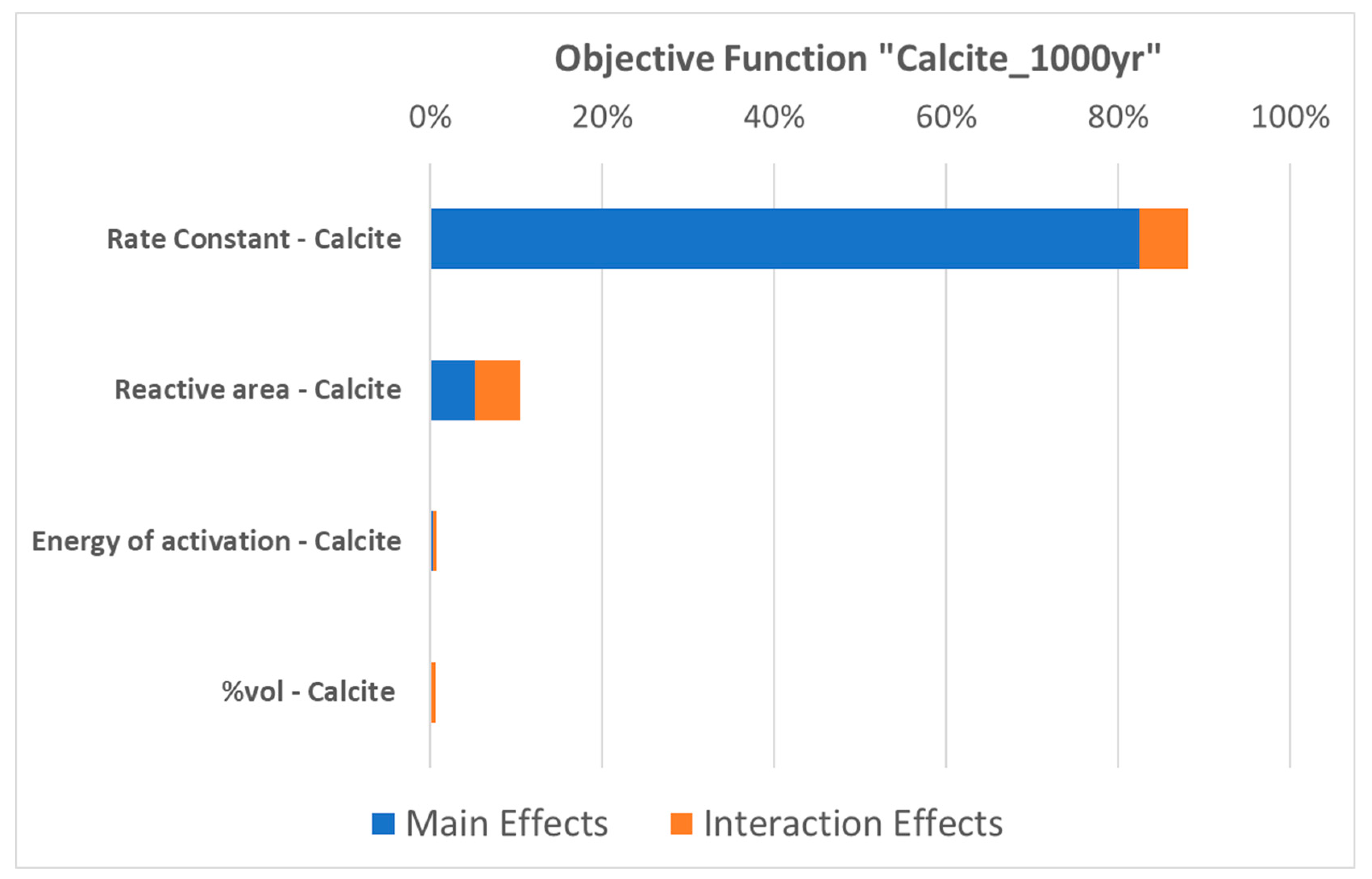
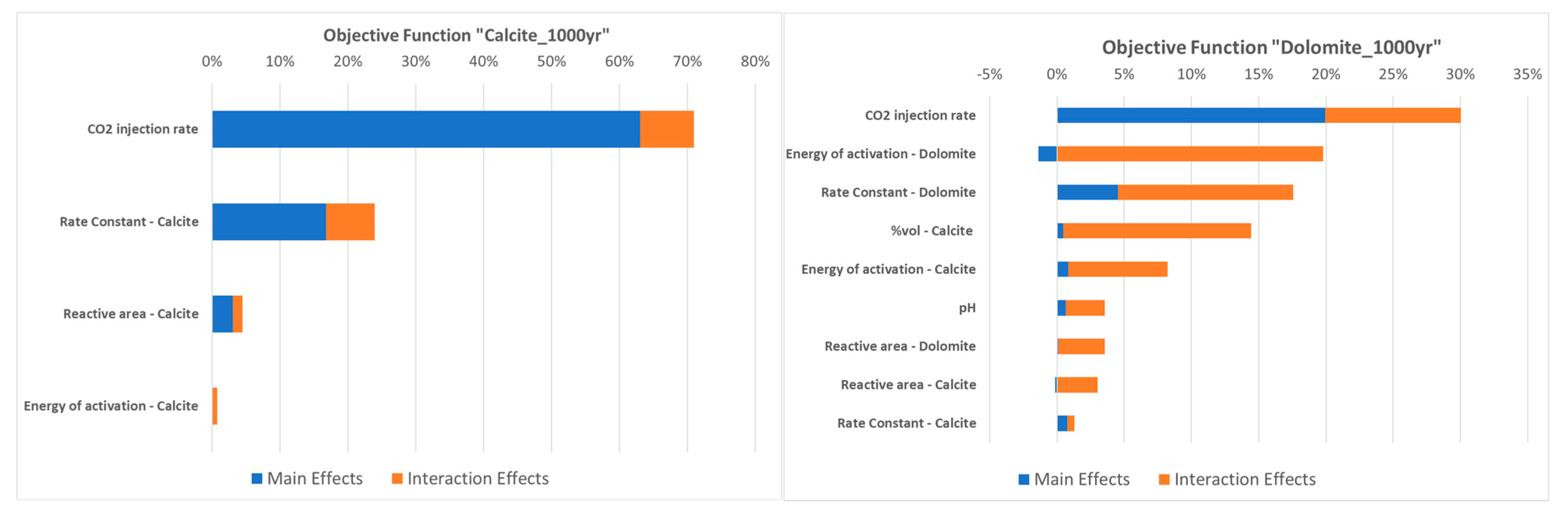
3.1. Parametric Analysis with Proxy Models for Calcite Dissolution

Calcite dissolution is the primary mineral reaction observed in this case. Consequently, the “Mineralization_1000yr” and “Calcite_1000yr” outcomes from Table 6 are practically identical. In order to better assess the impact of the volumetric percentage of calcite (%vol) on mineral dissolution, an additional parameter was introduced into the experimental design to account for different proportions of calcite, ranging from 29% to 69%. The porosity was maintained at 30%, and as the amount of calcite decreased, the amount of quartz increased at the same rate. This was conducted to simulate a transition from a carbonate-rich to a siliciclastic-rich rock, where calcite essentially acts as the rock cementation.
Figure 4 provides a summary of the sensitivity analysis using a Tornado Plot, showcasing the most influential parameter on calcite dissolution. This includes the percentage of calcite in the original rock matrix, in addition to the kinetic parameters presented in Table 3. The rate constant (k25) emerges as the most crucial parameter as it controls the reaction velocity and exhibits an explicit dependence on the energy of activation (Ea), as expressed in Equation (13) and illustrated in the interaction effect bar in Figure 4. The reactive area (A) follows as the second most influential parameter. The wide ranges of uncertainty associated with the parameters k25 and A not only exert significant control over calcite dissolution but also interact with other parameters, thereby enhancing their overall impact. The broad range of A can be attributed to its dependence on the grain size diameter of the reactive minerals present in the rock, further contributing to the variability observed. In essence, the impact of an individual parameter on the overall objective function (OF) is known as the main effect. However, interaction effects take into account combinations of model parameters that cannot be described solely by the first-order effects. This finding aligns with the results drawn by Azuddin [20] in her history-matching study involving lab experiments on carbonate cores. In order to fit the data with numerical simulations, a tuning procedure was required for the rate constant and reactive area, as demonstrated in our results, which highlight these parameters as the most influential. This type of sensitivity analysis can support history-matching studies by identifying the parameters that need to be adjusted in numerical simulations.
In this particular analysis, the percentage of calcite exhibited a minimal effect. However, as will be discussed later, the limited amount of injected CO2 is more influential in limiting the dissolution than the amount of calcite present. It explains why the difference between the P10 and P90 estimates is small for the calcite molar change.
The proxy model effectively replicates the temporal evolution of calcite dissolution. The comparison between the simulation results (in red) of a representative model for the P50 estimate and the predictions generated by the proxy model (in blue) is shown in Figure 5. In the context of reservoir simulation or modeling, representative models refer to a collection of models created to encompass the range of potential conditions or scenarios within the reservoir. These models are designed to capture various uncertainties and factors that may influence subsurface behavior, such as parameter variations or geological properties. In this particular case, the representative models correspond to the P10, P50, and P90 estimates, with the P50 estimate typically considered for project evaluation and approval.
This comparison demonstrates a notable agreement between the two sets of data, corroborating the accuracy and reliability of the proxy model. This alignment is further supported by the information presented in Table 6.
Table 7 summarizes the properties of this representative model. In this particular case, a calcite percentage of 34% was assigned, taking into account the total dissolution after 1000 years, which amounts to −2.377 × 10⁶ gmoles. It is important to note that this dissolution represents only 0.0004% of the initial calcite present in the rock matrix. This limited dissolution primarily occurs in the vicinity of the wellbore (see Section 3.3).

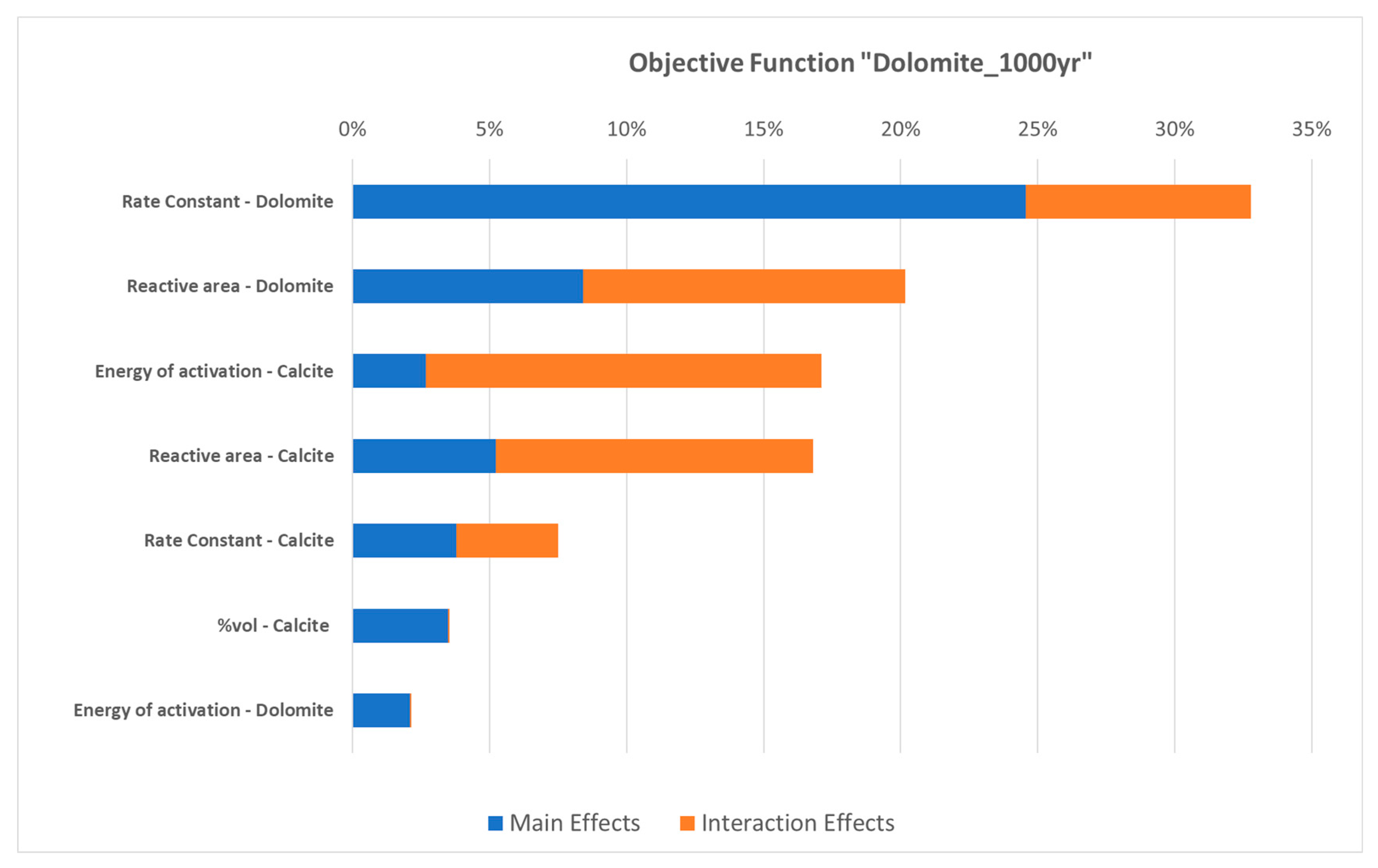
3.2. Parametric Analysis with Proxy Models for Dolomite Precipitation

In contrast to the Tornado plot for calcite dissolution (Figure 4), the dolomite Tornado plot in Figure 6 exhibits a strong interaction among the parameters, as indicated by the orange bars. This can be attributed to the fact that dolomite, in this case, is a secondary mineral formed as a result of the dissolution of calcite induced by the injection of CO2. The carbonate rock acts as a buffer, preventing a significant decrease in pH. This, coupled with the increase in HCO3 ions resulting from both the dissolved CO2 in the brine solution and calcite dissolution, leads to dolomite precipitation. As calcite dissolves, it releases Ca2+ ions into the reservoir brine, triggering dolomite precipitation and consuming Mg2+ ions from the brine solution. Importantly, the injection of CO2 induces the dolomitization process alongside calcite dissolution. This finding aligns with laboratory studies [9], which suggest that elevated temperatures exceeding 60 °C (in our case, 80 °C) initiate dolomite precipitation. It also corroborates other numerical studies [3], demonstrating the intrinsic relationship between calcite dissolution and dolomite precipitation. As a result of the strong dependencies among multiple parameters, the proxy model for dolomite demonstrates a lower quality (as indicated by the R2 value in Table 6) compared to the calcite model.
It is important to emphasize that the proxy models developed using the proposed methodology were able to capture this significant relationship between calcite dissolution and dolomite. Additionally, the models demonstrated that quartz had no impact on this dynamic due to its low reactivity, as well as the other minerals present in rock matrix with small fractions. By incorporating the relevant parameters and their interactions, our models successfully captured the complex dependencies between these two processes. This highlights the effectiveness and reliability of our approach in accurately representing the intricate interplay between calcite dissolution and dolomite precipitation.
According to Figure 6, the percentage of calcite in the rock has a positive relationship as a main effect on dolomite generation. This means that as the amount of calcite increases, more Ca2+ ions can be released into the solution, facilitating the precipitation of dolomite. This process is expected to be more efficient in alkaline pH conditions, where the CO32− ion is abundant and can support the growth of dolomite. To incorporate this aspect into the model, a new experiment was conducted, introducing the initial brine pH as a parameter with a range from 5 to 8 [60]. Figure 7 depicts the influence of pH as a parameter, displaying a strong interaction effect as it tightly stimulates dolomite generation in conjunction with the other parameters.
Unlike dolomite precipitation, the influence of pH on the calcite reaction is not as pronounced. This is because the main mechanism for calcite is dissolution, which is more likely to occur in the acidic region generated around the injector well (pH about 4), regardless of the initial pH. The acidic conditions favor the dissolution of calcite, leading to the release of calcium ions (Ca2+) into the solution. Therefore, while pH plays a significant role in dolomite precipitation, its effect on the calcite reaction is less significant. This observation is another crucial piece of evidence obtained from our study, which can be utilized to inform the design of future laboratory experiments. By identifying the key parameters that strongly influence the system, our results provide guidance on which parameters should be carefully measured and considered in experimental setups.

3.3. Thorough Proxy Analysis

The Tornado plots for calcite and dolomite, depicting the influence of various parameters after 1000 years, reveal that the rate constant emerges as the most significant kinetic parameter. This parameter holds direct control over the reaction rate, especially in the context of calcite dissolution. However, it is important to note that the rate constant also exhibits a wide range of uncertainty in open databases, as Dethlefsen et al. [12] highlighted in their analysis of batch simulation results.
Building upon the foundational research on uncertainty assessment conducted by Ates et al. [11], who suggested that geochemical reactions become more significant at higher CO2 injection rates, a new experimental design incorporated the CO2 injection rate as a variable to better understand its relevance in comparison to the rate constant. As a result, the final uncertainty analysis includes the same set of kinetic parameters for calcite, dolomite, and quartz, along with the percentage of calcite in the initial rock and the initial brine pH. Additionally, the injection rate varied over five years, ranging from 0.1 to 2.5 metric tonnes/day.
Figure 8 presents the updated Tornado plots for the objective functions (OFs) “Calcite_1000yr” and “Dolomite_1000yr”. The findings support the observations made by Ates et al. [11], as the CO2 injection rate emerges as the most influential parameter. This parameter plays a crucial role in fueling the calcite dissolution reaction, which, in turn, is closely linked to the growth of dolomite, as evidenced by the right Tornado plot in Figure 8. Consequently, a positive relationship is expected and observed between the injection rate and both calcite dissolution (with a much greater magnitude) and dolomite precipitation. These results further underscore the significance of the CO2 injection rate in driving mineral reactions and highlight its impact on the carbonate system.
The direct impact of calcite dissolution can be quantified by monitoring the evolution of injectivity, which serves as an important parameter in laboratory experiments and field-scale operations. By applying Equations (15)–(17), the rock porosity and permeability can be updated as a result of geochemical reactions, leading to an increase in the injectivity index (II). Considering the significant uncertainty associated with calcite dissolution, injectivity uncertainty is expected to also increase proportionally to the extent of calcite dissolution, particularly at higher injection rates, as illustrated in the left Tornado plot in Figure 8 and the crossplot in Figure 9.
Table 8 provides an assessment of the uncertainty level, measured by the ratio of II in the P90 estimate to that in the P10 estimate. By comparing the first experiment (Section 4), where the CO2 injection rate was fixed at 0.5 tonne/day, with the second experiment, which incorporates a broad range of CO2 injection rates as a parameter, the table highlights the uncertainty increase associated with injectivity in the second experiment, where greater amounts of CO2 are involved. This information can be valuable in field and laboratory tests, as it aids in calibrating the balance between the dissolution and precipitation of carbonate minerals, with injectivity serving as a monitoring parameter, in addition to the effluent composition.
It is important to acknowledge that precipitation reactions of other secondary minerals, such as halite scale in the dry-out zone, can occur and partially counteract the changes in porosity and permeability resulting from calcite dissolution. Although this specific effect was not evaluated in the present study, it has been extensively studied and documented in work conducted by Machado et al. [22,61].
The significant variation observed in the permeability changes among the different scenarios depicted in Figure 10 reflects the uncertainty quantified in Table 8 when the CO2 injection is a parameter. Furthermore, the primary changes observed in the model are concentrated at the top of the injection interval and in the shallowest layers. This observation raises concerns regarding the integrity of the caprock, as discussed in [62]. These changes can be attributed to the upward migration of CO2 within the reservoir, driven by its buoyancy, resulting in a localized concentration of effects near the injection zone.
The uncertainty highlighted in this analysis emphasizes the range of potential outcomes and the importance of carefully considering the uncertainties associated with alterations in injectivity induced by calcite dissolution. Understanding and monitoring these uncertainties is crucial for ensuring the long-term effectiveness and integrity of CO2 storage projects.

4. Conclusions

In conclusion, despite the use of a specific and simple geological model, the uncertainty analysis conducted in this study allows for the expansion and generalization of the main conclusions, providing valuable insights into carbonate reactions and informing future research and experimentation in this field. They are summarized as follows:
  • The workflow employed in this study successfully mapped the uncertainty associated with the amount of CO2 mineralized in carbonate rocks. This is essential for defining mitigation measures to address the risk of leakage in storage targets containing reactive minerals within their matrix;
  • Proxy models constructed using quadratic response surfaces effectively represented the objective functions used to evaluate CO2 injectivity and mineralization over extended periods of CO2 redistribution. These models performed well even with a relatively small number of runs, making them valuable decision-making tools;
  • The development of proxy models allowed for an expanded parametric analysis and facilitated the examination of the relationships among kinetic parameters and other key properties, such as the CO2 injection rate, brine pH, and the initial percentage of calcite in the rock matrix. The findings highlight the significance of calcite dissolution as the primary mechanism of mineralization and the interplay between pH, available CO2, and dolomite and calcite kinetics for the formation of dolomite as a secondary mineral;
  • The parametric assessment revealed that the rate constant emerges as the most significant kinetic parameter. This parameter holds direct control over the reaction rate, especially in the context of calcite dissolution. Therefore, the uncertainty on this parameter underscores the need for further research and data collection to improve our understanding and its characterization, as highlighted in our results;
  • Both pH and the initial concentration of calcite exert significant control on dolomite precipitation, while the CO2 injection rate affects both calcite dissolution and dolomite generation. No changes in quartz content were observed in the conducted numerical experiments;
  • The CO2 injectivity index has demonstrated its capability to reflect the uncertainty associated with carbonate mineral reactions. Therefore, tracking the injectivity index from field or lab tests provides a practical means of monitoring and quantifying the levels of uncertainty involved.
These conclusions provide valuable support for the design of laboratory experiments, specifically regarding the measurement of geochemical reactions in corefloods. Parameters such as calcite amount, initial brine pH, and injection rate can be carefully controlled and varied in these experiments to enhance our understanding of carbonate mineral reactions.
Furthermore, to improve the accuracy of existing databases for characterizing mineral reactions induced by CO2 injection in carbonate rocks, it is highly beneficial to further explore key parameters such as the rate constant and reactive area of the involved minerals. This can be achieved through the history matching of laboratory experiments, where these parameters are refined and adjusted to better align with observed data. By iteratively refining these parameters during the history-matching process, the precision and reliability of the current databases can be significantly improved. This, in turn, enhances our ability to accurately characterize and predict mineral reactions in carbonate rocks induced by CO2 injection.
The findings yield valuable insights into the feasibility of CCS in carbonate saline aquifers by modeling the geochemical reactions and mapping the associated risks. This information is crucial for developing and implementing effective CCS strategies in geological formations that are not typically prioritized for carbon storage, such as carbonate rocks.

Author Contributions

Conceptualization, M.V.B.M. and A.K.; methodology, M.V.B.M. and A.K.; software, M.V.B.M.; validation, M.V.B.M., A.K. and M.D.; formal analysis, M.V.B.M.; investigation, M.V.B.M. and A.K.; resources, M.V.B.M. and M.D.; data curation, M.V.B.M. and M.D.; writing—original draft preparation, M.V.B.M.; writing—review and editing, A.K. and M.D.; visualization, M.V.B.M.; supervision, M.D.; project administration, A.K.; funding acquisition, A.K. All authors have read and agreed to the published version of the manuscript.

Funding

This research was partially funded by the U.S. Department of Energy Office of Science, Basic Energy Sciences’ Geoscience program under Award Number DE-SC0024642 (Aaditya Khanal and Mojdeh Delshad) and the National Science Foundation Award under CBET-2245484 (Aaditya Khanal). Any opinions, findings, conclusions or recommendations expressed in this material are those of the author(s) and do not necessarily reflect the views of the funding agencies.

Institutional Review Board Statement

Not applicable.

Informed Consent Statement

Not applicable.

Data Availability Statement

The data and model details used in this study are provided within the article.

Acknowledgments

The authors would also like to acknowledge Karim Salaheddine for his valuable contributions in collecting geochemical data and engaging in insightful discussions.

Conflicts of Interest

The authors declare no conflicts of interest. Author Marcos Vitor Barbosa Machado was employed by the company Petrobras The remaining authors declare that the research was conducted in the absence of any commercial or financial relationships that could be construed as a potential conflict of interest.

Nomenclature

Areactive surface area, m2/m3;
aiactivity of component I, dimensionless;
Eaactivation energy, J/mol;
H i Henry’s constant at current pressure (p) and temperature (T), dimensionless;
H i * Henry’s constant at reference pressure (p*) and temperature (T), dimensionless;
IICO2 injectivity index, m3/d-kPa;
Krock permeability, mD;
Keqchemical equilibrium constant, dimensionless;
krate constant, mol/m2s;
nctnumber of reactant components, dimensionless;
Pbhbottom-hole pressure, kPa;
p ¯ a q average aquifer pressure, kPa;
Qactivity product, dimensionless;
q C O 2 bottom-hole CO2 volumetric injection rate, m3/d;
rreaction rate, mol/kg.s;
Runiversal gas constant, 8.314 kPa·L/mol·K;
Sgtresidual gas saturation due to hysteresis, dimensionless;
Sg maxmaximum gas saturation, dimensionless;
Slcurrent fluid saturation, dimensionless;
Ttemperature, K;
v i ¯ partial molar volume at infinite dilution, L/mol;
%volvolumetric percentage of calcite, %;
wiactivity power, dimensionless.
Greek symbols
φrock porosity, dimensionless;
ξ ,   ζ parameters from TST model, dimensionless.
Subscripts
lfluid (w—water or CO2);
icomponent.
Acronyms
CCSCarbon Capture and Storage;
IAPion activity product;
MCSMonte Carlo simulation;
OFobjective function;
SRsimulation results;
TSTTransition State Theory.

Appendix A

Table A1 presents the proxy models for the OFs outlined in Table 6.
Table A1. Response surfaces for the four objective functions evaluated.
Objective FunctionResponse Surface
II
(m3/d.kPa)
II = 0.00256546 − 1.59671 × 10⁻⁶ × log10(Acalcite) + 5.30525 × 10⁻⁷ × log10(Adolomite) + 7.61884 × 10⁻¹¹ × log10(Aquartz) − 6.03749 × 10⁻¹¹ × Ea calcite − 1.09612 × 10⁻¹⁰ × Ea dolomite + 2.34945 × 10⁻¹¹ × Ea quartz + 4.76277 × 10⁻⁷ × k25 calcite + 5.92785 × 10⁻⁷ × k25 dolomite + 1.99527 × 10⁻⁷ × k25 quartz − 1.01812 × 10⁻⁵ × %volcalcite + 1.05155 × 10⁻¹⁷ × log10(Acalcite) × log10(Adolomite) + 1.32612 × 10⁻¹¹ × log10(Acalcite) × Ea dolomite − 3.73041 × 10⁻⁷ × log10(Acalcite) × k25 calcite − 2.09195 × 10⁻⁷ × log10(Adolomite) × log10(Adolomite) − 1.1835 × 10⁻¹¹ × log10(Adolomite) × Ea dolomite − 7.6864 × 10⁻⁸ × log10(Adolomite) × k25 quartz − 4.15169 × 10⁻¹⁴ × log10(Aquartz) × log10(Aquartz) − 9.97032 × 10⁻¹⁵ × log10(Aquartz) × Ea calcite − 1.96966 × 10⁻¹¹ × log10(Aquartzk25 calcite − 3.8904 × 10⁻¹¹ × log10(Aquartz) × k25 dolomite +5.64032 × 10⁻¹⁰ × log10(Aquartz) × %volcalcite +8.70077 × 10⁻¹⁶ × Ea calcite × Ea dolomite +9.16404 × 10⁻¹⁶ × Ea calcite × Ea quartz − 1.31598 × 10⁻¹¹ × Ea calcite × k25 calcite − 7.78977 × 10⁻¹² × Ea calcite × k25 dolomite +6.09312 × 10⁻¹² × Ea calcite × k25 quartz − 6.75202 × 10⁻¹² × Ea dolomite × k25 quartz +3.8721 × 10⁻¹² × Ea quartz × k25 calcite +5.05183 × 10⁻¹² × Ea quartz × k25 quartz +6.21285 × 10⁻¹¹ × Ea quartz × %volcalcite − 1.72748 × 10⁻⁷ × k25 calcite × k25 calcite − 1.33993 × 10⁻⁸ × k25 calcite × k25 dolomite +2.77643 × 10⁻⁸ × k25 calcite × k25 quartz +4.7949 × 10⁻⁷ × k25 calcite × %volcalcite +1.91192 × 10⁻⁸ × k25 dolomite × k25 dolomite − 2.7037 × 10⁻⁷ × k25 quartz × %volcalcite
“Mineralization_1000yr”
(gmole)
Mineralization_1000yr = − 2.56092 × 10⁶ − 78810.2 × log10(Acalcite) + 81857.1 × log10(Adolomite) + 5.47112 × log10(Aquartz) − 6.86334 × Ea calcite + 6.65629 × Ea dolomite–0.22563 × Ea quartz − 91559.1 × k25 calcite + 8129.79 × k25 dolomite + 6397.31 × k25 quartz + 81749.7 × %volcalcite − 19001.2 × log10(Acalcite) × log10(Acalcite) − 7830.34 × log10(Acalcite) × log10(Adolomite) − 0.804756 × log10(Acalcite) × Ea calcite − 0.836512 × log10(Acalcite) × Ea dolomite +0.224363 × log10(Acalcite) × Ea quartz − 32959.3 × log10(Acalcite) × k25 calcite − 4158.36 × log10(Acalcite) × k25 quartz − 29206.4 × log10(Acalcite) × %volcalcite + 1868.44 × log10(Adolomite) × k25 dolomite + 3510.25 × log10(Adolomite) × k25 quartz + 0.000293547 × log10(Aquartz) × Ea calcite − 0.000200297 × log10(Aquartz) × Ea dolomite + 0.730634 × log10(Aquartz) × k25 calcite + 1.11503 × log10(Aquartz) × k25 dolomite − 1.06921 × log10(Aquartz) × k25 quartz − 17.5626 × log10(Aquartz) × %volcalcite − 4.29981 × 10⁻⁵ × Ea calcite × Ea dolomite − 2.42536 × 10⁻⁵ × Ea calcite × Ea quartz − 0.65069 × Ea calcite × k25 calcite − 0.411025 × Ea calcite × k25 quartz + 2.95256 × Ea calcite × %volcalcite − 5.45726 × 10⁻⁵ × Ea dolomite × Ea dolomite− 0.109345 × Ea dolomite × k25 calcite − 0.162247 × Ea dolomite × k25 dolomite + 3.78857 × Ea dolomite × %volcalcite− 0.159753 × Ea quartz × k25 calcite − 1.20835 × Ea quartz × %volcalcite − 18328.2 × k25 calcite × k25 calcite +1183.54 × k25 calcite × k25 dolomite − 979.136 × k25 calcite × k25 quartz − 16958.1 × k25 calcite × %volcalcite − 12464.1 × k25 dolomite × %volcalcite + 16942.6 × k25 quartz × %volcalcite
“Calcite_1000yr”
(gmole)
Calcite_1000yr = − 2.56106 × 10⁶ − 78790.8 × log10(Acalcite) + 81840.5 × log10(Adolomite) + 5.46552 × log10(Aquartz) − 6.86332 × Ea calcite + 6.65732 × Ea dolomite − 0.225763 × Ea quartz − 91561.3 × k25 calcite + 8129.3 × k25 dolomite + 6395.27 × k25 quartz + 81740.7 × %volcalcite − 19002.2 × log10(Acalcite) × log10(Acalcite) − 7829.64 × log10(Acalcite) × log10(Adolomite) − 0.80482 × log10(Acalcite) × Ea calcite − 0.836622 × log10(Acalcite) × Ea dolomite +0.224371 × log10(Acalcite) × Ea quartz − 32959.4 × log10(Acalcite) × k25 calcite − 4157.52 × log10(Acalcite) × k25 quartz − 29200.9× log10(Acalcite) × %volcalcite + 1866.9 × log10(Adolomite) × k25 dolomite + 3510.1 × log10(Adolomite) × k25 quartz + 0.000293499 × log10(Aquartz) × Ea calcite − 0.000200249 × log10(Aquartz) × Ea dolomite + 0.730337 × log10(Aquartz) × k25 calcite + 1.11491 × log10(Aquartz) × k25 dolomite − 1.06935 × log10(Aquartz) × k25 quartz − 17.561 × log10(Aquartz) × %volcalcite − 4.29945 × 10⁻⁵ × Ea calcite × Ea dolomite − 2.4253 × 10⁻⁵ × Ea calcite × Ea quartz − 0.650722 × Ea calcite × k25 calcite − 0.411022 × Ea calcite × k25 quartz + 2.95273 × Ea calcite × %volcalcite − 5.45765 × 10⁻⁵ × Ea dolomite × Ea dolomite − 0.109326 × Ea dolomite × k25 calcite − 0.16221 × Ea dolomite × k25 dolomite + 3.78793 × Ea dolomite × %volcalcite − 0.159745 × Ea quartz × k25 calcite − 1.20803 × Ea quartz × %volcalcite − 18328.2 × k25 calcite × k25 calcite +1183.34 × k25 calcite × k25 dolomite − 979.243 × k25 calcite × k25 quartz − 16957.4 × k25 calcite × %volcalcite − 12461 × k25 dolomite × %volcalcite + 16942.1 × k25 quartz × %volcalcite
“Dolomite_1000yr”
(gmole)
Dolomite_1000yr = 41.2594 − 9.40417 × log10(Acalcite) + 8.53233 × log10(Adolomite) + 0.0024599× log10(Aquartz) − 0.000209106 × Ea calcite +2.73214 × 10⁻⁵ × Ea dolomite + 0.000210498 × Ea quartz + 0.580279 × k25 calcite + 5.29976 × k25 dolomite − 2.81628 × k25 quartz + 10.4168 × %volcalcite +0.422753 × log10(Acalcite) × log10(Acalcite) − 0.000383179 × log10(Acalcite) × log10(Aquartz) +5.71373 × 10⁻⁵ × log10(Acalcite) × Ea calcite + 4.98471 × 10⁻⁵ × log10(Acalcite) × Ea dolomite + 0.111153 × log10(Acalcite) × k25 calcite − 0.453818 × log10(Acalcite) × k25 quartz − 2.45546 × log10(Acalcite) × %volcalcite + 0.903354 × log10(Adolomite) × log10(Adolomite) − 5.24884 × 10⁻⁵ × log10(Adolomite) × Ea dolomite − 3.46002 × 10⁻⁵ × log10(Adolomite) × Ea quartz + 0.18789 × log10(Adolomite) × k25 calcite + 0.816175 × log10(Adolomite) × k25 dolomite−2.43872 × log10(Adolomite) × %volcalcite +1.84261 × 10⁻⁸ × log10(Aquartz) × Ea calcite − 2.77418 × 10⁻⁸ × log10(Aquartz) × Ea dolomite +1.12908 × 10⁻⁸ × log10(Aquartz) × Ea quartz + 0.000120776 × log10(Aquartz) × k25 calcite + 6.67237 × 10⁻⁵ × log10(Aquartz) × k25 dolomite − 0.000946578 × log10(Aquartz) × %volcalcite +1.49461 × 10⁻⁵ × Ea calcite × k25 calcite − 2.05779 × 10⁻⁹ × Ea dolomite × Ea quartz − 1.21957 × 10⁻⁵ × Ea dolomite × k25 calcite − 1.9527 × 10⁻⁵ × Ea dolomite × k25 dolomite + 0.000290175 × Ea dolomite × %volcalcite − 4.67258 ×10⁻⁶ × Ea quartz × k25 calcite − 0.000187437 × Ea quartz × %volcalcite + 0.123451 × k25 calcite × k25 dolomite + 0.0592084 × k25 calcite × k25 quartz +0.319923× k25 dolomite × k25 dolomite +0.0799563× k25 dolomite × k25 quartz − 1.76213 × k25 dolomite × %volcalcite–0.204805 × k25 quartz × k25 quartz
“Quartz_1000yr”It was not possible to calibrate a response surface due to the absence of variation in quartz content.

References

  1. Dai, Z.; Xu, L.; Xiao, T.; McPherson, B.; Zhang, X.; Zheng, L.; Dong, S.; Yang, Z.; Soltanian, M.R.; Yang, C.; et al. Reactive Chemical Transport Simulations of Geologic Carbon Sequestration: Methods and Applications. Earth-Sci. Rev. 2020, 208, 103265. [Google Scholar] [CrossRef]
  2. Yamasaki, A. An Overview of CO2 Mitigation Options for Global Warming-Emphasizing CO2 Sequestration Options. J. Chem. Eng. Jpn. (JCEJ) 2003, 36, 361–375. [Google Scholar] [CrossRef]
  3. Han, W.S.; McPherson, B.J.; Lichtner, P.C.; Wang, F.P. Evaluation of Trapping Mechanisms in Geologic CO2 Sequestration: Case Study of SACROC Northern Platform, a 35-Year CO2 Injection Site. Am. J. Sci. 2010, 310, 282–324. [Google Scholar] [CrossRef]
  4. Jun, Y.-S.; Giammar, D.E.; Werth, C.J. Impacts of Geochemical Reactions on Geologic Carbon Sequestration. Environ. Sci. Technol. 2013, 47, 3–8. [Google Scholar] [CrossRef]
  5. Parkhurst, D.L.; Thorstenson, D.C.; Plummer, L.N. PHREEQE: A Computer Program for Geochemical Calculations; U.S. Geological Survey: Denver, CO, USA, 1980. [Google Scholar]
  6. Allison, J.D.; Brown, D.S.; Novo-Gradac, K.J. MINTEQA2/PRODEFA2: A Geochemical Assessment Model for Environmental Systems: Version 3.0 User’s Manual; U.S. Environmental Protection Agency National Exposure Research Laboratory Ecosystems Research Division: Athens, GA, USA, 1991. [Google Scholar]
  7. Wolery, T.J. EQ3/6, a Software Package for Geochemical Modeling of Aqueous Systems: Package Overview and Installation Guide (Version 7.0); UCRL-MA-110662-Pt.1; Lawrence Livermore National Lab. (LLNL): Livermore, CA, USA, 1992; p. 138894. [Google Scholar]
  8. Parkhurst, D.L.; Appelo, C.A.J. Description of Input and Examples for PHREEQC Version 3: A Computer Program for Speciation, Batch-Reaction, One-Dimensional Transport, and Inverse Geochemical Calculations. In U.S. Geological Survey Techniques and Methods, Book 6; U.S. Geological Survey: Denver, CO, USA, 2013; p. 497. [Google Scholar]
  9. Usdowski, E. Synthesis of Dolomite and Geochemical Implications. In Dolomites; Purser, B., Tucker, M., Zenger, D., Eds.; Wiley: Hoboken, NJ, USA, 1994; ISBN 978-0-632-03787-2. [Google Scholar]
  10. Hellevang, H.; Pham, V.T.H.; Aagaard, P. Kinetic Modelling of CO2–Water–Rock Interactions. Int. J. Greenh. Gas. Control 2013, 15, 3–15. [Google Scholar] [CrossRef]
  11. Ates, H.; Gupta, A.; Chandrasekar, V.; Vaidya, R.; AlMajid, M.; Yousif, Z. Ranking of Geologic and Dynamic Model Uncertainties for Carbon Dioxide Storage in Saline Aquifers. In Proceedings of the SPE Middle East Oil and Gas Show and Conference, Manama, Bahrain, 21 February 2023; SPE: Manama, Bahrain, 2023; p. D031S110R003. [Google Scholar]
  12. Dethlefsen, F.; Haase, C.; Ebert, M.; Dahmke, A. Uncertainties of Geochemical Modeling during CO2 Sequestration Applying Batch Equilibrium Calculations. Environ. Earth Sci. 2012, 65, 1105–1117. [Google Scholar] [CrossRef]
  13. Lake, L.W.; Bryant, S.L.; Araque-Martinez, A.N. Geochemistry and Fluid Flow, 1st ed.; Developments in Geochemistry; Elsevier Science Ltd.: Amsterdam, The Netherlands; New York, NY, USA, 2002; ISBN 978-0-444-50569-9. [Google Scholar]
  14. Lasaga, A.C. Chemical Kinetics of Water-Rock Interactions. J. Geophys. Res. 1984, 89, 4009–4025. [Google Scholar] [CrossRef]
  15. Gunter, W.D.; Bachu, S.; Benson, S. The Role of Hydrogeological and Geochemical Trapping in Sedimentary Basins for Secure Geological Storage of Carbon Dioxide. Geol. Soc. 2004, 233, 129–145. [Google Scholar] [CrossRef]
  16. Xu, T.; Yue, G.; Wang, F.; Liu, N. Using Natural CO2 Reservoir to Constrain Geochemical Models for CO2 Geological Sequestration. Appl. Geochem. 2014, 43, 22–34. [Google Scholar] [CrossRef]
  17. Bolourinejad, P.; Shoeibi Omrani, P.; Herber, R. Effect of Reactive Surface Area of Minerals on Mineralization and Carbon Dioxide Trapping in a Depleted Gas Reservoir. Int. J. Greenh. Gas Control 2014, 21, 11–22. [Google Scholar] [CrossRef]
  18. Jaafar Azuddin, F.; Azahree, A.I. Reservoir Simulation Study for CO2 Sequestration in a Depleted Gas Carbonate Reservoir: Impact of Mineral Dissolution and Precipitation on Petrophysical Properties. SSRN J. 2019. [Google Scholar] [CrossRef]
  19. Azuddin, F.J.; Davis, I.; Singleton, M.; Geiger, S.; Mackay, E. Modeling Mineral Reaction at Close to Equilibrium Condition During CO2 Injection for Storage in Carbonate Reservoir. In Proceedings of the EAGE 2020 Annual Conference & Exhibition Online, Online, 8–11 December 2020; European Association of Geoscientists & Engineers: Bunnik, The Netherlands, 2020; pp. 1–5. [Google Scholar]
  20. Azuddin, F.J. Numerical Simulation and Experimental Investigation of Reactive Flow in a Carbonate Reservoir; Heriot-Watt University: Edinburgh, UK, 2022. [Google Scholar]
  21. Altar, D.E.; Kaya, E.; Zarrouk, S.J.; Passarella, M.; Mountain, B.W. Reactive Transport Modelling under Supercritical Conditions. Geothermics 2023, 111, 102725. [Google Scholar] [CrossRef]
  22. Machado, M.V.B.; Delshad, M.; Sepehrnoori, K. Modeling Self-Sealing Mechanisms in Fractured Carbonates Induced by CO2 Injection in Saline Aquifers. ACS Omega 2023, 8, 48925–48937. [Google Scholar] [CrossRef]
  23. Tadjer, A.; Bratvold, R.B. Managing Uncertainty in Geological CO2 Storage Using Bayesian Evidential Learning. Energies 2021, 14, 1557. [Google Scholar] [CrossRef]
  24. Mahjour, S.K.; Faroughi, S.A. Selecting Representative Geological Realizations to Model Subsurface CO2 Storage under Uncertainty. Int. J. Greenh. Gas Control 2023, 127, 103920. [Google Scholar] [CrossRef]
  25. Khanal, A.; Shahriar, M.F. Physics-Based Proxy Modeling of CO2 Sequestration in Deep Saline Aquifers. Energies 2022, 15, 4350. [Google Scholar] [CrossRef]
  26. Machado, M.V.B.; Delshad, M.; Sepehrnoori, K. The Interplay between Experimental Data and Uncertainty Analysis in Quantifying CO2 Trapping during Geological Carbon Storage. Clean. Energy Sustain. 2024, 2, 10001. [Google Scholar] [CrossRef]
  27. Raza, Y. Uncertainty Analysis of Capacity Estimates and Leakage Potential for Geologic Storage of Carbon Dioxide in Saline Aquifers. Master’s Thesis, Massachusetts Institute of Technology, Cambridge, MA, USA, 2006. [Google Scholar]
  28. Likanapaisal, P.; Lun, L.; Krishnamurthy, P.; Kohli, K. Understanding Subsurface Uncertainty for Carbon Storage in Saline Aquifers: PVT, SCAL, and Grid-Size Sensitivity. In Proceedings of the SPE Annual Technical Conference and Exhibition, San Antonio, TX, USA, 17 October 2023; SPE: San Antonio, TX, USA, 2023; p. D021S020R002. [Google Scholar]
  29. Mckay, M.D.; Beckman, R.J.; Conover, W.J. A Comparison of Three Methods for Selecting Values of Input Variables in the Analysis of Output From a Computer Code. Technometrics 2000, 42, 55–61. [Google Scholar] [CrossRef]
  30. Ma, Y.Z. Quantitative Geosciences: Data Analytics, Geostatistics, Reservoir Characterization and Modeling; Springer International Publishing: Cham, Switzerland, 2019; ISBN 978-3-030-17859-8. [Google Scholar]
  31. Saltelli, A.; Ratto, M.; Andres, T.; Campolongo, F.; Cariboni, J.; Gatelli, D.; Saisana, M.; Tarantola, S. Global Sensitivity Analysis. The Primer, 1st ed.; Wiley: Hoboken, NJ, USA, 2007; ISBN 978-0-470-05997-5. [Google Scholar]
  32. Machado, M.V.B.; Delshad, M.; Sepehrnoori, K. A Computationally Efficient Approach to Model Reactive Transport During CO2 Storage in Naturally Fractured Saline Aquifers; SSRN: Rochester, NY, USA, 2023. [Google Scholar]
  33. Iglauer, S.; Al-Yaseri, A.Z.; Rezaee, R.; Lebedev, M. CO2 Wettability of Caprocks: Implications for Structural Storage Capacity and Containment Security. Geophys. Res. Lett. 2015, 42, 9279–9284. [Google Scholar] [CrossRef]
  34. Wang, J.; Samara, H.; Jaeger, P.; Ko, V.; Rodgers, D.; Ryan, D. Investigation for CO2 Adsorption and Wettability of Reservoir Rocks. Energy Fuels 2022, 36, 1626–1634. [Google Scholar] [CrossRef]
  35. Chen, H.; Wang, C.; Ye, M. An Uncertainty Analysis of Subsidy for Carbon Capture and Storage (CCS) Retrofitting Investment in China’s Coal Power Plants Using a Real-Options Approach. J. Clean. Prod. 2016, 137, 200–212. [Google Scholar] [CrossRef]
  36. Koelbl, B.S.; Van Den Broek, M.A.; Faaij, A.P.C.; Van Vuuren, D.P. Uncertainty in Carbon Capture and Storage (CCS) Deployment Projections: A Cross-Model Comparison Exercise. Clim. Chang. 2014, 123, 461–476. [Google Scholar] [CrossRef]
  37. Van Der Spek, M.; Fout, T.; Garcia, M.; Kuncheekanna, V.N.; Matuszewski, M.; McCoy, S.; Morgan, J.; Nazir, S.M.; Ramirez, A.; Roussanaly, S.; et al. Uncertainty Analysis in the Techno-Economic Assessment of CO2 Capture and Storage Technologies. Critical Review and Guidelines for Use. Int. J. Greenh. Gas Control 2020, 100, 103113. [Google Scholar] [CrossRef]
  38. Oda, J.; Akimoto, K. An Analysis of CCS Investment under Uncertainty. Energy Procedia 2011, 4, 1997–2004. [Google Scholar] [CrossRef]
  39. CMG. GEM Compositional & Unconventional Simulator, (Version 2023.30); Windows, CMG: Calgary, AB, Canada, 2023. [Google Scholar]
  40. Ahmadi, H.; Erfani, H.; Jamialahmadi, M.; Soulgani, B.S.; Dinarvand, N.; Sharafi, M.S. Corrigendum to “Experimental Study and Modelling on Diffusion Coefficient of CO2 in Water” Fluid Phase Equilibria 523 (2020) 112,584. Fluid. Phase Equilibria 2021, 529, 112869. [Google Scholar] [CrossRef]
  41. Li, Y.-K.; Nghiem, L.X. Phase Equilibria of Oil, Gas and Water/Brine Mixtures from a Cubic Equation of State and Henry’s Law. Can. J. Chem. Eng. 1986, 64, 486–496. [Google Scholar] [CrossRef]
  42. Bakker, R.J. Package FLUIDS 1. Computer Programs for Analysis of Fluid Inclusion Data and for Modelling Bulk Fluid Properties. Chem. Geol. 2003, 194, 3–23. [Google Scholar] [CrossRef]
  43. Bethke, C.M. Geochemical Reaction Modeling: Concepts and Applications; Oxford University Press: Oxford, UK, 1996; ISBN 978-0-19-509475-6. [Google Scholar]
  44. Pitzer, K.S. Thermodynamics of Electrolytes. I. Theoretical Basis and General Equations. J. Phys. Chem. 1973, 77, 268–277. [Google Scholar] [CrossRef]
  45. Pitzer, K.S.; Kim, J.J. Thermodynamics of Electrolytes. IV. Activity and Osmotic Coefficients for Mixed Electrolytes. J. Am. Chem. Soc. 1974, 96, 5701–5707. [Google Scholar] [CrossRef]
  46. Kharaka, Y.K.; Gunter, W.D.; Aggarwal, P.K.; Perkins, E.H.; DeBraal, J.D. SOLMINEQ.88; a Computer Program for Geochemical Modeling of Water-Rock Interactions. Department of the Interior, US Geological Survey: Washington, DC, USA, 1988. [Google Scholar]
  47. Delany, J.M.; Lundeen, S.R. The LLNL Thermochemical Data Base—Revised Data and File Format for the EQ3/6 Package; Lawrence Livermore National Lab. (LLNL): Livermore, CA, USA, 1991. [Google Scholar]
  48. Luo, S.; Xu, R.; Jiang, P. Effect of Reactive Surface Area of Minerals on Mineralization Trapping of CO2 in Saline Aquifers. Pet. Sci. 2012, 9, 400–407. [Google Scholar] [CrossRef]
  49. Xu, T.; Apps, J.A.; Pruess, K. Analysis of Mineral Trapping for CO2 Disposal in Deep Aquifers; LBNL-6992; Lawrence Berkeley National Lab. (LBNL): Berkeley, CA, USA, 2001; p. 789133. [Google Scholar]
  50. Cui, G.; Zhu, L.; Zhou, Q.; Ren, S.; Wang, J. Geochemical Reactions and Their Effect on CO2 Storage Efficiency during the Whole Process of CO2 EOR and Subsequent Storage. Int. J. Greenh. Gas Control 2021, 108, 103335. [Google Scholar] [CrossRef]
  51. Zeidouni, M.; Pooladi-Darvish, M.; Keith, D. Analytical Solution to Evaluate Salt Precipitation during CO2 Injection in Saline Aquifers. Int. J. Greenh. Gas Control 2009, 3, 600–611. [Google Scholar] [CrossRef]
  52. Machado, M.V.B.; Delshad, M.; Sepehrnoori, K. A Practical and Innovative Workflow to Support the Numerical Simulation of CO2 Storage in Large Field-Scale Models. SPE Reserv. Eval. Eng. J. 2023; in review. [Google Scholar]
  53. Xiao, Y.; Xu, T.; Pruess, K. The Effects of Gas-Fluid-Rock Interactions on CO2 Injection and Storage: Insights from Reactive Transport Modeling. Energy Procedia 2009, 1, 1783–1790. [Google Scholar] [CrossRef]
  54. Bennion, D.B.; Bachu, S. Drainage and Imbibition Relative Permeability Relationships for Supercritical CO2/Brine and H2S/Brine Systems in Intergranular Sandstone, Carbonate, Shale, and Anhydrite Rocks. SPE Reserv. Eval. Eng. 2008, 11, 487–496. [Google Scholar] [CrossRef]
  55. Land, C.S. Calculation of Imbibition Relative Permeability for Two- and Three-Phase Flow from Rock Properties. Soc. Pet. Eng. J. 1968, 8, 149–156. [Google Scholar] [CrossRef]
  56. Carlson, F.M. Simulation of Relative Permeability Hysteresis to the Nonwetting Phase; SPE: San Antonio, TX, USA, 1981; SPE-10157-MS. [Google Scholar]
  57. Jarrell, P.M. (Ed.) Practical Aspects of CO₂ Flooding; SPE Monograph Series; Henry L. Doherty Memorial Fund of AIME Society of Petroleum Engineers: Richardson, TX, USA, 2002; ISBN 978-1-55563-096-6. [Google Scholar]
  58. Burnside, N.M.; Naylor, M. Review and Implications of Relative Permeability of CO2/Brine Systems and Residual Trapping of CO2. Int. J. Greenh. Gas Control 2014, 23, 1–11. [Google Scholar] [CrossRef]
  59. Cremon, M.A.; Christie, M.A.; Gerritsen, M.G. Monte Carlo Simulation for Uncertainty Quantification in Reservoir Simulation: A Convergence Study. J. Pet. Sci. Eng. 2020, 190, 107094. [Google Scholar] [CrossRef]
  60. Liu, Q.; Maroto-Valer, M.M. Investigation of the pH Effect of a Typical Host Rock and Buffer Solution on CO2 Sequestration in Synthetic Brines. Fuel Process. Technol. 2010, 91, 1321–1329. [Google Scholar] [CrossRef]
  61. Machado, M.V.B.; Delshad, M.; Sepehrnoori, K. Injectivity Assessment for CCS Field-Scale Projects with Considerations of Salt Deposition, Mineral Dissolution, Fines Migration, Hydrate Formation, and Non-Darcy Flow. Fuel 2023, 353, 129148. [Google Scholar] [CrossRef]
  62. Machado, M.V.B.; Delshad, M.; Sepehrnoori, K. Potential Benefits of Horizontal Wells for CO2 Injection to Enhance Storage Security and Reduce Leakage Risks. Appl. Sci. 2023, 13, 12830. [Google Scholar] [CrossRef]
Figure 1. Synthetic 2D homogeneous model of a saline carbonate aquifer.
Applsci 14 01465 g001
Figure 2. Drainage CO2/brine relative permeability curves (on the left) and capillary pressure (on the right) for a carbonate rock, Bennion and Bachu [54].
Applsci 14 01465 g002
Figure 3. Proxy model prediction versus simulation results for the training (blue dots) and verification experiments (green dots).
Applsci 14 01465 g003
Figure 4. Tornado plot for the objective function “Calcite_1000 yr” generated with MCS calibrated with 600 runs.
Applsci 14 01465 g004
Figure 5. Comparison between simulation result (in red) and proxy calculation (in blue) for the temporal evolution of calcite dissolution in P50 estimate.
Applsci 14 01465 g005
Figure 6. Tornado plot for the objective function “Dolomite_1000 yr” generated with MCS calibrated with 600 runs.
Applsci 14 01465 g006
Figure 7. Tornado plot for the objective function “Dolomite_1000 yr” generated with MCS calibrated with 600 runs, including the brine pH in the experiment design.
Applsci 14 01465 g007
Figure 8. Tornado plot for the objective function “Calcite_1000yr” (on the left) and “Dolomite_1000 yr” (on the right) generated with MCS calibrated with 600 runs, including the brine pH and CO2 injection rate in the experiment design.
Applsci 14 01465 g008
Figure 9. Crossplot with the simulation results of the injectivity index after 5 years of injection and the corresponding calcite dissolution.
Applsci 14 01465 g009
Figure 10. Cross-sectional view of rock permeability gain in the representative models of P10, P50, and P90 estimates.
Applsci 14 01465 g010
Table 1. Solubility parameter at the initial conditions of the reservoir model.
PropertiesValues
Initial pressure11,800 kPa @ 1200 m
Temperature80 °C
Salinity50,000 ppm (NaCl)
H i * 5.66 × 10⁵
Table 2. Ionic composition of formation brine.
IonsConcentration (mol/kgw)
H+1.95618 × 10⁻⁶
Ca2+0.30308
Mg2+0.04185
Na+0.3234
Cl0.551
HCO30.007482
Table 3. Kinetic parameters of TST model for mineral reactions.
MineralParameterValue/RangeSource
Calcitelog10(Keq)−8.38 [5,8,46,47,48,49]
A88 to 23,000 m2/m3
log10(k25)−8.8 to −0.3 mol/m2s
Ea14,400 to 41,870 J/mol
Quartzlog10(Keq)−4.38 [5,8,46,47,49]
A2650 to 7128 m2/m3
log10(k25)−15 to −10 mol/m2s
Ea68,175 to 113,625 J/mol
Kaolinitelog10(Keq)9.80 [5,8,46,47,50]
A1760 m2/m3
log10(k25)−13 mol/m2s
Ea62,760 J/mol
Albitelog10(Keq)−19.7 [5,8,16,46,47]
A2563.38 m2/m3
log10(k25)−10.16 mol/m2s
Ea65,000 J/mol
K-feldsparlog10(Keq)−22.66[5,8,46,47,49]
A176 m2/m3
log10(k25)−12 mol/m2s
Ea67,830 J/mol
Illitelog10(Keq)−43.28 [5,8,16,46,47]
A41,888 m2/m3
log10(k25)−10.98 mol/m2s
Ea23,600 J/mol
Dolomitelog10(Keq)−16.46 [5,8,46,47,48,49]
A88 to 23,000 m2/m3
log10(k25)−9.22 to −3.19 mol/m2s
Ea36,100 to 62,760 J/mol
Sideritelog10(Keq)−10.72 [5,8,46,47]
A4046.67 m2/m3
log10(k25)−3.19 mol/m2s
Ea36,100 J/mol
Table 4. Volumetric fraction of the main primary minerals in the rock matrix.
Mineral CompositionVol. %
Quartz1.0
Kaolinite0.15
Calcite68.68
K-feldspar0.12
Albite0.05
Porosity30.0
Table 5. Summary of reservoir properties.
PropertyValue
Initial pressure11,800 kPa @ 1200 m
Temperature80 °C
Horizontal permeability100 mD
Kv/Kh ratio0.1
Porosity30%
Rock compressibility5.8 × 10−7 kPa−1
Table 6. Stochastics estimates for the objective functions using SR and MCS, associated errors, and R2 (adjusted and predicted).
Objective FunctionEstimateSR MCS Error SR and MCS (%)Adjusted R2 (%)Predicted R2 (%)
600 Runs600 Runs600 Runs600 Runs600 Runs
II
(m3/d.kPa)
P100.00255600.00255600.099.786.1
P500.00255500.00255500.0
P900.00255100.00255100.0
“Mineralization_1000yr”
(gmole)
P10−2.286 × 10⁶−2.346 × 1062.691.390.5
P50−2.377 × 10⁶−2.420 × 1061.8
P90−2.795 × 10⁶−2.892 × 1063.5
“Calcite_1000yr”
(gmole)
P10−2.286 × 10⁶−2.346 × 1062.691.390.5
P50−2.377 × 10⁶−2.420 × 1061.8
P90−2.796 × 10⁶−2.892 × 1063.4
“Dolomite_1000yr”
(gmole)
P1057.7055.24.382.080.0
P5053.4553.00.8
P9051.7150.42.5
“Quartz_1000yr”
(gmole)
P10It was not possible to calibrate a response surface because no changes were observed in relation to the initial content set for quartz throughout the simulation period.
P50
P90
Table 7. Properties of the P50 representative model.
PropertyValueUnit
Rate Constant (k25)—Calcite (log10)−8.44mol/m2s
Reactive area (A)—Calcite1202.26m2/m3
Energy of activation (Ea)—Calcite28,047J/mol
Volumetric percentage (%vol)—Calcite34%
Table 8. The ratio between P10 and P90 estimates for the CO2 injectivity index after 5 years of injection.
Numerical ExperimentP10/P90 Ratio for II
Section 3.1 and Section 3.2: Fixed CO2 injection rate of 0.5 metric tonne/day1.002
Section 3.3: CO2 injection rate as a parameter, varying from 0.1 to 2.5 metric tonnes/day3.670
Disclaimer/Publisher’s Note: The statements, opinions and data contained in all publications are solely those of the individual author(s) and contributor(s) and not of MDPI and/or the editor(s). MDPI and/or the editor(s) disclaim responsibility for any injury to people or property resulting from any ideas, methods, instructions or products referred to in the content.

