Abstract
The numerical aperture (NA) of objective lens optical (inspection) systems has been increased to achieve higher resolution. However, the depth of focus decreases with an increase in the NA, and focusing becomes difficult. Therefore, the entire optical lens in currently developed optical inspection systems must be moved to focus within the depth of focus. To achieve a high resolution, many lenses are used in optical inspection systems, increasing the size and weight of the optical systems. To address this issue, a focus control group was placed on a tube lens that could adjust its focus based on the movement of the sample in front of the objective lens. Therefore, we developed a focus range increment to focus on the range of the optical inspection system. Using objective lenses with focal lengths of 30 and 60 mm and tube lenses with a focal length of 300 mm, optical systems for 10× and 5× inspection were constructed. In the designed optical systems, the weights of the objective lenses with focal lengths of 30 and 60 mm were calculated to be approximately 844 and 570 g, respectively. These values confirm that the weight of the moving group can be reduced.
1. Introduction
Achieving a high resolution in optical inspection systems is a topic of significant research interest. To improve the resolution, the diffraction limit must be increased [1,2,3], which is proportional to the wavelength and inversely proportional to the numerical aperture (NA) [3,4,5]. Therefore, a high resolution can be achieved with shorter wavelengths such as ultraviolet rays rather than in the visible range [6,7,8]. However, generating short-wavelength light is expensive, and the samples may be damaged by high-energy light at high frequencies during manufacturing/fabrication [9,10]. According to the diffraction limit, the smallest spot in an optical system is referred to as an airy disk, as shown in Figure 1. Generally, an objective lens is not used alone in an optical inspection system but in conjunction with a tube lens to form an image on a sensor surface [11]. An airy disk is used as an indicator of resolution. Therefore, the size of the airy disk is proportional to the wavelength and inversely proportional to the NA [12].

Figure 1.
Airy disk [12].
Figure 1.
Airy disk [12].
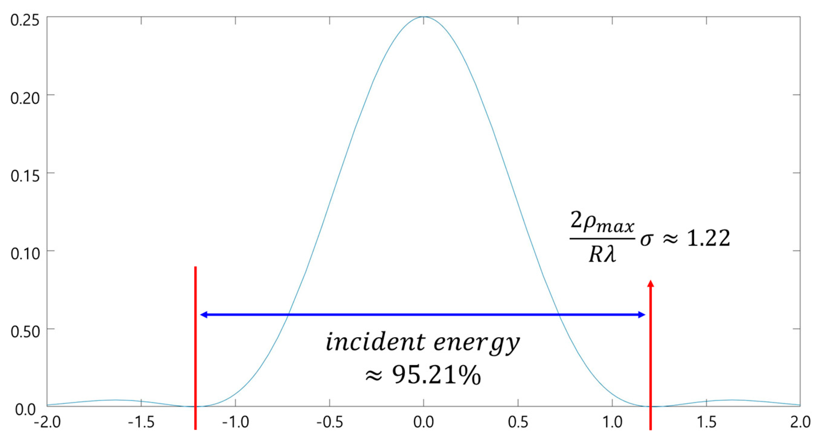
The incident energy of the zeroth-order diffraction was 95.21% when observing the intensity distribution of light passing through a circular aperture. Light passing through a circular hole diffracts and forms an interference pattern [12]. The interference pattern appeared as a repeating pattern of bright and dark shapes, with the first dark shape appearing after the first bright shape at approximately 1.22 [12]. In addition, the first point at which the zeroth-order diffraction becomes zero is approximately 1.22. Equation (1) represents the size of an airy disk, where σ indicates the airy disk, ρmax denotes the radius of the entrance pupil, R denotes the focal length, and λ represents the wavelength [12].
It can be observed that the resolution increased as the number of airy disks decreased. An optical system’s resolution is directly proportional to its NA and inversely proportional to its wavelength [13]. Studies have focused on optical systems with high NA to increase the resolution [14]. However, as the NA increases, the depth of focus of the optical system decreases, and the resolution may deteriorate as the distance between the sample and optical system changes [15]. An NA-increasing lens, also known as a plano-convex optical system, was used to increase the amount of light on the object [16,17]; however, the NA constraint on the resolution increased for the microscopy system. To achieve a high resolution, a plastic objective lens with an NA of 0.85 was proposed for use at three laser diode wavelengths [18]. A significant amount of power is required to conduct fast inspections using such systems [19]. Therefore, a fast and accurate inspection can be achieved if the sample is imaged by moving a specific lens group rather than the entire optical system. The instrument size can be minimized by reducing its motor size and weight. Additionally, heavier moving mechanisms generate more inertial forces, which can affect the results. Moreover, the equipment’s durability can also be a problem, making it difficult to control.
The amount of lens group movement must be calculated for internal autofocusing by a specific lens group at a finite object distance, including an infinite object distance. Gaussian brackets can be used for this purpose [20]. For example, an analytical calculation technique has been used for zoom lens systems [21]. The Padè approximation method was used to compute the analytical zoom locus [22].
Generally, an objective lens is not used alone in an optical inspection system but in conjunction with a tube lens to form an image on a sensor surface. Figure 2 shows a schematic of a general microscope optical system with an objective and a tube lens. In Figure 2, the objective lens magnifies the object and produces parallel light [23]. In addition, the tube lens forms an image of parallel light projected from the objective lens onto an imaging device [24].
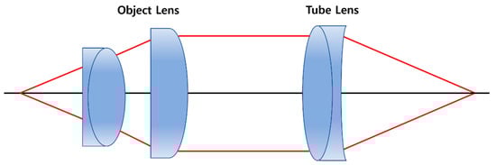
Figure 2.
Schematic of a general microscope optical system.
For magnification, the objective lens was placed close to the object, aberrations were corrected, and an image formed in the image plane using the tube lens [25]. Thus, the sample can be imaged on an imaging device that excessively widens the focus-adjustment range by moving a specific lens group within the tube lens. This focus adjustment is referred to as the internal focusing method [26]. Considering these characteristics, the magnification in a zoomed system with a Gaussian bracket remains constant, requiring the use of a telecentric optical system [27]. Therefore, we intend to design and evaluate the performance of a combined optical system in which the magnification does not change and the focus adjustment range is increased using optical design software [28]. In the design software, the zoom locus is derived using equations governing Gaussian brackets [29].
In the currently developed optical inspection system, the entire lens group must be focused, thereby compensating for the resolution based on the sample movement [30]. Therefore, current optical inspection systems are typically heavy because of the use of multiple optical lenses for aberration correction [31].
Previous studies have used telecentric optical systems for inspection applications. The structural optical design equation can aid in the design and analysis of telecentric optical systems [32]. In a double-sided telecentric optical system, a mathematical method was used to determine the design parameters using the third-order aberration method [33]. Using a Gaussian bracket and a lens module, a telecentric optical system with focus-tunable optical lenses and a moving aperture stop was analyzed [34]. Mechanical movement was reduced by combining an adaptive liquid lens with a double-sided telecentric optical system [35]. A telecentric lens module was designed for vision inspection systems with a field of view greater than 100 mm [36]. An optical design layout with three telecentric objectives for dimensional inspection systems was developed using the shadow projection method in the object space [37]. A two-dimensional telecentric system was designed by splitting the pupils and moving the principal planes using the transformed focal power [38]. An image-side telecentric anastigmatic optical system with a coaxial parent mirror was designed to obtain an ultrawide field of view [39]. A prism dispersion imaging spectrometer system was designed using imaging theory from a telecentric off-axis three-mirror imaging system [40]. A telecentric three-mirror solar simulator was proposed for large irradiation surfaces requiring high uniformity [41]. The sample arm for an optical coherent tomography system was designed [42]. The AF speed increased in the telephoto interchangeable lens [43]. To achieve high brightness in a wide-angle lens, the camera system uses two or more lens groups to accurately calculate the amount of lens movement [44]. To the best of our knowledge, this is the first optical design study for an internal focusing tube lens used in an optical inspection system. The main contributions of our study are as follows:
- The designed telecentric optical system provides a wide focus adjustment range using an internal focusing function;
- The height of the image was fixed, whereas the magnification did not change in the proposed telecentric optical system;
- As focusing is performed by moving only a specific lens group without moving the entire optical system, the inspection device can be miniaturized. Therefore, inertia control by weight is convenient, and inspection speed and accuracy are enhanced.
2. Structure and Design of the Optical System
Distortion correction using software is difficult owing to the characteristics of optical inspection systems. Therefore, the distortion control theory has been used [45,46]. Before designing the inspection optical system, we used an optical system that operated in the visible light region. Therefore, the design wavelengths were 656.27, 587.56, 546.07, 486.13, and 435.83 nm, and the center wavelength was set at 546.07 nm. The optical system was comprised of an objective and a tube lens. When the two optical systems were designed and combined, a 10× and 5× inspection optical system was configured. The specifications of the optical system were as follows: an objective lens with an NA of 0.4, a focal length of 30 mm, and an image height of 1.7 of mm; another objective lens with an NA of 0.2, a focal length of 60 mm, and an image height of 3.4 mm; and a tube lens with F/8, a focal length of 300 mm, and an image height of 17 mm. Subsequently, the objective and tube lenses were combined. The design of each objective lens begins at an infinite object point, and the optical system is configured to form an image on the image plane. By inputting the object distance at which the point moves by 50 μm and 0.36 mm based on the infinite object point at the focal lengths of 30 and 60 mm objective lenses, respectively, the design was optimized for performance close to the diffraction limit at the input object distance. The tube lens was designed to have a performance close to the diffraction limit while being able to adjust the focus for the input object’s distance based on the objective lens’s focal length of 30 mm.
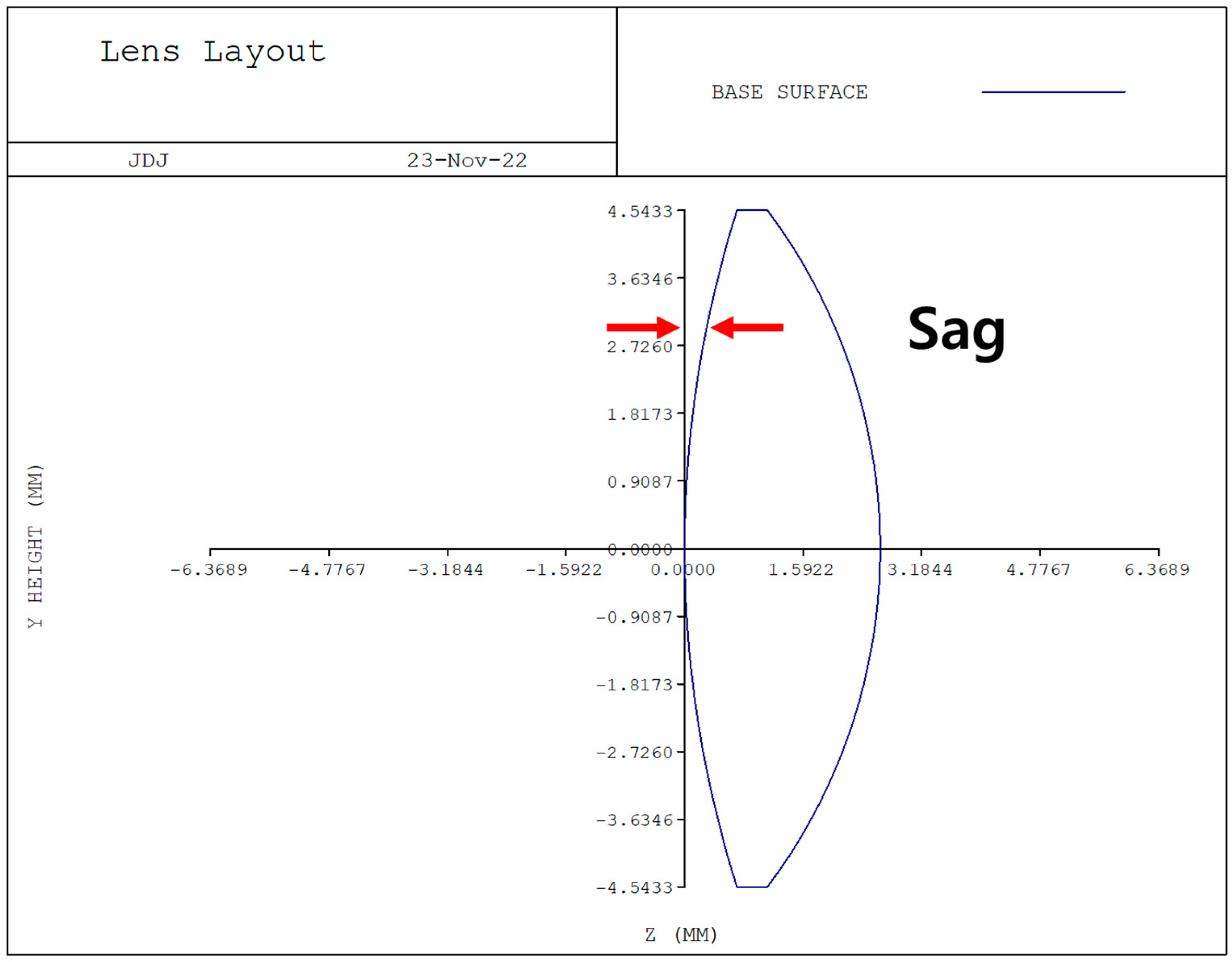
The objective and tube lenses were designed such that they acted in combination as a telecentric optical system, where the magnification did not change with the movement of the sample. Paraxial ray tracing can be used in optical system designs [47]. Paraxial ray tracing is an ideal ray-tracing method without aberrations, where the sag value owing to the curvature of the lens is approximated as zero [48]. Figure 3 shows the sag values of the lens.
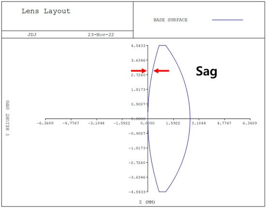
Figure 3.
Sag value of the lens.
If these sag values are minimized, paraxial ray tracing can be performed, as explained by refraction and transfer equations. Equation (2) is the refraction equation for the refraction plot of light rays at the interface between the media and the optical system. Equation (3) is the transfer equation, which describes the height of the arrival point when a ray departing from a height at a certain point enters the next boundary at a specific angle [49].
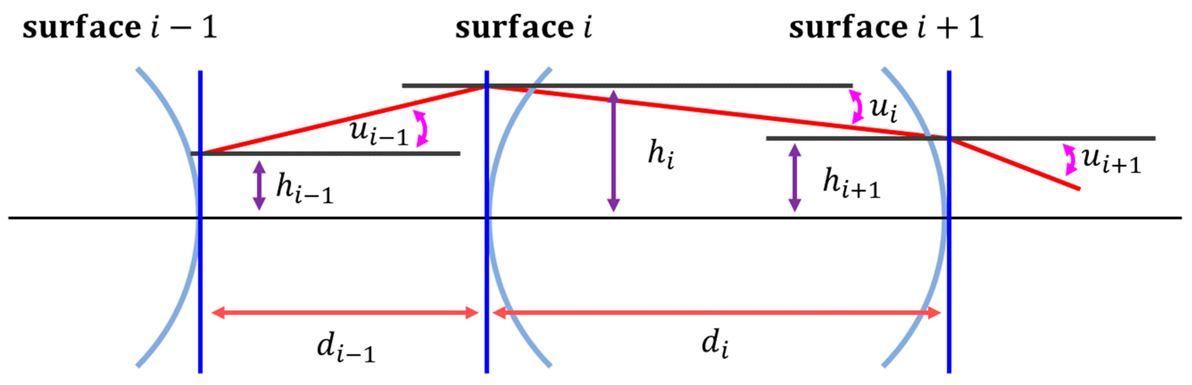
where h refers to the height of the light rays on each lens surface. A ray of light departing from one point passes at a certain angle through one lens surface and then passes through the next lens plane. Therefore, the height of the ray on the ith side is denoted as hi. k denotes the refractive power of the lens surface. The light rays are refracted based on the lens’s curvature and refractive index. The physical quantity that describes this refraction is known as the refractive power. The refractive power in the ith plane is denoted as ki. Ray tracing on multiple lens surfaces is represented by the schematic shown in Figure 4.
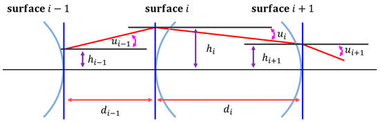
Figure 4.
Paraxial ray-tracing layout.
If paraxial ray tracing is repeated on multiple lens surfaces, the series of processes can be represented as system matrices. Equation (4) describes ray tracing from the object to the ith plane as a matrix operation [50].
Here, A, B, C, and D, comprising the system matrix, can be obtained using a Gaussian bracket operation. A Gaussian bracket operation comprising of n elements is developed, as shown in Equation (5).
If the regularity of the Gaussian bracket operation with these rules is well organized, it can be represented by the algorithm shown in Figure 5.
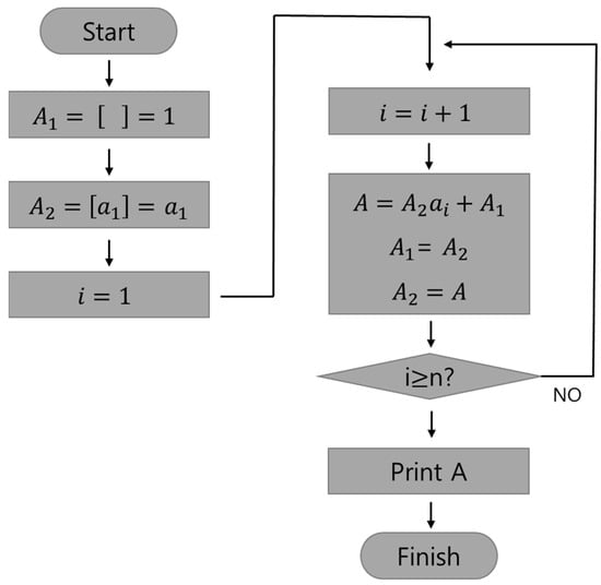
Figure 5.
Algorithm of the Gaussian bracket.
When the object distance in the optical system changes, the image distance also changes. Equation (6) shows the relationship between the object distance l and image distance variation in an optical system with focal length f [51].
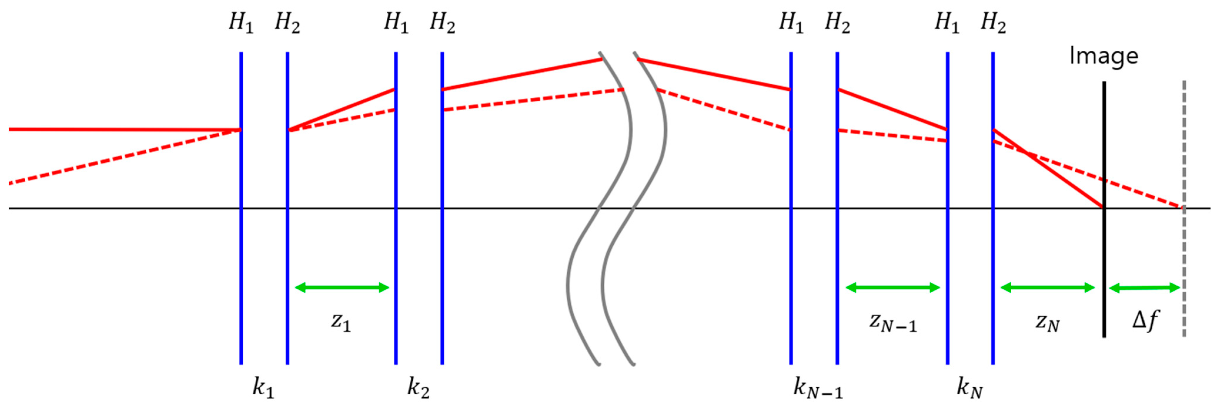
To compensate for this variation, the movement of the image plane is restricted to the movement of a specific internal lens group, as per the internal focusing method. To obtain the movement of the lens group for the image plane variance correction, the zoom equation must be solved as follows: An optical system with multiple lens groups is shown in Figure 6. Each lens group is shown in terms of the principal planes (H1, H2) and refractive power. When the refractive indices of the object and image sides of each lens group were identical, the point of intersection of the extension line of the incident light beam with an angular magnification of 1 and the optical axis was the first principal plane (H1). In addition, the intersection of the extension line of the outgoing light beam and the optical axis becomes the position of the second principal surface (H2), where zi is the distance between the principal surfaces of the ith lens group and ki is the refractive power of the ith lens. Figure 6 shows that a focus shift occurs when the object distance changes from infinity to a finite value in a zoom lens system.
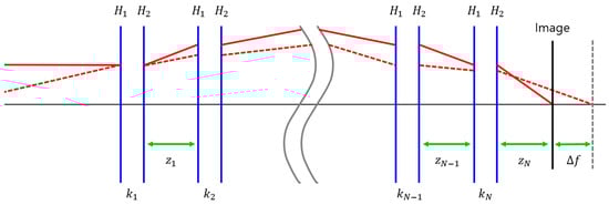
Figure 6.
Optical zoom system layout.
This optical system can be expressed using Equation (7) as follows [22]:
Equation (7) indicates that the image plane is fixed at the object distance z0 when the ith lens group of the optical system moves by δ. To find the variable δ, it should be expressed in terms of the Gaussian bracket characteristics, as shown in Equation (8). When n elements exist from a1 to an, the Gaussian brackets exhibit the same characteristics as those described in Equation (8).
Using Equation (8), Equation (7) can be expressed as Equation (9) as follows:
If α in Equation (9) is defined for δ, it is expressed in Equation (10) as follows:
Similarly, the β in Equation (9) for δ is expressed in Equation (11) as follows:
Substituting Equations (10) and (11) into Equation (9), δ variable in Equation (7) can be expressed as Equation (12) as follows:
Therefore, we can define a quadratic equation for the δ variable. A–E are defined as constants using the Gaussian bracket calculation method. The δ variable is generally selected as a smaller absolute value among real roots.
To correct this distortion, the sign of the distortion was reversed when the optical system was inverted. First, an objective lens with a focal length of 30 mm was designed, and the optical system was subsequently designed to exhibit the same distortion as that of the 30 mm objective lens. After designing the optical system, the objective lens is turned over and combined with the tube lens. When the sign of the distortion of the objective lens is reversed, the distortion of the tube lens is offset and almost eliminated. Thus, an optical system was constructed for the inspection of 10× and 5×. These magnifications were selected because 10× optical systems are used to check for foreign substances on semiconductor board surfaces, and 5× optical systems are generally used to check in detail, and are normally used in inspection optical systems.
3. Performance Analysis of the Designed Optical System
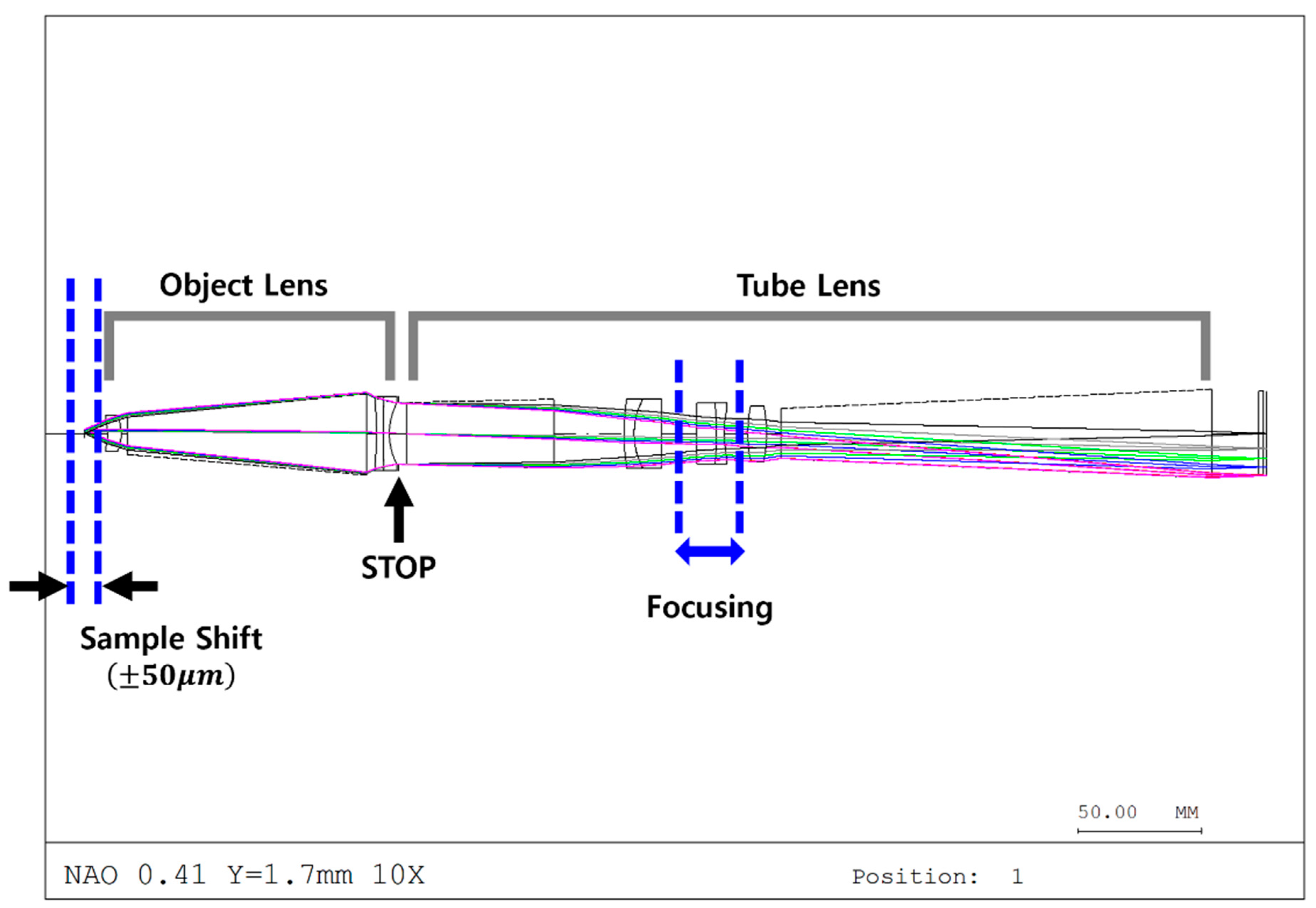
The design software used in this study was CODE V (Ver. 2023.03, Synopsis Optical System Design Inc., East Boothbay, ME, USA). An objective lens with an NA of 0.4, focal length of 30 mm, and image height of 1.7 mm; another objective lens with an NA of 0.2, focal length of 60 mm, and image height of 3.4 mm; and a tube lens with F/8, a focal length of 300 mm, and image height of 17 mm were used. It was confirmed that the optical system could adjust the focus by moving the inner lens group of the tube lens based on the sample movement and that there was no change in magnification during the focus adjustment process. Figure 7 shows the optical path diagram of the 10× optical system.

Figure 7.
Optical path diagram of the 10× optical system.
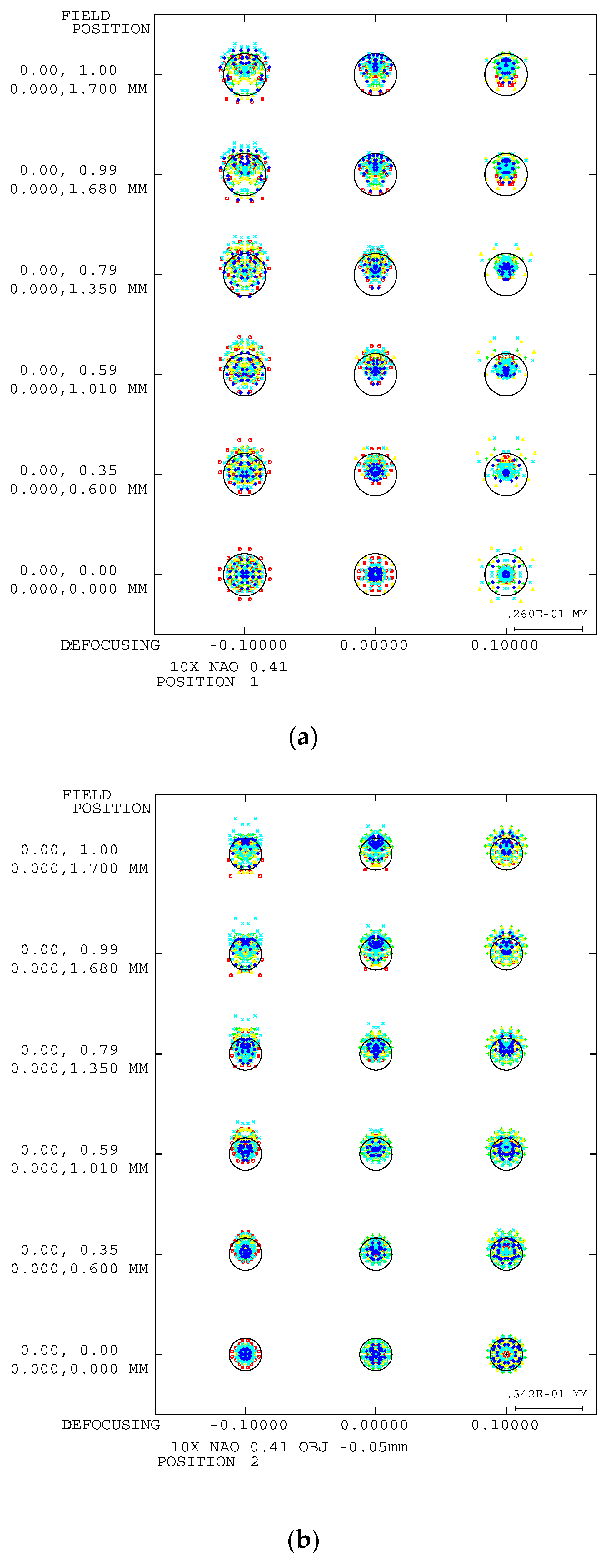
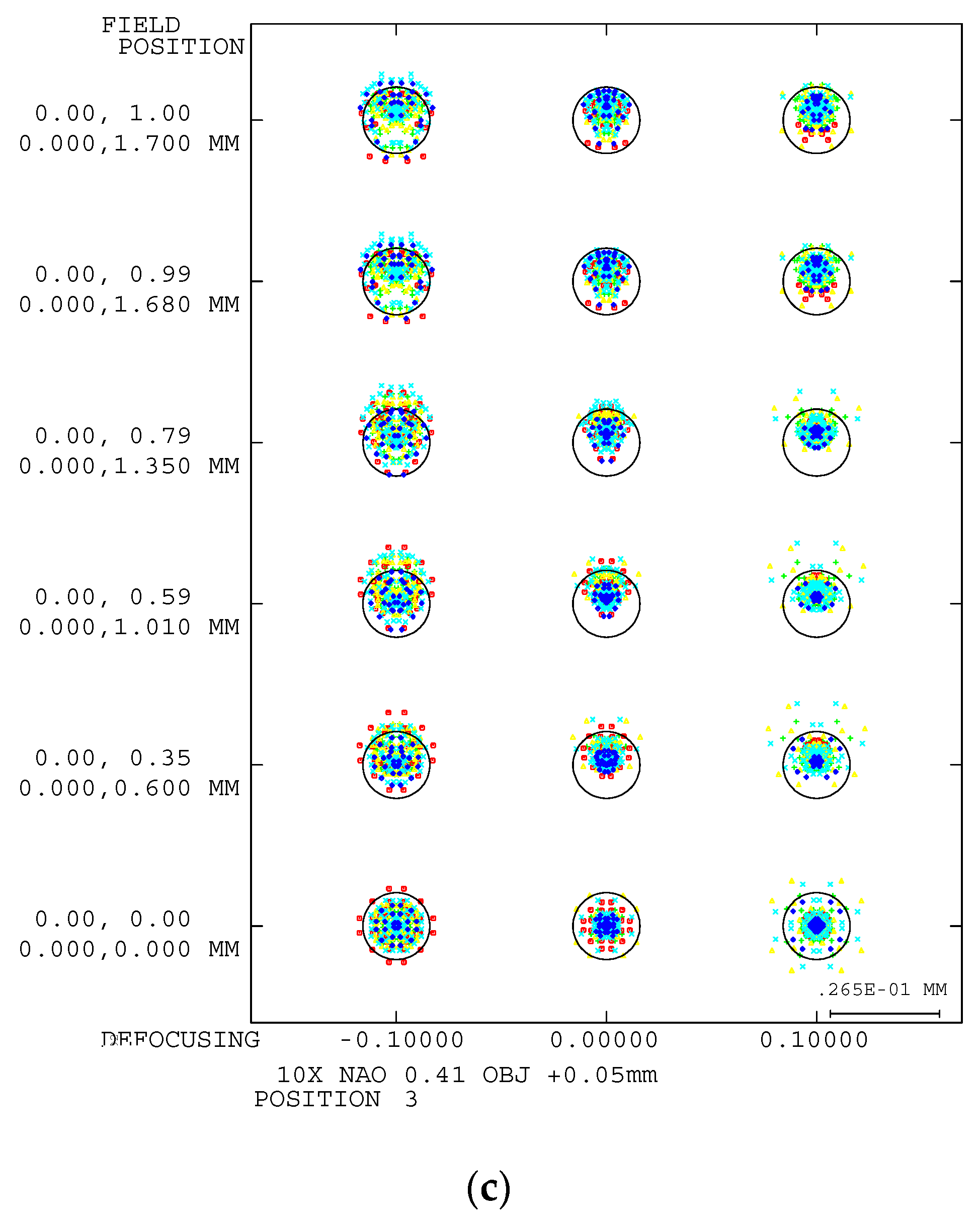
The sizes of the spots and airy disks were compared to evaluate the optical system resolution. The objective- and image-side NA of the optical system were 0.041 and 13.29 μm, respectively. Figure 8 shows the spot diagram of the 10× inspection optical system. A ray departing from one point on an object arrives at different locations in the image plane, depending on its pupil coordinates and wavelength. The spot diagram shows the degree to which each ray converges at a point in the image [52]. This indicates whether one point of an object can be seen as one point on the image plane; therefore, these data evaluate the resolution of the optical system [16]. In addition, the magnification of the optical system refers to the magnification at which the entire object is enlarged when it reaches the image plane. Figure 8a–c show spot diagrams based on the sample movement. In each spot diagram, the horizontal axis refers to the movement of the upper surface based on its position, whereas the vertical axis refers to the height of the object. An airy disk is a theoretically permissible circle of confusion that an image point can have [12]. When compared to the root mean square (RMS) of the distribution of the image points in the sports diagram, being close to the airy disk, which is the theoretical resolution limit, indicates that it has a high resolution [12]. In other words, a ray departing from one point on an object does not form an image at exactly one point on the image plane, depending on the pupil coordination and wavelength. The spot diagrams magnify these points to show the distribution of the rays. As listed in Table 1, the RMS represents the distribution when a ray departing from one point of an object reaches the image surface. The presented data refer to the spot RMS at the defocus 0.00 mm position without movement of the top surface of the spot diagram based on the sample movement, as shown in Figure 8a–c. The unit of the RMS is millimeters. The area marked with a black circle corresponds to the size of the airy disk; the diffraction-limited airy disk sets the standard for a high resolution [12]. As listed in Table 1, the largest RMS value is 7.67 μm and the size of the airy disk is 13.29 μm. The fact that the maximum spot size was smaller than that of the airy disk indicates that the light rays that started at one point converged at one point. In other words, it was observed that the designed 10× optical system had a high resolution.
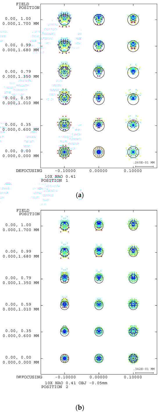
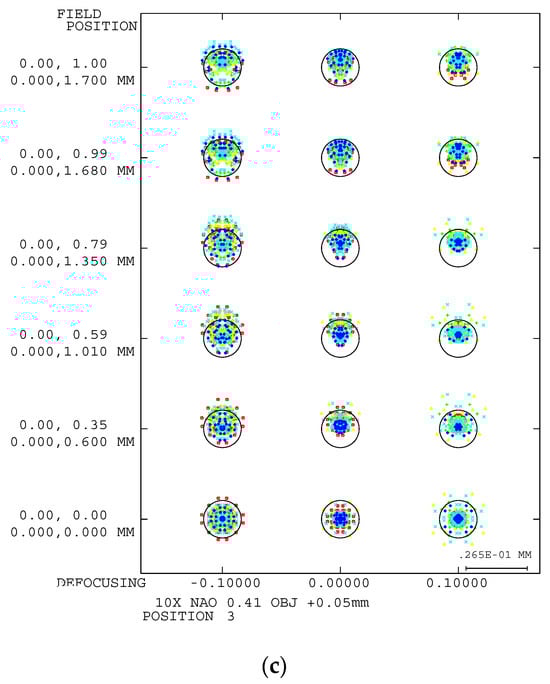
Figure 8.
Spot diagram of the 10× optical system when the sample moves (a) −0.36 mm from the reference point, (b) when the sample is located at the reference point, and (c) when the sample moves +0.36 mm.

Table 1.
Image RMS data of the 10× optical system.
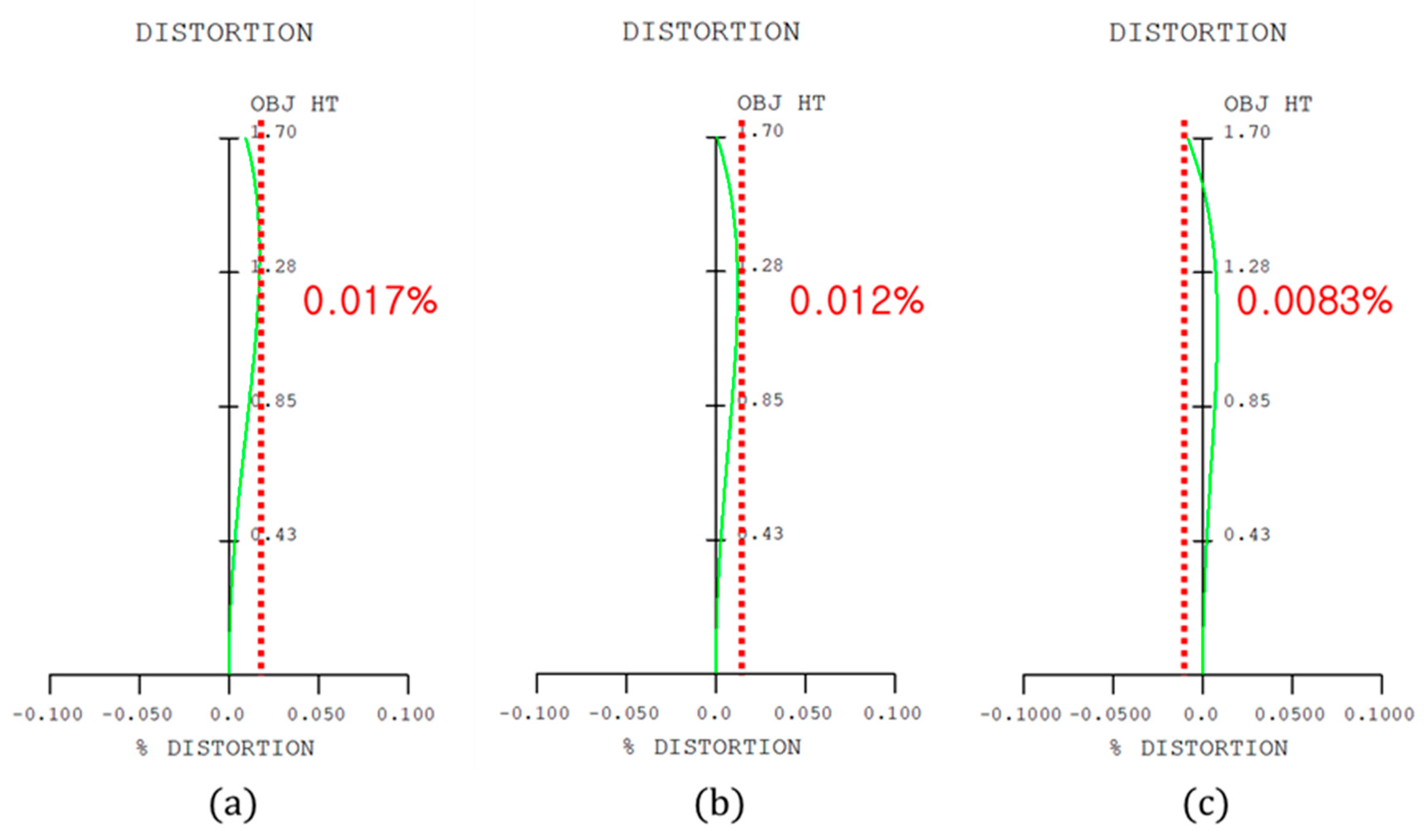
The optical inspection system was assumed free of distortion aberrations. Distortion refers to the difference between the height of the chief ray on the top plane and that of the chief ray considering aberrations in paraxial ray tracing [53]. The chief ray passes through the center of the aperture. Figure 9 shows the distortion aberration of the 10× optical system, which shows the distortion for object heights ranging from 0 to 1.7 mm. Figure 9a–c represent the distortion aberration diagram based on the sample movement. The X- and Y-axes represent the distortion aberration and sample height, respectively. We observe that the distortion aberration can be offset by combining the 30 mm focal length objective lens and the tube lens. Table 2 lists the actual data of the distortion aberration based on each sample height in position changes owing to sample movement, as shown in Figure 9a–c. As listed in Table 2, the largest RMS value is 9.73 μm. When the maximum spot size was compared to that of the airy disk, the maximum spot size was smaller. This implied that an image point could be viewed as a single point. In other words, we observed that the designed 5× optical system has a high resolution. As listed in Table 2, the maximum distortion aberration values (−0.017, 0.012, and 0.0083%) were close to zero.
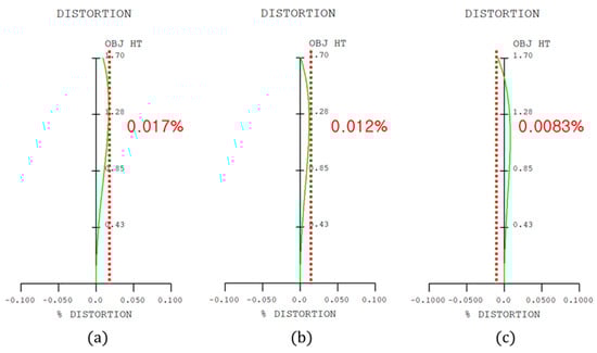
Figure 9.
Distortion aberration diagram of the 10× optical system when the sample moves (a) −0.36 mm from the reference point, (b) when the sample is located at the reference point, and (c) when the sample moves +0.36 mm.
Table 2.
Distortion aberration data of the 10× optical system.
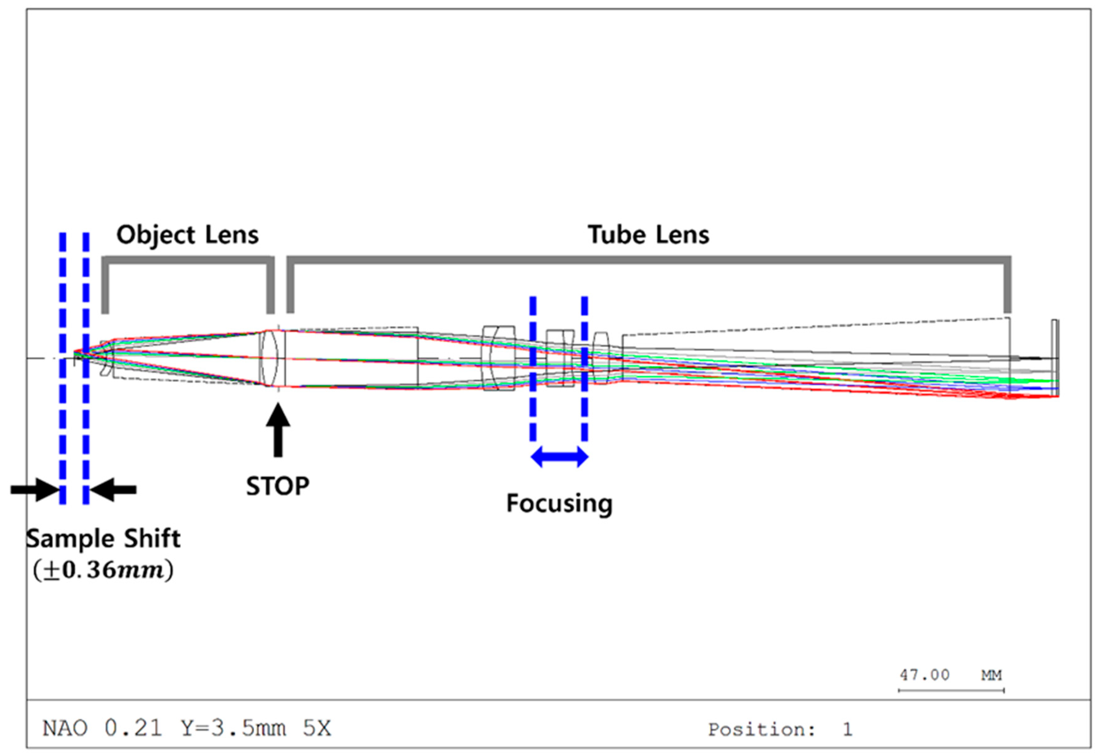
As the object moved by ±50 μm, the top surface moved. Using the internal focusing method, the movement of the lens group inside the optical system was calculated and applied to the image plane correction. Figure 10 shows the optical path diagram of the 5× optical system.
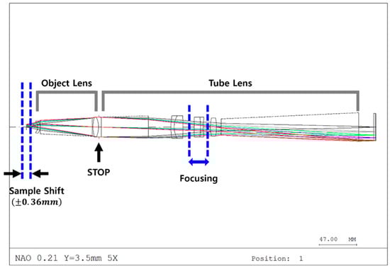
Figure 10.
Optical path diagram of the 5× optical system.
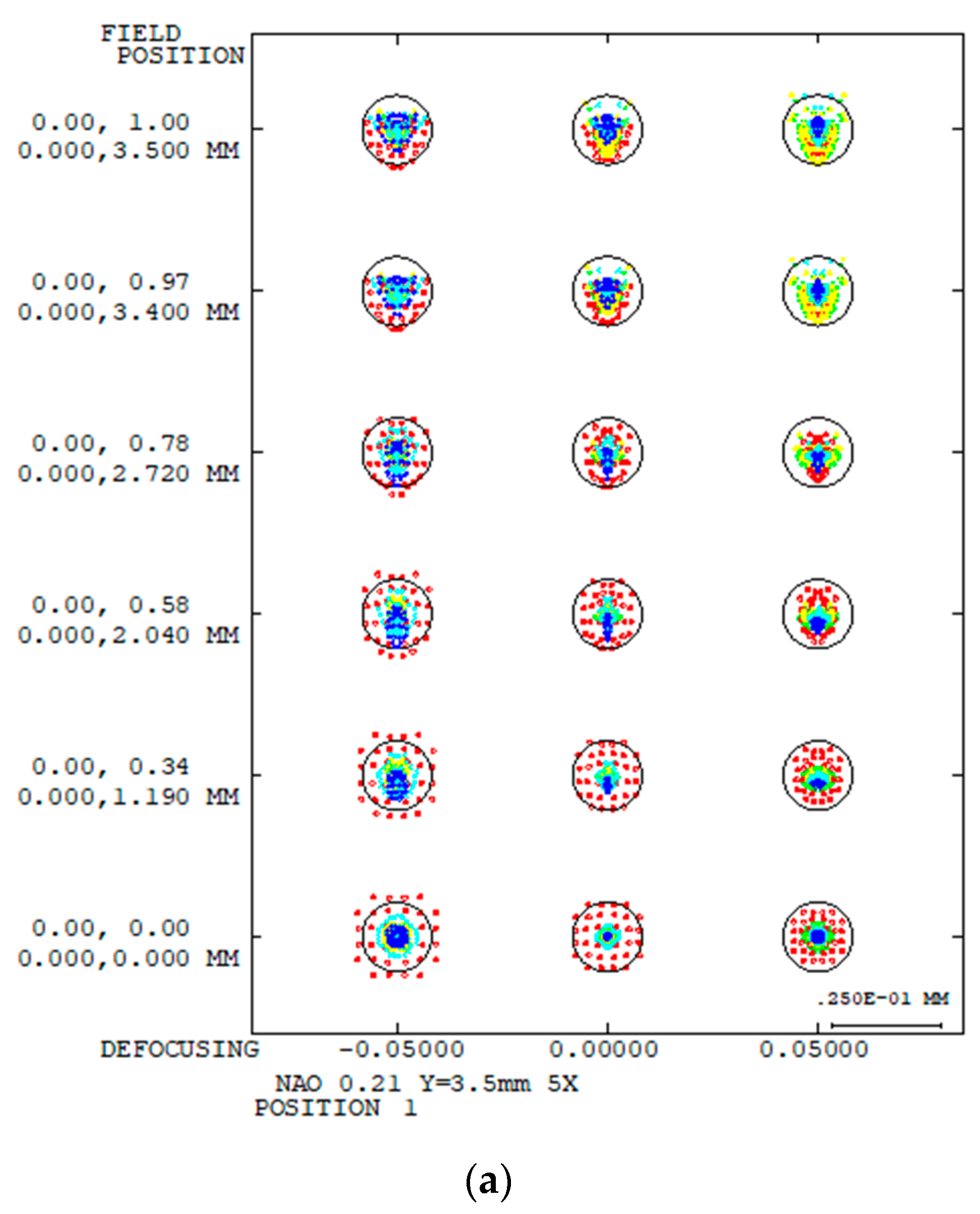
A spot diagram was created to analyze the resolution of the 5× inspection optical system. Figure 11 shows a spot diagram of the 5× optical system. Figure 11a–c show spot diagrams based on the sample movement. As in the 10× optical system, the airy disk of the 5× optical system is 13.29 μm and the black circles correspond to the size of the airy disk. In the spot diagram, the RMS of the image point size based on the sample size at a defocus of 0.00 mm without image point movement are listed in Table 3.
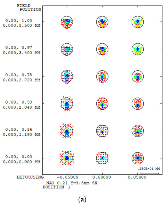
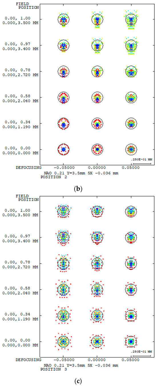
Figure 11.
Spot diagram of the 5× optical system when the sample moves (a) −0.36 mm from the reference point, (b) when the sample is located at the reference point, and (c) when the sample moves +0.36 mm.
Table 3.
Image RMS data of the 5× optical system.
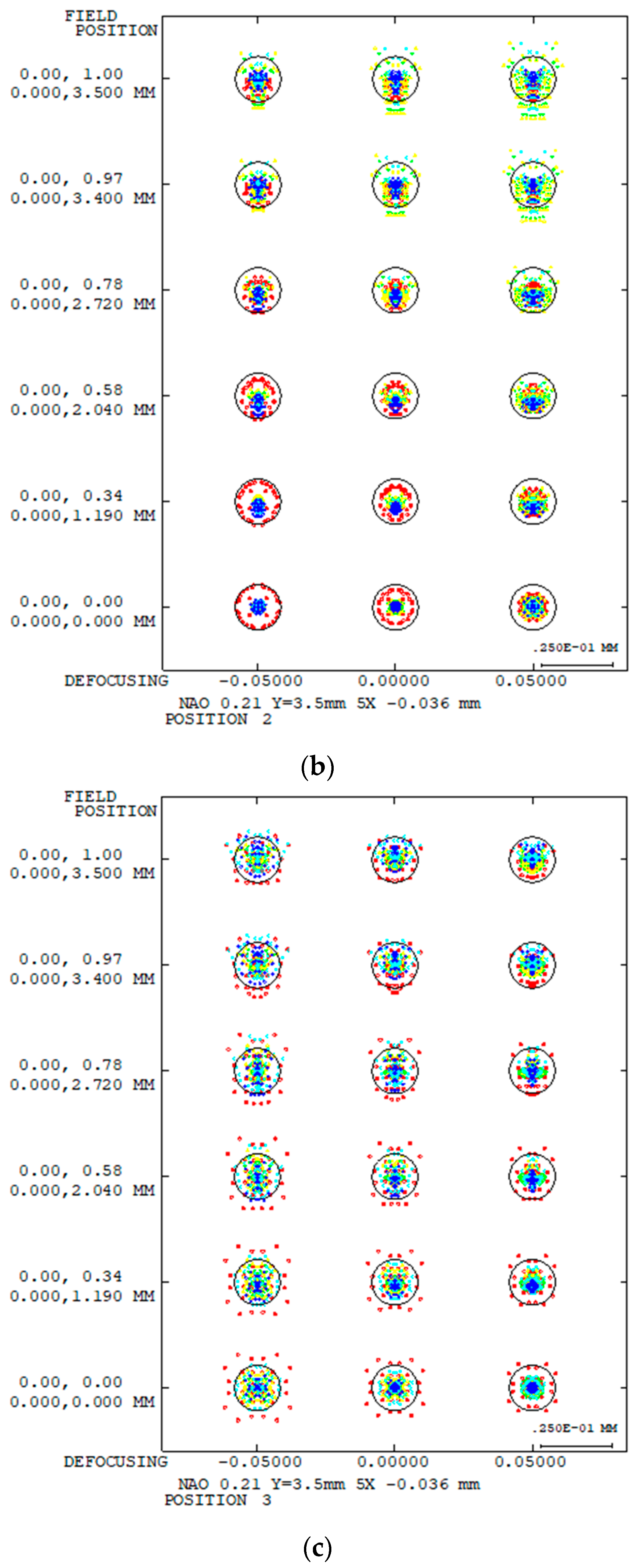
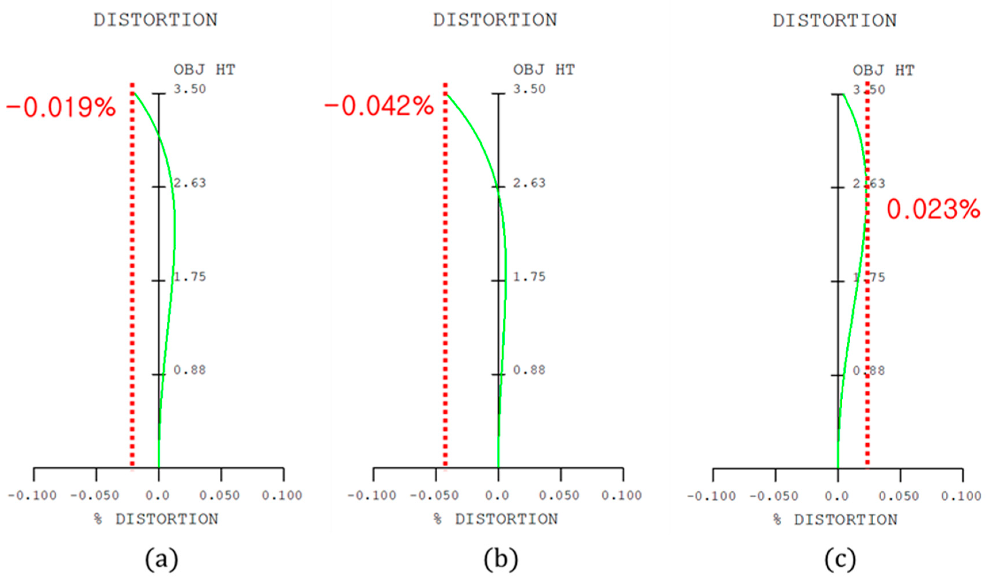
The distortion aberration was calculated to confirm that there was no distortion aberration in the 5× inspection optical system. The results confirm that most of the distortion aberration was canceled at –0.042. Figure 12 shows the distortion aberration diagram of the 5× inspection optical system, which indicates a distortion in the height of the object in the range of 0 to 3.5 mm. Figure 12a–c show the distortion aberration diagram based on the sample movement. The X- and Y-axes represent the distortion aberration and height of the sample, respectively. In addition, Table 4 lists the actual data on the distortion aberration based on each sample height in the position changes, as shown in Figure 12a–c. As listed in Table 4, the maximum distortion aberration values (−0.019, −0.042, and 0.023%) were close to zero.
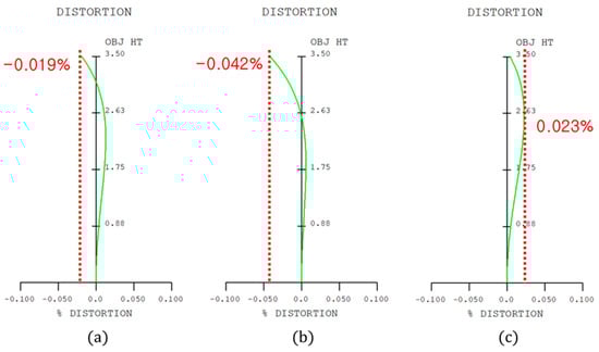
Figure 12.
Distortion aberration diagram of the 5× optical system when the sample moves (a) −0.36 mm from the reference point, (b) when the sample is located at the reference point, and (c) when the sample moves +0.36 mm.
Table 4.
Distortion of the 5× optical system.
4. Conclusions
In recent years, inspection optical systems have required an increasingly high resolution owing to the growth of the semiconductor market. To increase the resolution, a method of increasing the NA of the objective lens was considered. However, as the objective lens’s NA increases, the depth of focus decreases. To focus within the shortened depth of focus, the entire optical lens group has to be moved to maintain the resolution. As the size and weight of the lens-holding mechanism increase, so do the focusing time and the problems with inertial control and accuracy. However, to achieve a high resolution, the inspection optical system must be large and heavy, reducing the focusing speed and necessitating significant energy in the driving device to increase the speed.
To compensate for this, an internal focusing method was used rather than moving the entire optical system. A lens group for focusing was placed within the tube lens to widen its focus adjustment range. Thus, even when the sample’s position is changed, the internal focusing group moves to form an image on the image pickup device. However, when using this focusing method, the magnification may change depending on the object distance and optical system data change. Therefore, the optical system was designed as a telecentric collimator system in combination with objective and tube lenses. Using this setup, we confirmed that the magnification remained constant when the focus was adjusted based on sample movement.
In addition, a resolution analysis and performance evaluation were conducted using spot diagrams. As listed in Table 1 and Table 3, we confirmed that the spot size was similar to that of an airy disk. This design ensured that the distortion was offset when the objective and tube lenses were combined. This is because there should be no distortion aberration, owing to the characteristics of the optical inspection system. As listed in Table 2 and Table 4, the distortion aberration values were close to zero. The optical system’s resolution was set to be lower than that of the airy disk of 13.29 μm.
In the optical system, the weights of the objective lenses with focal lengths of 30 and 60 mm were calculated to be approximately 844 and 570 g, respectively, and the focusing group of the tube lens weighed approximately 22 g. These values confirm that the weight of the moving group can be significantly reduced, thereby reducing the inertial control by the weight of the focusing lens or the size of the actuator. The internal focus control method allows for faster and more accurate inspections than the current inspection optical system, which adjusts the entire optical lens group for focus. Therefore, we expect that the overall length of the optical system can be fixed, and the inspection device can be miniaturized. In addition, the inertia control by weight in the designed optical system is convenient.
Author Contributions
Conceptualization, D.J., J.P., J.R. and H.C.; methodology, D.J., J.P., J.R. and H.C.; writing—original draft preparation, D.J., J.P., J.R. and H.C. All authors have read and agreed to the published version of the manuscript.
Funding
This research was supported by Basic Science Research Program through the National Research Foundation of Korea (NRF) funded by the Ministry of Education (NRF-2020R1I1A3052712). This work was supported by the Gachon University research fund of 2023 (GCU-202304020001).
Institutional Review Board Statement
Not applicable for studies not involving humans or animals.
Informed Consent Statement
Not applicable for studies not involving humans.
Data Availability Statement
The data presented in this study are included in the article.
Conflicts of Interest
The authors declare no conflicts of interest. The funders had no role in the study’s design; collection, analyses, or interpretation of data; writing of the manuscript; or decision to publish the results.
References
- Fischer, R.; Tadic-Galeb, B.; Yoder, P. Optical System Design; McGraw-Hill Education: New York, NY, USA, 2008. [Google Scholar]
- Hecht, E.; Zajac, A. Optics; Addison Wesley: Boston, MA, USA, 1974; pp. 301–305. [Google Scholar]
- Walker, B.H. Optical Design for Visual Systems; SPIE Press: Bellingham, WA, USA, 2000. [Google Scholar]
- O’shea, D.C.; C’Shea, D.C. Elements of Modern Optical Design; Wiley Publishing: Hoboken, NJ, USA, 1985. [Google Scholar]
- Bass, M.; Van Stryland, E.W.; Williams, D.R.; Wolfe, W.L. Handbook of Optics; McGraw-Hill Education: New York, NY, USA, 2001. [Google Scholar]
- Gross, H.; Blechinger, F.; Achtner, B. Handbook of Optical Systems; Wily-VCH Verlag GmbH & Co.: Hoboken, NJ, USA, 2005. [Google Scholar]
- Welford, W.T. Aberrations of Optical Systems; CRC Press: Boca Ration, FL, USA, 1986. [Google Scholar]
- Ray, S. Applied Photographic Optics; Routledge: Oxfordshire, UK, 2002. [Google Scholar]
- Smith, W.J. Modern Optical Engineering; McGraw-Hill Education: New York, NY, USA, 2007. [Google Scholar]
- Zappe, H. Fundamentals of Micro-Optics; Cambridge University Press: Cambridge, UK, 2010. [Google Scholar]
- Twyman, F. Prism and Lens Making: A Textbook for Optical Glassworkers; Routledge: Abingdon-on-Thames, UK, 2017. [Google Scholar]
- Airy, G.B. On the diffraction of an object-glass with circular aperture. Trans. Camb. Philos. Soc. 1835, 5, 283. [Google Scholar]
- Ippolito, S.; Goldberg, B.; Ünlü, M. Theoretical analysis of numerical aperture increasing lens microscopy. J. Appl. Phys. 2005, 97, 053105. [Google Scholar] [CrossRef]
- Iga, K.; Kokubun, Y. Encyclopedic Handbook of Integrated Optics; CRC Press: Boca Raton, FL, USA, 2005. [Google Scholar]
- Kidger, M.J. Intermediate Optical Design; SPIE Publications: Bellingham, WA, USA, 2004. [Google Scholar]
- Klingshirn, C.F. Semiconductor Optics; Springer Science & Business Media: Berlin, Germany, 2012. [Google Scholar]
- Schäfer, W.; Wegener, M. Semiconductor Optics and Transport Phenomena; Springer Science & Business Media: Berlin, Germany, 2013. [Google Scholar]
- Kim, B.-T.; Hyun, D.-H.; Yoo, K.-S. Ultra-precision High Numerical Aperture Plastic Objective Lens for Blu-ray Disc Pick-up. J. Korean Soc. Manuf. Technol. Eng. 2011, 20, 811–816. [Google Scholar]
- Chee, S.; Ryu, J.; Choi, H. New Optical Design Method of Floating Type Collimator for Microscopic Camera Inspection. Appl. Sci. 2021, 11, 6203. [Google Scholar] [CrossRef]
- Herzberger, M. Gaussian optics and Gaussian brackets. J. Opt. Soc. Am. 1943, 33, 651–655. [Google Scholar] [CrossRef]
- Mikš, A.; Novák, J.; Novák, P. Method of zoom lens design. Appl. Opt. 2008, 47, 6088–6098. [Google Scholar] [CrossRef]
- Kim, K.M.; Choe, S.-H.; Ryu, J.-M.; Choi, H. Computation of Analytical Zoom Locus Using Padé Approximation. Mathematics 2020, 8, 581. [Google Scholar] [CrossRef]
- Jung, U.; Choi, J.H.; Choo, H.T.; Kim, G.U.; Ryu, J.; Choi, H. Fully Customized Photoacoustic System Using Doubly Q-Switched Nd: YAG Laser and Multiple Axes Stages for Laboratory Applications. Sensors 2022, 22, 2621. [Google Scholar] [CrossRef] [PubMed]
- Fischer, R.E. Fundamentals of HMD Optics; McGraw-Hill: New York, NY, USA, 1997. [Google Scholar]
- Clark, A.D.; Wright, W. Zoom Lenses; Adam Hilger Ltd.: London, UK, 1973. [Google Scholar]
- Smith, G.H. Practical Computer-Aided Lens Design; Willmann-Bell, Incorporated: Richmond, VA, USA, 1998. [Google Scholar]
- Choi, H.; Cho, S.; Ryu, J. Novel Telecentric Collimator Design for Mobile Optical Inspection Instruments. Curr. Opt. Photonics 2023, 7, 263–272. [Google Scholar]
- Figl, M.; Ede, C.; Hummel, J.; Wanschitz, F.; Ewers, R.; Bergmann, H.; Birkfellner, W. A fully automated calibration method for an optical see-through head-mounted operating microscope with variable zoom and focus. IEEE Trans. Med. Imaging 2005, 24, 1492–1499. [Google Scholar] [CrossRef] [PubMed]
- Park, S.C.; Shannon, R.R. Zoom lens design using lens modules. Opt. Eng. 1996, 35, 1668–1676. [Google Scholar] [CrossRef]
- Pedrotti, F.L.; Pedrotti, L.S. Introduction to Optics; Prentice-Hall: Englewood Cliffs, NJ, USA, 1993; Volume 2. [Google Scholar]
- Osten, W. Optical inspection of Microsystems; CRC Press: Boca Raton, FL, USA, 2019. [Google Scholar]
- Choi, Y.-C.; Rim, C.-S. Design of a telecentric lens with a smartphone camera to utilize machine vision. Korean J. Opt. Photonics 2018, 29, 149–158. [Google Scholar]
- Mikš, A.; Novák, J. Method of initial design of a two-element double-sided telecentric optical system. Opt. Express 2023, 31, 1604–1614. [Google Scholar] [CrossRef] [PubMed]
- Li, J.; Zhang, K.; Du, J.; Li, F.; Yang, F.; Yan, W. Design and theoretical analysis of the image-side telecentric zoom system using focus tunable lenses based on Gaussian brackets and lens modules. Opt. Lasers Eng. 2023, 164, 107494. [Google Scholar] [CrossRef]
- Li, J.; Zhang, K.; Du, J.; Li, F.; Yang, F.; Yan, W. Double-sided telecentric zoom optical system using adaptive liquid lenses. Opt. Express 2023, 31, 2508–2522. [Google Scholar] [CrossRef]
- Chang, C.-L.; Huang, K.-C.; Wu, W.-H.; Lin, Y.-H. The design and fabrication of telecentric lens with large field of view. In Proceedings of the Current Developments in Lens Design and Optical Engineering XI; and Advances in Thin Film Coatings VI, San Diego, CA, USA, 1–3 August 2010; SPIE: San Diego, CA, USA, 2010; pp. 241–247. [Google Scholar]
- Zhimuleva, E.; Zavyalov, P.; Kravchenko, M. Development of telecentric objectives for dimensional inspection systems. Optoelectron. Instrum. Data Process. 2018, 54, 52–60. [Google Scholar] [CrossRef]
- Zhong, Y.; Tang, Z.; Gross, H. Correction of 2D-telecentric scan systems with freeform surfaces. Opt. Express 2020, 28, 3041–3056. [Google Scholar] [CrossRef]
- Li, X.; Zou, C.; Yang, J. Design of image-side telecentric off-axis three-mirror anastigmatic systems based on the coaxial parent mirrors. Optik 2021, 241, 166855. [Google Scholar] [CrossRef]
- Liu, X.; Liu, H. Research on design method of spaceborne imaging spectrometer system based on telecentric optical system. In Proceedings of the 2015 International Conference on Optical Instruments and Technology: Optical Systems and Modern Optoelectronic Instruments, Beijing, China, 17–19 May 2015; SPIE: Beijing, China, 2015; pp. 341–346. [Google Scholar]
- Liu, S.; Sun, G.; Zhang, G.; Chen, S.; Chen, J.; Zhang, J. Optical Design of a Solar Simulator With Large Irradiation Surface and High Irradiation Uniformity. IEEE Photonics J. 2022, 14, 1–9. [Google Scholar]
- Xu, D.; Chaudhuri, R.; Rolland, J.P. Telecentric broadband objective lenses for optical coherence tomography (OCT) in the context of low uncertainty metrology of freeform optical components: From design to testing for wavefront and telecentricity. Opt. Express 2019, 27, 6184–6200. [Google Scholar] [CrossRef]
- Choi, H.; Ryu, J.-M.; Choe, S.-W. A novel therapeutic instrument using an ultrasound-light-emitting diode with an adjustable telephoto lens for suppression of tumor cell proliferation. Measurement 2019, 147, 106865. [Google Scholar] [CrossRef]
- Choi, H.; Jo, J.; Ryu, J.-M.; Yeom, J.-Y. Ultrawide-angle optical system design for light-emitting-diode-based ophthalmology and dermatology applications. Technol. Health Care 2019, 27 (Suppl. S1), 133–142. [Google Scholar] [CrossRef] [PubMed]
- Thibault, S.; Gauvin, J.; Doucet, M.; Wang, M. Enhanced optical design by distortion control. In Proceedings of the Optical Design and Engineering II, Jena, Germany, 13–16 September 2005; SPIE: Jena, Germany, 2005; pp. 307–314. [Google Scholar]
- Mahajan, V.N. Optical Imaging and Aberrations: Part I: Ray Geometrical Optics; SPIE Press: Bellingham, WA, USA, 1998. [Google Scholar]
- Smith, W.J. Modern Lens Design; McGraw-Hill New York: New York, NY, USA, 2005. [Google Scholar]
- Laikin, M. Lens Design; CRC Press: Boca Raton, FL, USA, 2006. [Google Scholar]
- Choi, H.; Ryu, J.M.; Kim, J.H. Tolerance Analysis of Focus-adjustable Head-mounted Displays. Curr. Opt. Photonics 2017, 1, 474–490. [Google Scholar]
- Choi, H.; Ryu, J.-M.; Yeom, J.-Y. Development of a Double-Gauss Lens Based Setup for Optoacoustic Applications. Sensors 2017, 17, 496. [Google Scholar] [CrossRef]
- Mouroulis, P.; Macdonald, J. Geometrical Optics and Optical Design; Oxford University Press: New York, NY, USA, 1997. [Google Scholar]
- Yamaji, K. Progress in Optics; Elsevier: Amsterdam, The Netherlands, 1967. [Google Scholar]
- Prescott, B.; McLean, G. Line-based correction of radial lens distortion. Graph. Models Image Process. 1997, 59, 39–47. [Google Scholar] [CrossRef]


Disclaimer/Publisher’s Note: The statements, opinions and data contained in all publications are solely those of the individual author(s) and contributor(s) and not of MDPI and/or the editor(s). MDPI and/or the editor(s) disclaim responsibility for any injury to people or property resulting from any ideas, methods, instructions or products referred to in the content. |
© 2024 by the authors. Licensee MDPI, Basel, Switzerland. This article is an open access article distributed under the terms and conditions of the Creative Commons Attribution (CC BY) license (https://creativecommons.org/licenses/by/4.0/).