Article

Real-Time Adjustment Method for Metro Systems with Train Delays Based on Improved Q-Learning

1
College of Applied Technology, Shenzhen University, Shenzhen 518060, China
2
College of Urban Transportation and Logistics, Shenzhen Technology University, Shenzhen 518063, China
*
Author to whom correspondence should be addressed.
Appl. Sci. 2024, 14(4), 1552; https://doi.org/10.3390/app14041552
Submission received: 28 December 2023 / Revised: 7 February 2024 / Accepted: 12 February 2024 / Published: 15 February 2024

Abstract

:
This paper presents a solution to address the challenges of unexpected events in the operation of metro trains, which can lead to increased delays and safety risks. An improved Q-learning algorithm is proposed to reschedule train timetables via incorporating train detention and different section running times as actions. To enhance computational efficiency and convergence rate, a simulated annealing dynamic factor is introduced to improve action selection strategies. Additionally, importance sampling is employed to evaluate different policies effectively. A case study of Shenzhen Metro is conducted to demonstrate the effectiveness of the proposed method. The results show that the method achieves convergence, fast computation speed, and real-time adjustment capabilities. Compared to traditional methods such as no adjustment, manual adjustment, and FIFO (First-In-First-Out), the proposed method significantly reduces the average total train delay by 54% and leads to more uniform train headways. The proposed method utilizes a limited number of variables for practical state descriptions, making it well suited for real-world applications. It also exhibits good scalability and transferability to other metro systems.

1. Introduction

In today’s urbanization process, tunnels have become an essential component of urban infrastructure due to the increasingly constrained urban space. Tunnels play a critical role in various domains, including transportation, water supply, and energy transmission, significantly improving the efficiency of urban operations [1]. Specifically, in the transportation field, the rapid development of metro systems, which are built upon tunnel engineering, has effectively mitigated the mounting traffic congestion in densely populated areas. Moreover, metro systems effectively meet the growing transportation needs of densely populated areas.
However, along with this development comes a set of challenges, with train delays being particularly prominent. As metro lines and infrastructure age, the occurrence of train delays tends to increase, especially during peak hours. These delays have far-reaching consequences, impacting the functioning of the city and the daily routines of its residents. Train delays are not merely operational issues, they have a significant impact on passenger services and the overall efficiency of the metro system. Delays disrupt passenger travel plans, cause frustration, and reduce the overall capacity of the trains, leading to dissatisfaction and complaints from passengers. Moreover, delays pose a safety risk, especially during crowded peak hours, as sudden incidents can result in stampedes or other accidents.
Train delays are a frequent and significant problem in metro operations, occurring when trains deviate from their scheduled arrival or departure times. Various factors contribute to these delays, including equipment malfunctions (such as issues with the catenary, signal system failures, or vehicle breakdowns), human factors (such as passenger misconduct or obstructions), adverse weather conditions (such as heavy rain, snowstorms, or thunderstorms), and planned maintenance activities [2]. To effectively manage train delays, they are often categorized based on their duration. Minor delays are typically brief, lasting only a few minutes, and are often caused by minor issues like temporary signal failures or slow passenger boarding and alighting. Moderate delays encompass a range of several minutes to half an hour and involve more complex challenges such as equipment malfunctions, adverse weather conditions, or traffic accidents. Severe delays are the most significant, lasting for more than half an hour and potentially extending to several hours. They are often the result of major equipment failures, severe weather events, or significant traffic accidents, requiring an extended period to restore normal operations. In cases where a train experiences prolonged delays due to external disruptions, train dispatchers can address the recovery process by selectively canceling certain trains and modifying train routes [3].
Currently, the handling of metro train delays heavily relies on the experience of dispatchers and manual interventions [4]. However, as metro systems continue to expand, the effectiveness and accuracy of manual delay management face challenges. Therefore, there is an urgent need to explore intelligent and efficient methods to respond to delays. Technological support is crucial in addressing metro train delay issues, as it can enhance the operational stability of metro systems and ensure passenger safety and satisfaction. Through employing advanced technologies and intelligent systems, metro operators can better manage and respond to train delays, leading to an improved operational efficiency, enhanced safety measures, and a better overall travel experience for passengers. This paper proposes a new method using an improved Q-learning algorithm to assist metro staff to deal with train delays.

1.1. Literature Review

For train timetable adjustments in delay scenarios, scholars such as Cacchiani have summarized it as the train timetable rescheduling (TTR) problem [5]. TTR involves modifying train operations by altering the sequence of trains, departure/arrival times, tracks/stations, etc., with the objective of reducing train delays. This adjustment is crucial for enhancing the quality of train services and improving passenger experiences. However, the TTR problem falls under the category of NP-Hard, indicating that it is a highly challenging problem that cannot be easily solved within affordable time in computational theory. As the problem’s scale increases, the number of variables and constraints in TTR grows exponentially, making it exceedingly difficult to find rapid solutions for the model [5,6,7]. It is worth noting that compared to other scheduling problems like job shop scheduling, the TTR problem requires higher decision-making efficiency to ensure the safety and operational efficiency of trains [8]. Moreover, train operation adjustments have stringent real-time requirements, implying accurate modifications to be made within a short timeframe. The inherent conflict between these two aspects has made finding rapid solutions to the train timetable adjustment problem a long-standing focus and a significant challenge in research.
Currently, researchers have put forward multiple solutions to address the TTR problem. Fang et al. conducted a comprehensive review on this matter and suggested a hybrid approach as a future development direction. They also expressed the need for new methods in future research [9]. In line with this, the present article incorporates novel machine learning techniques and broadly categorizes the existing research methods into the following five categories: manual adjustment methods, optimization model methods, simulation methods, optimization methods based on heuristic algorithms, and AI methods.
Manual adjustment methods are currently more commonly used in practice. Existing manual rule-based methods include First-Come-First-Serve (FCFS) [10], First-Schedule-First-Serve (FSFS) [11], and First-In-First-Out (FIFO) [12]. However, designing efficient scheduling remains a challenging task. Dispatchers face the crucial question of how to devise a high-performance and cost-effective method.
Optimization model methods generally employ different planning models to describe the TTR problem, including integer programming [13], mixed-integer linear programming [14], constraint programming [15], and quadratic programming methods [16]. Scholars have applied specialized algorithms, such as branch and bound (B and B) [17] and branch and price [18], to tackle these planning models, decomposing the complex problem into simpler ones. Although this approach can provide precise solutions, the response time tends to be relatively long. To address this issue, researchers have proposed novel targeted algorithms, including parallel algorithms [7], decomposition methods [19,20], rolling time domain algorithms [21], traffic direction multiplier methods [19,22], and heuristic-assisted methods [23,24], aiming to reduce computational costs.
Simulation methods, such as train movement models based on the following theory, are used to test control algorithms and design solutions for train operations. For instance, Li designed a train movement model under a fixed block signaling system [25]. Xun et al. further developed a railway traffic cellular automaton model under a moving block signaling system [26]. Corman et al. extended traffic flow models to railways using a stochastic process model [27]. Ketphat et al. introduced a train operation model under a virtual coupling system [28]. Saeid et al. presented a mesoscopic train-following model that accurately captures train interactions and predicts delays based on train spacing [29]. These simulation methods are known for their realism and accuracy, but face challenges related to complex modeling and computational requirements.
Heuristic algorithms are also employed to provide optimization solutions in TTR. Various metaheuristic approaches have been extensively studied, including taboo search [30], genetic algorithms [31], particle swarm algorithms [32], and ant colony algorithms [33]. Within this field, many scholars have designed specific operators to handle problem constraints. Compared to optimization model methods and simulation methods, heuristic algorithms offer greater flexibility, faster computation, and the ability to handle complex problems.
AI methods have gained popularity in addressing the TTR problems. Recognizing the limitations of heuristic algorithms, such as their susceptibility to local optima and poor adaptability, researchers are now exploring machine-learning-based methods. Machine-learning-based methods can be further divided into three main types:
(1)
The first type involves understanding the search process of existing search algorithms. For example, Qu et al. employed reinforcement learning to solve the process of mixed-integer linear programming, designing a reinforcement-learning-based branching strategy [34]. Tang et al. used reinforcement learning to select appropriate cutting planes for the branch-and-cut process [35].
(2)
The second type is based on data-driven approaches. For instance, Dündar et al. combined genetic algorithms with artificial neural networks to simulate train dispatchers in conflict resolution [36]. However, these methods may not be suitable for solving the TTR problem efficiently due to their extended response times.
(3)
The third type involves using reinforcement learning to directly construct solution strategies, which is more suitable for the TTR problem. In the field of railway operations, D. Šemrov was among the early adopters of the Q-learning algorithm to tackle the single-track train rescheduling problem. However, challenges arose due to the large state vector and scalability issues to other scenarios [37]. Harshad Khadilkar extended the Q-learning algorithm to real-world instances of single-track and multi-track dispatch, reducing the state vector representation and enhancing scalability. Real-time computation remained a challenge [38]. Zhu et al. employed Q-learning to solve the railway timetable rescheduling problem and demonstrated its effectiveness in finding high-quality solutions within a limited training set [39]. Li et al. utilized a multi-agent deep reinforcement learning approach for the TTR problem. However, their method lacked delay information, had limited state generality, and exhibited insufficient scalability [40]. Ning expanded the state representation to include the actual arrival and departure times of trains, providing more information about delays [41]. Some scholars found that learning strategies could only be trained for individual problem instances. For example, Ghasempour et al. trained learning strategies from multiple instances to address delay scenarios at railway intersections [42]. Wang et al. used a policy-based reinforcement learning approach, but their problem only allowed for the delay of one train, which does not capture the simultaneous delays of multiple trains that often occur in reality [43]. In the field of metro systems, Su et al. used Q-learning to simulate metro train operations and adjust schedules. However, their state definition made it challenging to solve large-scale scenarios, leading to the risk of local optima or difficulties in problem-solving [44]. Liao et al. proposed using deep reinforcement learning (DRLA) to minimize energy consumption in metro train timetable rescheduling [45].
In summary, each method has its strengths and limitations. A comparison between these methods and the proposed approach in this paper is provided in Table 1.
Upon analyzing the literature, it becomes apparent that previous studies on the TTR problem have certain limitations. When applying certain algorithms to tackle this problem, there are issues related to incomplete model construction. Some specific problems include:
(1)
Manual adjustment methods rely on the experience and manual intervention of dispatchers when dealing with train delays. However, these methods are constrained by the formulation and adaptability of manual rules, which makes it difficult to cope with the complexity and variability of actual operational scenarios. Optimization model methods can simulate train operations through complex algorithms, but they often struggle to accurately capture various complex factors in real-world scenarios. Simulation methods attempt to predict via simulating the interactions between trains, but they face computational complexity challenges when dealing with large-scale networked operations, making it difficult to rapidly solve problems with high real-time requirements. Heuristic algorithms are prone to getting stuck in local optima and often require significant computation time.
(2)
Reinforcement learning has gained considerable attention. Through interactive learning between intelligent agents and the environment, reinforcement learning gradually optimizes decision-making strategies, exhibiting adaptability and intelligence. In the field of metro systems, utilizing reinforcement learning to directly construct solution strategies can better adapt to the complexity and variability of actual operational scenarios.
(3)
Currently, most reinforcement learning methods focus on cases where only a single train is delayed, neglecting scenarios where multiple trains experience simultaneous delays, failing to consider the interactions between trains. Furthermore, existing methods often involve complex state representations, which can lead to inefficient problem-solving processes and challenges in ensuring real-time accuracy and prediction.

1.2. Contribution of This Paper

Based on the analysis provided, this paper proposes an improved Q-learning algorithm that specifically addresses scenarios where multiple trains experience delays simultaneously. The algorithm focuses on several key aspects to enhance its practical applicability in metro train delay issues. The contributions of this paper are outlined as follows:
(1)
The proposed algorithm narrows down the scope of state variables, providing a clear and concise description of delay situations, which facilitates efficient real-time processing to improve its effectiveness in practical applications.
(2)
A simulated annealing dynamic factor is introduced to improve convergence stability and computation speed.
(3)
This algorithm is trained on scenarios involving delayed interaction between multiple trains, improving its universality and portability.
The structure of this paper is as follows: Section 2 explores the delay process of trains and the measures taken during train delays. Section 3 models the problem of train delays, constructs the objective function, and defines the corresponding constraints. Section 4 proposes the use of the improved Q-learning algorithm to address the TTR problem. Section 5 evaluates the algorithm’s effectiveness through case studies. The final section summarizes the advantages and significance of this paper.

2. Problem Description

2.1. Train Operation and Train Delay

Metro train operations involve the movement of trains between stations along railway tracks, which consist of multiple blocks. Here, a metro station refers to a physical station where passengers board and alight from trains, while virtual stations are defined as the boundary points between two adjacent blocks along the railway tracks. To ensure safe and efficient operations, specific running times are calculated for different blocks of a metro line, taking into account factors such as curves, slopes, switches, and distances between stations. These running times are categorized into different block running time levels, each associated with a recommended speed curve [46]. This comprehensive management and scheduling approach ensures the smooth operation of the metro transit system, ultimately providing passengers with an enhanced travel experience. The relationship between block running time levels and the corresponding recommended speed curve is depicted in Figure 1.
Train delays are the phenomenon whereby trains deviate from their scheduled arrival or departure times, caused by some unexpected events. When addressing train delay issues, it is crucial to understand how delays propagate throughout the system [47]. The impact of delay events can be categorized into three stages: initial delay, secondary delay, and delay propagation, as illustrated in Figure 2. In the figure, the horizontal axis represents time, while the vertical axis represents the physical stations and the virtual stations. Physical stations are represented by a solid green line, while virtual stations are denoted by dashed lines. The black line represents the initial train schedule, while the red dashed line illustrates the adjusted actual train schedule, reflecting deviations resulting from delays. Furthermore, the blue dashed line represents a modified train schedule with different block running time levels, indicating potential adjustments aimed at mitigating delays.
In Figure 2, the initial delay occurs when the first train fails to depart according to its original timetable at the fourth physical station. It signifies the first occurrence of a train deviating from its scheduled departure time. The secondary delay manifests as a consequence of the initial delay. It may lead to a reduction in the train headway or necessitate the waiting of other trains for the delayed train, thus affecting their planned operations. This propagation of delays refers to the gradual expansion of the initial delay. When a train experiences significant delays, it can trigger a chain reaction, subsequently causing delays in subsequent trains and affecting an increasing number of trains over time. This propagation phenomenon spreads throughout the transportation network, disrupting the normal operation of the system.

2.2. Measures for Train Delays

When dealing with train delays, the requirement of real-time becomes crucial. In situations with longer delays, flexible measures like train service cancellations or route adjustments can be implemented to mitigate the overall impact of delays on the system. However, in situations with short-term delays, the timely rescheduling of the train timetable becomes essential as it directly affects the operational efficiency and safety of the metro system.
Without staff adjustments, the metro system would continue operating based on the original plan, resulting in subsequent trains experiencing the same delay as the first train. This cumulative effect would lead to significantly longer overall delay times. To prevent this accumulation, staff members, following the metro’s emergency plan, assess the delay situation of the first train and progressively detain subsequent trains to ensure safe operation and to address timetable adjustment issues. However, manual adjustment often requires a long dwelling time and may lead to uneven adjustments across multiple trains and physical stations. In addition, the First-In-First-Out (FIFO) algorithm is commonly used for rescheduling. This algorithm arranges departures based on the order in which trains enter the physical station, maintaining the original entry order. However, the FIFO algorithm does not consider factors such as train priority or the degree of delay, which might result in suboptimal rescheduling plans.
To address train delays, this paper proposes a new method that comprehensively considers multiple factors, including train priority and delay conditions. The decision variables are the physical station dwelling times of subsequent trains, and the section running times with different block running time levels. When delays occur, strategies such as increasing the dwelling time of subsequent trains at physical stations or modifying trains’ block running time level can be adopted. The goal is to provide a more practical solution for real-time train adjustments.

3. Model Construction

3.1. Model Notations and Assumptions

In this section, we will provide the mathematical description of the TTR problem. Table 2 presents the list of symbols to be used.
The metro line studied in this paper involves regular bi-directional operations, including both upstream and downstream directions with turnaround stations, as shown in Figure 3. In the figure, the set of stations is represented by I , while the set of physical stations is denoted by I . Solid circles represent physical stations, while hollow circles represent virtual stations. The stations between station I and I + 1 , as well as between station 2 I and 1 , serve as turnaround stations.
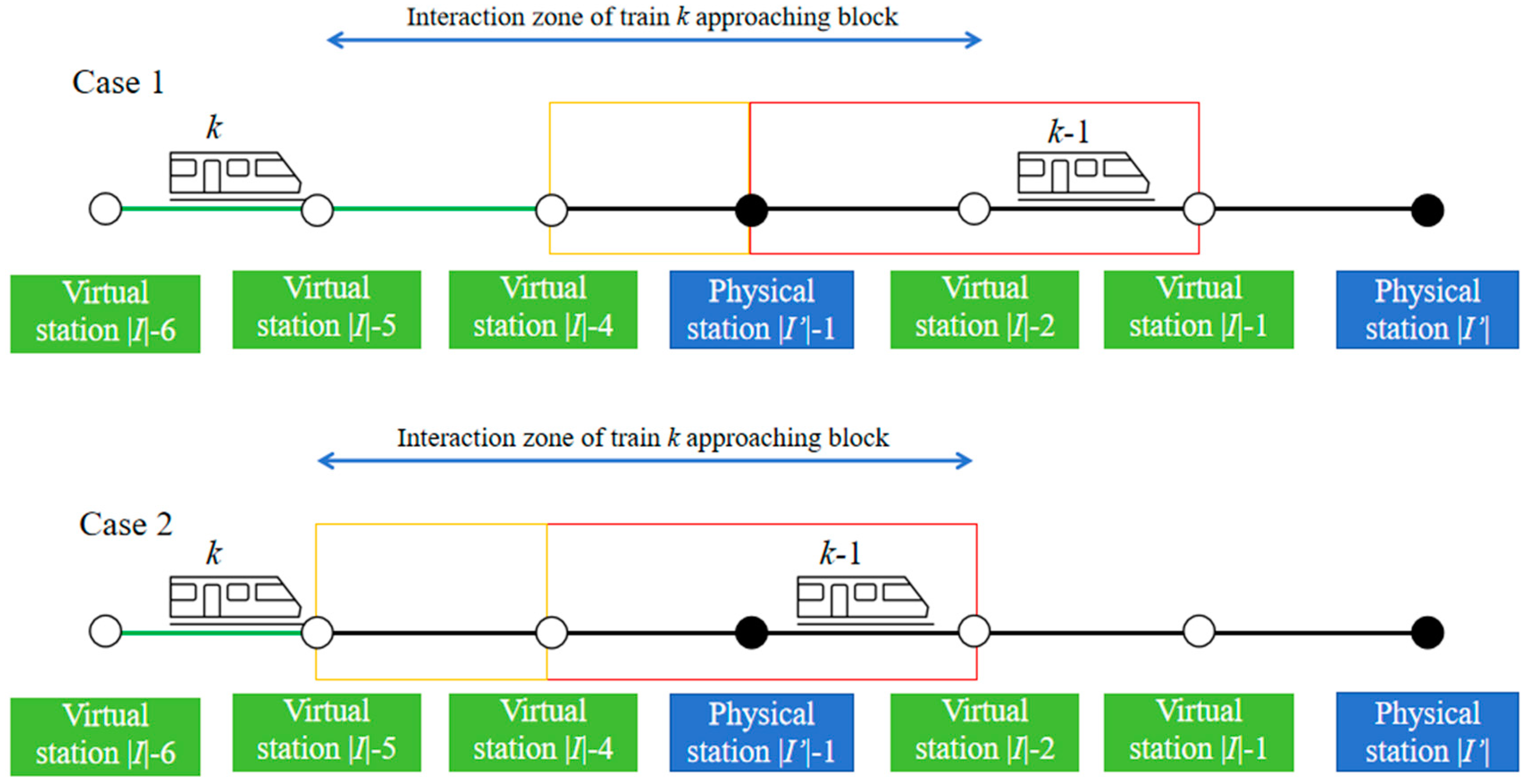
Under normal circumstances, metro trains operate in CBTC (communication-based train control) mode. However, the metro signal system utilizes a fixed-block system under emergency situations, as illustrated in Figure 4, to maintain the safe spacing of trains and ensure route protection. Different colors in the metro blocks represent the positions of trains, with red indicating occupied blocks that require additional stops, and yellow indicating slow blocks to ensure the safety of the preceding train. Interaction zones define the distance between the train and the entrance of the block when the next train approaches, guaranteeing smooth and safe train operations. Generally, the interaction zones are set to one block (red rectangle) for stopping and two blocks (yellow rectangle) for deceleration [29].
Specifically, the positional relationship between the following train service k and preceding train service k 1 significantly impacts the train’s speed. In Case 1 (depicted in Figure 4), if the preceding train k 1 is located outside the interaction zone block, the subsequent train k will maintain its maximum design speed, ensuring a normal operation. However, in Case 2, when the train k 1 is within the interaction zone blocks, the subsequent train k will be advised to maintain a lower speed to ensure a safer distance. This operation adjustment ensures the overall stability and safe operation of the entire metro line.
Based on the actual operation and operational requirement of metro systems, the following assumptions are made:
(1)
Due to the limited tracks at stations in metro lines, overtaking strategies for trains are not allowed. This means that there are no overtaking situations in the model.
(2)
Trains follow a strategy of stopping at each station, and there are no instances where a train bypasses a station without stopping.
(3)
The running time in each block is predetermined based on the ATO (automatic train operation) system, which means block running time levels are determined according to the ATO system.
(4)
To ensure the efficient operation of the passenger service, it is preferred that trains are not allowed to stop within the blocks. Even if a train does stop, the doors are not allowed to open within the blocks. Once the train receives block clearance ahead, it immediately departs without any stopping time.
(5)
In the case of a long delay, the metro staff may decide to let trains return to the depot. The situation after this operation can be regarded as a scenario of short-term delay.

3.2. Objective Function

The primary objective of adjusting the train timetable is to efficiently restore the normal train service and align with the scheduled timetable. Therefore, the goal is to minimize the sum of discrepancies for all trains at each physical station between the scheduled timetable and the rescheduled timetable. The objective function is represented by Equation (1).
min W = G deviation = k K i I G ¯ k , i a r r G k , i a r r + G ¯ k , i d e p G k , i d e p

3.3. Constraint Conditions

  • Train Headway Constraint
In metro operations with train delays, trains operating at blocks necessitate a specific distance between them to ensure safety. As a result, there are minimum constraints on the train headways between two adjacent trains, as expressed in Equations (2) and (3).
G ¯ k 1 , i a r r G ¯ k , i a r r U min , k K , i I
G ¯ k 1 , i d e p G ¯ k , i d e p U min , k K , i I
2.
Block Running Time Constraint
According to the analysis in Section 2, the train’s running time within a block can be divided into several levels, referred to as block running time levels, denoted by μ k , i m . In this model, Boolean variables, denoted by λ k , i m , are introduced to represent the chosen running time level for the current block. The constraints on the train’s running time in each block can be expressed using Equations (4) and (5), where Equation (4) states that only one block running time level can be selected, and Equation (5) limits the train’s running time within a block to the specified time corresponding to a particular block running time level.
G ¯ k 1 , i a r r G ¯ k , i d e p = m M λ k , i m μ k , i m , k K , i I
m M λ k , i m = 1
When it comes to train delays, the train operation mode is downgraded to a fixed-block system under emergency situations. According to Figure 4, if the distance between two trains is within one block, the following train must come to a complete stop. If the distance is within two blocks, the train operates at a reduced speed using the slowest running level. If the distance is three blocks or more, the train operates normally. Therefore, Equation (5) can be further expressed as Equation (6). The block in which train k is located can be represented as B k , which can be represented by station, such as station i to i + 1 .
λ k , i m = 0 , m M λ k , i 1 = 1 , m > 1 λ k , i m = 0 m M λ k , i m = 1 B k 1 B k 1 B k 1 B k 2 B k 1 B k > 2 , k K
3.
Station Dwelling Time Constraint
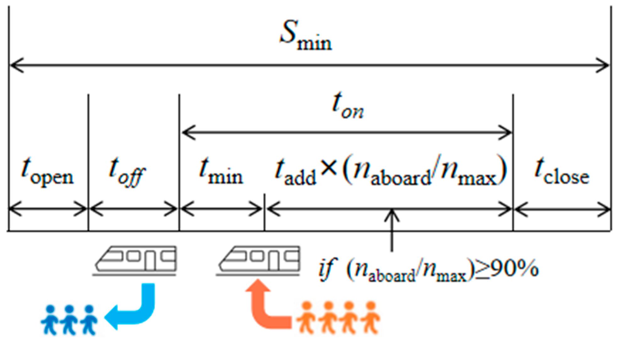
The minimum station dwelling time constraint for trains is defined by Equation (7), where S min represents the minimum station dwelling time. It should be noted that the constraint is applicable only to physical stations. This time is determined based on factors such as the train door opening and closing times, and passenger boarding and alighting times, as expressed in Equation (8). Figure 5 provides a visual representation of the construction of the minimum station dwelling time. In metro systems, the door opening and closing time of the train are usually constant values. The passenger boarding time, on the other hand, is determined by the passenger demand on the platforms. If the number of passengers exceeds 90% of the station’s capacity, the passenger boarding time is increased accordingly [48]. Otherwise, it remains at the minimum passenger boarding time, as depicted in Equation (9).
G ¯ k , i d e p G ¯ k , i a r r S min , k K , i I
S min = t open + t close + t on + t off
t on = t min + t add × n aboard ÷ n max i f n aboard ÷ n max 90 % t min i f n aboard ÷ n max < 90 %
4.
Turnaround Time Constraint
The turnaround time for trains at terminal stations is defined in Equation (10).
G ¯ k , | I | + 1 a r r G ¯ k , | I | d e p T turn min , k K

4. TTR Using Reinforcement Learning

4.1. Improved Q-Learning Algorithm

The Q-learning algorithm is a reinforcement learning algorithm utilized for decision-making in a dynamic environment [49]. It involves iteratively interacting with the environment and adjusting decisions based on trial and error. The objective is to discover the optimal strategy that maximizes cumulative rewards for a given state and action. Traditional Q-learning methods have certain drawbacks, such as dealing with a large state space, difficulties in defining states precisely, and a lack of clear operational steps. Existing research often involves complex state constructions, which can result in inefficient problem-solving. Moreover, these methods may not adequately consider all the factors that contribute to train delays, thereby affecting the real-time responsiveness and prediction accuracy. For real-time train schedule adjustments, we employ an improved Q-learning algorithm, offering the following advantages.
(1)
The Q-learning algorithm offers a concise description and representation of actual states by utilizing a limited set of variables. The usage of limited variables makes the algorithm more practical, reducing the complexity of the state space.
(2)
Pre-training the Q-value state table for various scenarios facilitates quick retrieval during delays or emergencies, enabling a real-time and dynamic selection of strategies such as detaining specific trains or modifying running time. This efficient table lookup and reusability enables our algorithm to make accurate and rapid adjustments in the dynamically changing train operation environment, ensuring both system efficiency and safety.
(3)
The incorporation of a simulated annealing dynamic factor enhances the algorithm’s convergence stability and computational speed. This enables the algorithm to achieve the optimal strategy within a relatively small number of training iterations [50].

4.2. State Definition

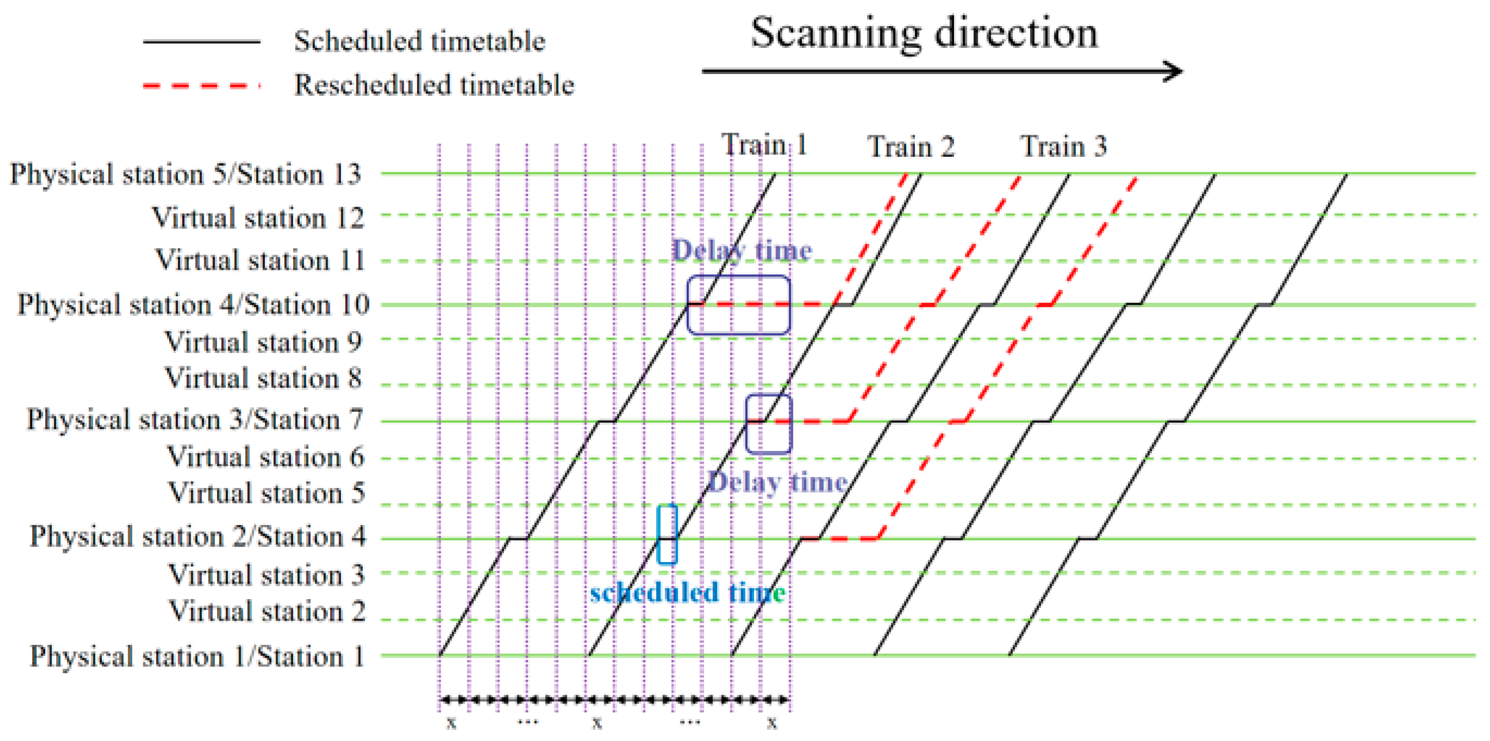
Figure 6 provides an illustration of the state definition utilized in this study, which involves periodically examining whether train arrivals or departures at physical stations are affected by delays. When trains adhere to the scheduled timetable, the situation is similar to that of physical station 2/3 of Train 1 in Figure 6. However, in the case of a delay, the situation of trains would align with physical station 4 of Train 1, and physical station 3 of Train 2. The state ( S ) is represented as a vector, where the length of the vector is determined by the number of physical stations. Each element of the vector S i ( k ) represents the status of the nearest train k arrival at station i , as shown in Equation (11). The determination of the nearest train k can be achieved using the operator k = arg min k G t i m e G k , i a r r ¯ , where arg min k f ( k ) represents taking the value of k that minimizes the function f ( k ) .
The state value is defined by Equations (11) and (12), where G t i m e represents the current checking time.
S = S i ( k ) = D k , i d e l a y ,           k = arg min k G t i m e G k , i a r r ¯ , i I
D k , i d e l a y = 0 i f G ¯ k , i d e p = G k , i d e p D k , i d e l a y = G ¯ k , i d e p G k , i d e p i f G ¯ k , i d e p G t i m e & G ¯ k , i d e p G k , i d e p D k , i d e l a y = G t i m e G k , i d e p i f G ¯ k , i d e p > G t i m e & G ¯ k , i d e p G k , i d e p , i I

4.3. Action

In this paper, the actions are defined as the actual operational strategies. When trains encounter delays, they have the option to choose from three action strategies, as described below:
(1)
Strategy A corresponds to the normal state, where no action for trains is taken.
(2)
Strategy B represents the train movement, where the train chooses a block running time level λ k , i m upon entering the block. The operator arg max m f ( m ) represents taking the value of k that maximises the function f ( k ) .
(3)
Strategy C involves train detention, where the train should determine the duration of detention G k , i a d d in the station before its departure. The duration can be a negative value.
These strategies are depicted in Equations (13) and (14).
a i ( k ) 0 , arg max m λ k , i m , G k , i a d d , i I
G k , i a d d = ( G ¯ k , i d e p G ¯ k , i a r r ) ( G k , i d e p G k , i a r r ) , i I

4.4. Reward Function

The reward in the model is set to assess the matching between the scheduled and actual train timetable. There are two cases for identifying train stop delays. The first case occurs when the train has not arrived at the station by the scheduled departure time or has not resolved the delay and needs to stop at the physical station, as illustrated by physical stations 2 and 3 in Figure 6. The reward for this situation is calculated as the difference between the current checking time and the scheduled departure time of the train, as expressed in Equation (15).
R S i ( k ) , a i ( k ) = G t i m e G k , i d e p , i I
Another scenario is when the delay issue has been resolved and the delayed train has departed, as depicted by physical station 4 in Figure 6. The reward for this situation is calculated as the difference between the actual departure time and the scheduled departure time of the train, as shown in Equation (16).
R S i ( k ) , a i ( k ) = G ¯ k , i d e p G k , i d e p , i I
After calculating the rewards, importance sampling techniques from off-policy learning are employed to update rewards and flexibly utilize experiences from different policies. Taking strategy B as an example, the importance sampling ratio under strategy B can be expressed as shown in Equation (17), where A(s), B(s), and C(s) represent the probabilities of taking actions under policies A, B, and C, respectively, in state s.
Ω = P A s | s P B s | s · P C s | s , A ( s ) P C s | s , B ( s )
According to importance sampling, it is necessary to update the weights via multiplying the reward by the importance sampling ratio Ω. When updating the reward for strategy B, the reward update calculation can be expressed using Equation (18):
R S i ( k ) , a i ( k ) R S i ( k ) , a i ( k ) × Ω
By utilizing the adjusted reward values to update the reward value for strategy B, experiences from strategies A and C are incorporated. The weight adjustments, taking into account the importance sampling ratio, are considered in this process. A similar approach can be applied when updating the reward value for strategies A and C.

4.5. Algorithm Process

An improved Q-learning algorithm is designed to solve the TTR problem and is tailored to real operational scenarios. A matrix is constructed to represent the Q-value state table, as shown in Table 3. The columns represent different states, i.e., all physical stations arranged in the order of operation, while the rows represent all available actions.
The ε-greedy strategy is a commonly used action selection strategy for Q-value state, where the agent explores new actions with a probability of ε and exploits the best action with a probability of (1 − ε). However, excessive exploration in the later stages may affect the convergence speed. To address the balance between exploration and exploitation, the simulated annealing concept is employed to improve the convergence. A temperature parameter is applied to control the degree of exploration. As the iterations progress, the temperature is reduced to decrease the acceptance probability of inferior actions, making it more inclined to exploit advantageous actions. By gradually lowering the temperature, the acceptance probability of suboptimal solutions is reduced, achieving a balance between exploration and exploitation. This accelerates the convergence speed and avoids excessive exploration.
When incorporating the concept of simulated annealing into the Q-learning algorithm, the Metropolis criterion is employed to dynamically regulate the trade-off between exploration and exploitation. The essence of the Metropolis criterion lies in controlling the acceptance probability of new actions through the dynamic adjustment of the temperature parameter. The algorithm follows the following steps:
(1)
Set the optimal action as the current action a i b e s t ( k ) .
(2)
Select an action a i r a n d o m ( k ) randomly.
(3)
A random number δ is generated. According to the Metropolis criterion, the random number δ is compared with o = exp Q S i ( k ) , a i r a n d o m ( k ) Q S i ( k ) , a i b e s t ( k ) / p T to decide whether to accept the new action. If δ is larger, accept the action a k , i r a n d o m as the current action; otherwise, keep the optimal action a i b e s t ( k ) unchanged. Here, p is the adjusting factor, and T represents the number of iterations in the algorithm, both equivalent to the temperature control parameter in the simulated annealing algorithm.
It is obvious that with the increase in T , the value of p T also increases, reducing the probability of accepting inferior actions. This strategy ensures that as the algorithm iterates, the probability of exploration gradually decreases, relying more on the knowledge already learned, thus finding a balance between exploration and exploitation. This strategy can be considered as an equivalent form of the greedy strategy. The adjusting factor p directly influences the rate of temperature reduction. The larger p is, the faster the transition to the greedy strategy.
Once an action is selected, the value of the state–action pair is updated at the corresponding position in the Q-value table according to the state transition probability, as shown in Equation (19). Through continuously performing state transitions and updating the Q-value function, the Q-learning algorithm gradually converges to the optimal Q-value function, thereby learning the optimal action strategy.
Q S i k , a i k Q S i k , a i k + α R S i k , a i k + γ × max a Q S i k , a i k S i k , a i k
where α represents the learning rate, and γ is the discount factor, which can be understood as the importance of future steps. The complete summary of the algorithm process is explained in Algorithm 1.
Algorithm 1: Real-time TTR Algorithm based on improved Q-learning with Train Delays
Step 1. Input the basic information of the transit line, including the planned train timetable and parameters.
Step 2. Input the delay conditions, determine the number of training iterations
Step 3. Set current checking time G time and define the checking time interval, increase the checking time by one interval at each iteration.
  Step 3.1. Perform a sequential check of all stations along the line to determine the state using Equations (11) and (12).
  Step 3.2. For trains that require action, search the Q-value table to identify all potential candidate actions based on the constraint conditions outlined in Equations (2)–(10).
    Step 3.2.1. Calculate the reward value for each candidate action using Equations (15)–(17).
    Step 3.2.2. Select the action to be taken based on the simulated annealing concept.
  Step 3.3. Update the Q-value table using Equation (19).
Step 4. Repeat the above steps (Step 3) until the desired number of model training iterations is achieved.
Step 5. Output the optimal reschedule timetable.

5. Case Study

5.1. Data Input

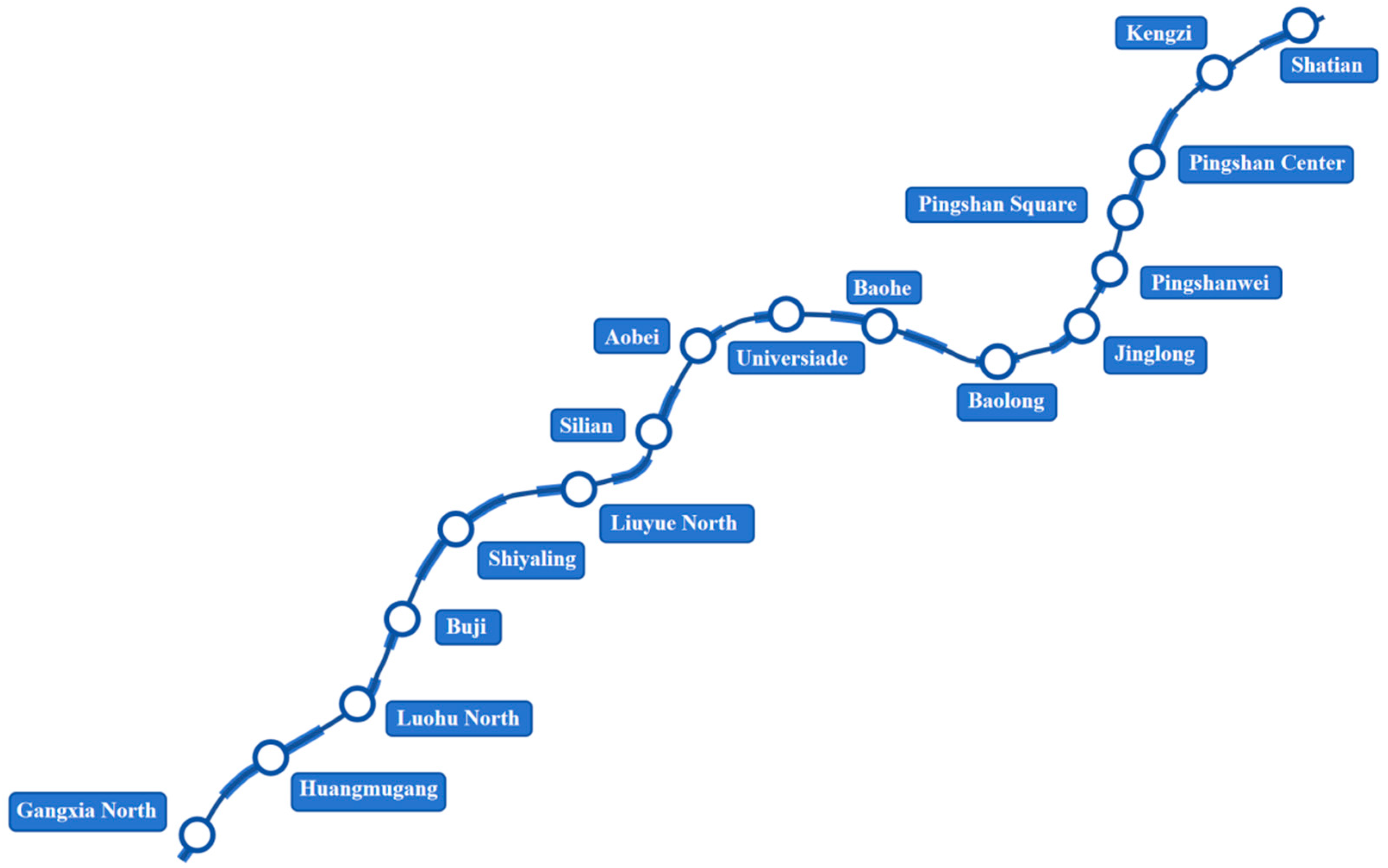
To assess the effectiveness and efficiency of the algorithm, this study selects Shenzhen Metro Line 14 as a case study, as illustrated in Figure 7. The experimental scenario in this research involves the operation of 16 trains, with a total of 17 physical stations along the metro line. The train headway, representing the time interval between consecutive trains, is set to 257 s. Additionally, all trains are assigned the same block running time level in all sections, ensuring uniformity in their travel durations. Furthermore, each train adheres to the scheduled station dwelling time, maintaining consistency in the time spent at each station. The data used in the case study can be found in Supplementary Materials.
The testing period spans from 7:00 AM to 10:00 AM. This timeframe is selected based on Figure 8, which illustrates a substantial passenger flow during the morning peak hours. It is during this period that train headways are relatively short, meaning that delays occurring within this timeframe will have a significant impact on train operations.

5.2. Case Results

The experimental parameters are as follows: learning rate α = 0.02; discount factor γ = 0.8; and adjustment factor p = 0.02. The modeling process is implemented using Python 3.9 on a computer equipped with an Intel(R) Core(TM) i7-9700 CPU at 3.00 GHz. After calculation, the rescheduled train timetable that meets safety requirements and the objective function can be directly output, along with the Q-value table and visualization of the actual train diagram.
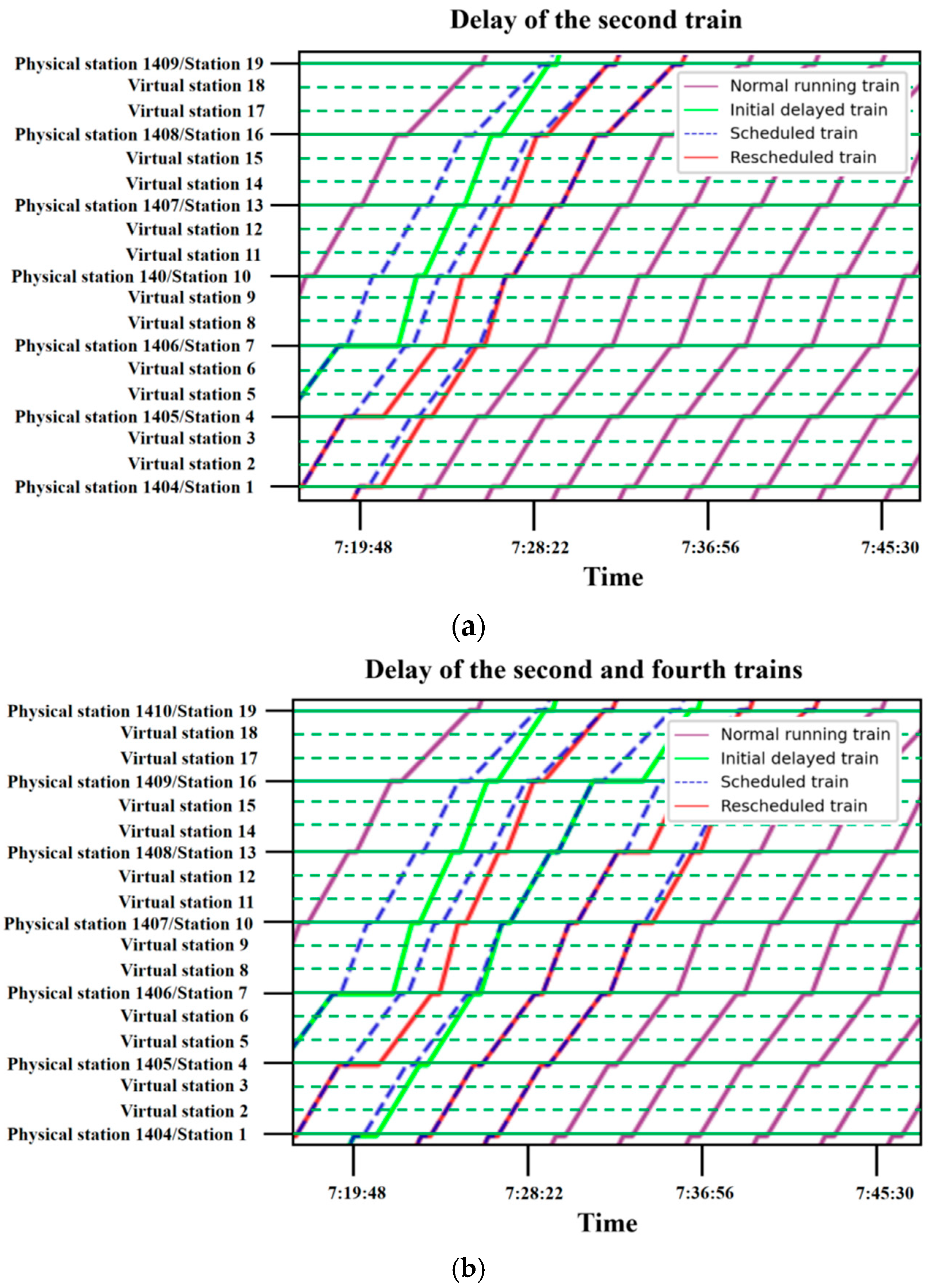
In this case study, two scenarios of train delays are simulated. The first scenario involves a short-term delay of 200 s for one train. Specifically, it is the second train passing through the sixth physical station in the upstream direction, as depicted in Figure 9a. In the figure, the green line represents the train with the initial delay, while the red line represents subsequently affected trains that have been rescheduled. The blue dashed line represents the scheduled timetable, and the purple line represents normally operating trains. As seen in Figure 9a, the number of disrupted trains is minimal, and normal operational order can be quickly restored. Additionally, the subsequent trains experience only a short delay. This rescheduling process ensures safe operation while achieving the minimum sum of deviations between the adjusted actual train operation timetable and the scheduled train operation timetable, which serves as the objective.
In the case of a 200 s delay combined with a 230 s stop time at the sixth physical station, which is close to the 257 s running interval, such short-term delays can usually be smoothly and safely resolved. Standard procedures typically involve detaining trains at subsequent physical stations to ensure safe operation. Delays less than 200 s can also be resolved through adjustments to the train timetable.
The second scenario involves addressing the problem of adjusting the train timetable when multiple delays occur simultaneously, as illustrated in Figure 9b. In this scenario, the second train, operating in the upstream direction, experiences a delay of 200 s when passing through the sixth physical station. Additionally, the fourth train, operating in the upstream direction, encounters a delay of 150 s when passing through the ninth physical station. The delay of the second train has a cascading effect on subsequent trains, resulting in the fourth train experiencing its own delay due to the influence of the initial delay. As depicted in Figure 9b, the algorithm effectively addresses the situation where multiple trains encounter delays at different physical stations, enabling the rapid restoration of normal operational order. Moreover, only a few subsequent trains are affected by these delays. It can be seen that the algorithm successfully reschedules the train timetable when delays between two trains mutually influence each other. This capability proves valuable in resolving train timetable adjustments caused by delays and the mutual influences among multiple trains. By ensuring safety and feasibility in adjusting the train timetable, the algorithm demonstrates its ability to handle and resolve challenges arising from delays and the mutual influences among multiple trains.
Figure 10a,b present partially enlarged train diagrams in combination with the schematic of the blocks for the two scenarios discussed, visually illustrating how the algorithm dynamically adjusts the train timetable. As observed in the figures, trains continue to run through these virtual stations without making any stops. By adjusting the dwelling time of trains at the physical stations and choosing the appropriate section running time for each block, it achieves the objective of minimizing delays while adhering to operational constraints. This optimization methodology significantly improves train punctuality, resulting in a smoother and more efficient travel experience for passengers.

5.3. Results Analysis

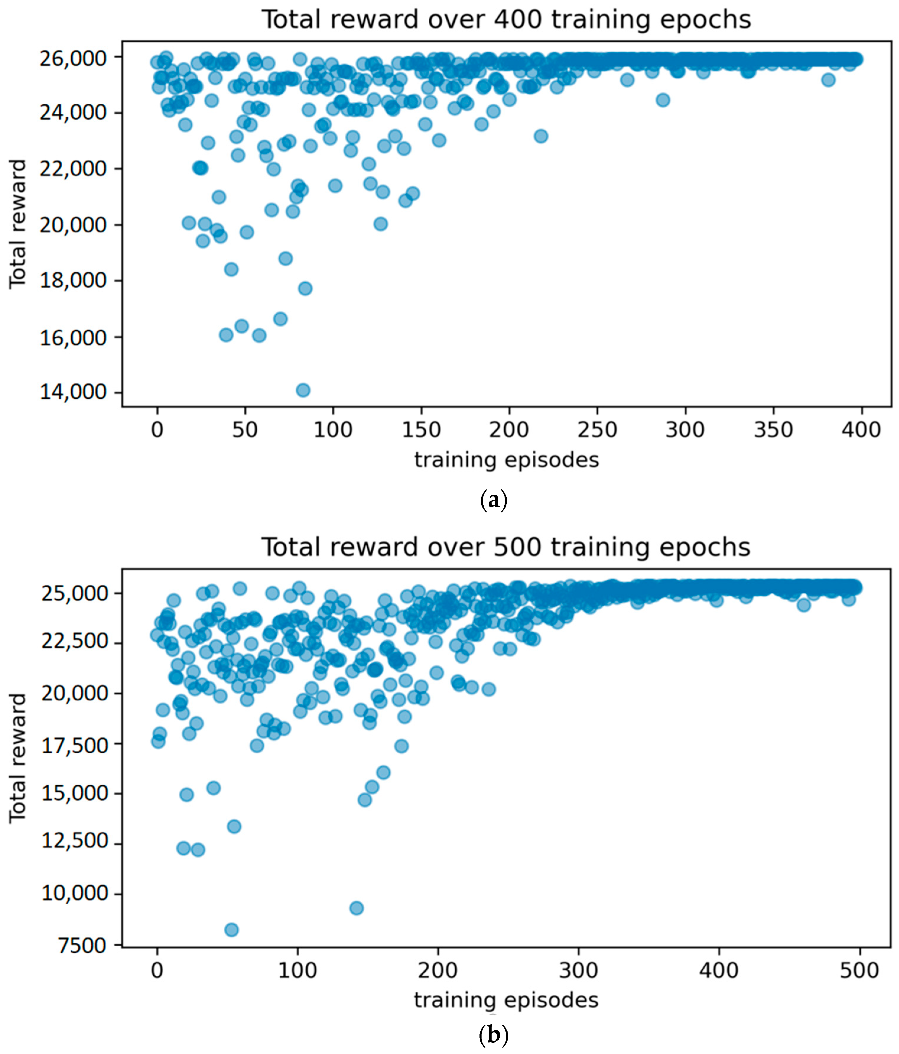
The evaluation of the algorithm’s performance is depicted in Figure 11a,b, which illustrate the total rewards achieved after 400 and 500 iterations, respectively. In the first scenario, convergence is observed after approximately 200 iterations, while in the second scenario, convergence is achieved after around 300 iterations. These results demonstrate the algorithm’s ability to rapidly converge and maintain high stability once convergence is reached. Such characteristics highlight the algorithm’s robustness and fast convergence properties.
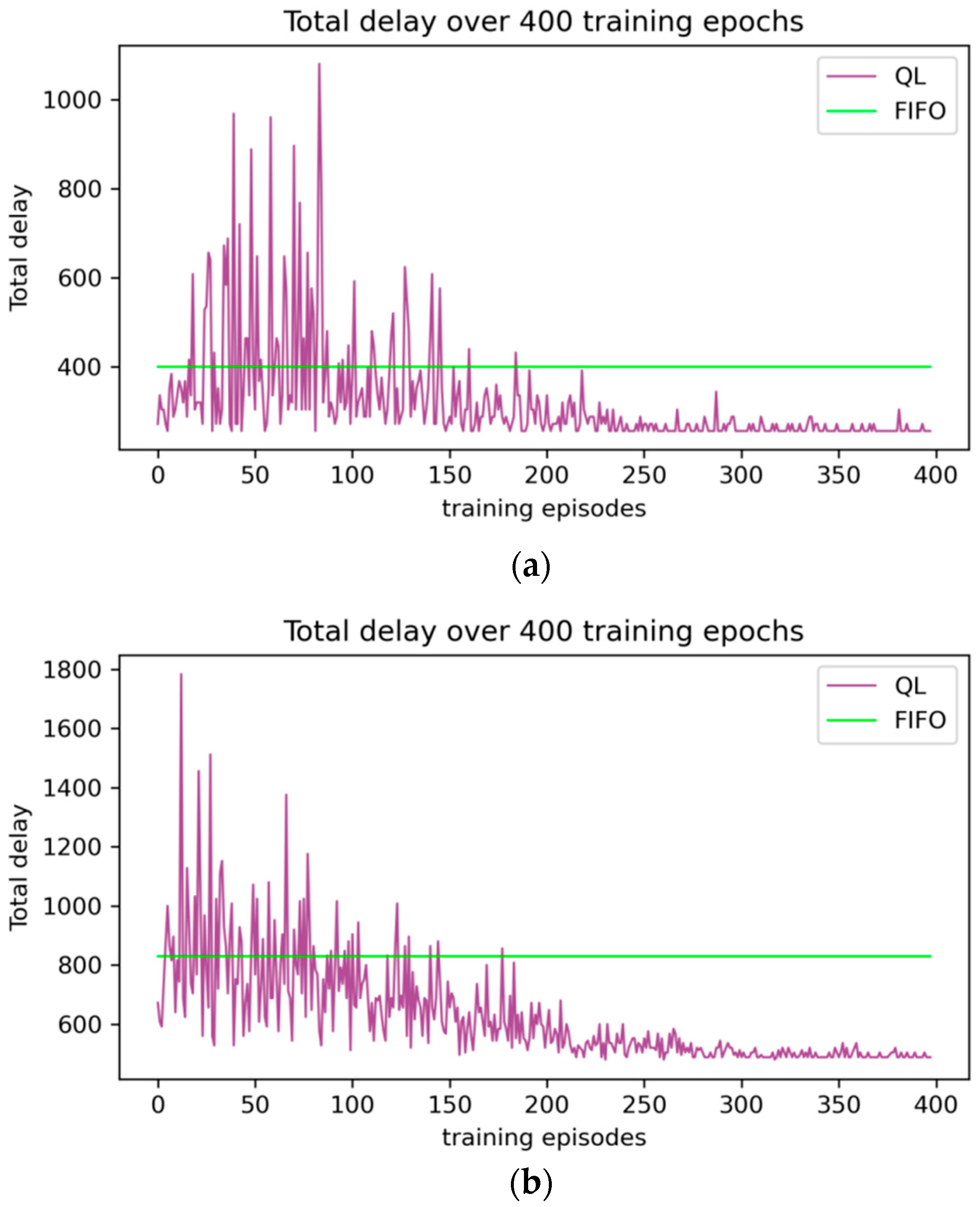
The study compares the total delay values obtained from the proposed algorithm with those of the FIFO algorithm, as depicted in Figure 12a,b. In the first scenario, after approximately 200 iterations, the total delay value obtained from the proposed algorithm is notably lower than that of the FIFO algorithm. Similarly, in the second delay scenario, the proposed algorithm outperforms the FIFO algorithm in less than 250 iterations, again leading to lower total delay values. The limitations of the FIFO algorithm become apparent when faced with multiple delayed trains. In contrast, the proposed algorithm’s ability to dynamically adjust the train timetable and consider operational constraints allows it to effectively minimize delays and achieve superior performance.
To further analyze the advantages of the algorithm proposed in this paper, a comparative analysis was conducted among five approaches: no adjustments, manual adjustment, FIFO, traditional Q-learning, and the improved Q-learning proposed in this study, as shown in Table 4. In the first delay scenario, the number of affected trains for each approach was as follows: 5, 5, 3, 2, and 2, respectively. Regarding the total delay time, the proposed algorithm reduces it from 885 to 256, approximately 71% compared to no adjustments, from 400 to 256, approximately 36% compared to the FIFO algorithm, and from 510 to 256, approximately 49.8% compared to the manual adjustment method. In the second scenario, the number of affected trains for each approach was as follows: 10, 11, 6, 4, and 4, respectively. Regarding the total delay time, the reductions are approximately 72.57% (1750 to 480) compared to no adjustments, approximately 42.17% (830 to 480) compared to the FIFO algorithm, and approximately 50.52% (970 to 480) compared to the manual adjustment method.
Furthermore, compared to the traditional Q-learning algorithm utilizing the ε-greedy strategy (ε = 0.6), the improved algorithm demonstrates notable improvements. In both delay scenarios, the average computation time decreases by approximately 56% and 55.77%, while the average convergence iterations decrease by approximately 62.93% and 67.5%, respectively.

5.4. Sensitivity Analysis

Table 5 provides a comparison of the total delay time for different adjustment factors ( p ) in the two delay scenarios, along with the traditional Q-learning algorithm’s reordering of train schedules. Additionally, the average convergence iteration over multiple experiments is considered. It reveals that when the adjustment factor ( p ) is set to 0.002, the algorithm effectively identifies the optimal train schedule. As the value of p increases, the convergence speed of the algorithm also increases. However, it is important to note that excessively large values of p may cause the algorithm to quickly enter the later stages of greedy selection, potentially resulting in convergence to a local optimum. Consequently, it is crucial to select the adjustment factor appropriately based on the specific circumstances to accelerate the convergence speed of the algorithm without compromising accuracy.
Compared to the traditional ε-greedy strategy of the Q-learning algorithm, the proposed method demonstrates favorable outcomes. The traditional algorithm requires a larger ε value during the exploration process, which leads to a slower convergence speed. In contrast, the proposed method achieves good results by selecting a more suitable adjustment factor, enabling a faster convergence while maintaining accuracy.

5.5. Analysis of Testing on Different Lines

To verify the transferability of the proposed algorithm in this paper, a test was conducted on Shenzhen Metro Line 1. The line involved the operation of 16 trains across 30 stations, with the sections between stations constructed based on the actual layout of the line. The train headway was set at 340 s. In Scenario 1, as depicted in Figure 13a, the 2nd train encountered a delay of 300 s at the 19th physical station. In Scenario 2, illustrated in Figure 13b, the 9th train experienced a 300 s delay at the 18th physical station, and the 11th train faced a 200 s delay at the 16th physical station. In both scenarios, the algorithm demonstrated the capability to swiftly restore normal operation. This case confirms that the proposed algorithm can effectively handle delays and recover the system’s functionality across different metro lines.

6. Conclusions

In this study, an optimization model is established, and an improved Q-learning algorithm is proposed to address the TTR problem. The Shenzhen Metro is used as a case study, and the results demonstrate that satisfactory solutions can be achieved within a short time. The proposed approach effectively meets the real-time timetable adjustment requirements, showcasing its ability to quickly reschedule train timetables in response to actual metro operation delays. The main conclusions of this study are as follows:
(1)
The improved Q-learning algorithm exhibited a stable convergence and rapid computation speed. Compared to no adjustment, manual adjustment, and FIFO methods, it achieved average reductions of approximately 39.09%, 50.16%, and 71.82% in total train delay, respectively. In comparison to the traditional Q-learning algorithm, the average computation time decreased by around 55.89%, and the average iteration count decreased by approximately 65.22%.
(2)
The optimized method resulted in a more evenly rescheduled train timetable and aimed to minimize the total delay time caused by train delays. It effectively coordinated the detention of subsequent trains and the adjustment of section running times, ensuring the smooth operation of subsequent trains.
(3)
The transferability of the algorithm proposed in this paper is verified through the case study of Shenzhen Metro Line 1. This method demonstrates real-time adjustment capability and promotes the utilization of pre-trained Q-value table in various scenarios.
In our future research, we will conduct experimental analyses on different metro systems to enhance the robustness and generalizability of the proposed algorithm. Additionally, we will explore the incorporation of more complex state variables to further improve the accuracy of our model. To address the challenge of dealing with large-scale state variables, we will consider utilizing deep reinforcement learning algorithms, such as deep Q-networks (DQN).

Supplementary Materials

The following supporting information can be downloaded at: https://www.mdpi.com/article/10.3390/app14041552/s1.

Author Contributions

The authors confirm contribution to the paper as follows: study conception and design, data collection, analysis and interpretation of results, draft manuscript preparation: Y.H.; study conception and design, analysis and interpretation of results, funding acquisition: W.L. and Q.L. All authors have read and agreed to the published version of the manuscript.

Funding

This paper is supported by the National Social Science Fund of China (20BGL301).

Institutional Review Board Statement

Not applicable.

Informed Consent Statement

Not applicable.

Data Availability Statement

The data presented in this study are available in the article and Supplementary Materials.

Conflicts of Interest

The authors declare no conflicts of interest.

References

  1. Latif, K.; Sharafat, A.; Seo, J. Digital Twin-Driven Framework for TBM Performance Prediction, Visualization, and Monitoring through Machine Learning. Appl. Sci. 2023, 13, 11435. [Google Scholar] [CrossRef]
  2. Melo, P.C.; Harris, N.G.; Graham, D.J.; Anderson, R.J.; Barron, A. Determinants of delay incident occurrence in urban metros. Transp. Res. Rec. 2011, 2216, 10–18. [Google Scholar] [CrossRef]
  3. Li, W.; Peng, Q.; Wen, C.; Wang, P.; Lessan, J.; Xu, X. Joint optimization of delay-recovery and energy-saving in a metro system: A case study from China. Energy 2020, 202, 117699. [Google Scholar] [CrossRef]
  4. Zhou, P.; Chen, L.; Dai, X.; Li, B.; Chai, T. Intelligent prediction of train delay changes and propagation using RVFLNs with improved transfer learning and ensemble learning. IEEE Trans. Intell. Transp. Syst. 2020, 22, 7432–7444. [Google Scholar] [CrossRef]
  5. Cacchiani, V.; Huisman, D.; Kidd, M.; Kroon, L.; Toth, P.; Veelenturf, L.; Wagenaar, J. An overview of recovery models and algorithms for real-time railway rescheduling. Transp. Res. Part B Methodol. 2014, 63, 15–37. [Google Scholar] [CrossRef]
  6. Cheng, R.; Song, Y.; Chen, D.; Chen, L. Intelligent localization of a high-speed train using LSSVM and the online sparse optimization approach. IEEE Trans. Intell. Transp. Syst. 2017, 18, 2071–2084. [Google Scholar] [CrossRef]
  7. Pellegrini, P.; Marlière, G.; Pesenti, R.; Rodriguez, J. RECIFE-MILP: An effective MILP-based heuristic for the real-time railway traffic management problem. IEEE Trans. Intell. Transp. Syst. 2015, 16, 2609–2619. [Google Scholar] [CrossRef]
  8. Lamorgese, L.; Mannino, C. An exact decomposition approach for the real-time train dispatching problem. Oper. Res. 2015, 63, 48–64. [Google Scholar] [CrossRef]
  9. Yue, P.; Jin, Y.; Dai, X.; Feng, Z.; Cui, D. Reinforcement learning for online dispatching policy in real-time train timetable rescheduling. IEEE Trans. Intell. Transp. Syst. 2023, 25, 478–490. [Google Scholar] [CrossRef]
  10. Wang, P.; Ma, L.; Goverde RM, P.; Wang, Q. Rescheduling trains using Petri nets and heuristic search. IEEE Trans. Intell. Transp. Syst. 2015, 17, 726–735. [Google Scholar] [CrossRef]
  11. Fang, W.; Yang, S.; Yao, X. A survey on problem models and solution approaches to rescheduling in railway networks. IEEE Trans. Intell. Transp. Syst. 2015, 16, 2997–3016. [Google Scholar] [CrossRef]
  12. Walraevens, J.; Bruneel, H.; Fiems, D.; Wittevrongel, S. Delay analysis of multiclass queues with correlated train arrivals and a hybrid priority/FIFO scheduling discipline. Appl. Math. Model. 2017, 45, 823–839. [Google Scholar] [CrossRef]
  13. Zhang, C.; Gao, Y.; Yang, L.; Gao, Z.; Qi, J. Joint optimization of train scheduling and maintenance planning in a railway network: A heuristic algorithm using Lagrangian relaxation. Transp. Res. Part B Methodol. 2020, 134, 64–92. [Google Scholar] [CrossRef]
  14. Zhu, Y.; Goverde, R.M.P. Dynamic railway timetable rescheduling for multiple connected disruptions. Transp. Res. Part C Emerg. Technol. 2021, 125, 103080. [Google Scholar] [CrossRef]
  15. Pellegrini, P.; Marlière, G.; Rodriguez, J. Optimal train routing and scheduling for managing traffic perturbations in complex junctions. Transp. Res. Part B Methodol. 2014, 59, 58–80. [Google Scholar] [CrossRef]
  16. Kersbergen, B.; van den Boom, T.; De Schutter, B. Distributed model predictive control for railway traffic management. Transp. Res. Part C Emerg. Technol. 2016, 68, 462–489. [Google Scholar] [CrossRef]
  17. D’ariano, A.; Pacciarelli, D.; Pranzo, M. A branch and bound algorithm for scheduling trains in a railway network. Eur. J. Oper. Res. 2007, 183, 643–657. [Google Scholar] [CrossRef]
  18. Min, Y.H.; Park, M.J.; Hong, S.P.; Hong, S.H. An appraisal of a column-generation-based algorithm for centralized train-conflict resolution on a metropolitan railway network. Transp. Res. Part B Methodol. 2011, 45, 409–429. [Google Scholar] [CrossRef]
  19. Zhan, S.; Wong, S.C.; Shang, P.; Peng, Q.; Xie, J.; Lo, S.M. Integrated railway timetable rescheduling and dynamic passenger routing during a complete blockage. Transp. Res. Part B Methodol. 2021, 143, 86–123. [Google Scholar] [CrossRef]
  20. Zhou, L.; Tong, L.C.; Chen, J.; Tang, J.; Zhou, X. Joint optimization of high-speed train timetables and speed profiles: A unified modeling approach using space-time-speed grid networks. Transp. Res. Part B Methodol. 2017, 97, 157–181. [Google Scholar] [CrossRef]
  21. Peng, S.; Yang, X.; Ding, S.; Wu, J.; Sun, H. A dynamic rescheduling and speed management approach for high-speed trains with uncertain time-delay. Inf. Sci. 2023, 632, 201–220. [Google Scholar] [CrossRef]
  22. Liu, X.; Zhou, M.; Dong, H.; Wu, X.; Li, Y.; Wang, F.Y. ADMM-based joint rescheduling method for high-speed railway timetabling and platforming in case of uncertain perturbation. Transp. Res. Part C Emerg. Technol. 2023, 152, 104150. [Google Scholar] [CrossRef]
  23. Kumar, N.; Mishra, A. A multi-objective and dictionary-based checking for efficient rescheduling trains. Alex. Eng. J. 2021, 60, 3233–3241. [Google Scholar] [CrossRef]
  24. Wang, R.; Zhang, Q.; Dai, X.; Yuan, Z.; Zhang, T.; Ding, S.; Jin, Y. An efficient evolutionary algorithm for high-speed train rescheduling under a partial station blockage. Appl. Soft Comput. 2023, 145, 110590. [Google Scholar] [CrossRef]
  25. Li, K.P.; Gao, Z.Y. An improved car-following model for railway traffic. J. Adv. Transp. 2013, 47, 475–482. [Google Scholar] [CrossRef]
  26. Corman, F.; Trivella, A.; Keyvan-Ekbatani, M. Stochastic process in railway traffic flow: Models, methods and implications. Transp. Res. Part C Emerg. Technol. 2021, 128, 103167. [Google Scholar] [CrossRef]
  27. Ketphat, N.; Whiteing, A.; Liu, R. State movement for controlling trains operating under the virtual coupling system. Proc. Inst. Mech. Eng. Part F J. Rail Rapid Transit 2022, 236, 172–182. [Google Scholar] [CrossRef]
  28. Liu, Y.; Zhou, Y.; Su, S.; Xun, J.; Tang, T. An analytical optimal control approach for virtually coupled high-speed trains with local and string stability. Transp. Res. Part C Emerg. Technol. 2021, 125, 102886. [Google Scholar] [CrossRef]
  29. Saidi, S.; Koutsopoulos, H.N.; Wilson NH, M.; Zhao, J. Train following model for urban rail transit performance analysis. Transp. Res. Part C Emerg. Technol. 2023, 148, 104037. [Google Scholar] [CrossRef]
  30. Corman, F.; D’Ariano, A.; Pacciarelli, D.; Pranzo, M. A tabu search algorithm for rerouting trains during rail operations. Transp. Res. Part B Methodol. 2010, 44, 175–192. [Google Scholar] [CrossRef]
  31. Zhou, M.; Liu, Y.; Mo, H.; Shang, J.; Dong, H. Timetable Rescheduling for High-Speed Railways under Temporary Segment Blockage based on Genetic Simulated Annealing Algorithm. In Proceedings of the 2022 China Automation Congress (CAC), Xiamen, China, 25–27 November 2022; pp. 6867–6872. [Google Scholar]
  32. He, Z.; Liu, T.; Liu, H. Improved particle swarm optimization algorithms for aerodynamic shape optimization of high-speed train. Adv. Eng. Softw. 2022, 173, 103242. [Google Scholar] [CrossRef]
  33. Eaton, J.; Yang, S. Dynamic railway junction rescheduling using population based ant colony optimisation. In Proceedings of the 2014 14th UK Workshop on Computational Intelligence (UKCI), Bradford, UK, 8–10 September 2014; pp. 1–8. [Google Scholar]
  34. Qu, Q.; Li, X.; Zhou, Y.; Zeng, J.; Yuan, M.; Wang, J.; Lv, J.; Liu, K.; Mao, K. An improved reinforcement learning algorithm for learning to branch. arXiv 2022, arXiv:2201.06213. [Google Scholar]
  35. Tang, Y.; Agrawal, S.; Faenza, Y. Reinforcement learning for integer programming: Learning to cut. In Proceedings of the International Conference on Machine Learning, Vienna, Austria, 13–18 July 2020; pp. 9367–9376. [Google Scholar]
  36. Dündar, S.; Şahin, İ. Train re-scheduling with genetic algorithms and artificial neural networks for single-track railways. Transp. Res. Part C Emerg. Technol. 2013, 27, 1–15. [Google Scholar] [CrossRef]
  37. Šemrov, D.; Marsetič, R.; Žura, M.; Todorovski, L.; Srdic, A. Reinforcement learning approach for train rescheduling on a single-track railway. Transp. Res. Part B Methodol. 2016, 86, 250–267. [Google Scholar] [CrossRef]
  38. Khadilkar, H. A scalable reinforcement learning algorithm for scheduling railway lines. IEEE Trans. Intell. Transp. Syst. 2018, 20, 727–736. [Google Scholar] [CrossRef]
  39. Zhu, Y.; Wang, H.; Goverde, R.M.P. Reinforcement learning in railway timetable rescheduling. In Proceedings of the 2020 IEEE 23rd International Conference on Intelligent Transportation Systems (ITSC), Rhodes, Greece, 20–23 September 2020; p. 9294188. [Google Scholar]
  40. Li, W.; Ni, S. Train timetabling with the general learning environment and multi-agent deep reinforcement learning. Transp. Res. Part B Methodol. 2022, 157, 230–251. [Google Scholar] [CrossRef]
  41. Ning, L.; Li, Y.; Zhou, M.; Song, H.; Dong, H. A deep reinforcement learning approach to high-speed train timetable rescheduling under disturbances. In Proceedings of the 2019 IEEE Intelligent Transportation Systems Conference (ITSC), Auckland, New Zealand, 27–30 October 2019; pp. 3469–3474. [Google Scholar]
  42. Ghasempour, T.; Nicholson, G.L.; Kirkwood, D.; Fujiyama, T.; Heydecker, B. Distributed approximate dynamic control for traffic management of busy railway networks. IEEE Trans. Intell. Transp. Syst. 2019, 21, 3788–3798. [Google Scholar] [CrossRef]
  43. Wang, Y.; Lv, Y.; Zhou, J.; Yuan, Z.; Zhang, Q.; Zhou, M. A policy-based reinforcement learning approach for high-speed railway timetable rescheduling. In Proceedings of the 2021 IEEE International Intelligent Transportation Systems Conference (ITSC), Indianapolis, IN, USA, 19–22 September 2021; pp. 2362–2367. [Google Scholar]
  44. Su, B.; Wang, Z.; Su, S.; Tang, T. Metro train timetable rescheduling based on q-learning approach. In Proceedings of the 2020 IEEE 23rd International Conference on Intelligent Transportation Systems (ITSC), Rhodes, Greece, 20–23 September 2020; pp. 1–6. [Google Scholar]
  45. Liao, J.; Yang, G.; Zhang, S.; Zhang, F.; Gong, C. A deep reinforcement learning approach for the energy-aimed train timetable rescheduling problem under disturbances. IEEE Trans. Transp. Electrif. 2021, 7, 3096–3109. [Google Scholar] [CrossRef]
  46. Ran, X.C.; Chen, S.K.; Liu, G.H.; Bai, Y. Energy-efficient approach combining train speed profile and timetable optimisations for metro operations. IET Intell. Transp. Syst. 2020, 14, 1967–1977. [Google Scholar] [CrossRef]
  47. Zhao, Y.; Ding, X. The Research on Delay Propagation of Urban Rail Transit Operation under Sudden Failure. J. Adv. Transp. 2021, 2021, 8984474. [Google Scholar] [CrossRef]
  48. Liu, R.; Li, S.; Yang, L. Collaborative optimization for metro train scheduling and train connections combined with passenger flow control strategy. Omega 2020, 90, 101990. [Google Scholar] [CrossRef]
  49. Peng, J.; Williams, R.J. Incremental multi-step Q-learning. In Machine Learning Proceedings 1994; Morgan Kaufmann: Burlington, MA, USA, 1994; pp. 226–232. [Google Scholar]
  50. Li, J.; Li, Y.; Su, Q. Sequential recovery of cyber-physical power systems based on improved q-learning. J. Frankl. Inst. 2023, 360, 13692–13711. [Google Scholar] [CrossRef]
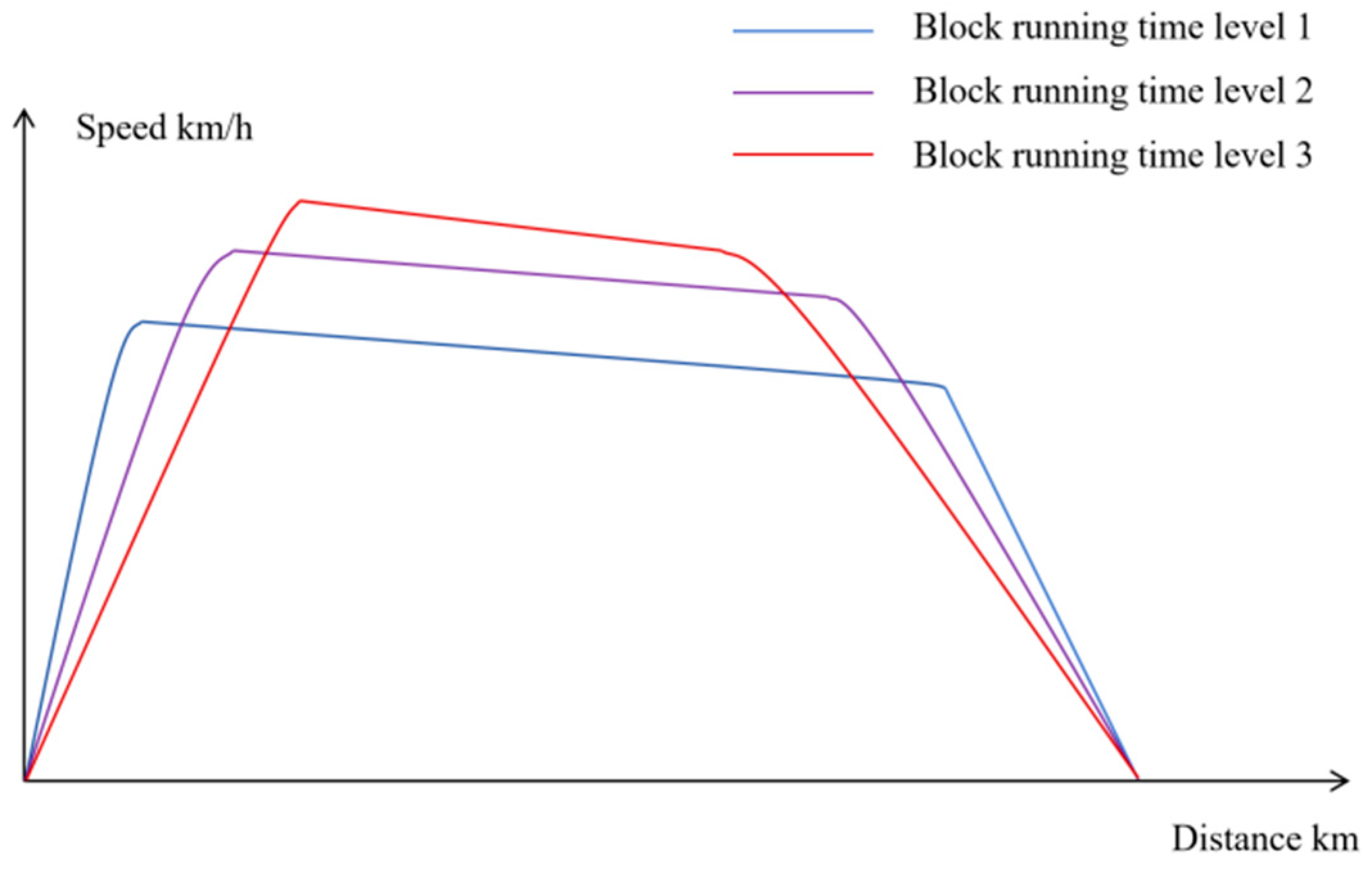
Figure 1. Schematic diagram of different block running time levels.
Applsci 14 01552 g001
Figure 2. Train delay with train dwell and train optimization adjustment.
Applsci 14 01552 g002
Figure 3. Diagram of bi-directional metro line.
Applsci 14 01552 g003
Figure 4. Schematic diagram of train interaction zone under emergency situations.
Applsci 14 01552 g004
Figure 5. Schematic diagram of the construction of station dwelling time.
Applsci 14 01552 g005
Figure 6. State definition with train delays.
Applsci 14 01552 g006
Figure 7. Diagram of Shenzhen Metro Line 14.
Applsci 14 01552 g007
Figure 8. Passenger flow for Shenzhen Metro Line 14 on a weekday.
Applsci 14 01552 g008
Figure 9. Two scenarios of train delays in the case of Shenzhen Metro Line 14. (a) Scenario I: the second train experienced a delay of 200 s at the sixth physical station. (b) Scenario II: the second train experienced a delay of 200 s at the sixth physical station, and the fourth train experienced a delay of 150 s at the ninth physical station.
Applsci 14 01552 g009
Figure 10. Partial train diagrams illustrating delays in the two scenarios of Shenzhen Metro Line 14. (a) Scenario I: the second train experienced a delay of 200 s at the sixth physical station. (b) Scenario II: the second train experienced a delay of 200 s at the sixth physical station, and the fourth train experienced a delay of 150 s at the ninth physical station.
Applsci 14 01552 g010
Figure 11. The total reward value when delays occur in the two scenarios of Shenzhen Metro Line 14. (a) Scenario I: the second train experienced a delay of 200 s at the sixth physical station. (b) Scenario II: the second train experienced a delay of 200 s at the sixth physical station, and the fourth train experienced a delay of 200 s at the ninth physical station.
Applsci 14 01552 g011
Figure 12. The total delay values in the two scenarios on Shenzhen Metro Line 14 when delays occur using Q-learning (QL) and FIFO strategies. (a) Scenario I: the second train experienced a delay of 200 s at the sixth physical station. (b) Scenario II: the second train experienced a delay of 200 s at the sixth physical station, and the fourth train experienced a delay of 200 s at the ninth physical station.
Applsci 14 01552 g012
Figure 13. Two scenarios of train delays in the case of Shenzhen Metro Line 1. (a) Scenario I: the 2nd train experienced a delay of 300 s at the 19th physical station. (b) Scenario II: the 9th train experienced a delay of 300 s at the 18th physical station, and the 11th train experienced a delay of 200 s at the 16th physical station.
Applsci 14 01552 g013
Table 1. Brief summary of the existing learning-based methods in the TTR problem.
WorkProblem SettingTraining InstancesState Definition
Šemrov et al. [37]Multiple train delaysSingle instanceTrain locations, current time
and track availability
Khadilkar et al. [38]Multiple train delaysSingle instanceTrack availability around
the train to be controlled
Zhu et al. [39]Multiple train delaysSingle instanceDelay time, location, and local
track availability of the current train
Li et al. [40]Multiple train delaysSingle instanceDeparture time, whether to stop at stations, and running direction of the current train
Ning et al. [41]Multiple train delaysSingle instanceActual arrival time and
departure time of trains
Ghasempour et al. [42]Single train delaysMultiple instancesArrival and departure time of
trains entering junction
Yin et al. [43]Single train delaysMultiple instancesPlanned/actual arrival time and departure time
Su et al. [44]Single train delaysMultiple instancesActual arrival time and the number of passengers onboard
Liao et al. [45]Single train delaysMultiple instancesThe speed, position, and
current driving status of the train
This paperMultiple train delaysMultiple instancesTrain delays
Table 2. Notations and parameters used in the formulation.
NotationsDefinition
Set
K Set   of   train   services .   K = 1 , 2 , , K .   K is the maximum index of train services
I Set   of   stations ,   including   physical   and   virtual   stations .   I = 1 , 2 , , 2 I .   2 I is the end index of stations.
I Set of physical stations.
M Set   of   block   running   time   levels .   M = 1 , 2 , , M .   M is the maximum index of block running time levels.
k Index   of   train   service ,   k K
i Index   of   station ,   i I
m Index   of   block   running   time   level ,   m M
Input Parameter
G k , i a r r Scheduled arrival time of train service k at physical station i , i I
G k , i d e p Scheduled departure time of train service k at physical station i , i I
λ k , i m The running time of train service k using block running time level m from station i   to   i + 1
μ k , i m The Boolean variable to decide whether block running time level m from station i   to   i + 1 for train service k is selected.
U min Minimum train headway on the truck line
B k The block where train service k locates
S min Minimum station dwelling time on the truck line
t open Time for door opening after train’s arrival
t close Time for door closing before train’s departure
t min Minimum boarding and alighting time for passengers
n max Maximum station passenger capacity
n aboard Number of passengers entering the station
T turn min Minimum turnaround time at the turnaround station
Intermediate variables
G ¯ k , i a r r Rescheduled arrival time of train service k at station i
G ¯ k , i d e p Rescheduled departure time of train service k at station i
t on Boarding time for passengers
t off Alighting time for passengers
t add Additional boarding and alighting time for passengers
D k , i d e l a y Delay time of train service k at physical station i ,   i I
G time Current checking time
G k , i a d d Additional dwelling time of train service k at physical station i ,   i I
a i r a n d o m ( k ) The random action for train service k at physical station i ,   i I
a i b e s t ( k ) The optimal action for train service k at physical station i ,   i I
Table 3. An example of a Q-value state table.
Physical StationsStateAction
Strategy AStrategy BStrategy C/(s)
12−1010
(1401,1402,…,1417)(0,0,…,0)00000
(1401,1402,…,1417)(0,0,…,50,…,0)0003520
(1401,1402,…,1417)(0,0,…,0)20010010
(1401,1402,…,1417)(0,0,…,0)30100400
(1401,1402,…,1417)(0,…,50,…,100,…,0)151001010
Table 4. Comparison of the effectiveness of the proposed algorithm with other methods.
No AdjustmentManual AdjustmentFIFOTraditional Q-Learning
(ε = 0.6)
The Proposed Method
Scenario 1
Total delay time (s)885510400256256
Affected trains55322
Affected physical stations56322
Average computation time (min)85.10.12.51.1
Average Convergence Iterations---634235
Scenario 2
Total delay time (s)1750970830480480
Affected trains1011644
Affected physical stations1312644
Average computation time (min)1612.30.15.22.3
Average Convergence Iterations---763312
Table 5. Optimization results of train schedules with different p or ε values in two delay scenarios.
No.The Proposed MethodTraditional Q-Learning
p = 0.002p = 0.005p = 0.01p = 0.02ε = 0.6ε = 0.4
Delay scenario 1256 (591) *256 (363)256 (251)256 (235)256 (634)256 (661)
Delay scenario 2480 (640)480 (484)480 (334)480 (248)480 (763)480 (782)
* Total delay time (average convergence iterations).
Disclaimer/Publisher’s Note: The statements, opinions and data contained in all publications are solely those of the individual author(s) and contributor(s) and not of MDPI and/or the editor(s). MDPI and/or the editor(s) disclaim responsibility for any injury to people or property resulting from any ideas, methods, instructions or products referred to in the content.