Abstract
With the advancement of sensor technology, distributed processing technology, and wireless communication, Visual Sensor Networks (VSNs) are widely used. However, VSNs also have flaws such as poor data synchronization, limited node resources, and complicated node management. Thus, this paper proposes a sensor placement optimization method to save network resources and facilitate management. First, some necessary models are established, including the sensor model, the space model, the coverage model, and the reconstruction error model, and a dimensionality reduction search method is proposed. Next, following the creation of a multi-objective optimization function to balance reconstruction error and coverage, a clever optimization algorithm that combines the benefits of Genetic Algorithms (GA) and Particle Swarm Optimization (PSO) is applied. Finally, comparison studies validate the methodology presented in this paper, and the combined algorithm can enhance optimization effect while relatively reducing running time. In addition, a sensor coverage method for large-range target space with obstacles is discussed.
1. Introduction
With the rapid development of the Internet of Things (IoT) and 4G/5G networks, Wireless Sensor Networks (WSNs) are widely used in many scenarios due to their high degree of flexibility, fault tolerance, autonomy, and rapid deployment [1,2]. However, the monitoring information of most WSNs is limited to scalar data such as temperature, pressure, vibration, humidity, etc. in the environment, which is, after all, limited and insufficient to support the application of WSNs in more complex scenarios. In contrast, Visual Sensor Networks (VSNs) have the advantages of contactless measurement, rich dimensions of sensory information, and strong anti-interference capability. The VSNs are distributed perception networks that can track targets and achieve wide-area coverage, and they are composed of multiple smart camera nodes. At the moment, VSNs are widely used in surveillance [3,4], object detection [5], indoor patient monitoring [6], autonomous driving [7], smart city [8] and Unmanned Aerial Vehicles [9,10]. But the emergence of VSNs also brings with it a number of difficulties. For instance, there are many nodes dispersed extensively throughout the networks, which makes node administration challenging. Additionally, the resources available to camera nodes, such as processing, storage, and network connection bandwidth, are limited, and data synchronization is subpar. Therefore, while building VSNs, variables like sensor number, location, and orientation, i.e., the sensor placement optimization problem, have a significant impact on coverage and can alter the ability of the sensor networks to identify and monitor objects.
The original sensor placement research is based on the well-known Art Gallery Problem (AGP), which is concerned with determining the smallest number of guards required to cover the inside of an art gallery room [11,12]. By adding some special constraints, AGP can be extended into a sensor placement problem. Thus, the art gallery problem is often regarded as the predecessor of the sensor placement problem [13]. Many variable parameters and constraints need to be considered, such as the location constraints of each sensor, the coverage requirements of a specific area, different types of vision sensors, and different sorts of obstacles. Therefore, this type of problem is more complicated than the traditional AGP.
A number of studies on sensor coverage optimization have been conducted recently. Altahir et al. [14] tackle the camera placement problem based on an inverse modeling taxonomy. Kelp et al. [15] suggest a pilot project that uses multiresolution dynamic mode decomposition to determine where PM2.5 sensors should be placed for the best results. In order to address the optimal camera placement problem, Chebi [16] suggests a technique based on the Dragonfly Algorithm, which is motivated by the motion and behaviors of artificial objects in the environment. With the use of high-resolution 3D grids as a model, Puligandla et al. [17] present a multi-resolution technique that makes it possible to apply current optimization algorithms to expansive real-world issues. Ali et al. [18] propose a camera placement method to ensure extensive coverage while maintaining high-quality images and minimizing overlap between cameras. Zhang et al. [19] introduce a novel field-of-view model resembling the human eye. They solve the optimization problem of visual sensor placement using a nonlinear programming algorithm.
There are two main types of representative discrete optimization algorithms: integer programming and heuristics algorithms. When some or all of the optimization variables are restricted to pure integers, it can be abstracted as an integer programming problem. And if part of the variables are not restricted to integers, this becomes a Mixed Integer Programming (MIP) problem [20]. The binary programming problem is a special case of the integer programming problem [21,22], in which variables are limited to zero or one. Such a binary problem is common in sensor placement applications. However, there is also a more realistic probabilistic sensing model in which the coverage in the sensor’s sensing range is described as a probability function [23]. Each point in the space is assigned a probability, indicating the probability for the point to be covered. Sometimes, some variables in the layout problem are binary (such as whether or not the camera is placed), and some variables are integers (such as the number of cameras). This kind of problem can be treated as an MIP problem. There is also a large class of discrete optimization algorithms called heuristic algorithms, which are usually used in combinatorial optimization. Although these algorithms cannot guarantee optimal solutions, they can produce a satisfactory outcome within reasonable time. Heuristic algorithms include Simulated Annealing (SA) [24], Genetic Algorithm (GA) [25,26], Particle Swarm Optimization (PSO) [27,28] and so on.
The current literature on sensor coverage rarely considers both reconstruction error and coverage; instead, the majority of studies concentrate on the 1-coverage problem for a target point, which states that it is sufficient to require that the object point be covered by a single sensor. However, in practical applications, it is sometimes necessary to make the target area covered by multiple sensors. For reconstruction of spatial points by multi-camera systems, it is usually required that the spatial points are captured by multiple cameras at the same time, i.e., the requirement of at least two coverage points must be satisfied. By striking a balance between coverage and reconstruction error, the system is able to capture scene information and provide high-quality reconstruction. Therefore, in this paper, we consider the reconstruction error constraints of the visual tracking task and comprehensively consider the compromise balance of maximizing coverage and minimizing reconstruction error as the objective function. The significant contributions of this paper are as follows:
- Detailed mathematical models of the sensor placement optimization problem are built.
- A search approach for dimensionality reduction is proposed.
- A multi-objective optimization function is proposed that considers reconstruction error in addition to coverage.
- A combination of PSO and GA algorithms is used to avoid the local optima while increasing optimization speed.
- A sensor coverage method for large-range target space with obstacles is discussed.
The rest of the paper is structured as follows: in Section 2, we provide a mathematical formulation about the sensor placement problem and also a few basic models, including sensor model, space model, coverage model, and reconstruction error model and propose a dimensionality reduction search method. Next, in Section 3, a multi-objective optimization function is established to consider the space coverage and reconstruction error for 2D spaces, followed by a suitable multi-objective optimization algorithm. In Section 4, extensive comparison experiments are carried out to evaluate the given camera position optimization algorithms. Finally, Section 5 summarizes the conclusions and proposes plans for future research.
2. Problem Formulation
The sensor placement optimization of VSNs is a practical engineering problem which aims to determine the optimal deployment of sensors in the actual physical space. During the research process, it is necessary to abstract the real camera and physical space as mathematical models for quantitative analysis purposes. In this section, the problem is first described as mathematical optimization with some necessary assumptions. Then, we establish some fundamental models as the mathematical foundation of the optimization process, including the sensor model, the space model, the coverage model, and the reconstruction error model, and propose a dimensionality reduction search method.
2.1. Problem Statement
The main objective of this proposal is to determine the optimal deployment of the sensors in the actual physical space. First, we make the assumption that the camera type and parameters are the same, i.e., that the unified camera perception model is used. Subsequently, we further assume that the coverage area is a 2D rectangle and the sensor model is a sector. After the type and number of cameras and the coverage area are given, the position and orientation of each camera can be found. This sensor placement optimization problem can be mathematically explained as follows:
where is the placement of cameras. is an arbitrary connected local region. If the region is not connected, then it can be easily decomposed into smaller, individual regions. is a set of constraints, which may include spatial location constraints of and sensor constraints (sensor type and number, etc.). And the placement optimization challenge is to find the best way to arrange a group of cameras in a specified region, , while maximizing the specified objective function, G, and satisfying the constraints, .
2.2. Sensor Model
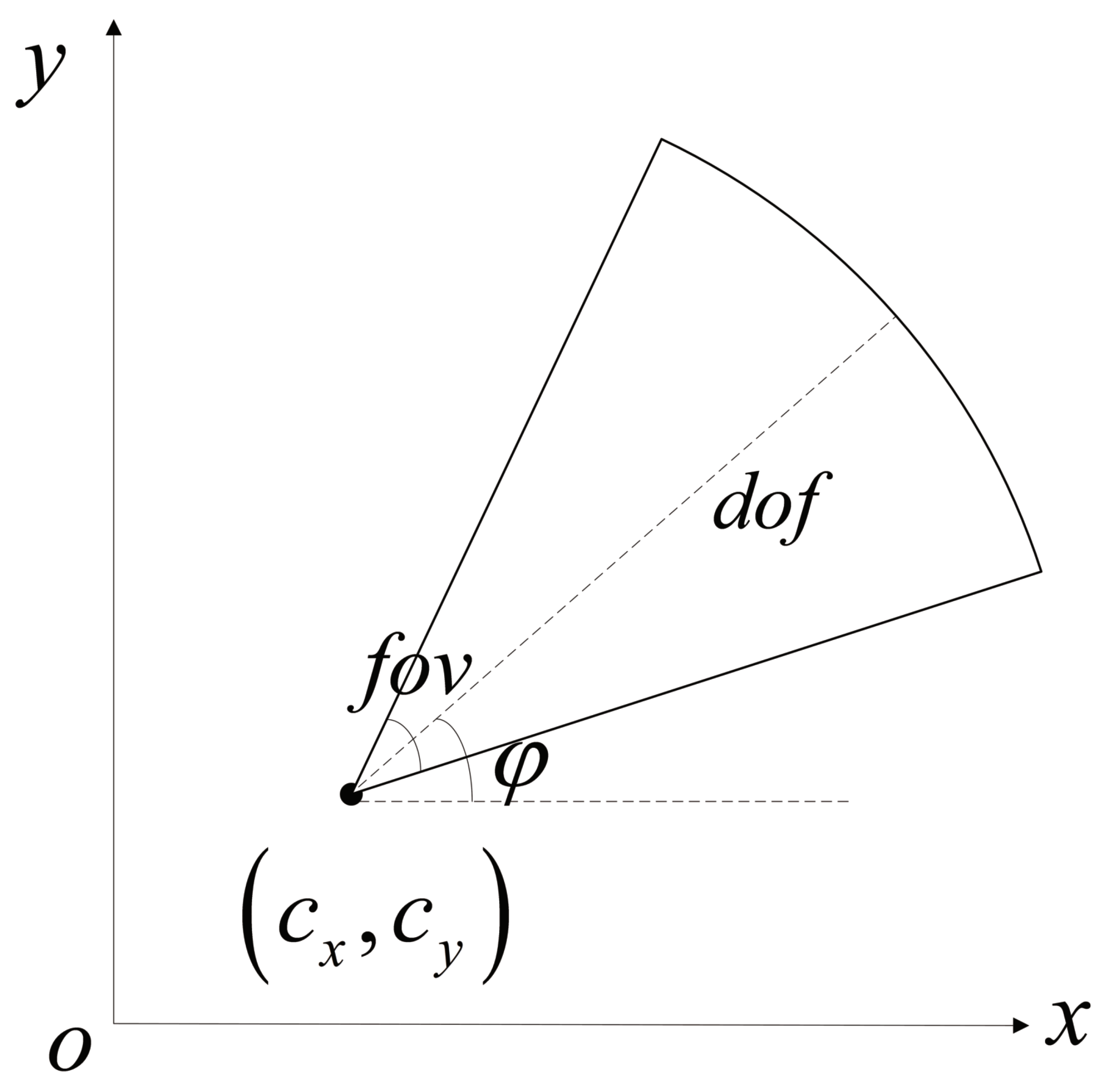
In the 2D problem, the available sensing area of a specific camera could be identified as a circular, triangular, sector, or trapezoid. In this study, as seen in Figure 1, the sensor model is reduced to a sector. The area enclosed by the sector is the camera’s field of view. Consequently, any target object inside the sector is regarded as covered by the camera.

Figure 1.
Camera sensor model.
The camera is located at the vertex of the sector with coordinates . (depth of field) and (field of view), respectively, denote the distance and angle range that a camera is capable of capturing. Azimuth angle of the camera is described by the angle between the angular bisector of angle in the sector area and the positive half of the x axis. Thus, ternary parameter can be used to represent the state of a given type of camera, and .
Based on the mathematical derivation, the following three linear inequality constraints can be used to express the coverage area of a specific camera sensor:
2.3. Space Model
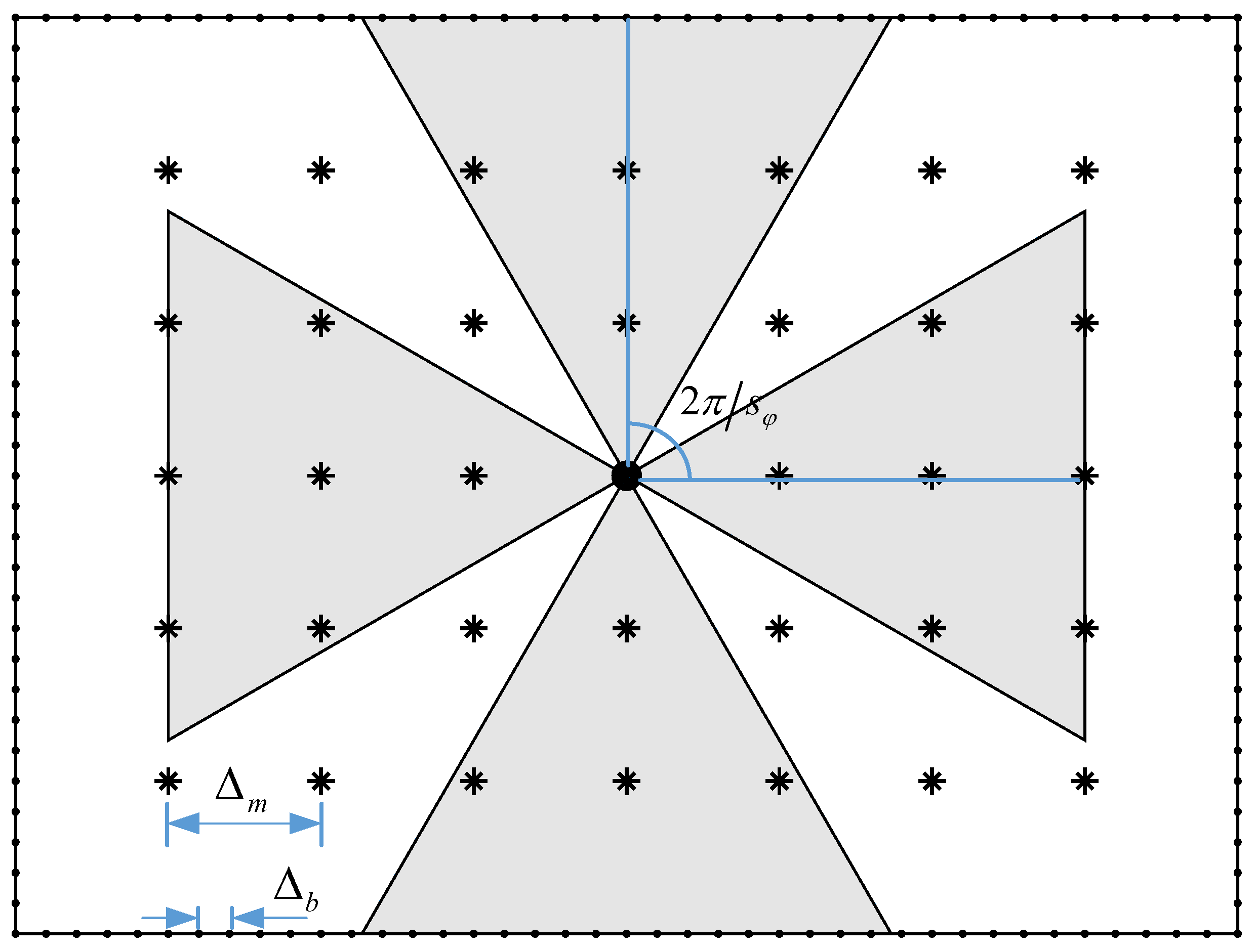
As shown in Figure 2, the space model of this problem can be abstracted as a rectangle. Boundary and measuring area comprise the two components of target space , and they satisfy conditions . A point in the target space is called a working point, denoted by . Since this paper focuses on the coverage and reconstruction problems inside the measurement area, we have . In fact, when we optimize coverage for a given target area, the sensor can only be placed on the boundary, i.e., .
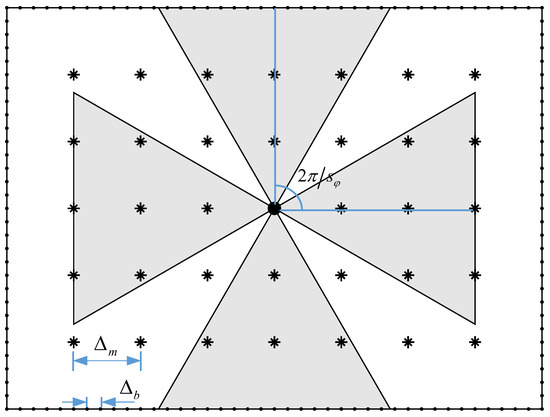
Figure 2.
Uniform sampling of a 2D rectangle target space.
Ideally, the layout of the sensors is a continuous problem, i.e., are continuous variables and can take any value in constraint set . The results obtained by solving continuous optimization problems are generally accurate global solutions, but the algorithm complexity is high. Therefore, considering that the number of sensors is an integer and the sensors’ positions can be sampled, we describe the problem as a discrete optimization problem. Although the optimal solution cannot be guaranteed in this way, a reasonable solution can be found within reasonable time. By sampling the target space into a grid of points, continuous problems can be transformed into discrete problems.
Using the uniform grid sampling model, boundary , measurement area and azimuth angle are uniformly sampled, and the sampling intervals are , and respectively. And is the number of sampling points in azimuth angle . It is considered that in order to guarantee the accuracy of the layout plan. Boundary has and sample points on the x and y axes, respectively, whereas measurement area has and sampling points on the x and y axes, respectively, once the sampling interval is determined. It is shown in Figure 2 that . Therefore, the value ranges of could be a finite set of discrete points, and the continuous problem is transformed into a discrete problem.
2.4. Coverage Model
The study uses the coverage model, which indicates that a space point is either covered and represented as 1 or not covered and represented as 0. In this paper, space points that satisfy Formula (2) are covered, and otherwise are not covered. The degree of coverage for the target space can also be expressed as follows: the degree of coverage for any point in the target space region is k if at least k sensor nodes are covering it at the same time. Considering the need to implement the object tracking and localization task as well as the image reconstruction principle, it is required that the moving object be captured by at least two cameras at the same time, i.e., the sensor network degree of coverage is required. Subsequent modeling and experimental procedures provide scenario-specific k according to the specific scenario.
2.5. Reconstruction Error Model
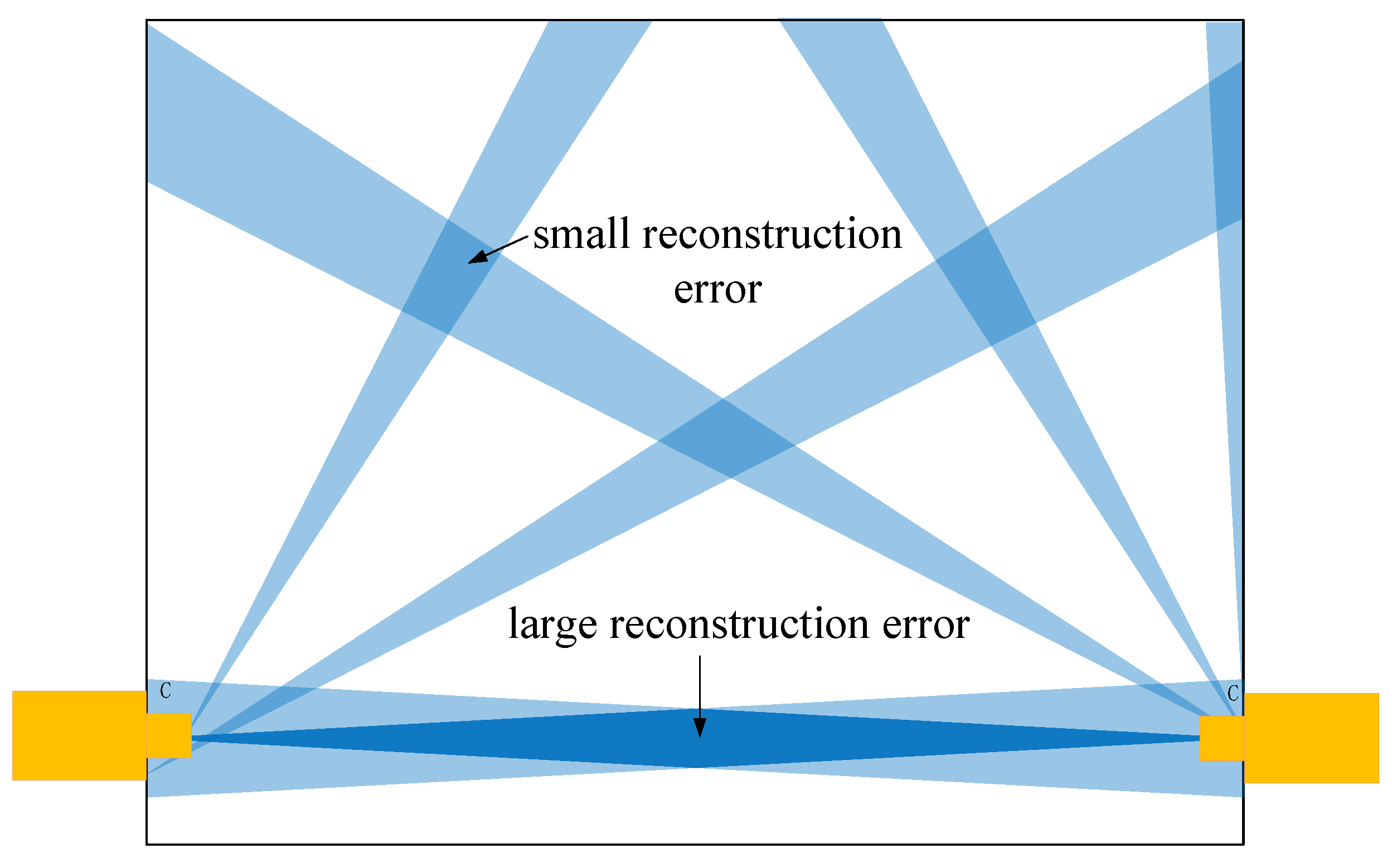
As shown in Figure 3, a simple rectangular environment with two cameras placed opposite each other at the boundary edges is given to clarify the influence of sensor spatial position uncertainty on reconstruction results. The vision sensor can be considered as an orientation sensor to measure the azimuthal angle to the target point, and the uncertainty range of angle measurement is indicated by a light blue triangle. Based on the measurements of the two sensors, the reconstructed coordinates of the target point can be obtained by solving the triangulation method. The two triangular overlapping regions indicate the reconstruction region of this target point, and the size of the region characterises the size of the uncertainty in the position reconstruction, i.e., the reconstruction error. In this case, the dark blue region on the line connecting the two sensors indicates low reconstruction accuracy, while the smaller blue regions in the upper and lower halves indicate high reconstruction accuracy [20]. It can be seen that the positional uncertainty on the straight line between the two sensors is high due to the geometric properties of the sensors. Therefore, if the target point is located in this region, the reconstruction error is higher.
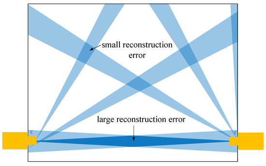
Figure 3.
The reconstruction uncertainty of two camera sensors, where C stands for camera.
The relationship between the reconstruction error and the camera placement strategy is explained in the preceding qualitative analysis. In order to obtain the reconstruction error model resulting from the geometric features of the sensor placement in greater detail, in [29], Kelly defined a geometrical precision factor (GDOP, Geometric Dilution of Precision) to map sensor measurement error to triangulation reconstruction error, which is a measure of positioning uncertainty of each point in the working space caused by the two sensors observing it.
The pose of the target object can be defined by the following vector:
The visual measurements are represented by vector , which is connected to the state vector using a general nonlinear function:
In some particular cases, the relationship may be linear or invertible (state x is determined as an explicit function of measurement z), and the above measurement Model (4) is applicable more generally. It is noted that each element of the measurements poses a constraint on the estimated state. Therefore, the system state can be solved when sufficient constraints are available. However, it is expected that the measurements may be corrupted by additive errors such as noises and disturbances. We suppose that the visual measurements are disturbed by error :
where error may be a systematic measurement error or a random error. We let be the Jacobian matrix of the measurement model. The relationship between measurement error and system state error is as follows:
In general, attention needs to be paid to how the sensor measurement error is amplified into the pose parameter error to be estimated. In this way, a geometric precision factor can be loosely defined as
where and , respectively, represent the measurement of sensor pose error and observation error under any quantitative standard. The mapping between the sensor error and the pose error is in the form of a matrix, and any norm of the matrix can measure the relative magnification of the mapping. The Jacobian determinant is a convenient choice among the available norms because it avoids the calculation of eigenvalues. The Jacobian determinant, then, denotes a scalar multiplier when the Jacobian matrix is square, and it converts the differential volume in the pose space to the corresponding differential volume in the measurement space, which is described as
where , represent the absolute value of the product of the components in pose error vector and observation error vector , respectively, and are a measure of the error range. is the absolute value of the Jacobi determinant; then,
It is noted that the relationship between determinants and the volume of parallel polyhedra is used here, and the following theorem is available in the literature [30], p. 232.
Assuming that , matrix transformation T: meets . If S denotes any region in , then we have
where denotes the mapping of region S after matrix transformation T, and denotes the region volume.
In a more general case, the measurements are implicit functions as
Similarly, when the system is fully determined, we have the definition as
where and are Jacobian matrices, which are both square.
2.6. Reduced Dimensional Search
Based on the analysis above, the sensor position information in a 2D target space can be denoted by , where represents the sensor position and represents the azimuth angle. This positional information determines sensor coverage and the reconstruction error of the target point covered by this sensor. Therefore, in the study of the sensor layout problem, the rational planning of this parameter combination is the key to solve it.
However, most environments have restrictions on the location of sensors, such as in our article, where sensors can only be deployed on four sides of a rectangle. Therefore, in this paper, we design a method to search for sensor location information using one-dimensional parameters to represent sensor location information in the solution space dimensionality reduction search method.
We set the origin of the rectangular coordinate system as the starting point, and move counterclockwise along the boundary of the target space; then, each discrete point on the boundary uniquely corresponds to moving forward distance d. With the previous direction distance representing the position information of the sensor, 2D position parameters can be reduced to 1D distance parameters. This method can reduce optimization parameters and improve running speed. In addition, since the sensor position is defined by only one parameter of the forward distance, for an irregularly shaped space, as long as the mathematical expression of the space boundary is known, the dimensionality reduction technique can take effect as well.
3. Optimization Algorithms
This section uses the basic models introduced above to establish the coverage rate and reconstruction error functions for a 2D space. Then, based on the characteristics of the two objective functions, a method for establishing a multi-objective optimization function is proposed, followed by a suitable multi-objective optimization algorithm to solve the sensor placement optimization problem.
3.1. Coverage
One goal of this optimization problem is to maximize the coverage of the sensor network. After the target space is discretized sampled, binary variable is defined using the discretized sensor pose parameters and measuring point coordinates:
where . and represent the number of sampling points along the x-axis and the y-axis, respectively. After converting the above discrete values into coordinates and angles in the continuous target space, the value of can still be calculated by Inequalities (2). During the simulation process, all values are calculated in advance and stored in a matrix.
After determining the parameter combination and sensor layout scheme, we define matrix , where the elements are
where can be calculated using Formula (13). After that, the quantity of sensors covering the jth point can be expressed as
Additionally, we let a binary variable represent whether or not grid point j complies with the k-coverage criterion, which is described as
Consequently, the total number of sampling points in the measurement region that are covered by at least k sensors is
Lastly, the ratio of the number of sampling points covered to the total number of sampling points defines the coverage r of the target space,
This results in the establishment of a quantitative criterion for evaluating the target space’s coverage. Maximizing r (i.e., maximizing when and already determined) in Equation (18) is necessary to guarantee that the target space is covered to the greatest extent possible.
3.2. Reconstruction Error
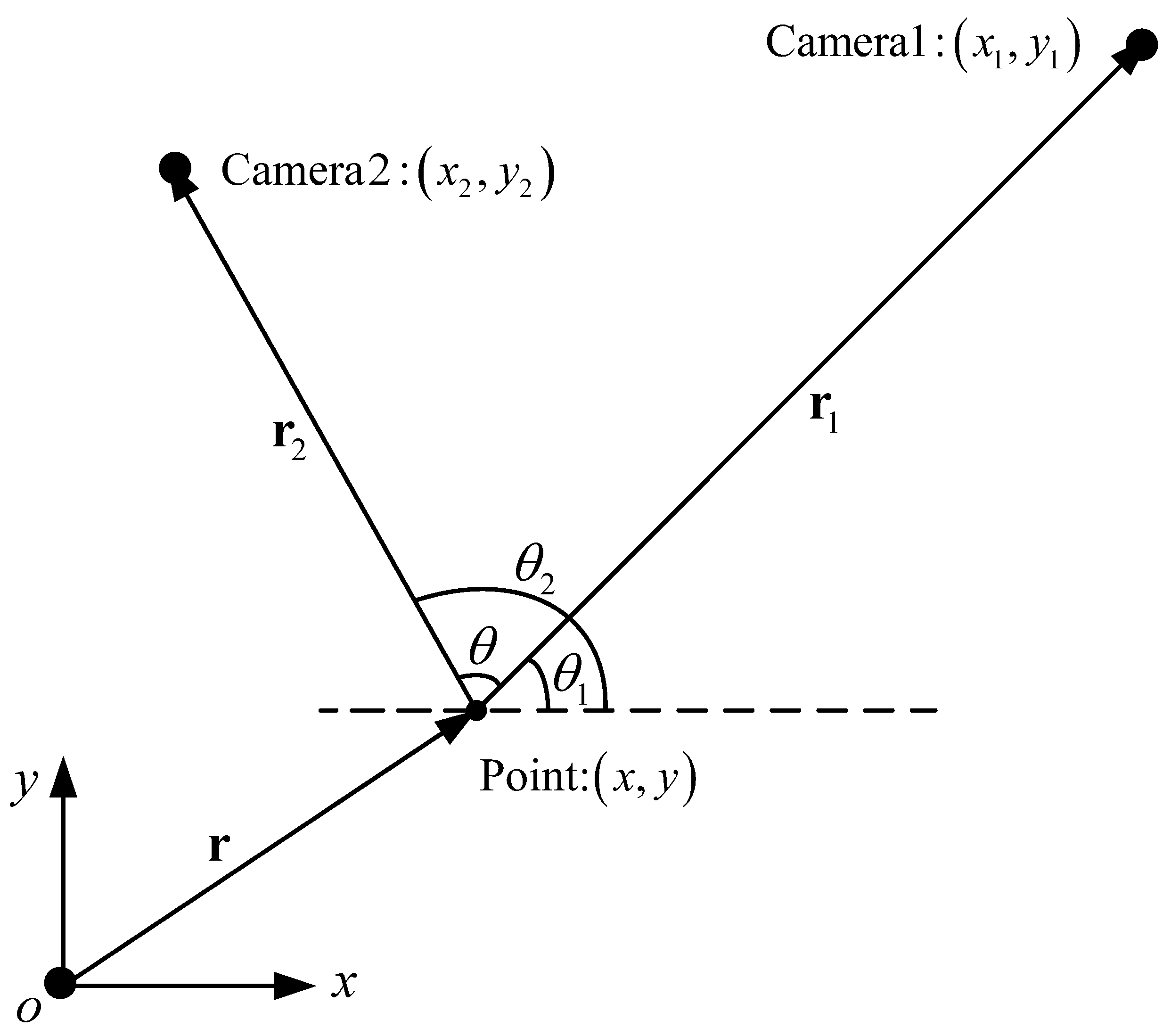
A two-camera system triangulation scheme is described in Figure 4 to explain the reconstruction principle of VSNs in a 2D space. As a kind of directional sensor, the camera can measure the target point’s azimuth angle with respect to itself. Thus, the target point must be the intersection of two rays with known azimuth angles starting from the two cameras. With the two angle constraints, the target point is reconstructed by a triangulation method.

Figure 4.
Schematic diagram of the principle of 2D spatial reconstruction.
As shown in Figure 4, the coordinates of the two visual sensors are and , and the azimuth angles of the target point relative to themselves are and . Here, angles and are defined as the counterclockwise angle from the positive semi-axis of the x axis, and the ranges are in . We define and as the distance vectors of the two vision sensors relative to the target point, and their modulus lengths are and . According to the derivation process in reference [29], the intersection meets the following constraints:
The measurement model is an implicit function as Equation (11) with definition and . Then, the Jacobian matrix is square, and the Jacobian determinant is calculated as
where . Then, the determinant has the form of
where is defined as convergence angle and .
Therefore, the GDOP is calculated as
Based on the above derivation, GDOP is equal to the product of the distance from the two vision sensors to the target point and the cosecant value of convergence angle . When the target point is on the line connecting the two sensors (), the GDOP tends to infinity; when the convergence angle between the two sensors becomes larger, the GDOP decreases. GDOP reaches its minimum when the convergence angle of the two sensors is a right angle, and the target is close to the sensor.
Based on Equation (22), GDOP measures the degree to which the sensor measurement error is amplified into the reconstruction error during the reconstruction process. Therefore, the quality of the reconstruction result can be represented by the reciprocal of GDOP. To confine the quality function to , a suitable scale factor, , is chosen, and sensors i and to target location j’s reconstruction quality function can be obtained as follows:
The expression of is shown in Equation (14), and these values guarantee the reconstruction quality to be zero when sample point j is not 2-coverage. It is worth mentioning that the above quality function can be extended based on the basic model employed. For example, if a probability coverage model rather than a binary coverage model is used, the coverage probability can multiply. In addition, more than two cameras may cover the target point at the same time. Reconstruction quality of target point j is set to the highest of all potential camera pairs that can cover in order to increase the average reconstruction quality. Thus, we can obtain
where reconstruction quality of each pair of sensors to the target point is defined in Formula (23). After traversing each sampling point in the target space, the average reconstruction quality of the whole area can be found as follows:
We note that average reconstruction quality q is inversely proportional to the average reconstruction error. The higher the average reconstruction quality, the smaller the average reconstruction error. So both variables reflect the measurement accuracy of the system. In order to unify the optimization method with the coverage function, this paper takes the maximization of average reconstruction quality q as an optimization objective.
3.3. Multi-Object Optimization
Based on the mathematical models established in the previous parts, as well as 2D space coverage r and average reconstruction quality q, the primary purpose of this subsection is to establish a multi-objective optimization function that takes the characteristics of these two objective functions into account. At the same time, an appropriate multi-objective optimization method is constructed to handle the sensor placement optimization problem.
In practical applications, it is often necessary to consider both coverage and reconstruction error. The coverage and reconstruction quality can be calculated by Formulas (18) and (25), respectively. As can be observed, the two evaluation index values, coverage r and reconstruction quality q, have the same order of magnitude and fall inside the range of . Thus, a multi-objective optimization function is established to comprehensively evaluate the performance of the system by calculating their weighted sum:
where the degree to which the coverage is subject to the evaluation criteria is indicated by weighting coefficient . When , the evaluation criterion is to maximize the coverage; when , it is to maximize the reconstruction quality, i.e., to minimize the reconstruction error.
To sum up, the sensor placement optimization problem in this paper can be abstracted as the following nonlinear optimization problem:
where , N is the number of cameras.
The above process converts sensor pose parameters into discrete variables through an equidistant sampling of space and angle. Meanwhile, the target space is uniformly sampled into a set of grid points. By applying geometric relations to calculate the coverage and reconstruction error of each sampling point, we thus establish a discrete model of the sensor layout problem. This method can simplify the model, speed up the calculation, and then maintain the accuracy required for the task.
In order to tackle the discrete optimization problem (27), this research suggests combining the GA and PSO algorithms. GA has been proven to be an effective method for optimizing sensor configuration and for determining the position of attitude sensors. The optimization process of GA does not rely on gradients or other additional information, and the search results can be used as the near-optimal solution to the problem. Still, these results depend on the initial value (initial population). When the initial value is not correctly selected, the algorithm’s performance may be affected. On the other hand, PSO is one of the best-known nature-inspired algorithms, inspired by information loops and social behaviors such as bird flocking and fish flocking. This is a global optimization algorithm, especially suitable for solving problems where the optimal solution is a multi-dimensional space parameter. Each particle in the group represents a solution in the solution space. The algorithm solves the problem intelligently through the movement of individual particles and the exchange of information within the group. Due to its simplicity in implementation and fast convergence speed, PSO is widely used. But it still suffers from problems such as dimensionality explosion, and it can easily fall into a local optimum since it convergences too fast.
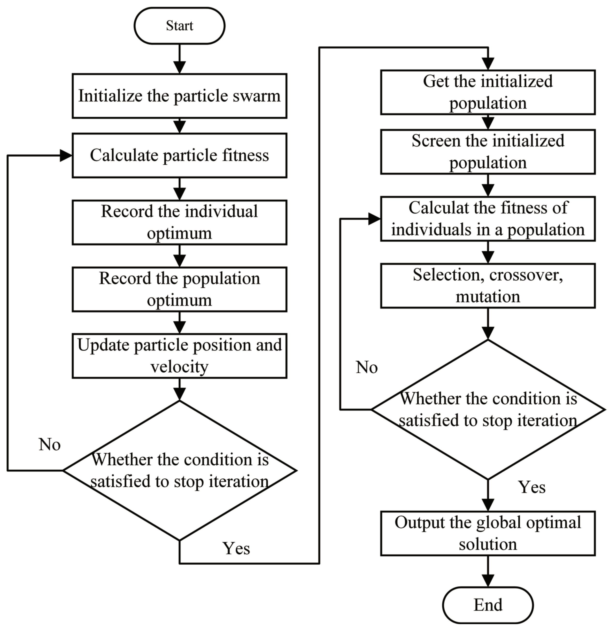
Through the above analysis, it is shown that both GA and PSO have advantages and disadvantages. Therefore, in this section, a combined algorithm is proposed to merge the advantages of the PSO and the GA. First, the PSO is used, and the result is taken as the initial value of the GA, which can reduce the running time, improve the efficiency of the algorithm, and avoid the algorithm falling into the local optimal solution as far as possible. Figure 5 is a flowchart illustrating the combined algorithm.
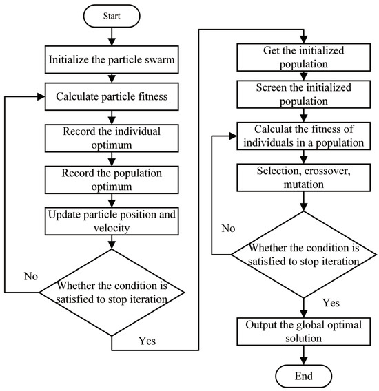
Figure 5.
Flowchart of the combined algorithm.
4. Experimental Evaluation
In this section, extensive simulation experiments are carried out to evaluate the proposed camera placement optimization algorithm. All the simulation experiments are executed on a laptop with the following specifications: Intel Core i7-1065G7 CPU @1.3GHz , 16 GB RAM, in which the environmental parameters, sensor parameters and objective functions are reasonably selected according to specific requirements.
4.1. Comparison between Different Objectives
Considering that in the application of VSNs, there may be different actual requirements for different application scenarios corresponding to different optimization objectives, this section assumes some possible real scenarios and conducts simulation experiments to verify the correctness of the perceptual coverage model and the optimization algorithm. There are three different scenario models, i.e., maximum 1-coverage, maximum 2-coverage, and maximum both 2-coverage and reconstruction quality. We assume that the target space is a 2D plane of without any obstacle and that the camera type and parameters are the same. In this experiment, the sampling and camera parameters are set as = 5 m, = 5 m, = 4, = 37°, = 65 m.
The first objective is a simple situation where only a simple monitoring is needed, that is, each point in the target area only needs to be covered by at least one sensor, and no constraints on the reconstruction accuracy are required. Figure 6a shows the effect of using four cameras to achieve the maximum 1-coverage objective, and it can be observed that full coverage is achieved with nearly no overlapping area, avoiding the waste of resources.
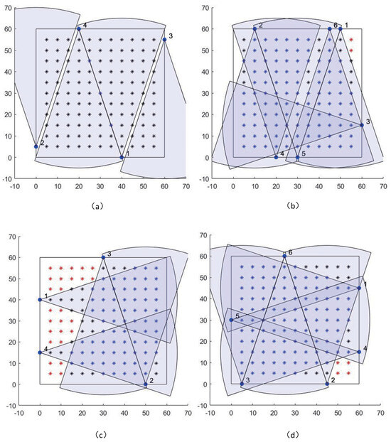
Figure 6.
Comparisons of optimal camera placements under different objectives. (a) Maximized 1-coverage with four cameras; (b) maximized 2-coverage with six cameras; (c) maximized 2-coverage and reconstruction quality with four cameras; (d) maximize the 2-coverage and reconstruction quality with six cameras. We note that the red, black and blue star symbols represent the space points which are simultaneously covered by no, one and two camera sensors, respectively. Solid blue dots represent cameras, and the blue sector represents the coverage area of the cameras.
The second objective considers the situation where a larger portion of the target space needs to be covered by at least two sensors while no constraints on the reconstruction accuracy are imposed. The effect of four cameras to achieve 2-coverage was tested, and it was found that the coverage to satisfy 2-coverage could only rise up to 50% at most. Therefore, it was necessary to increase the number of cameras to achieve the 2-coverage objective. Figure 6b shows the effect of using six cameras to achieve the maximum 2-coverage objective. It can be seen that the coverage of the whole target area is good (81% network coverage) and mainly in the middle activity area; however, some sensors are close to each other (e.g., 1 and 6), which may lead to larger reconstruction error in the overlapping areas of their coverage. Since no evaluation metrics for reconstruction error were included, this result is as expected.
Since the position of a space point can be reconstructed only when at least two camera sensors observe it using the triangulation method, we select the maximum 2-coverage as the third objective because we want to discuss reconstruction quality. Figure 6c,d show the effects of using four and six cameras to achieve the third objective, i.e., maximizing the 2-coverage and reconstruction quality, respectively. As can be seen, the sensor layouts are reasonable, and there are no instances of two cameras in close proximity. Furthermore, it is clear that the coverage with six cameras is superior to the coverage with four cameras. The results of the experiment show that the coverage with four cameras is 48%, while with six cameras it is 75%.
4.2. Comparison between Different Approaches
This subsection discusses the results of comparative experiments with different optimization algorithms, including the PSO, the GA, and their combined algorithms. Based on experience and repeated experiments, the parameters of the GA are set as follows: the crossover probability is , the mutation probability is , the population size is 50, and the number of iterations depends on the size of the optimization problem. The parameters of the PSO are set as follows: , the number of populations is 50, and the number of iterations depends on the size of the optimization problem. Three sets of parameter combinations were designed to validate these algorithms for the 2D space, and finally, their performances were compared. Three sets of different parameter combinations are shown in Table 1.

Table 1.
Different parameter combinations for comparison of the different approaches.
For each parameter combination, the average running time, average coverage, and standard deviation of the coverage are recorded in Table 2. It can be seen that the combined algorithm consistently produces the best optimization results, and the standard deviations are all smaller than the other two algorithms, which indicates that the combined algorithm produces better and more stable optimization results. In addition, the average running time of the combined algorithm is between that of the PSO and the GA, with a significant reduction in running time compared to the GA. Among the three algorithms, PSO has always had the lowest running time, as well as the lowest coverage, and the optimization results are unstable, probably because PSO can easily fall into a local optimum and cannot obtain the global optimal solution.

Table 2.
Experimental results for comparison of the different approaches.
4.3. Comparison between Different Sampling Parameters
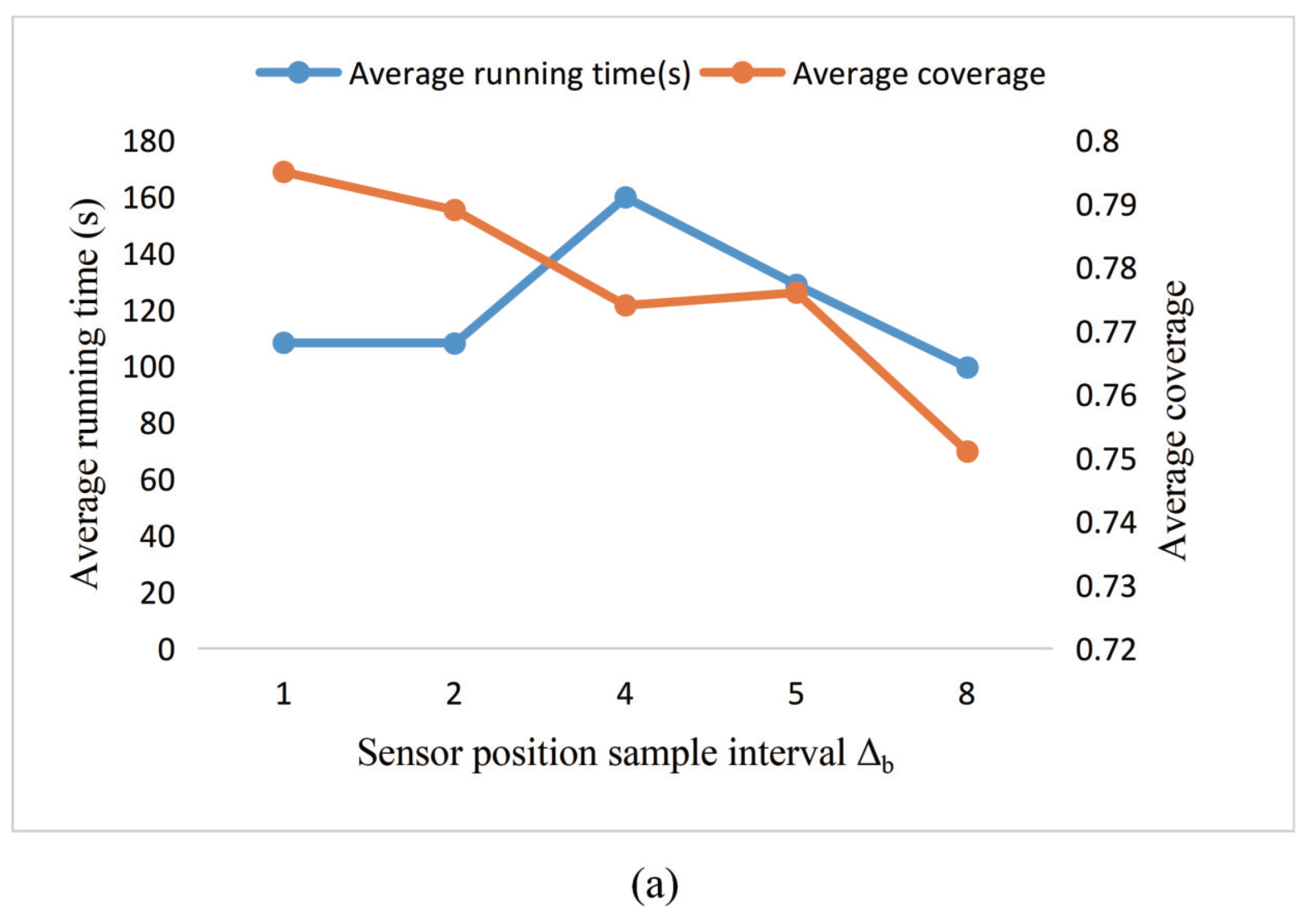
In order to analyze the influence of sensor sampling parameters on optimization results, this subsection uses different sampling parameters to compare the average running speed and the average coverage rate of the space. Concretely, we discuss the influence of sampling parameters on optimization results.
Qualitatively speaking, sensor position sampling interval determines the discrete values of sensor coordinates that can take in the optimization. The smaller the , the more discrete the coordinate values that can be taken, and, accordingly, the larger the solution space to be searched. Similarly, the sampling number of sensor azimuth angle determines the discrete value that the sensor azimuth angle can take in the layout. The larger the , the more discrete values the azimuth can take, and accordingly the larger the solution space the algorithm needs to search. To simplify the optimization process, we choose the GA to be the algorithm and 1-coverage as the objective. But the conclusions could also be applied to more complicated situations.
As shown in Figure 7a, as the sampling interval of the sensor position increases, there is a general downward trend in average coverage due to degradation in model accuracy. It is worth noting that the change in running time is not so noticeable. The possible reason is that the sampling interval increases, the solution space that needs to be searched becomes smaller, and then the search process seems to become faster. However, when there is more than one optimal placement scheme, but with fewer search options available, some solutions are missed, which reduces the number of optimal options available. Therefore, the difficulty in searching increases, and the search time is not significantly reduced. Figure 7b shows the results of different sampling numbers of the sensor azimuth angle. It is found that, as the number of sensor azimuth sampling points increases, the average running time increases, but the coverage does not increase steadily. The possible reason for this situation is that the experiment uses a relatively simple rectangular unobstructed target space. The four optional azimuths can already satisfy the necessary coverage requirements, so a slight increase in sampling points cannot significantly improve optimization performance.

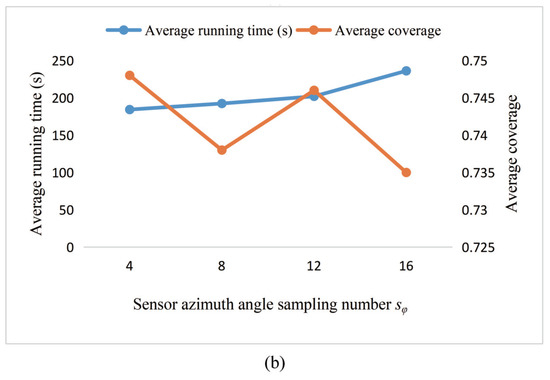
Figure 7.
Experimental results for a comparison of the different sampling parameters. (a): The influence of sensor position sample interval on the results; (b) the influence of the sampling number of sensor azimuth angle on the results.
4.4. An Obstruction Situation
The studies mentioned above take into account the scenario in which the target space contains no obstacles; however, this is rarely the case in real life. In this research, we present a sensor coverage approach using one corridor of Daxing Airport Terminal as an example, which is a big target space containing obstacles.
Daxing Airport Terminal is the second largest airport terminal in the world, with a total floor area of 1.03 million square meters. And its architecture is unique, offering travelers wide and comfortable waiting spaces as well as business and service facilities. However, the area is densely populated and the passenger flow is large, which brings huge pressure to security work. Therefore, it is of great significance to optimize camera coverage in this area.
Figure 8 shows the optimization effect of camera coverage in the corridor. In this experiment, the sampling interval is 15 m, and the green area represents the coverage of the camera, where the of the camera is 60 m and the is 37°. By adjusting the layout of the camera, full coverage of the target space with obstacles can be achieved. We can adjust the sampling interval and the and of the camera according to the actual needs. We will conduct a more thorough investigation on this topic in the future; this is merely an overview of the situation with obstacles.
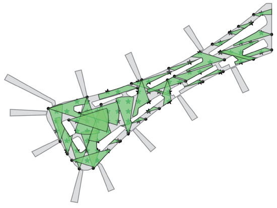
Figure 8.
The optimization effect of camera coverage in one corridor of Daxing Airport Terminal. The various white irregular boxes in the figure represent the business and office area and other public facilities. The five-pointed stars in the figure represent sampling points. Solid black dots represent cameras, and the green sector represents the coverage area of the cameras.
5. Conclusions
In this paper, we propose a sensor placement optimization method that conserves network resources and improves facilities management. This proposed method first builds some models as a basis for the optimization process and proposes a reduced dimensional search method. Then, a multi-objective optimization function is designed to balance the coverage and reconstruction error, and a combined optimization algorithm is used. Lastly, comparative experiments are used to show the method’s effectiveness and reasonableness, and a coverage optimization method for a wide target space with obstacles is presented. However, the method proposed in this paper can be improved in a few ways. The current research on this problem is still focused on the 2D level, but further research can extend the proposed models and algorithms to the 3D domain. And scenarios with obstacles require further study. But our method has very broad development prospects and can be used in subway stations, airport terminals, and other densely populated areas of the camera layout.
Author Contributions
Conceptualization, H.D. and Z.Z.; methodology, J.Z., H.D. and Z.Z.; software, J.Z., H.D. and X.W.; validation, J.Z. and Y.Z.; formal analysis, J.Z.; investigation, J.Z. and H.D.; resources, H.D. and Z.Z.; data curation, J.Z. and H.D.; writing—original draft preparation, J.Z., Y.Z. and X.W.; writing—review and editing, J.Z. and Y.Z.; visualization, J.Z. and H.D.; supervision, H.D.; project administration, H.D. and Z.Z.; funding acquisition, H.D. and Z.Z. All authors have read and agreed to the published version of the manuscript.
Funding
This work is supported by the National Natural Science Foundation of China (NSFC, Grant No. 62203023).
Institutional Review Board Statement
Not applicable.
Informed Consent Statement
Not applicable.
Data Availability Statement
The raw data supporting the conclusions of this article will be made available by the authors on request.
Conflicts of Interest
The authors declare no conflict of interest.
References
- Hu, Q.; Zhang, Y.; Xie, X.; Su, W.; Li, Y.; Shan, L.; Yu, X. Optimal placement of vibration sensors for industrial robots based on bayesian theory. Appl. Sci. 2022, 12, 6086. [Google Scholar] [CrossRef]
- Estrada, E.; Martinez Vargas, M.P.; Gómez, J.; Peña Pérez Negron, A.; López, G.L.; Maciel, R. Smart cities big data algorithms for sensors location. Appl. Sci. 2019, 9, 4196. [Google Scholar] [CrossRef]
- Giordano, J.; Lazzaretto, M.; Michieletto, G.; Cenedese, A. Visual Sensor Networks for Indoor Real-Time Surveillance and Tracking of Multiple Targets. Sensors 2022, 22, 2661. [Google Scholar] [CrossRef] [PubMed]
- Jun, S.; Chang, T.W.; Yoon, H.J. Placing visual sensors using heuristic algorithms for bridge surveillance. Appl. Sci. 2018, 8, 70. [Google Scholar] [CrossRef]
- AbdelTawab, A.M.; Abdelhalim, M.; Habib, S. Moving Object Detection over Wireless Visual Sensor Networks using Spectral Dual Mode Background Subtraction. Int. J. Adv. Comput. Sci. Appl. 2022, 13. [Google Scholar] [CrossRef]
- Idoudi, M.; Bourennane, E.B.; Grayaa, K. Wireless visual sensor network platform for indoor localization and tracking of a patient for rehabilitation task. IEEE Sens. J. 2018, 18, 5915–5928. [Google Scholar] [CrossRef]
- Arnold, E.; Dianati, M.; de Temple, R.; Fallah, S. Cooperative perception for 3D object detection in driving scenarios using infrastructure sensors. IEEE Trans. Intell. Transp. Syst. 2020, 23, 1852–1864. [Google Scholar] [CrossRef]
- Du, R.; Santi, P.; Xiao, M.; Vasilakos, A.V.; Fischione, C. The sensable city: A survey on the deployment and management for smart city monitoring. IEEE Commun. Surv. Tutorials 2018, 21, 1533–1560. [Google Scholar] [CrossRef]
- Xie, H.; Low, K.H.; He, Z. Adaptive visual servoing of unmanned aerial vehicles in GPS-denied environments. IEEE/ASME Trans. Mechatronics 2017, 22, 2554–2563. [Google Scholar] [CrossRef]
- Savkin, A.V.; Huang, H. A method for optimized deployment of a network of surveillance aerial drones. IEEE Syst. J. 2019, 13, 4474–4477. [Google Scholar] [CrossRef]
- O’rourke, J. Art Gallery Theorems and Algorithms; Oxford University Press: Oxford, UK, 1987; Volume 57. [Google Scholar]
- Sourav, A.A.; Peschel, J.M. Visual Sensor Placement Optimization with 3D Animation for Cattle Health Monitoring in a Confined Operation. Animals 2022, 12, 1181. [Google Scholar] [CrossRef]
- Tveit, V. Development of Genetic and GPU-Based Brute Force Algorithms for Optimal Sensor Placement. Master’s Thesis, University of Agder, Kristiansand, Norway, 2018. [Google Scholar]
- Altahir, A.A.; Asirvadam, V.S.; Hamid, N.H.B.; Sebastian, P.; Hassan, M.A.; Saad, N.B.; Ibrahim, R.; Dass, S.C. Visual sensor placement based on risk maps. IEEE Trans. Instrum. Meas. 2019, 69, 3109–3117. [Google Scholar] [CrossRef]
- Kelp, M.M.; Lin, S.; Kutz, J.N.; Mickley, L.J. A new approach for determining optimal placement of PM2.5 air quality sensors: Case study for the contiguous United States. Environ. Res. Lett. 2022, 17, 034034. [Google Scholar] [CrossRef]
- Chebi, H. Proposed and application of the Dragonfly algorithm for the camera placement problem. In Proceedings of the 2022 IEEE 9th International Conference on Sciences of Electronics, Technologies of Information and Telecommunications (SETIT), Hammamet, Tunisia, 28–30 May 2022; pp. 503–509. [Google Scholar]
- Puligandla, V.A.; Lončarić, S. A multiresolution approach for large real-world camera placement optimization problems. IEEE Access 2022, 10, 61601–61616. [Google Scholar] [CrossRef]
- Ali, A.; Hassanein, H.S. Optimal Placement of Camera Wireless Sensors in Greenhouses. In Proceedings of the ICC 2021-IEEE International Conference on Communications, Montreal, QC, Canada, 14–23 June 2021; pp. 1–6. [Google Scholar]
- Zhang, G.; Dong, B.; Zheng, J. Visual sensor placement and orientation optimization for surveillance systems. In Proceedings of the 2015 10th International Conference on Broadband and Wireless Computing, Communication and Applications (BWCCA), Krakow, Poland, 4–6 November 2015; pp. 1–5. [Google Scholar]
- Kirchhof, N. Optimal placement of multiple sensors for localization applications. In Proceedings of the International Conference on Indoor Positioning and Indoor Navigation, Montbeliard, France, 28–31 October 2013; pp. 1–10. [Google Scholar]
- Altınel, İ.K.; Aras, N.; Güney, E.; Ersoy, C. Binary integer programming formulation and heuristics for differentiated coverage in heterogeneous sensor networks. Comput. Netw. 2008, 52, 2419–2431. [Google Scholar] [CrossRef]
- Gonzalez-Barbosa, J.J.; García-Ramírez, T.; Salas, J.; Hurtado-Ramos, J.B. Optimal camera placement for total coverage. In Proceedings of the 2009 IEEE International Conference on Robotics and Automation, Kobe, Japan, 12–17 May 2009; pp. 844–848. [Google Scholar]
- Mozaffari, M.; Safarinejadian, B.; Shasadeghi, M. A novel mobile agent-based distributed evidential expectation maximization algorithm for uncertain sensor networks. Trans. Inst. Meas. Control 2021, 43, 1609–1619. [Google Scholar] [CrossRef]
- Rahimian, P.; Kearney, J.K. Optimal camera placement for motion capture systems. IEEE Trans. Vis. Comput. Graph. 2016, 23, 1209–1221. [Google Scholar] [CrossRef]
- Aissaoui, A.; Ouafi, A.; Pudlo, P.; Gillet, C.; Baarir, Z.E.; Taleb-Ahmed, A. Designing a camera placement assistance system for human motion capture based on a guided genetic algorithm. Virtual Real. 2018, 22, 13–23. [Google Scholar] [CrossRef]
- Zhang, X.; Zhang, B.; Chen, X.; Fang, Y. Coverage optimization of visual sensor networks for observing 3-D objects: Survey and comparison. Int. J. Intell. Robot. Appl. 2019, 3, 342–361. [Google Scholar] [CrossRef]
- Li, Q.; Yang, M.; Lu, Z.; Zhang, Y.; Ba, W. A soft-sensing method for product quality monitoring based on particle swarm optimization deep belief networks. Trans. Inst. Meas. Control 2022, 44, 2900–2910. [Google Scholar] [CrossRef]
- Hocine, C.; Benaissa, A. New Binary Particle Swarm Optimization Algorithm for Surveillance and Camera Situation Assessments. J. Electr. Eng. Technol. 2021, 1–11. [Google Scholar] [CrossRef]
- Kelly, A. Precision dilution in triangulation based mobile robot position estimation. Intell. Auton. Syst. 2003, 8, 1046–1053. [Google Scholar]
- Margalit, D.; Rabinoff, J.; Rolen, L. Interactive Linear Algebra; Georgia Institute of Technology: Atlanta, GA, USA, 2017. [Google Scholar]
Disclaimer/Publisher’s Note: The statements, opinions and data contained in all publications are solely those of the individual author(s) and contributor(s) and not of MDPI and/or the editor(s). MDPI and/or the editor(s) disclaim responsibility for any injury to people or property resulting from any ideas, methods, instructions or products referred to in the content. |
© 2024 by the authors. Licensee MDPI, Basel, Switzerland. This article is an open access article distributed under the terms and conditions of the Creative Commons Attribution (CC BY) license (https://creativecommons.org/licenses/by/4.0/).

