Abstract
To estimate earthquake losses for regional buildings, it is important to consider the varying seismic performances of different types of buildings. To achieve this, a dynamic elastic–plastic analysis based on detailed structural modeling is more accurate than the capacity spectrum method based on a single degree of freedom to obtain the response and damage of various structures under seismic activity and provide a more precise estimate of earthquake losses for buildings. Detailed information about the building facilities is necessary to create a fine structural model. However, obtaining precise actual structural details can be challenging with existing methods, especially when there are a large number of buildings to consider. This paper proposes a new method called story-based random structure (SBRS) modeling to address this issue, which is based on the common and reasonable layout of the structure. The process involves choosing design parameters that can represent the structural arrangement of a building as variables. These parameters include the materials’ type and strength, proportions, the components’ size, and other relevant factors. The values for these variables are determined based on engineering experience and design specifications. The range of values for these variables is also determined to ensure that all design requirements are met. Finally, the Latin Hypercubic Sampling (LHS) method is used to randomly sample and combine the variables, establishing a detailed structural model of the building with structural uncertainty. According to the results of the analysis, this method can simulate the structure and component information of a building by using a probabilistic approach, even without knowing the specific structural design. This method can be based on a small amount of readily available building information and solves the problem of the rapid and refined modeling of a large number of buildings at the regional scale. It also makes it possible to estimate the earthquake loss of regional buildings based on their seismic capacity.
1. Introduction
Currently, earthquake loss estimation methods for regional buildings can be broadly categorized into classification and statistical methods based on historical seismic damage data and elastic–plastic analysis methods based on structural models [1,2]. The former is a data-driven method, and the reliability of the calculation results depends mainly on the accumulation of historical seismic hazard data. In contrast, there is still a need for more historical seismic hazard data [3,4], and their practical application is limited to a certain extent [5]. At the same time, the assessment results of this type of method are biased toward the macro, the assessment accuracy of individual needs to be improved, and it is difficult to reflect the differences between individual buildings of the same type. With the development of the structural finite element method and dynamic nonlinear integration method, the structural model-based elastoplastic analysis method has the advantages of a high accuracy, low cost and equipment needs, and convenient and fast implementation, which has a broader application prospect. The prerequisite for implementing this method is to categorize buildings based on their characteristics and create corresponding simplified models, which is fundamental for conducting large-scale analyses.
HAZUS [6], a widely used regional disaster assessment software from America, can assess and predict the economic losses, casualties, and injuries of buildings and various types of infrastructure caused by earthquakes [7,8], and similar systems have been developed in other countries or regions based on it [9,10,11]. HAZUS categorizes buildings into 36 types based on their construction materials, structural forms, number of stories, and seismic design codes. However, HAZUS is based on the Capacity Spectrum Method (CSM) to simplify all kinds of buildings into a single-degree-of-freedom system. The damaged state of the whole structure is unique, which is not able to reflect the distribution of the loss inside the building, while in practice, the distribution of the loss of the medium- and high-rise buildings tends to be more concentrated in some stories, with a large discrepancy between these stories. Meanwhile, HAZUS uses Push-over analysis to obtain the seismic capacity curve of the building. The seismic response of the structure is only controlled by the first vibration mode while ignoring the influence of higher-order modes, which is a big difference between the results of the response analysis under the condition of ground shaking with impulses in the near-field and the response analysis by taking into account the influence of the higher-order vibration modes [8,11,12]. Moreover, HAZUS needs help with the problem of database adaptability, and the applicability of the seismic hazard model and the repair cost ratios for all levels of damage states are poor for regions outside North America [13], which is significantly different from actual damage.
The Pacific Earthquake Engineering Research Center (PEER) proposed the second generation of Performance-Based Earthquake Engineering (PBEE) [14], which has changed from emphasizing the “mechanical performance” and “safety performance” of structures to highlighting the “economic performance” of structures [15,16]. The seismic performance assessment of buildings methodology [17] published by FEMA best reflects the concept and connotation of the second generation of PBEE. Academics and other stakeholders have widely recognized it since its introduction [18,19]. The methodology divides components with the same seismic demand parameters into performance groups (e.g., shear walls on the same story in the same direction). Based on the fragility function and the consequence function of the performance group, the Monte Carlo method is used to simulate and obtain the building’s economic losses, casualties, and repair time. This methodology can ensure a high computational accuracy, but the premise is that detailed building construction information is required. Due to the enormous workload of information collection, it is mainly used for building-specific seismic performance evaluation or a small number of buildings, and it is challenging to apply it to group buildings at the urban–regional scale.
Ramirez et al. [20] proposed a simplified building earthquake loss estimation method based on the PBEE theoretical framework, which takes the story as the basic unit of response analysis and loss estimation and combines the fragility function of engineering experience with the distribution law of various types of component costs among stories. The framework directly links the seismic demand parameters of the story with the story loss, effectively balancing accuracy and efficiency, which provides a new vision for refined regional earthquake loss estimation. However, this method also requires detailed building construction information, and traditional methods such as field surveys and consulting design data may not be practical for regional buildings. Technical means such as remote sensing mapping cannot obtain the structural arrangement inside the building, which makes it challenging to apply this method to urban group buildings at a regional scale as well.
Lu et al. [5] also established an urban seismic elastoplastic analysis method using the story as the basic unit of structural response analysis for seismic hazard simulation and loss analysis in urban areas. The process is based on a nonlinear multiple-degree-of-freedom (MDOF) model, including a shear model for multistory buildings and a flexural-shear model for high-rise buildings, and the response of the structure under a specific seismic shock is obtained through a dynamic time history analysis, which achieves a better balance between accuracy and computational strength. However, the MDOF model in this method is based on the empirical relationships between the mass of the story and the stiffness and structural self-resonance period, whereas the mass of the story is obtained by multiplying the area of the story (obtained by GIS or based on empirical data) by the empirical mass per unit area [21]. Since these values and empirical relationships are deterministic, when the story area is determined, the modeling developed cannot consider the structural uncertainty due to the unknown parameters of the building contents and layout information and the resulting impact on the seismic capacity and losses of the structure.
The method was also adopted by Zeng et al. [22] for an intensity-based earthquake loss assessment of three typical buildings on the Tsinghua campus, and by combining seismic response with the building component fragility functions and consequences functions in the FEMA-P58 database, the direct earthquake loss and repair time can be obtained. However, the method requires more detailed building construction information, and the information collection workload is extensive, with the establishment of 619 building performance models requiring 11 students for four weeks of work by site survey [23]. Even though it is possible to use the Building Information Model (BIM) for assistance in obtaining detailed information on building components [24], only a relatively small percentage of active buildings have been modeled, and the workload required for large-scale BIM is significant. Therefore, applying this method at a regional scale still needs help in effectively obtaining detailed building construction information and modeling it accurately.
At present, there are five main ways to obtain regional building construction information: based on census data [6], based on geographic information systems (GIS) [25], based on site surveys [26], based on design information [24], and based on empirical data [21]. Building information obtained by census data is usually rough and rarely involves detailed building construction information, such as HAZUS, which divides buildings into 36 categories according to their structural characteristics and use functions and determines the ratio of the number of each type of building in the region based on zoning census data, and determines the difference in losses between different individuals of the same kind of building by floor area, which cannot consider the impact of the differences in the internal construction on the seismic performance and earthquake losses. The GIS-based approach faces the same problem. Ruggieri et al. [26] conducted field surveys to gather architectural information on masonry structures, and the collected information was classified into two categories: deterministic parameters and uncertain parameters. Archetypes, which are ideal representations of existing building stock, were created to model the geometrical and mechanical uncertainties of buildings. Although the process based on field surveys or design data can obtain detailed building construction information, it is more labor-intensive and time-consuming. It can be used for small-scale regional building information surveys in neighborhoods and streets, but it is challenging to apply it to an urban–regional scale. The method based on empirical data is similar to that founded on census data, which gives the proportion of the number of various types of buildings in the region and can only differentiate the differences between buildings by structural kind, but cannot distinguish the individual differences between similar buildings without knowing the specific structural design.
Therefore, although the elastoplastic analysis method based on the structural analysis model can obtain relatively intuitive building damage and loss distribution, which is beneficial for disaster prevention, mitigation, and relief decision making and provides support for post-disaster recovery and reconstruction work [2,5], the need to obtain detailed building construction information to establish an exemplary finite element model and the enormous workload of information collection have led to the difficulty of adopting this method to estimate regional building losses [9,10,27,28]. Therefore, a solution to the current problem of the difficulty in fine-modeling buildings on a regional scale when lacking detailed structural design information is proposed. The proposed method is the construction of a story-based random structure (SBRS) model, which is based on the probabilistic approach and requires less readily available building information. This model can efficiently simulate the structural arrangement and component information of a building, making it possible to estimate earthquake loss based on the seismic capacity of the structure.
2. Basic Framework of the Methodology
2.1. The Definition of the SBRS Model
Regional buildings have significant differences in the seismic performances between individual buildings due to building height, structural type, defenses, structural layout, component size, and material strength. These factors can lead to significant variations in the extent and progression of building damage under seismic activity. For example, masonry and RC frame structures belong to low-rise or mid-rise buildings, mainly resulting in shear deformation under seismic action. In contrast, RC wall-frame structures, mainly used in high-rise buildings, display significant flexural-shear coupling damage characteristics under seismic action. The earthquake loss estimation of regional buildings needs to consider both computational accuracy and efficiency. Using a detailed model will require more computational work when analyzing earthquake responses. Currently, the most appropriate method for analyzing damage and calculating losses is to use an MDOF structural analysis model with each story as the basic unit [5,17,19,20].
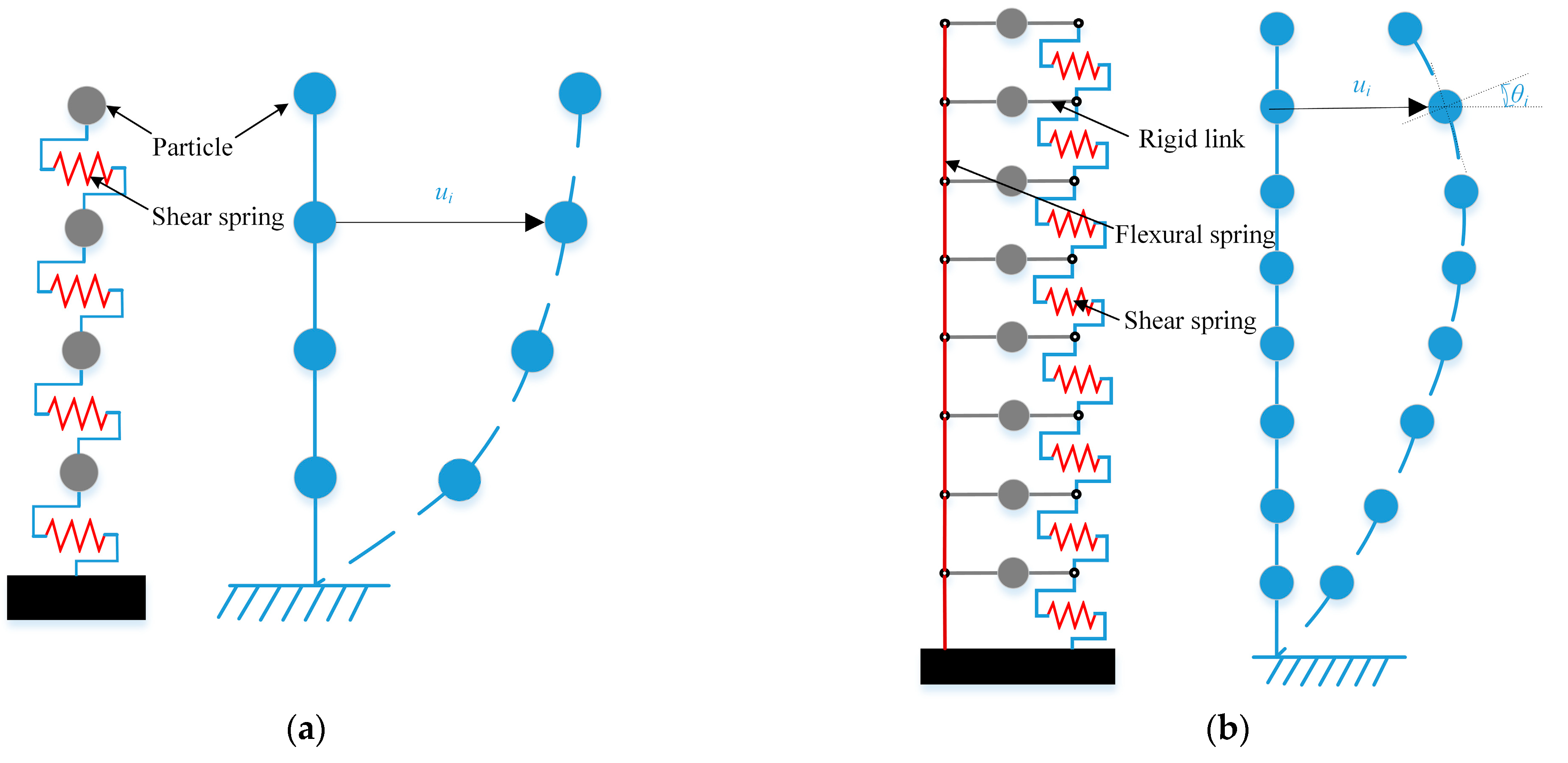
In the MDOF shear (Figure 1a) and flexural-shear models (Figure 1b) proposed by Xiong et al. [29,30], the backbone curve adopts the trilinear backbone curves model recommended by the HAZUS report (Figure 1c) and the single-parameter pinching model proposed by Steelman et al. [31] (Figure 1d) for the inter-story hysteresis model, which can better grasp the balance between the simulation accuracy and the difficulty of parameter calibration. The parameters that need to be calibrated for the MDOF model are elastic parameters, backbone curve parameters, and hysteresis parameters, among which, the elastic parameters of the shear model are the story mass m and shear stiffness , where m is obtained by multiplying the floor area with the empirical mass per unit area and is obtained by the empirical relationship between the story mass and stiffness and the structural self-resonance period; the elastic parameter of the flexural-shear model is the ratio of the flexural stiffness EI to the shear stiffness GA, , which is determined by the empirical formula of one and two cycles of the structure. The specific method for parameter calibration is detailed in the literature.
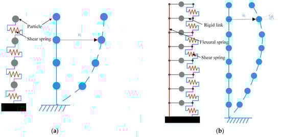
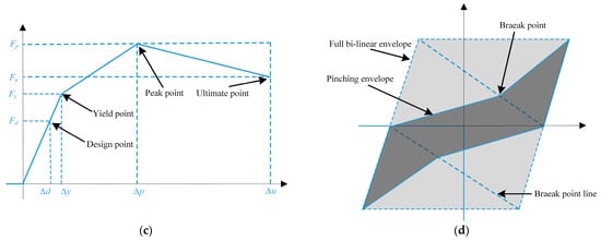
Figure 1.
(a) MDOF shear model; (b) MDOF flexural-shear model; (c) tri-linear backbone curve; and (d) single-parameter pinching model.
The structural arrangement of regional buildings is unknown and uncertain to the researcher at this point due to the frequent lack of structural information on buildings, and these structural design parameters determine the structure’s response under seismic excitation, as well as the resulting structural damage and economic losses. So, the design parameters that can express the characteristics of the structural arrangement of the building can be regarded as random variables, such as the type and strength of the material, the proportion, and the size of the components, etc., and simulate the actual structural design through the combination of a random sampling of multiple variables. Thus, the story mass m, the shear stiffness GA between stories, and the equivalent flexural stiffness EI of the shear walls are obtained from the component information to establish a simplified MDOF shear or flexural-shear structural analysis model. Multiple MDOF models are established for each building to consider the impacts of the uncertainty in the number of components and the design parameters on the seismic capacity of the structure and the seismic losses.
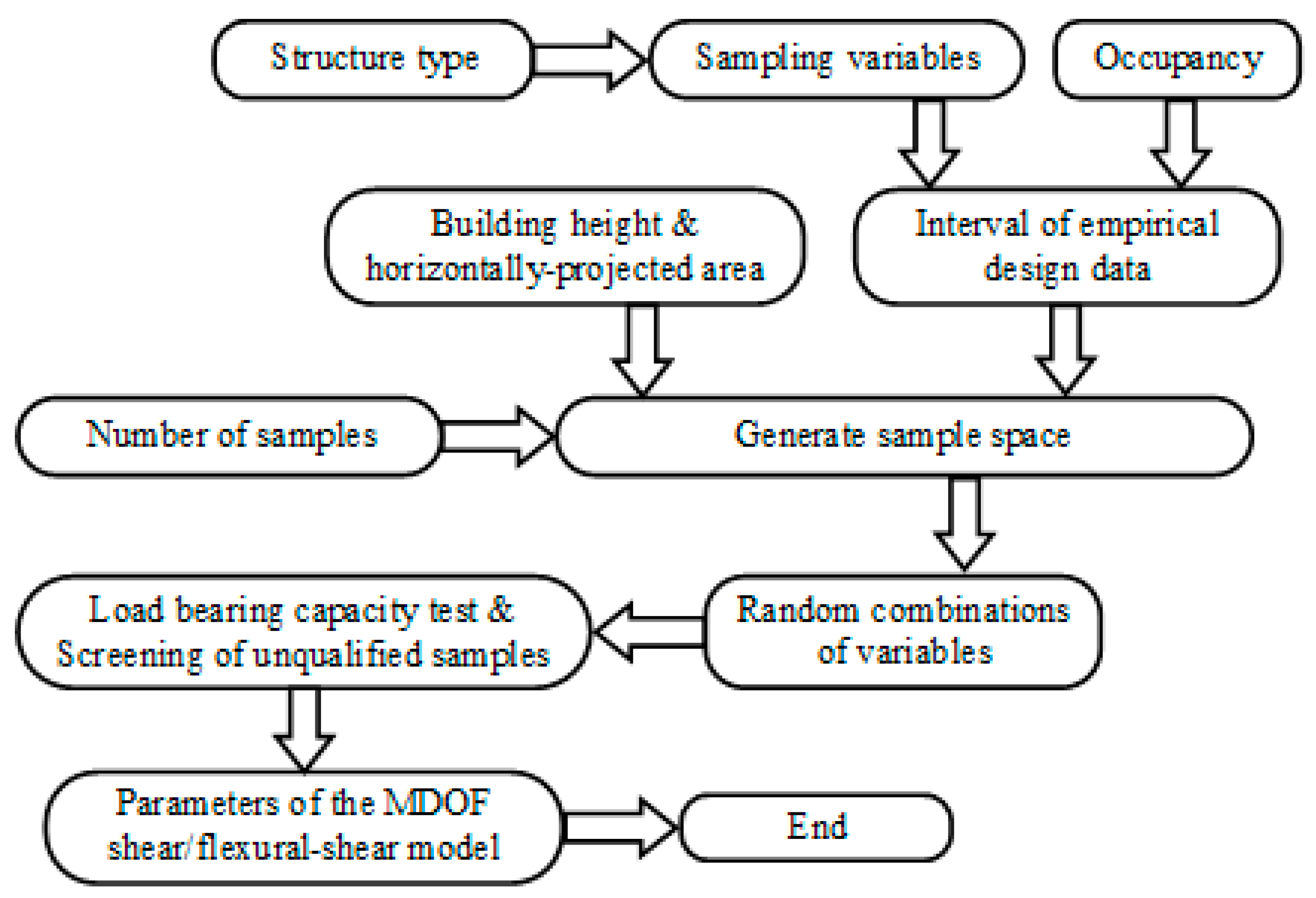
Benefiting from the development of remote sensing mapping technology, it is easy to obtain the appearance of the geometric parameters of a building, such as the building height and plane projection size, etc., through a geographic information system [13,25]. Therefore, it is possible to quickly obtain the basic information of each building through the GIS and take the rational design layout of the structure as the basic premise, based on the relevant norms and combined with the engineering experience of the typical architectural design. Based on the applicable codes and specific building design data from engineering experience, many story-based random structure samples are generated for each building and screened for verification. Finally, the MDOF shear/flexural model parameters, such as m, , GA, and EI, can be obtained from the SBRS model samples complying with the structural design codes, and the backbone curve parameters and hysteresis parameters are calibrated according to the methods proposed by Xiong et al. [29,30] and Steelman et al. [31], respectively. The process of the generation of the SBRS model samples is shown in Figure 2.
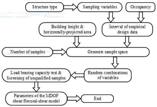
Figure 2.
The generation process of the SBRS model.
The SBRS model established in this paper represents the main structure of the building, including structural and non-structural components such as building columns, beams, slabs, and walls (shear walls and infill walls), etc. It does not include other appendages, such as electromechanical equipment, water supply, drainage systems, and decoration, etc. These factors are only considered in analyzing the structure’s mass and load-bearing capacity. In seismic response analysis, reinforced concrete is considered to be a macroscopic material based on its mass and material properties. The mass of masonry walls is obtained by multiplying the comprehensive bulk density and volume, considering the influence of mortar plastering. The plane and vertical structural arrangements of common civil building structures are generally more regular, and the boundaries between stories are clear, so the floor slabs of each story and the various types of components below them are assembled as a whole to establish the SBRS model, which is used as the basic structural analysis and calculation unit. To facilitate the research, this paper assumes that the structural arrangement of each story and component specifications are consistent.
2.2. Random Sampling Method
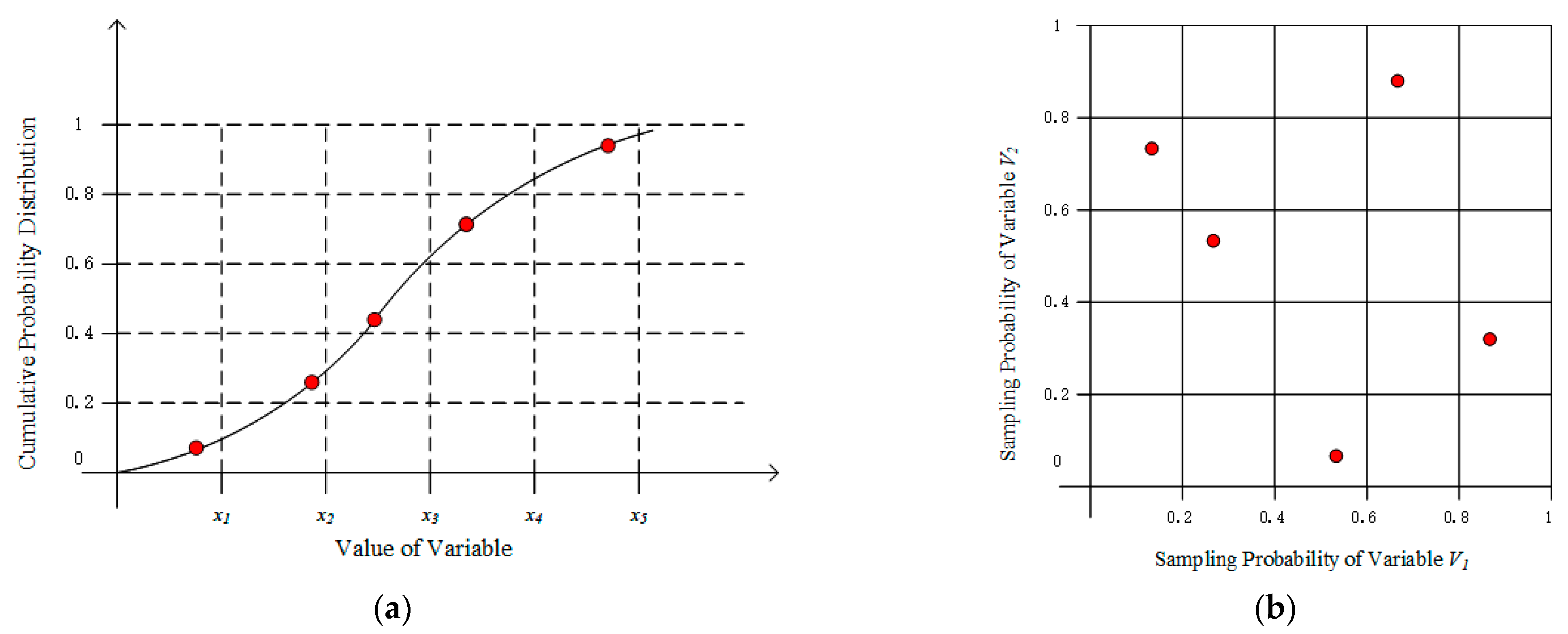
LHS is a method of approximate random sampling from multivariate distribution; the basic principle is equivocating each variable’s cumulative probability distribution into strata and selecting a sample in each stratum to recreate the probability distribution with fewer samples. The method has good stratified distribution properties, and a fully representative sample can be obtained by combining the sampled values of multiple variables in a randomly disordered order. If n denotes the desired number of sampling times and k denotes the number of random variables, the sampling space is k-dimensional. Then, an n × k matrix P is built, where each column is a set of 1, …, n random numbers in a chaotic order and is the n × k matrix consisting of independent random numbers obeying a uniform distribution from 0 to 1. As a result, the elements of the sampling matrix can be determined by Equation (1):
where is the inverse of the target cumulative distribution function and each row in now contains an input to the deterministic computation. For two input variables and five samples, the method principle and one possible sampling scheme are shown in Figure 3, the red dots indicate the samples obtained by random sampling.
Figure 3.
(a) Random stratified sampling of variables V1 and (b) random pairing of sampled V1 and V2.
The matrix P corresponding to it is:
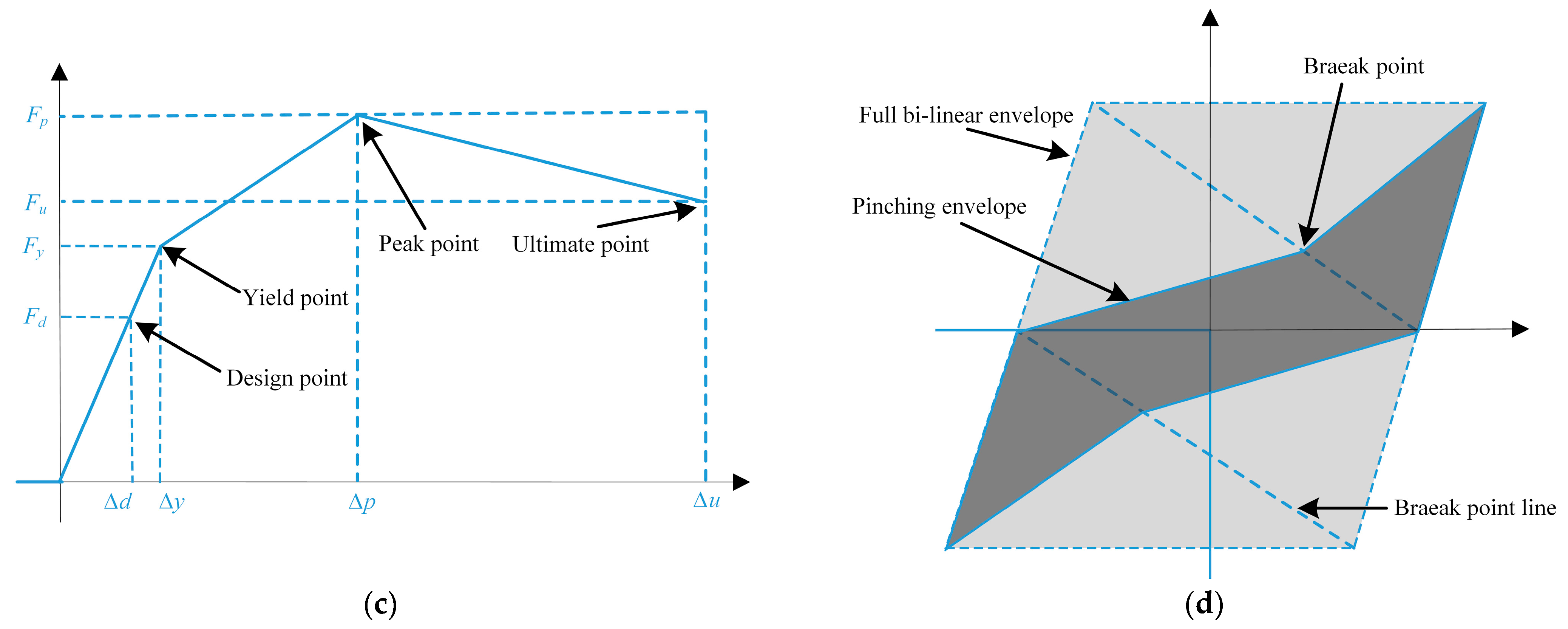
Compared with the Monte Carlo random sampling method, the LHS method has the advantages of a high sampling efficiency and strong sample representativeness with its memory sampling characteristics to avoid generating repeated samples, as shown in Figure 4. This paper utilizes the LHS method to randomly sample the structural variables, thereby improving the sampling efficiency and minimizing unnecessary computation, especially when the computational intensity is large when simulating the seismic response of the structure by using the dynamic time history analysis.
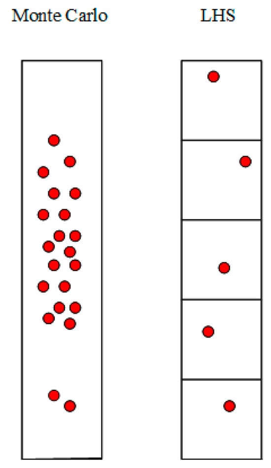
Figure 4.
Comparison between the Monte Carlo method and the LHS method.
2.3. Methods for Building the Sample Space
The design parameters that can express the characteristics of the structural arrangement mainly include two categories: component size and material type. No research conclusion can be referred to for the probability distribution form of the selected random sampling variables. However, if the expectation and the variance of a random variable X, then for different values of the vector , when n is large enough (the sample size of 30 is generally considered to be sufficient), the mean value of will approximately obey a normal distribution, denoted as , as shown in Equation (3).
Equation (3) is known as the Central Limit Theorem (CLT), that is, regardless of the distribution of a set of random variables to obey what form (except the Cauchy distribution), when a random sample of mutually independent data is taken from it, the number of samples collected is sufficiently large (it is generally considered that the number of samples can be up to 30), and this group of variables will converge to the normal distribution of the sample mean.
In other words, for the selected randomly sampled variables, regardless of the form of distribution to which they are subjected, the sample mean will be distributed near the overall standard of the variable and will be normally distributed. Common civil buildings generally follow the safe and economical design concept, and there will be empirical design parameters in the reference range in engineering practice. When the probability distribution form of the variable cannot be determined, combining the engineering experience with the design data for each sampling variable to select the appropriate intervals, so that the interval can cover the overall mean value of the variable, and assuming that it is approximately obeys the uniform distribution within the interval are consistent with the engineering practice. By analyzing the statistics of many samples, its sample mean value can better reflect the expected earthquake loss of the actual structure.
For a random variable obeying a uniform distribution, the inverse cumulative distribution function is:
where a and b denote the boundaries of the values of the random variables and p is the cumulative distribution probability.
The random variables of the SBRS model can be categorized into two types: discrete and continuous. For discrete variables, the probability intervals in which the variables take values correspond directly to the random numbers generated by the MATLAB program, drawing on the random sampling methodology used in FEMA-P58 to determine the damage state of a member. For example, for the random variable of the frame column cross-sectional area, first, the probability (in percentile) that each type of cross-section occurs in the sample space is determined, and since the sum of the probabilities should be 1, the probability intervals corresponding to each type can be determined; then, random numbers from 1 to 100 are generated for each sample, with the value of each random number representing the percentile value of the probability, and the probability intervals that the random numbers are in are generated, which represent the random sampling results for that cross-sectional area.
The variable value interval is first divided into equal proportions for the continuous type sampling variable. The total number of interval nodes is the same as the number of random samples to be generated. Then, the value of each interval node corresponds to the random number, and the formula for the value of the continuous type random variable can be obtained from Equations (3) and (4), as shown in Equation (5):
where is the lower limit of the value interval, is the upper limit, N is the number of samples, and i is the generated random number, an integer no larger than N.
The higher the number of random structural samples, the greater the possibility of generating samples similar to the actual structural arrangement, but due to the existence of marginal effects, the efficiency of the loss sample means to approach the loss expectation gradually decreases with an increase in the number of samples. This will greatly increase the computational workload.
For reinforced masonry (RM) structures and RC frame structures, the dynamic characteristics of the structure tend to be stable after the number of samples reaches 60. The RC frame shear structure requires about 40 samples. According to the bearing capacity analysis of the SBRS model, the passing rate of RC frame structures is generally around 70%. In contrast, RM structures and RC wall-frame structures with less than 10 stories are qualified, while the passing rate of RC wall-frame structures decreases with an increase in the number of stories, and the passing rate is around 50% when the number of floors is more than 30. The initial sample size of all SBRS models in this paper is 100, which can better balance the accuracy of the loss averages with the computational efficiency and can also meet the requirements of the CLT theorem for the number of sampling times.
3. SBRS Model Sampling Process
3.1. Treatment of Building Plan
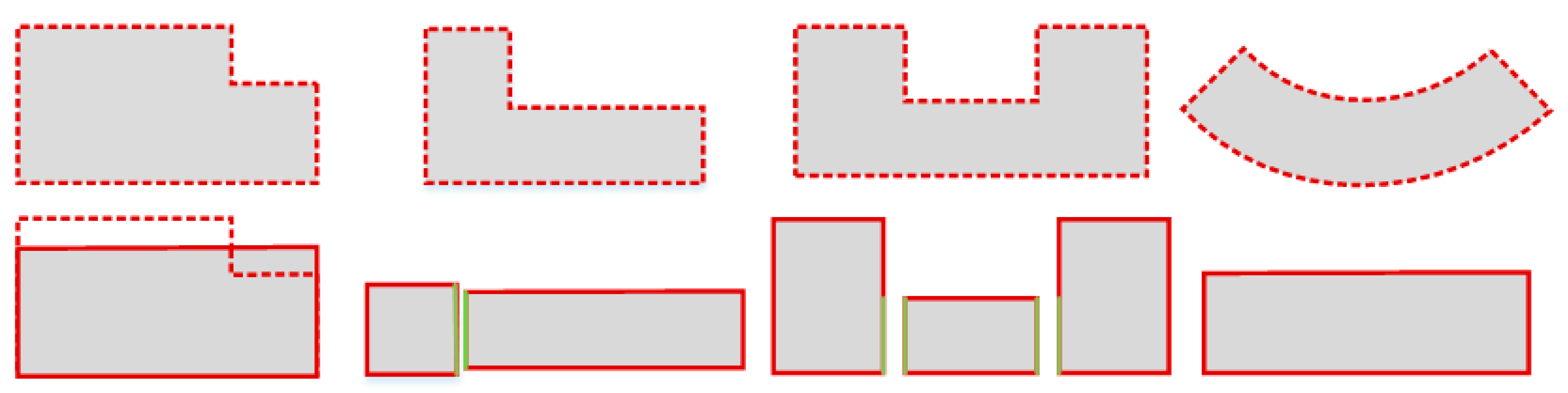
Most building planes are more regular rectangles or near-rectangles. According to the provisions of GB 50011-2010, the Code for Seismic Design of Buildings [32], when the dimensions of the plane concavity are greater than 30% of the total dimensions of the corresponding projection direction, this is a concave-convex irregularity. For buildings with non-standard rectangular planes that exist in actual projects, they are handled in the following ways:
- (1)
- For buildings where the concave dimension of the plane does not exceed 30% of the total size of the corresponding projection direction, the plane is equivalently reconstructed as a regular rectangle equal to its area [33].
- (2)
- When the plane is concave by more than 30%, the layout form of the internal structure and the number of components are estimated, respectively, and summarized after removing the overlapped parts.
- (3)
- For curved buildings, they are equivalently reconfigured as equal-area rectangles of the same width.
As shown in Figure 5, the dotted plane is the original plan outline of the building, and the red and green solid lines are the equivalent reconstruction planes and overlap lines.
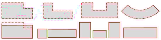
Figure 5.
Equivalent reconstruction of building plane.
3.2. Common Layout for Structures
RC frame structures, RC wall-frame structures, and reinforced masonry structures account for many service structures. The layout of the RC frame structure is relatively simple; the key lies in the arrangement of the column network, and the structure is dominated by shear deformation under the effect of an earthquake, while the RC wall-frame structure combines the characteristics of the two structural systems of the frame and shear wall. The shear wall system is dominated by bending deformation. Shear walls and frame columns are the main lateral force-resisting members, and the former usually serves as the first line of defense against seismic effects. When encountering small seismic effects, shear walls exhibit bending deformation to consume seismic energy; when encountering large seismic intensity, the attached beams and the bottom of the limbs of the shear walls are the first to be damaged, and the frame columns serve as the second line of defense, which play a role in the redistribution of the structural plastic internal forces. Therefore, the total cross-section of the lateral-resisting members on each story of a reasonably designed RC wall-frame structure is kept within a certain range from the floor area, as shown in Table 1, where , , and are the cross-sectional area of shear walls, the cross-sectional area of framing columns, and the floor plane area, respectively.

Table 1.
The ratio of the cross-sectional area of the lateral force-resisting components to the floor area.
The shear wall arrangement should generally follow the following principles in the design of wall-frame structures:
- (1)
- Shear walls should be arranged bi-directionally along the main axis of the building, and both should have a similar total lateral stiffness.
- (2)
- Shear walls should be evenly distributed in the floor plane, and the spacing should be manageable to ensure that the building cover has sufficient stiffness in its plane.
- (3)
- For a regular rectangular floor plan, the shear wall should be suitable to maintain basic symmetry along the longitudinal and transverse bi-directional plane centerline.
- (4)
- Shear walls should be set through the entire building height to avoid sudden changes in stiffness to form a weak structure story.
- (5)
- The cross-section of the shear wall should be simple and regular to avoid the appearance of a complex and shaped cross-section.
- (6)
- The ratio of the total height of the shear wall to its section height should be at least 3, and the section height of the wall limb should generally not be more than 8 m.
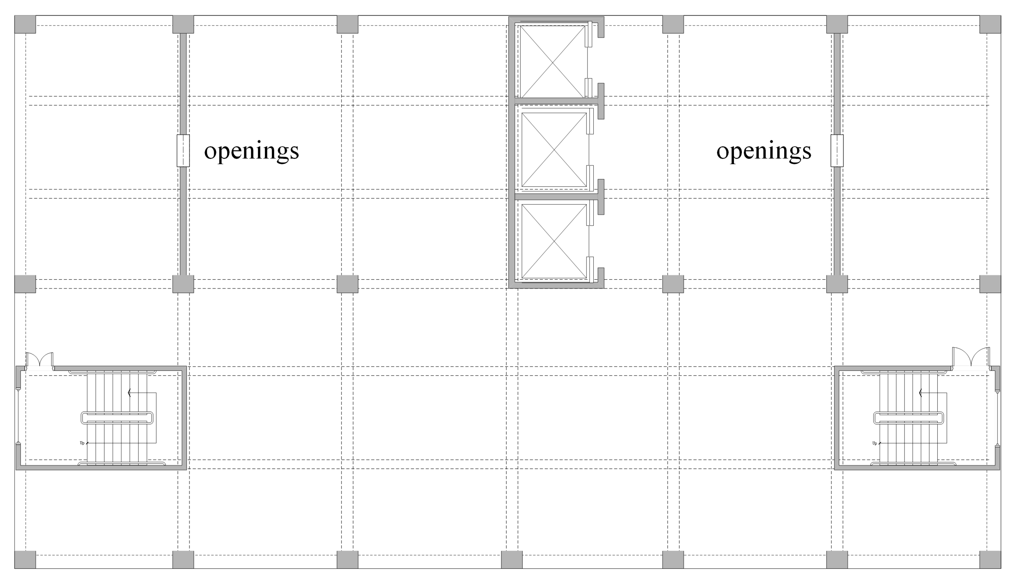
The shear wall serves as a vertical load and resists lateral forces in the building structure. Furthermore, it demarcates and encloses distinct spaces within the building. High-rise wall-frame structures are usually combined with stairwells, elevator shafts, and other vertical access arrangements in the local formation of a relatively large stiffness of the approximate cylindrical structure, with the distribution of other parts of the building wall limbs to jointly resist seismic effects, wind loads, and other lateral forces. A wall-frame-structured office building is being referred to, with an example of a common layout shown in Figure 6. The gray-shaded portions of the frame columns and shear walls in the middle of the long limb shear wall can be opened according to the need for door openings; the dotted line part of the frame beams, secondary beams, and infill walls are not shown in the figure.
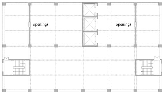
Figure 6.
Plan of office building of wall-frame structure.
Reinforced masonry structures mainly show shear-type damage under the effect of earthquakes, and according to the different ways of vertical load transfer and load-bearing walls, they can usually be divided into three kinds of load-bearing methods: transverse wall bearing, longitudinal wall bearing, and longitudinal and transverse wall joint bearing. Because the wall of a reinforced masonry structure has space separation and structural load-bearing functions, its internal layout is complex and variable, and it is challenging to judge the specific structural arrangement accurately. However, the lateral resistance of reinforced masonry structures mainly comes from the load-bearing wall; material strength, wall section length, and wall thickness are the main factors affecting the shear stiffness of the wall. Seismic performance analysis only needs to clarify the cross-sectional area of the internal seismic wall.
According to the statistics of Su et al. [34] on a large number of masonry structure earthquake-damaged houses in the Wenchuan earthquake, the ratio of the cross-sectional area of longitudinal to transversal walls of each story to the floor area (excluding the balcony) was from 13% to 15%. The ratio of the cross-sectional area of load-bearing walls to the floor area was about 9%. The ratio of the cross-sectional area of structural columns to the floor area was generally 0.3~0.4% for earlier ones and 0.5~0.7% for newer ones, which is more in line with the 0.3~0.6% measured by the author according to the GB 50011-2010 [32].
3.3. Generate the SBRS Model
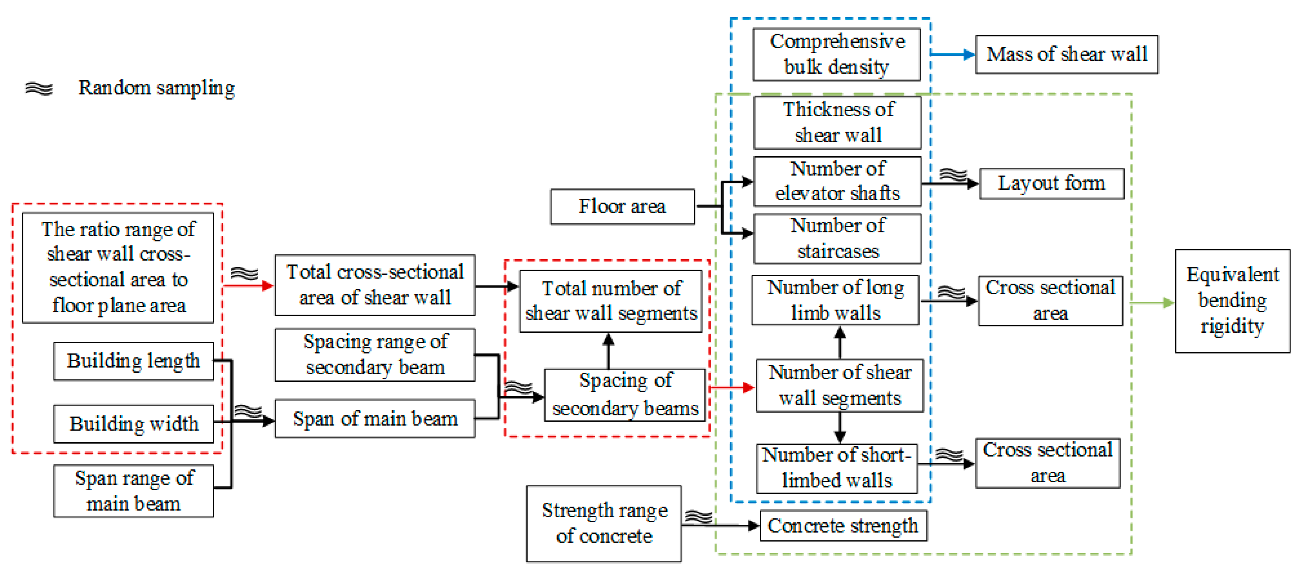
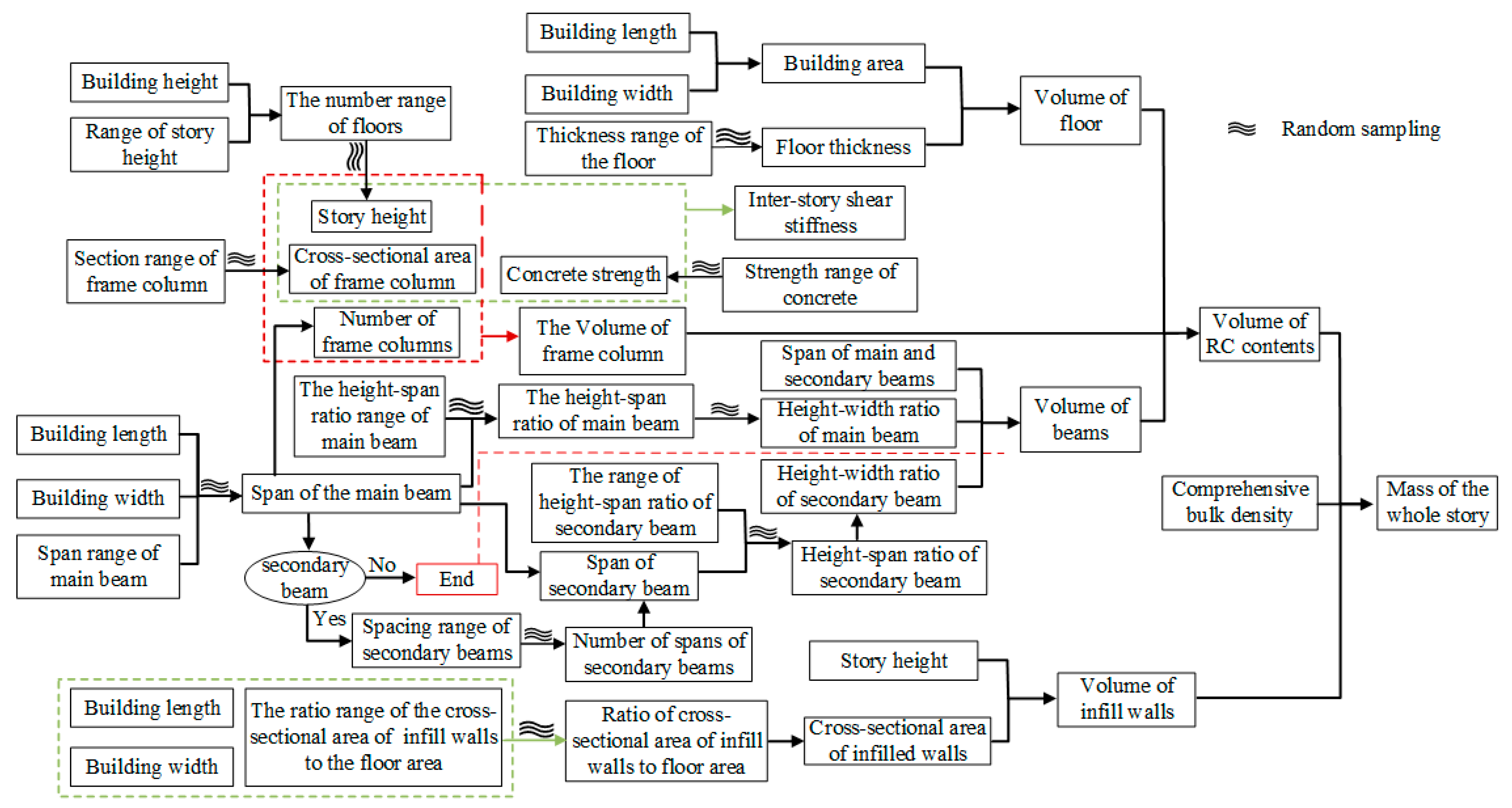
To generate Seismic Building Response Simulation (SBRS) models, the first step is to obtain the building’s basic information, such as its structural type, occupancy, plan area, and construction time. The plane contour of the building is used as the boundary constraint, and the column spacing and beam span are speculated based on engineering experience. These are then combined randomly with parameters such as component size and material strength to form several groups of design parameters that can establish a physical model. Through the statistics of a number of various types of components, the lateral stiffness of the structure and the mass of each story, seismic response, damage assessment, and loss estimation can be carried out. Figure 7 shows a sketch of the generation process of SBRS models.
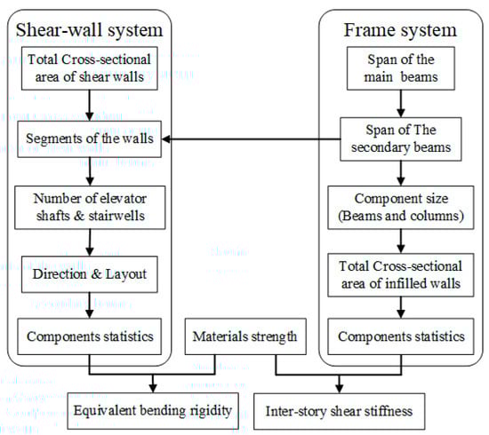
Figure 7.
Sketch of the generation process of SBRS models.
According to the layout characteristics of the wall-frame structure, the following assumptions can be made for the calculation of the shear wall cross-sectional area and the judgment of the number of wall sections:
- (1)
- The spacing of secondary beams is the basic unit of measurement of shear wall section height, and the number of wall segments is obtained based on the total cross-sectional area of the shear wall. Usually, the number of wall segments obtained from the calculation is partial. After rounding up, the total shear wall section height in the direction of the short side of the building is slightly larger than that in the direction of the long side.
- (2)
- After deducting the total number of shear wall sections in the direction of the short side of the building from the elevator shafts and stairwells, this is divided by the spacing of the framing columns on the short side of the building to obtain the number of long sections of shear walls; if it is not possible to divide the whole number, the spacing of the secondary beams is used as the height of the section to obtain the number of remaining wall sections.
- (3)
- The direction of the short side of the building is the seismically unfavorable direction, and the cross-sectional area and equivalent bending stiffness of the shear wall in that direction are calculated.
- (4)
- Except for connecting beams in elevator shafts, stairwells, and long sections of shear wall openings, the number of connecting beams between shear walls is determined by random sampling. If the number of shear walls is N, the upper limit of the number of connecting beams is N − 1.
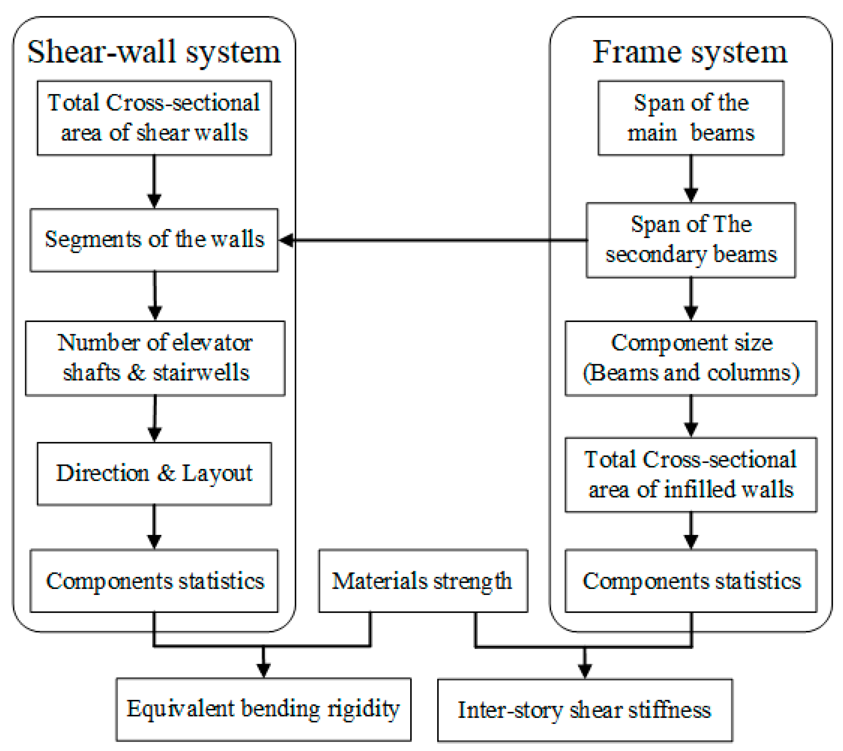
In summary, for the wall-frame structure SBRS model, the flow of establishing a shear wall system is shown in Figure 8.
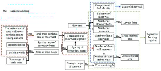
Figure 8.
Establishment process of the shear wall system of the SBRS model.
The establishment of the frame system mainly lies in the arrangement of the column network, and the establishment process is shown in Figure 9.
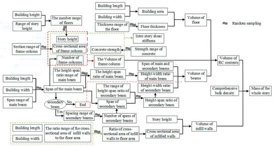
Figure 9.
Establishment process of frame system of SBRS model.
The sampling variables required for wall-frame structures are shown in Table 2. The data presented in the sample values are the results of sampling the random variables of one SBRS model in the case study, and the process and the distribution parameters of variables are described in Section 3.2.
Table 2.
Types of random sampling variables for wall-frame structure SBRS models.
Reinforced masonry structures can be modeled using a similar process to that used to build the SBRS model for RC frame structures shown in Figure 6, where the ratio of the cross-sectional area of the infill wall to the floor area is replaced with the ratio of the cross-sectional area of the load-bearing wall to the floor area. Then, variables such as the strength of the block and mortar are selected for a combination of random sampling to obtain an SBRS model that meets the universal design characteristics, which will not be repeated here.
4. Case Study
4.1. Basic Information on Regional Buildings
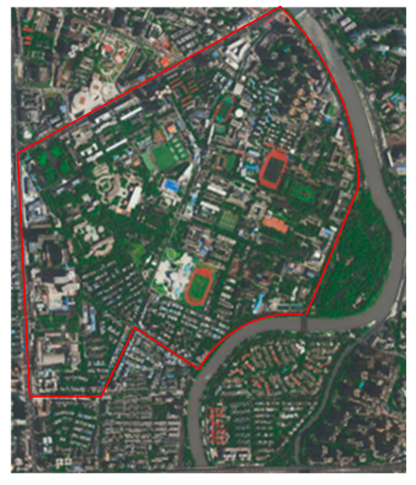
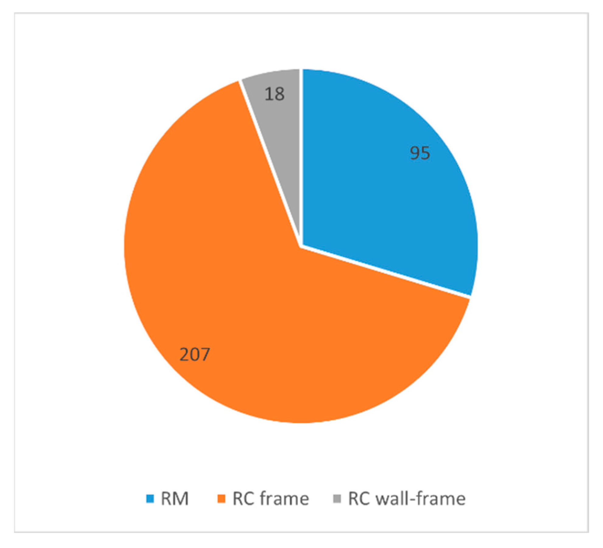
Taking the Wangjiang Campus of Sichuan University in Southwest China as an example, the proposed SBRS modeling method and how to adopt the SBRS models to estimate the earthquake loss of regional buildings are elaborated in detail. The site type where the campus is located is Site II; the seismic intensity is 7 degrees and the design seismic basic acceleration is 0.1 g. The Gaode live map of the campus is shown in Figure 10. There are 320 buildings on the campus, and their number ratio and distribution in geospatial space are shown in Figure 11 and Figure 12, respectively.
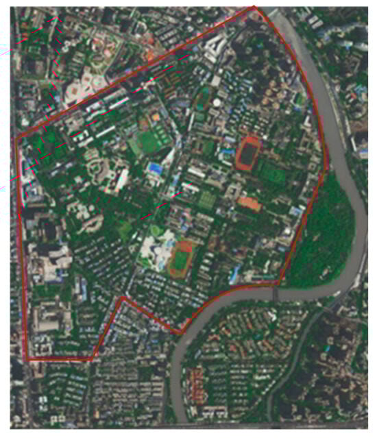
Figure 10.
Gaode real map of the campus.

Figure 11.
The proportion of structural types.
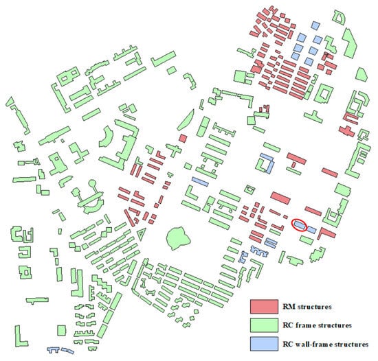
Figure 12.
Spatial distribution of building structure types on Wangjiang campus. The red circle indicates the study area of this paper.
4.2. SBRS Models Generation
Based on the building vector information obtained from the open-data platform of Gaode Map, the 3D information model containing the spatial location information is converted and outputted through the data interface of GIS, which can obtain the geometrical information of the building appearance with a high efficiency [25]. Taking the wall-frame structure office building boxed by the red circle in Figure 9 as an example, the lengths of each side transformed from the coordinate point data acquired by GIS are 18.8204 m, 45.6020 m, 18.8201 m, and 45.6029 m, respectively, and the adjusted long side of the building is taken to be 45.6 m, the short side to be 18.8 m, and the height to be 26.4 m. The ranges of values of the parameters of the SBRS model are as follows:
- (1)
- Story height. The story heights of office buildings are generally in the range from 3.0 to 3.6 m.
- (2)
- Bidirectional main and secondary beam spans. The main beam’s span range in the building’s short side direction is usually from 6 to 8 m, the long side direction is from 4 to 6 m, and the secondary beams are laid out at spacings from 2 to 3 m.
- (3)
- The cross-sectional area of the frame column. It can be assumed that the square columns have side lengths ranging from 600 to 800 mm, with 50 mm as the basic unit of increase or decrease.
- (4)
- Material strength. The concrete strength grade is C30~C40, and the thickness of the infill wall is uniformly taken at 200 mm. The ratio of the cross-section to the floor plane is taken as 5~8% according to engineering experience. According to GB 11968-2020, the Standard for Autoclaved Aerated Concrete Blocks [35], the commonly used grade markings for autoclaved aerated concrete blocks are B05 and B06. The corresponding dry weights are 500 kg/m3 and 600 kg/m3, considering mortar, plaster, and other factors, and the integrated volume weight is 900 kg/m3.
- (5)
- Shear wall section size. The shear wall thickness is 200 mm, and the ratio of the shear wall cross-sectional area to the floor area is from 2% to 3%; for office buildings, in addition to stairwells and elevator shafts outside, the other shear wall section is simplified to take the “I” type column–wall combination section.
- (6)
- Number of stairwells and elevator shafts. According to the building area, two sets of evacuation stairs should be set up to meet the requirement that the straight distance to the evacuation door between the two safety exits is not less than 40 m in the Code for Fire Protection Design of Buildings [36]. According to the floor area projection of three elevators, the short side of the building, in the direction of the main beam span range, meets the unilateral layout of the space requirements.
- (7)
- Other parameters. According to the provisions of Article 3.1.1 of GB 50009-2012, the Load code for the design of building structures [37], the loads of the building structure are divided into three categories: permanent load, variable load, and accidental load, and only the first two categories are considered in this paper. Among them, the constant loads such as fixed equipment and long-term storage outside the building body are considered as 1.1 times the load of the building body, and for variable loads, standard, combined, frequent, or quasi-permanent values should be used as representative values according to the design requirements. The standard value of floor distributed live load is 2.0 kN/m2, the combination value coefficient is 0.7, the frequency value coefficient is 0.5, the coefficient of live load reduction according to the stories is 0.65, and the structural damping ratio is 0.05.
Assuming that each of the aforementioned random variables follows a uniform distribution across their respective value ranges, the LHS method randomly combines the selected variables to generate 100 SBRS models and perform axial compression ratio checking to screen out the unqualified samples. According to the GB 50011-2010 [32], the limit value of the axial compression ratio for RC wall-frame structures is 0.90. All the models in this case meet the load-carrying capacity requirements, and the values of the parameters of each sampling variable for one of the randomly selected models are shown in Table 3.
Table 3.
Parameter statistics of RC wall-frame SBRS model.
After several sample simulation generation tests with a model number of 100, the generated SBRS models occasionally have samples that do not meet the axial compression ratio limit of up to 3. The main reason for this is that the building height is small, the total number of stories is only 8, and the first story of the vertical load-bearing contents can meet the load-bearing requirements. With an increase in the number of stories, the passing rate of the models gradually decreases, and for the buildings with more than 30 stories, the passing rate of the SBRS models is around 50%. Therefore, when modeling higher buildings, consideration should be given to appropriately increasing the cross-sectional area of columns and improving the concrete strength grade to ensure the pass rate of the models.
In addition, the quality of the models can be examined by λ, the stiffness eigenvalue which can reflect the ratio of the total stiffness of the frame to the shear wall, as shown in Equation (6):
where H is the building height. When the stiffness eigenvalue (λ) of the RC wall-frame structure is too small, the structural plastic internal force redistribution that occurs after the destruction of the shear wall system can make it difficult for the frame system to resist seismic activity. This can lead to the immediate failure of the structural system. Conversely, when λ is too large, the frame beams are damaged at the bottom of the wall limb first. A large number of the frame beams being damaged at the end of the beams can lead to columns appearing in plastic hinges. This can cause the structure to fail or collapse, and the desired seismic performance cannot be achieved. Only when the stiffness eigenvalue is within the appropriate range can the RC wall-frame structure achieve the ideal damage mode of “shear wall system first and then the frame system”.
The stiffness eigenvalues of wall-frame structures are recommended to be 1.15 ≤ λ ≤ 2.4 in the Concise High-Rise Reinforced Concrete Structural Design Manual [38]. The models are more consistent with the recommended range of values, indicating that the SBRS model established by this method can realize the original design intention of the double line of defense for the shear wall and frame systems. The differences in the inter-story shear stiffness GA, the equivalent flexural stiffness EI, stiffness eigenvalue λ, and story mass m differences between the samples are statistically shown in Table 3.
Since RC frame and reinforced masonry structures are both low-rise and multi-story buildings, the SBRS models generated for buildings of these two types of structures on the campus can meet the load-bearing capacity requirements. Occasionally, individual SBRS models of RC frame structures need to meet the load-bearing capacity requirements, mainly due to the coupling of larger spans, smaller column cross-sections, and lower concrete strengths.
4.3. Earthquake Loss of Single Buildings
The SBRS model is mainly used for the loss estimation of buildings under different ground shaking effects from a regional buildings perspective rather than selecting ground motion records that match the target design spectrum based on the principle of the most unfavorable set of defenses from the seismic design perspective, thus using a site condition-based wave selection. According to Vamvatsikos et al. [39], 20 ground motion records inputted in an IDA analysis are sufficient to respond to the uncertainty of ground shaking, and 22 ground motion records from the FEMA-P695 report [40] with a shear wave velocity similar to the site condition are selected. The modulation step is taken to be 0.1 g. Due to the large number of buildings in the area and the significant difference in the fundamental period, the preferred method for determining ground shaking intensity is Peak Ground Acceleration (PGA). Subsequently, the selected ground motion records are inputted into the model for Incremental Dynamic Analysis (IDA) analysis.
Assuming that m ground motion records are inputted at each intensity for each SBRS model, the seismic demand parameter EDP of each story can be formed into an m × 1 vector and the EDP of each story of the n models is an m × n matrix, with each element value denoted as . The median value of the fetched vector is taken as a representative of that model’s value, denoted as . Therefore, for all models, can be composed of a 1 × n vector, and the median value of this vector is used as the representative value of the peak inter-story displacement of each story of the building, denoted as . When the amplitude-modulation step is 0.1 g, the change in the seismic response is more stable between the steps, and due to the excellent seismic performance of the wall-frame structure, the seismic response still does not reach the limit value of collapse when PGA = 1.0 g. Considering that there are few seismic events with PGA reaching 1.0 g, to improve the computational efficiency, we did not continue to increase the intensity of the inputted ground shaking until most of the models collapsed and stopped the process of the IDA computation at PGA = 1.0 g.
The damage state of structures is usually defined by discrete damage states, such as HAZUS, Vision 2000 [41], EMS-98 [42], and the China specification GB/T 24335-2009, the Classification of Earthquake Damage to Buildings and Special Structures [43], which classifies the damage state of buildings as Intact, Slight, Moderate, Severe, and Complete. China’s seismic code defines the elastic limit and plastic limit of a structure using 1/550 and 1/50 of the inter-story drift ratios, respectively [32]. On the other hand, 1%, 2%, and 4% are used to define the limit states of immediate occupancy, life safety, and collapse prevention [44], so the inter-story drift ratio intervals for each damage state used in this paper are shown in Table 4.
Table 4.
Inter-story drift ratios corresponding to each damage state.
For each damage state of the structures, the type, number, and damage degree of components are determined based on their respective damage state definitions. Since the number of damaged contents is an interval value, the linear interpolation method can be used to determine the ratio of the number of damaged contents according to the seismic response of the structure. Then, according to the damage degree of the contents, JGJIT415-2017, the Technical Specification for Post-Earthquake Urgent Assessment and Repair of Buildings [45], is referred to and combined with the cost documents to determine the loss ratio of each type of content, i.e., the ratio of the cost required to restore a component with a certain damage degree to its pre-earthquake state to the replacement cost of that component, as shown in Table 5.
Table 5.
Loss ratios of components corresponding to each damage degree.
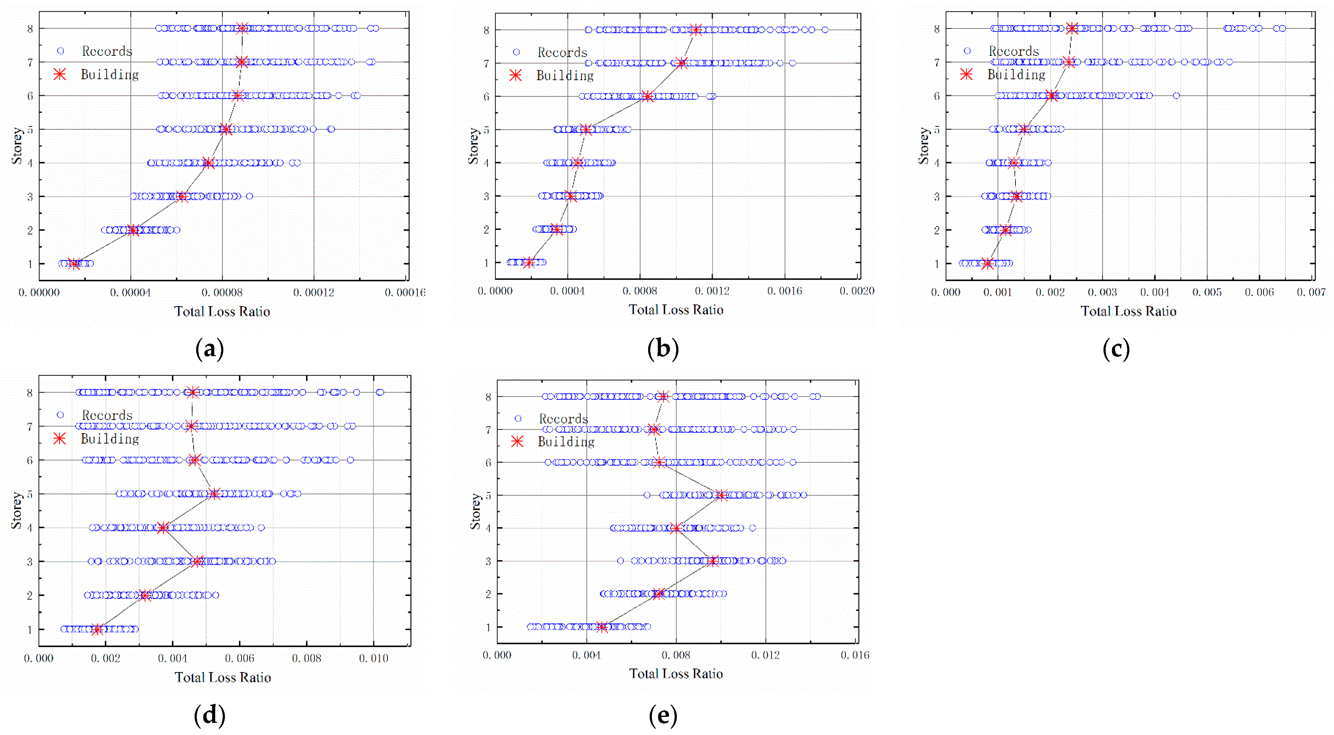
Based on the construction cost statistics of RC buildings, a deterministic cost contribution of each type of component is used [20], which was developed by using the mean square foot costs of reinforced structures and engineering judgment. By analyzing the damage state of each story in different SBRS models, we can determine the loss ratio of each story. Since it is assumed that the construction of each story is the same, we can calculate the total loss ratio (TRL) of the building. The TRL in this paper is the loss to the superstructure building cost, which does not include services and substructures. We can then multiply the total loss ratio by the unit construction cost and building area to determine the earthquake loss of the building. The and values of the loss ratios for each story are shown in Figure 13. As we move from the bottom to the top of the story, it becomes evident that the loss distribution for all SBRS models increases gradually. The data dispersion between different models increases gradually, with the most noticeable difference being in the upper stories.
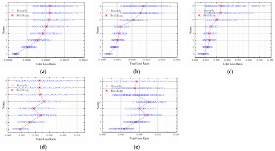
Figure 13.
and of loss ratio for each story: (a) PGA = 0.1 g; (b) PGA = 0.3 g; (c) PGA = 0.5 g; (d) PGA = 0.7 g; and (e) PGA = 0.9 g.
It is commonly assumed that, under equal ground motion intensity, a building’s earthquake losses follow a lognormal distribution [17]. Therefore, the median value of the building’s total loss ratio (represented by ) correlates with the ground motion intensity via a power–exponential relationship, as outlined in Equation (7):
where is the median value of the building earthquake loss ratio, and a and b are regression coefficients. Taking logarithms on both sides of Equation (8):
where and b can be obtained by regressing earthquake loss data. By fitting the loss ratios to all models, the probability curve of earthquake losses and the log standard deviation can be obtained:
where N is the number of fitted data.
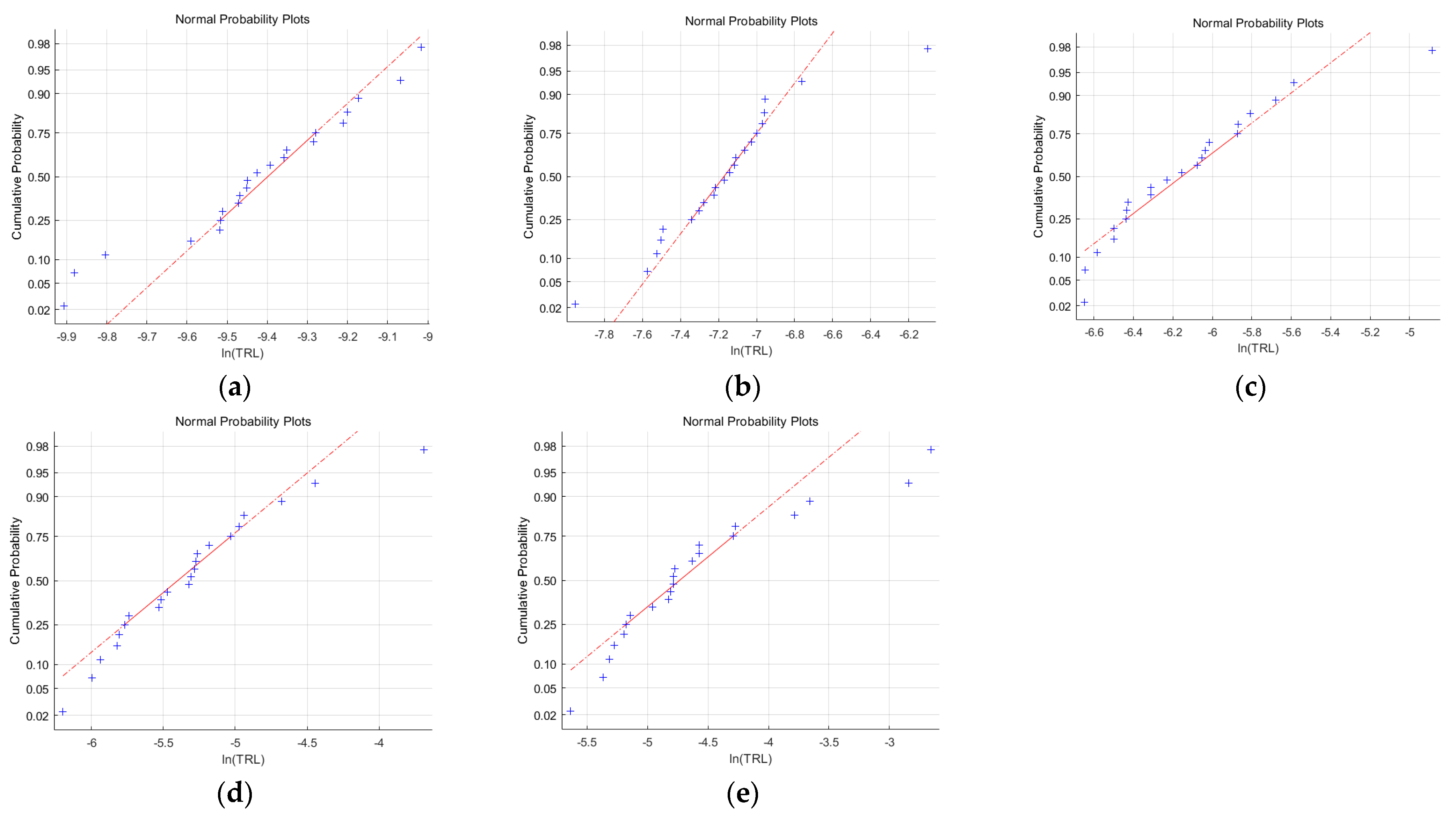
The logarithmic value of the total loss ratio was tested for normal distribution using Kolmogorov-Smirnov test. The loss ratio of individual SBRS models was first validated with the model in Table 3, and the confidence level was 5%. The fitting results are shown in Figure 14, where the x-axis value is the ith logarithmic total loss ratio of the model sorted from low to high, and the y-axis represents the quantiles of the normal distribution converted into probability values. The results show that, for all ground motion intensities, the test results agree to obey the original hypothesis, i.e., the total loss ratio of a single model obeys a lognormal distribution under different ground motion intensities.
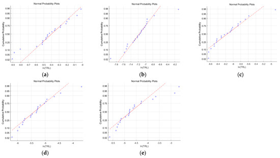
Figure 14.
Log−normal distribution fit of the total loss ratio for a single model: (a) PGA = 0.1 g; (b) PGA = 0.3 g; (c) PGA = 0.5 g; (d) PGA = 0.7 g; and (e) PGA = 0.9 g.
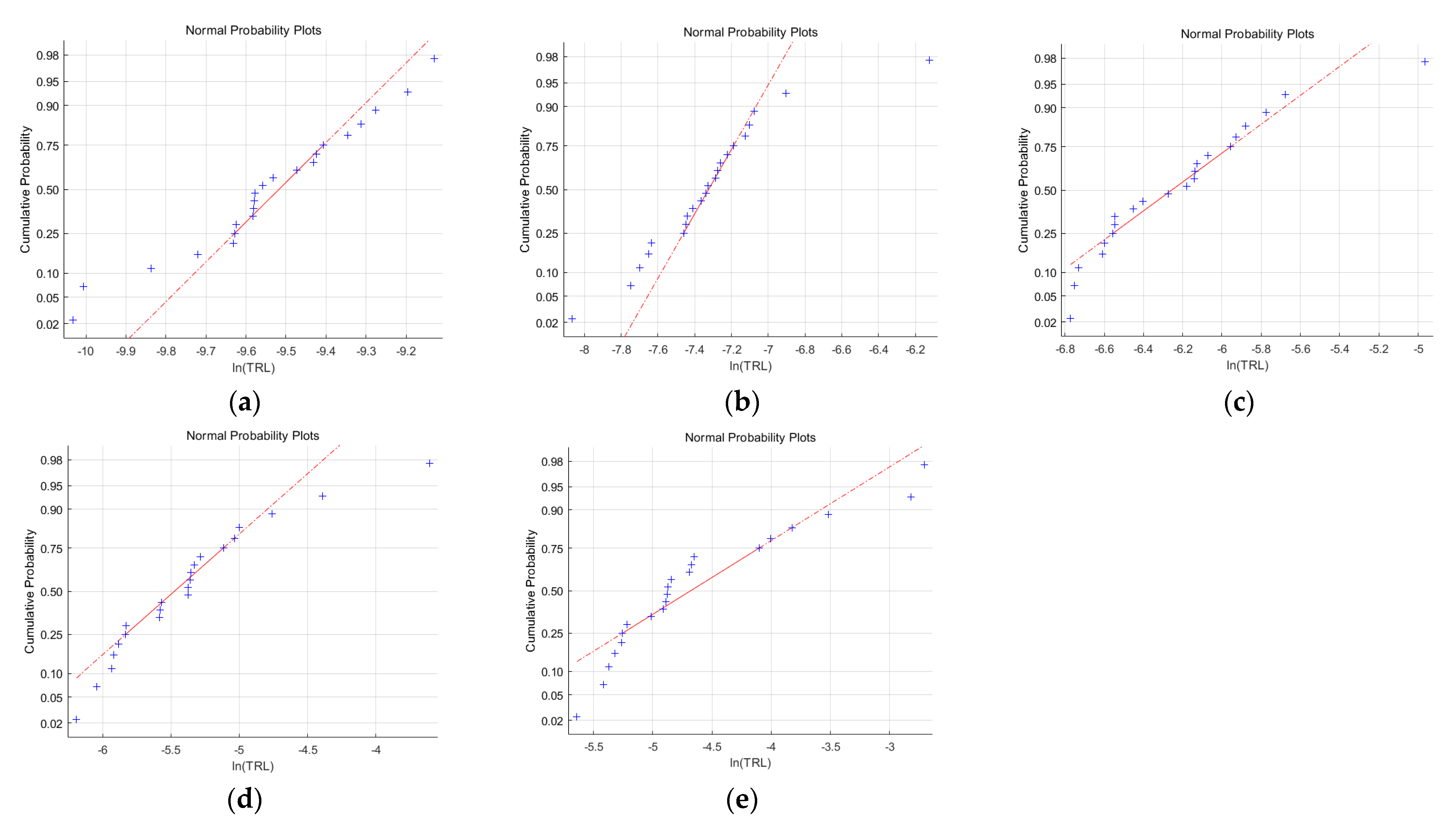
For each ground motion record, the median value of the total loss ratio of the SBRS models is taken as the representative value of for that ground motion record. This vector value measures the variability among models from the perspective of all the models, and the 22 values of the loss ratio are examined. The fitting results are shown in Figure 15, which the blue ’ + ’ symbol are the data points, and the red line is the fitting line. The results show that, as with the test for a single random sample, the values for the structure obey a lognormal distribution for all calculated ground motion intensities. Upon comparison, it is observed that there is a high degree of similarity between the loss ratio of a single SBRS model and the distribution trend of the sample value, denoted by , under different seismic intensities of the fitted data. This similarity serves as evidence for the reasonableness of the sample value as a representative value for different samples, which can effectively account for their variability.
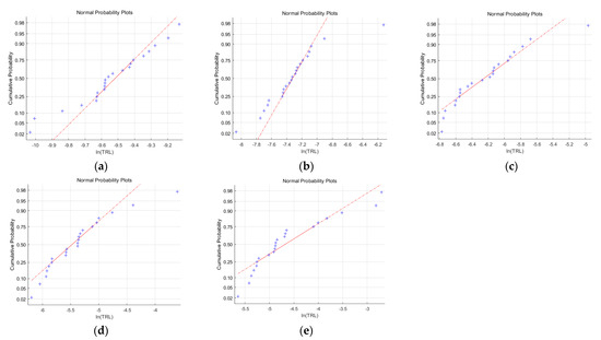
Figure 15.
Log−normal distribution fit of total loss ratio of values: (a) PGA = 0.1 g; (b) PGA = 0.3 g; (c) PGA = 0.5 g; (d) PGA = 0.7 g; and (e) PGA = 0.9 g.
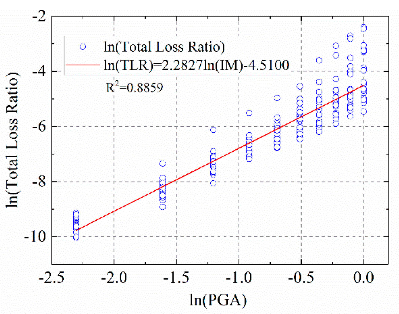
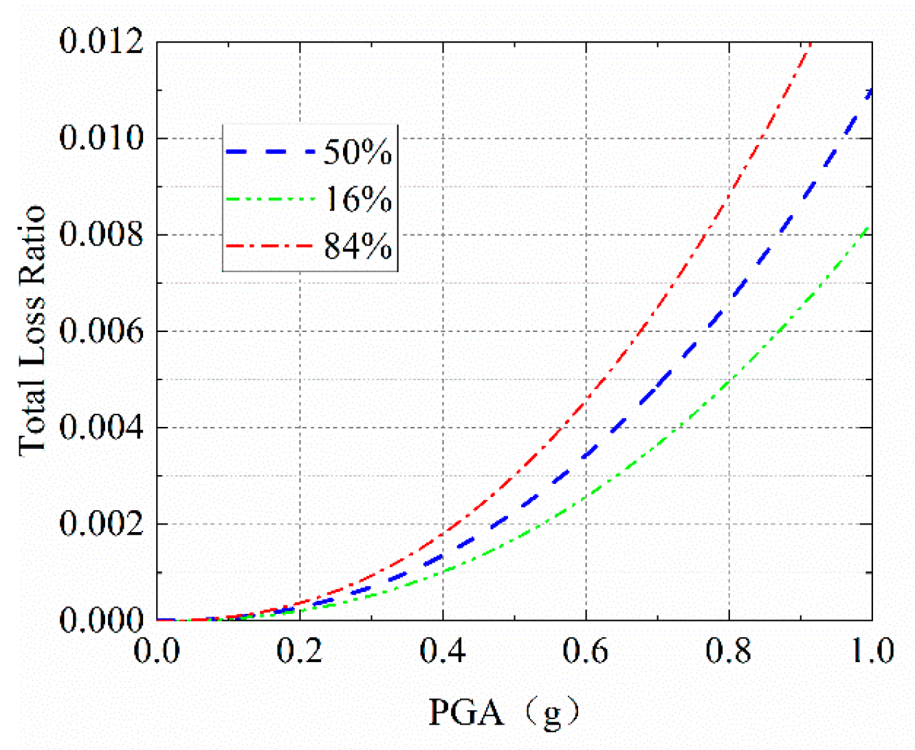
The logarithmic value of the total loss ratio of the models was fitted linearly, as shown in Figure 16, with a Pearson correlation coefficient of 0.9412 and a goodness-of-fit coefficient R2 of 0.8859. According to Equation (9), its log standard deviation is 0.2876, and the total loss ratio estimation result is shown in Figure 17.
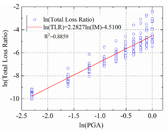
Figure 16.
Fitting curve of the total loss ratio.
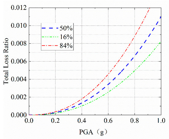
Figure 17.
Prediction curve of the total loss ratio.
4.4. Earthquake Loss of Regional Buildings
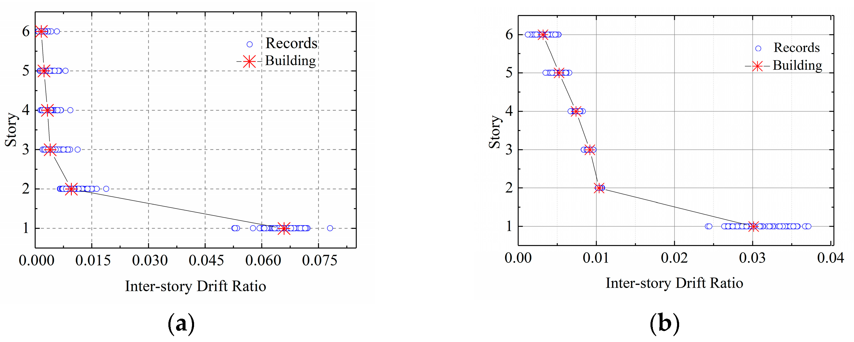
After the SBRS models of all the buildings are established, the predicted values of the loss ratio of each building under different seismic intensities can be obtained using the method described in Section 3.3. Due to the relatively poor seismic performance of RC frame and reinforced masonry structures, most collapsed when the PGA reached 0.5 g, as shown in Figure 18.

Figure 18.
The peak IDR on a typical building: (a) RC frame structure and (b) RM structure.
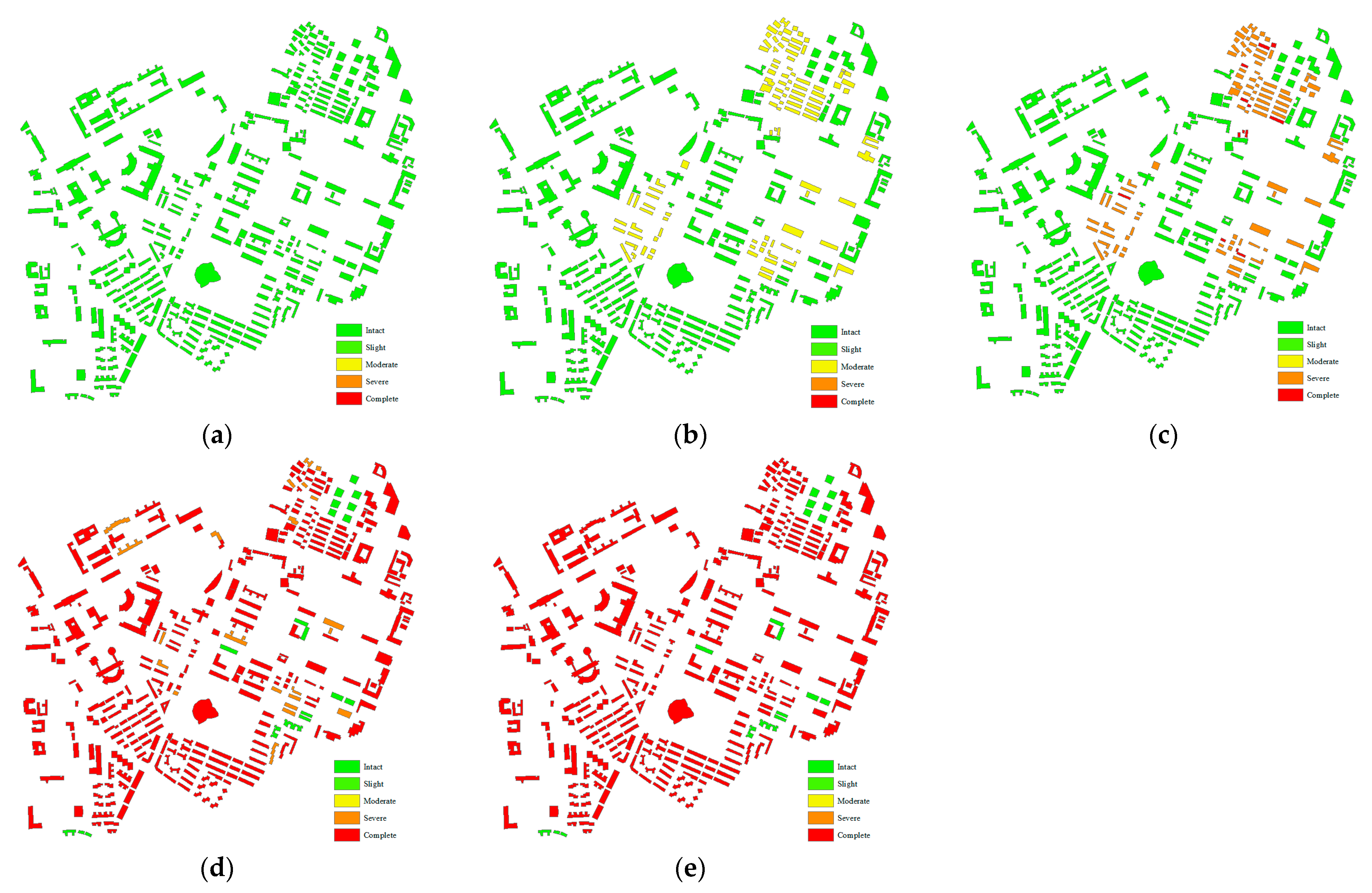
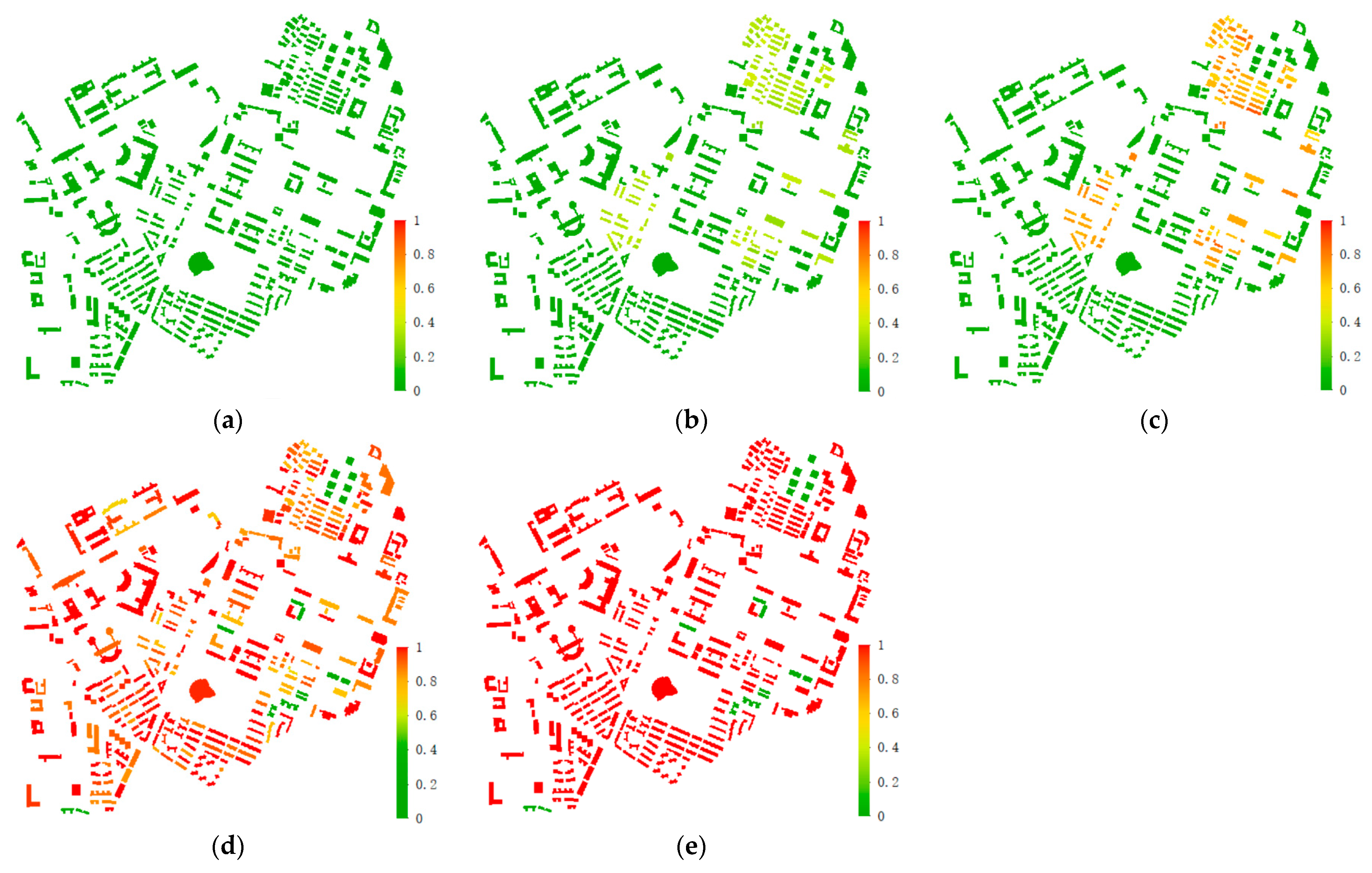
In contrast, the total loss ratio of wall-frame structures in the range of a PGA of 0.5~1.0 g is small and does not change much, so only the PGA ≤ 0.5 g results are shown. The damage state of the building is represented by taking the damage state of the most damaged story. The damage distribution of the buildings at different intensities is shown in Figure 19. The values of the total loss ratio of each building are shown in Figure 20.
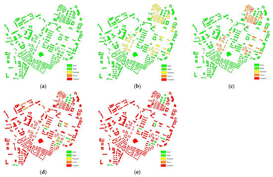
Figure 19.
The damage distribution of the buildings in the study area: (a) PGA = 0.1 g; (b) PGA = 0.2 g; (c) PGA = 0.3 g; (d) PGA = 0.4 g; and (e) PGA = 0.5 g.
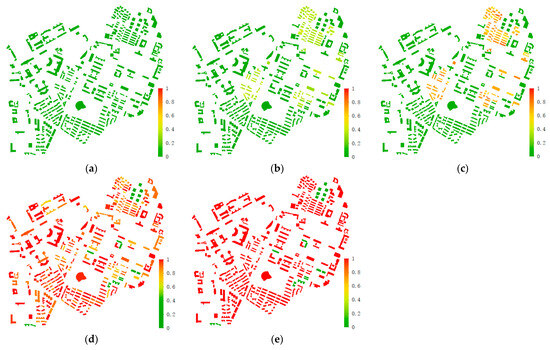
Figure 20.
values of loss ratio for each building in the area: (a) PGA = 0.1 g; (b) PGA = 0.2 g; (c) PGA = 0.3 g; (d) PGA = 0.4 g; and (e) PGA = 0.5 g.
It can be seen that, when PGA ≤ 0.2 g, none of the buildings in the region produced serious damage or collapsed; the loss ratio was at a low level. The generated SBRS models could meet the three-level defense requirements of “no collapse in large earthquakes, repairable in medium earthquakes, and no damage in small earthquakes” required by the specification. As the ground motion intensity continued to increase, the loss ratio of the reinforced masonry structure rose the fastest, and when PGA = 0.3 g, the structure was basically in a more serious damage state or even collapse. When PGA = 0.5 g, the loss ratio of most of the buildings in the region was close to or reached 1, while the buildings showing a dark green color and lower loss ratio were all wall-frame structures. The findings of this study suggest that the impact of earthquakes on buildings varies depending on the level of ground motion intensity and the type of structure. These results are consistent with previous seismic hazard surveys, demonstrating the validity of the SBRS models used in this paper for estimating the earthquake losses in regional buildings.
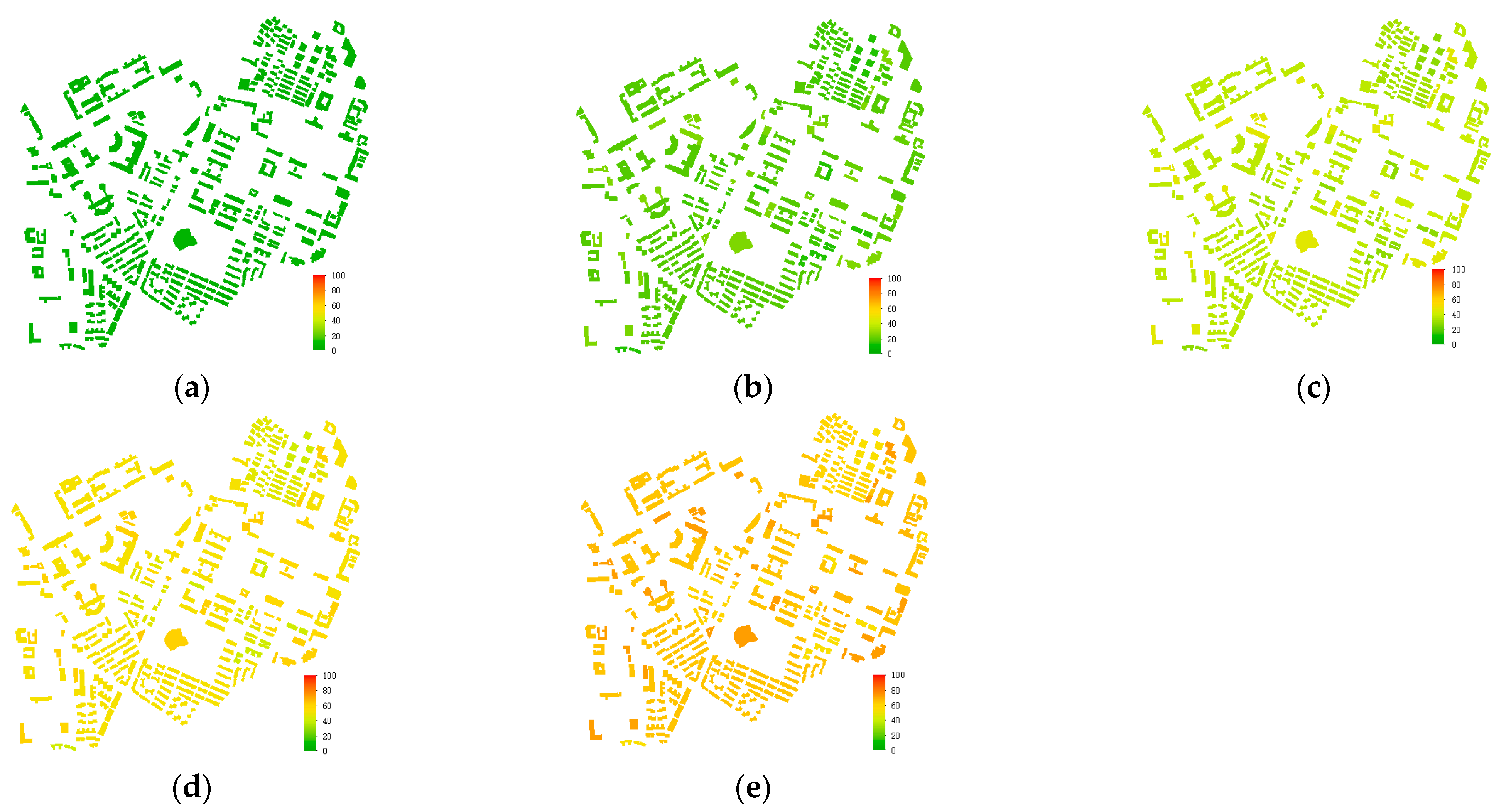
Figure 21 displays the loss ratios based on the HASUZ method. In this study, the RM, RC frame, and RC wall-frame structures are comparable to the HAZUS structural types of RM2, C3, and C2, respectively. According to Lin et al. [46], the seismic design code of the buildings matches the Low-code in HAZUS. The study area includes buildings with various occupancy types, such as RES3af, RES5, COM1, COM4, COM5, COM6, EDU1, and EDU2. The structural repair cost ratio was standardized to facilitate easy comparison with the results presented in this paper.
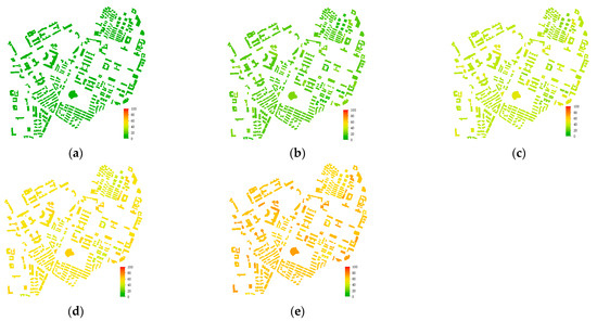
Figure 21.
The loss ratio of each building in the study area uses the HAZUS method: (a) PGA = 0.1 g; (b) PGA = 0.2 g; (c) PGA = 0.3 g; (d) PGA = 0.4 g; and (e) PGA = 0.5 g.
Upon examination, it appears that the disparity in loss ratios for various building types at the same seismic intensity is not readily apparent. Upon comparing Figure 20 and Figure 21, it becomes clear that, while the difference between the two methods is not immediately noticeable at lower seismic intensities, there is a significant difference in loss ratios when the earthquake intensity is high (PGA ≥ 0.4 g). This is due to the fact that this paper’s method is based on the loss ratio ascertained from individual stories, while HAZUS, as a single-degree-of-freedom system, may underestimate the overall seismic loss at higher intensities. In such cases, even if the other stories are relatively undamaged, severe damage to a single story may necessitate the demolition of the entire building.
The corresponding monetization loss values of this paper were obtained by multiplying the corresponding floor areas and the costs per unit area, which assumes values of CNY 0.8, 1.2, and 1.6 thousand for RM, RC frame, and RC wall-frame structures, respectively, as shown in Figure 22.
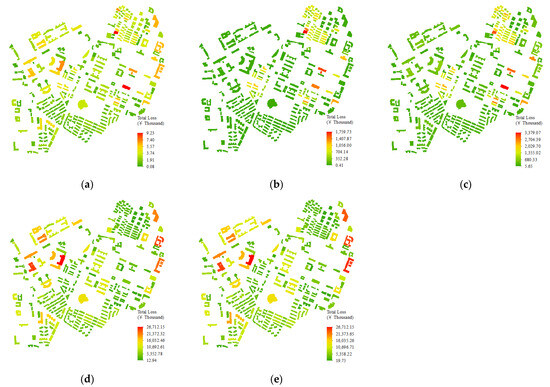
Figure 22.
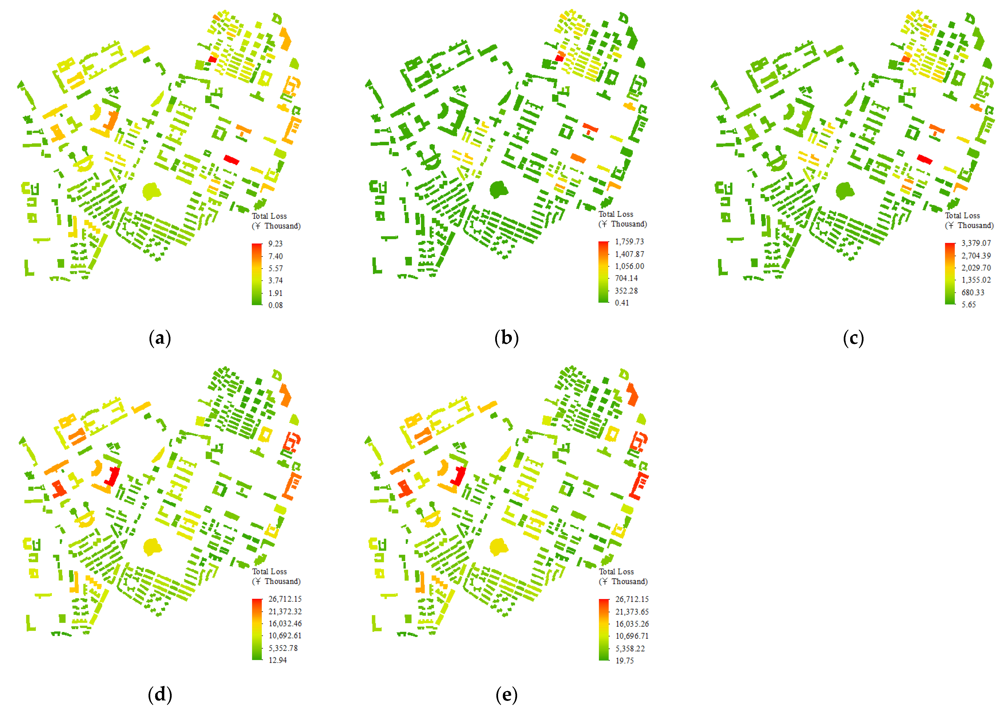
The monetization loss of each building in the study area: (a) PGA = 0.1 g; (b) PGA = 0.2 g; (c) PGA = 0.3 g; (d) PGA = 0.4 g; and (e) PGA = 0.5 g.
We can estimate the total loss for a region by sampling the loss prediction model of a single building. This allows us to statistically determine the probability of exceeding regional loss for different seismic intensities. At the same seismic records, the loss of each building in the region is bound to have a certain correlation, so it can be assumed that the loss ratio of all buildings in the region under different ground motion records obeys the joint lognormal distribution. For each component of , , is the vector of values for an individual building, where is the median value of all the SBRS loss samples at the same seismic record. Based on the loss regression model of each building and the covariance matrix , the joint probability seismic loss model (JPSLM) can be obtained, and its distribution parameters and can be expressed, respectively, as:
The correlation coefficient matrix R of JPSLM can be expressed as:
where is the correlation coefficient of the logarithmic value vector of the loss ratio of the building i and j.
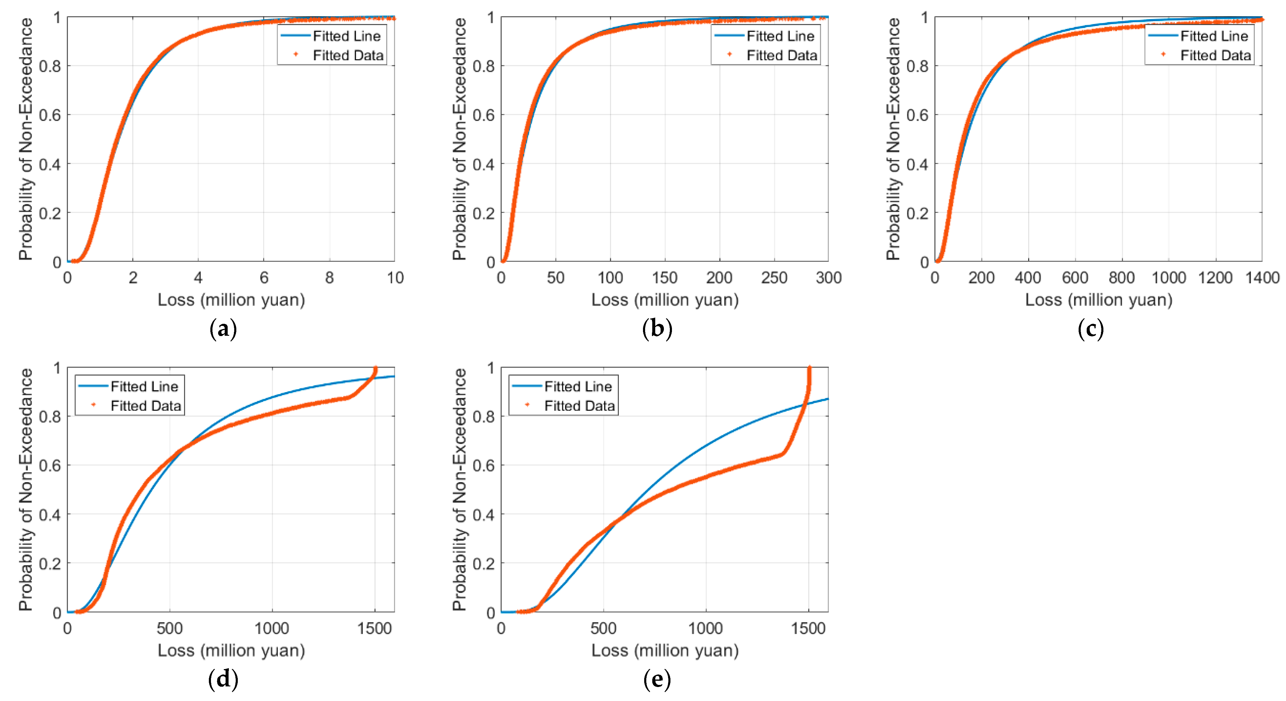
According to Equations (10)–(12), the JPSLM of regional buildings can be obtained. The number of samples taken for each ground shaking intensity is 104, and each building obtains 104 loss ratio samples; the corresponding monetization loss values were obtained by multiplying the corresponding floor areas and costs per unit area, which assumes values of CNY 0.8, 1.2, and 1.6 thousand for masonry, frame, and wall-shear structures, respectively. The loss values obtained from each building for each sampling were aggregated to obtain 104 total regional loss samples, which were fitted assuming that they obeyed a lognormal distribution, and the data points were arranged in ascending order to compare with the fitted curves, as shown in Figure 23.
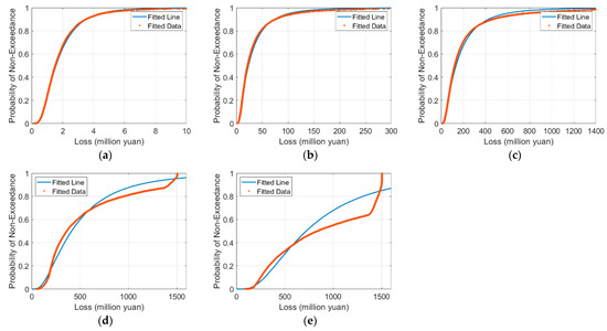
Figure 23.
Non-exceedance probability of total loss of regional buildings: (a) PGA = 0.1 g; (b) PGA = 0.2 g; (c) PGA = 0.3 g; (d) PGA = 0.4 g; and (e) PGA = 0.5 g.
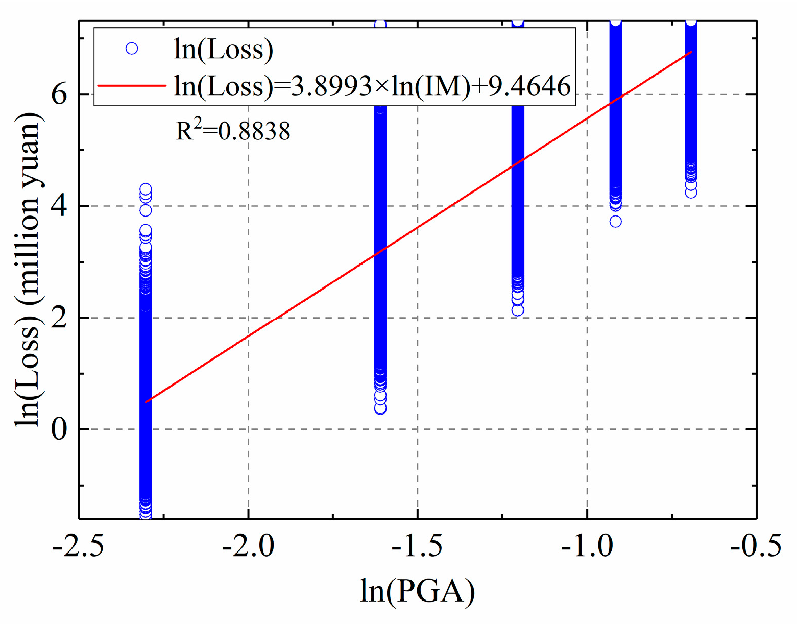
The red data points are the regional loss values from the Monte Carlo sampling in ascending order, which look like a red line because of the density of the data points. In contrast, the blue line is a cumulative distribution curve based on the parameter values of the log-normal distribution fitted to these data points. It can be seen that the two fit well when PGA ≤ 0.3 g, and when PGA ≥ 0.4 g, the data points show a clear trend of rising dash, which is caused by more and more structures in the region collapsing and a steep increase in loss values. As the number of wall-frame structures in the area is small and the damage is minor, they account for a relatively small proportion of the total loss. Thus, the total loss in the area ultimately appears to converge on the cost of rebuilding all the masonry and frame structures, which is approximately CNY 1500 million. Finally, a linear fit to a sample of 104 total regional losses is given in Figure 24, and the predictive model is shown in Figure 25.
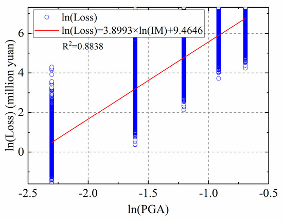
Figure 24.
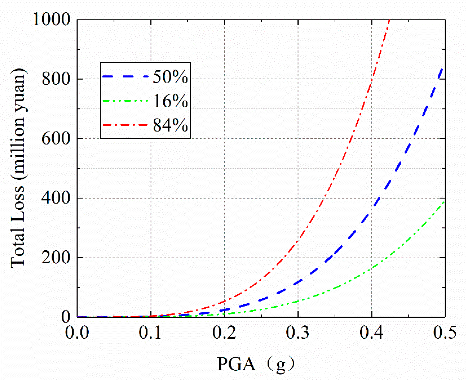
Fitted curve of total loss ratio.
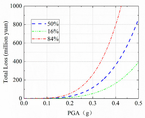
Figure 25.
Prediction curve of total loss ratio.
5. Conclusions
To estimate the earthquake losses of regional buildings, this paper proposes an SBRS modeling method which needs less readily available building information. By combining empirical construction information and the LHS random sampling method, SBRS models can be constructed in an efficient way. The specific conclusions are as follows:
- (1)
- It can establish a structural analysis model with probabilistic accuracy when it is difficult to obtain the specific structural design information of the building, which solves the problem of the rapid and refined modeling of a large number of buildings based on the component level at the urban area scale.
- (2)
- Simulating the structural arrangement and component information of different types of buildings based on the probabilistic approach and combining this with an MDOF centralized mass model makes it possible to use a regional building earthquake loss estimation method based on the seismic capacity of the structure and a dynamic time history analysis, which considers estimation accuracy and computational efficiency.
The layouts of different types of buildings can vary widely depending on region. The SBRS model presented in this paper takes a general approach to consider the impact of design parameters, such as material strength and content size, on the seismic capacity of a structure and earthquake losses. This probabilistic approach helps to improve the accuracy of regional earthquake loss estimation. However, the design forms of modern buildings are complex and varied, and more extensive and in-depth research should be conducted on the modeling process and indexes of the SBRS model according to the design characteristics of different occupancy types. At the same time, having more comprehensive building information will further enhance the accuracy of SBRS modeling and earthquake loss estimation in the future.
Author Contributions
Z.Y. conceived the methodology, conducted the analytical work and wrote the manuscript, Y.L. guided the program code wrote and reviewed the manuscript, and F.X. conceived the concept and guided the research. All authors have read and agreed to the published version of the manuscript.
Funding
This research was funded by the National Natural Science Foundation of China, grant number 52008275.
Institutional Review Board Statement
Not applicable.
Informed Consent Statement
Not applicable.
Data Availability Statement
The raw data supporting the conclusions of this article will be made available by the authors on request.
Acknowledgments
The authors are grateful for the Ground Motion Database of Pacific Earthquake Engineering Research Center.
Conflicts of Interest
The authors declare no conflicts of interest.
References
- Yu, S.Z.; Mu, A.D. Preliminary discussion on the earthquake loss assessment method. Earthq. Eng. Eng. Vib. 2017, 37, 144–151. (In Chinese) [Google Scholar] [CrossRef]
- Zheng, S.S.; Sun, L.F.; Long, L. Urban Earthquake Disaster Loss Assessment: Theoretical Methods, System Development and Application; Science Press: Beijing, China, 2019; pp. 9–13. [Google Scholar]
- Zhou, G.Q.; Mao, Y.; Shi, W.H. Relation between the Earthquake—Affected Population and the Earthquake Losses in Yunnan Area. J. Seismol. Res. 2004, 1, 88–93. (In Chinese) [Google Scholar]
- Chen, Y.; Lin, J.Q.; Liu, J.L.; Cai, Y.J.; Huang, X.K.; Lin, Q.L. Study on rapid assessment method of earthquake direct economic loss. World Earthq. Eng. 2017, 33, 188–193. (In Chinese) [Google Scholar]
- Lu, X.Z.; Cheng, Q.L.; Xu, Z.; Xu, Y.J.; Sun, C.J. Real-time city-scale time-history analysis and its application in resilience-oriented earthquake emergency responses. Appl. Sci. 2019, 9, 3497. [Google Scholar] [CrossRef]
- Federal Emergency Management Agency (FEMA). Multi-Hazard Loss Estimation Methodology—Earthquake Model Technical Manual (HAZUS-MH 2.1); Federal Emergency Management Agency: Washington, DC, USA, 2012.
- Kircher, C.A.; Whitman, R.V.; Holmes, W.T. HAZUS earthquake loss estimation methods. Nat. Hazards Rev. 2006, 7, 45–59. [Google Scholar] [CrossRef]
- Hosseinpour, V.; Saeidi, A.; Nollet, M.J.; Nastev, M. Seismic loss estimation software: A comprehensive review of risk assessment steps, software development and limitations. Eng. Struct. 2021, 232, 111866. [Google Scholar] [CrossRef]
- Yeh, C.H.; Loh, C.H.; Tsai, K.C. Overview of Taiwan earthquake loss estimation system. Nat Hazards 2006, 37, 23–37. [Google Scholar] [CrossRef]
- Chen, H.F.; Sun, B.T.; Chen, X.; Zhong, Y.Z. HAZ-China earthquake disaster loss estimation system. China Civ. Eng. J. 2013, 46 (Suppl. S2), 294–300. (In Chinese) [Google Scholar] [CrossRef]
- Ezz, A.A.E.; Smirnoff, A.; Nastev, M.; Nollet, M.J.; Mcgrath, H. ER2-Earthquake: Interactive web-application for urban seismic risk assessment. Int. J. Disaster Risk Reduct. 2019, 34, 326–336. [Google Scholar] [CrossRef]
- Lu, X.Z.; Han, B.; Hori, M.; Xiong, C.; Xu, Z. A coarse-grained parallel approach for seismic damage simulations of urban areas based on refined models and GPU/CPU cooperative computing. Adv. Eng. Softw. 2014, 70, 90–103. [Google Scholar] [CrossRef]
- Zhang, Y.X.; Zheng, S.S.; Sun, L.F.; Li, L.; Yang, W.; Li, L. Developing GIS-based earthquake loss model: A case study of Baqiao District, China. Bull. Earthq. Eng. 2021, 19, 2045–2079. [Google Scholar] [CrossRef]
- Federal Emergency Management Agency (FEMA). Next-Generation Performance-Based Seismic Design Guidelines Program Plan for New and Existing Buildings; Technical Report 445; Federal Emergency Management Agency: Washington, DC, USA, 2006.
- Yu, X.H. Global Probabilistic Seismic Capacity Analysis of Reinforced Concrete Frame Structures. Master’s Thesis, Harbin Institute of Technology, Harbin, China, 2007. [Google Scholar]
- Lu, D.G.; Liu, Y.; Yu, X.H. Seismic fragility models and forward-backward probabilistic risk analysis in second-generation performance-based earthquake engineering. Eng. Mech. 2019, 36, 12. (In Chinese) [Google Scholar] [CrossRef]
- Federal Emergency Management Agency (FEMA). Seismic Performance Assessment of Buildings: Volume 1—Methodology; Technical Report P58; Federal Emergency Management Agency: Washington, DC, USA, 2012.
- Baradaran Shoraka, M.; Yang, T.Y.; Elwood, K.J. Seismic loss estimation of non-ductile reinforced concrete buildings. Earthq. Eng. Struct. Dyn. 2013, 42, 297–310. [Google Scholar] [CrossRef]
- Shome, N.; Jayaram, N.; Krawinkler, H.; Rahnama, M. Loss estimation of tall buildings designed for the PEER tall building initiative project. Earthq. Spectra 2015, 31, 1309–1336. [Google Scholar] [CrossRef]
- Ramirez, C.; Miranda, E. Building-Specific Loss Estimation Methods and Tools for Simplified Performance-Based Earthquake Engineering; Report 171; the John A; Blume Earthquake Engineering Center, Stanford University: Stanford, CA, USA, 2009. [Google Scholar]
- T/SSC 1-2021; Seismic Destructive Power Evaluation Based on Strong Motion Records. Seismological Society of China Seismological Society of China (SSC): Beijing, China, 2021.
- Zeng, X.; Liu, S.X.; Xu, Z.; Lu, X.Z. Earthquake loss prediction for campus buildings based on FEMA-P58 method: A case study. Eng. Mech. 2016, 33 (Suppl. S1), 113–118. (In Chinese) [Google Scholar] [CrossRef]
- Zeng, X.; Lu, X.Z.; Yang, T.Y.; Xu, Z. Application of the FEMA-P58 methodology for regional earthquake loss prediction. Nat. Hazards 2016, 83, 177–192. [Google Scholar] [CrossRef]
- Xu, Z.; Zhang, H.Z.; Lu, X.Z.; Xu, Y.J.; Zhang, Z.C.; Li, Y. A prediction method of building seismic loss based on BIM and FEMA P-58. Autom. Constr. 2019, 102, 245–257. [Google Scholar] [CrossRef]
- Zhuang, Y.Y.; Xiong, F.; Lu, Y.; Zhang, B.W. Research on modeling method of GIS-based dynamic response analysis model for urban building clusters. World Earthq. Eng. 2021, 7, 137–147. (In Chinese) [Google Scholar] [CrossRef]
- Ruggieri, S.; Liguori, F.S.; Leggieri, V.; Bilotta, A.; Madeo, A.; Casolo, S.; Uva, G. An archetype-based automated procedure to derive global-local seismic fragility of masonry building aggregates: META-FORMA-XL. Int. J. Disaster Risk Reduct. 2023, 95, 103903. [Google Scholar] [CrossRef]
- Spence, R.; So, E.; Ameri, G.; Akinci, A.; Cocco, M.; Cultrera, G.; Franceschina, G.; Pacor, F.; Pessina, V.; Lombardi, A.W.; et al. Earthquake Disaster Scenario Prediction and Loss Modeling for Urban Areas; LESSLOSS, Istituto Universitario di Studi Superiori di Pavia: Pavia, Italy, 2007. [Google Scholar]
- Li, L. Study on Earthquake Damage Prediction of Urban Buildings and Earthquake Economic Losses. Master’s Thesis, Dalian University of Technology, Dalian, China, 2007. [Google Scholar]
- Xiong, C.; Lu, X.Z.; Lin, X.C.; Xu, Z.; Ye, L.P. Parameter determination and damage assessment for THA-based regional seismic damage prediction of multi-story buildings. J. Earthq. Eng. 2016, 21, 461–485. [Google Scholar] [CrossRef]
- Xiong, C.; Lu, X.Z.; Guan, H.; Xu, Z. A nonlinear computational model for regional seismic simulation of tall buildings. Bull. Earthq. Eng. 2016, 14, 1047–1069. [Google Scholar] [CrossRef]
- Steelman, J.S.; Hajjar, J.F. Influence of inelastic seismic response modeling on regional loss estimation. Eng. Struct. 2009, 31, 2976–2987. [Google Scholar] [CrossRef]
- GB 50011-2010; Code for Seismic Design of Buildings. Ministry of Housing and Urban-Rural Development of China (MOHURD): Beijing, China, 2010.
- Huang, J.L. Research on Prediction Method of Seismic Direct Economic Loss of Building Complex. Master’s Thesis, South China University of Technology, Guangzhou, China, 2020. [Google Scholar]
- Su, Q.W.; Liu, Y.H.; Zhao, S.C. Seismic performance of masonry buildings based on wall area. China Civ. Eng. J. 2010, 43 (Suppl. S1), 473–478. (In Chinese) [Google Scholar] [CrossRef]
- GB11968-2020; Standard for Autoclaved Aerated Concrete Blocks. National Standardization Committee (NSC): Beijing, China, 2020.
- GB 50016-2014; Code for Fire Protection Design of Buildings. Ministry of Housing and Urban-Rural Development (MOHURD): Beijing, China, 2014.
- GB 50009-2012; Load Code for the Design of Building Structures. Ministry of Housing and Urban-Rural Development (MOHURD): Beijing, China, 2012.
- Li, G.S. Design Handbook of High-Rise Reinforced Concrete Structure; China Building Industry Press: Beijing, China, 2011; pp. 390–433. [Google Scholar]
- Vamvatsikos, D.; Cornell, C. Incremental dynamic analysis. Earthq. Eng. Struct. Dyn. 2002, 31, 491–514. [Google Scholar] [CrossRef]
- Federal Emergency Management Agency (FEMA). Quantification of Building Seismic Performance Factors; Technical Report 695; Federal Emergency Management Agency: Washington, DC, USA, 2009.
- Structural Engineers Association of California (SEAOC). Performance-Based Seismic Engineering of Buildings: Conceptual Framework, Volume I and II, Vision 2000; Structural Engineers Association of California: Sacramento, CA, USA, 1995. [Google Scholar]
- Grunthal, G. European Macroseismic Scale 1998 (EMS-98); Cahiers du Centre European de Geodynamic et de Seismology 15; Centre European de Geodynamique et de Seismology: Luxembourg, 1998. [Google Scholar]
- GB/T 24335-2009; Classification of Earthquake Damage to Buildings and Special Structures. Ministry of Housing and Urban-Rural Development (MOHURD): Beijing, China, 2009.
- Federal Emergency Management Agency (FEMA). NEHRP Guidelines for the Seismic Rehabilitation of Buildings; Technical Report 273; Federal Emergency Management Agency: Washington, DC, USA, 1997.
- JGJ/T 415-2017; Technical Specification for Post-Earthquake Urgent Assessment and Repair of Buildings. Ministry of Housing and Urban-Rural Development (MOHURD): Beijing, China, 2017.
- Lin, S.B.; Xie, L.L.; Gong, M.S.; Li, M. Performance-based methodology for assessing seismic vulnerability and capacity of buildings. Earthq. Eng. Eng. Vib. 2010, 9, 157–165. (In Chinese) [Google Scholar] [CrossRef]


Disclaimer/Publisher’s Note: The statements, opinions and data contained in all publications are solely those of the individual author(s) and contributor(s) and not of MDPI and/or the editor(s). MDPI and/or the editor(s) disclaim responsibility for any injury to people or property resulting from any ideas, methods, instructions or products referred to in the content. |
© 2024 by the authors. Licensee MDPI, Basel, Switzerland. This article is an open access article distributed under the terms and conditions of the Creative Commons Attribution (CC BY) license (https://creativecommons.org/licenses/by/4.0/).