
Electromagnetic–Thermal Characteristics Analysis of a Tubular Permanent Magnet Linear Generator for Free-Piston Engines

Abstract
:1. Introduction
2. Structures of the FPEG System and TPMLG
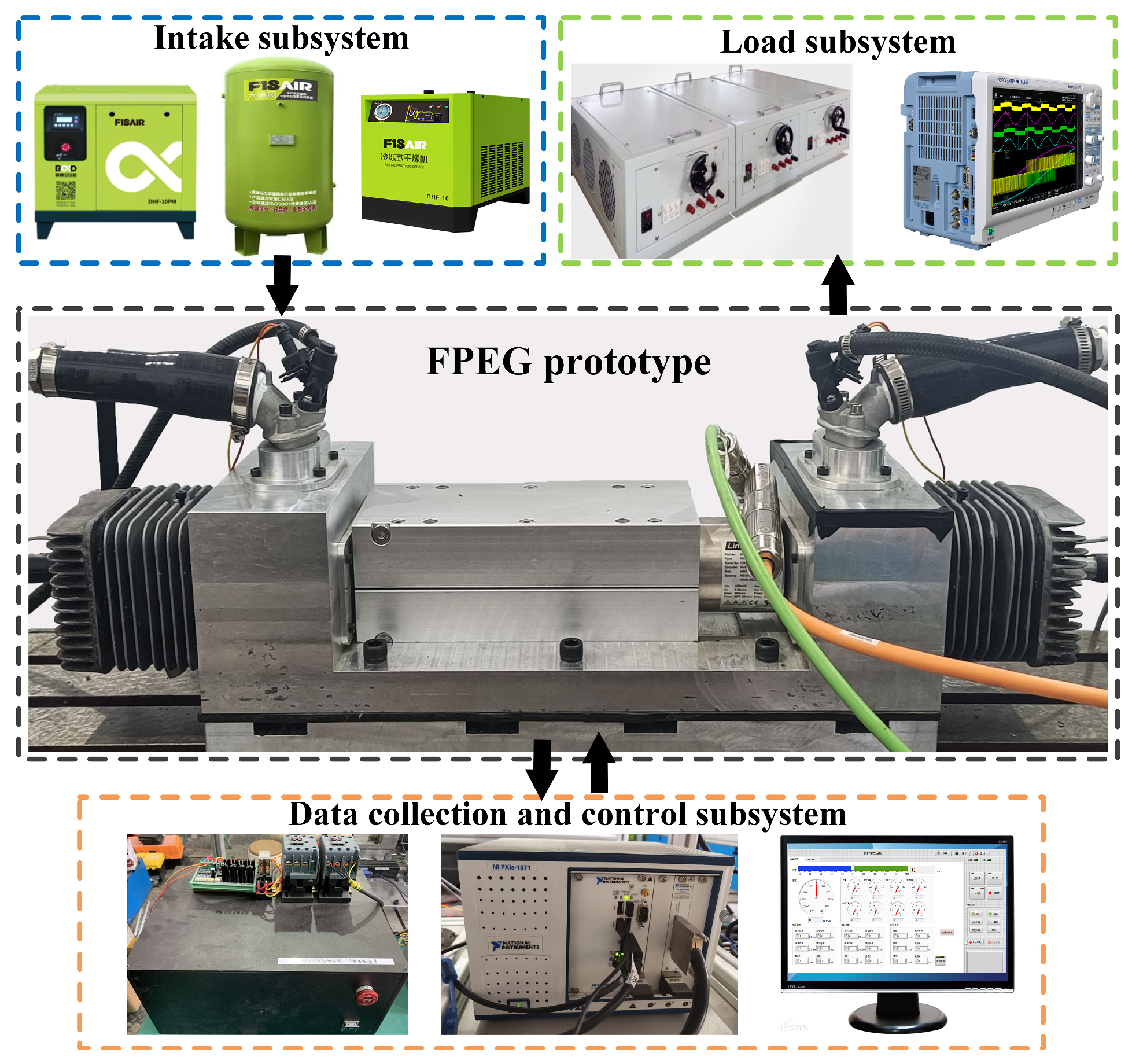
2.1. FPEG System
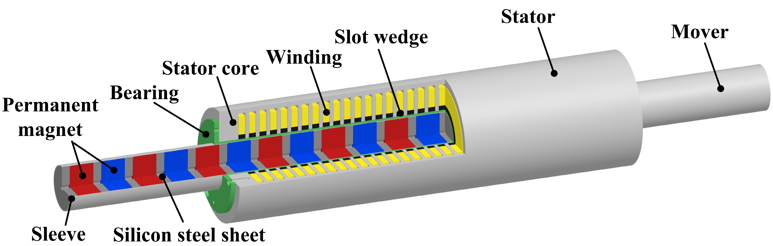
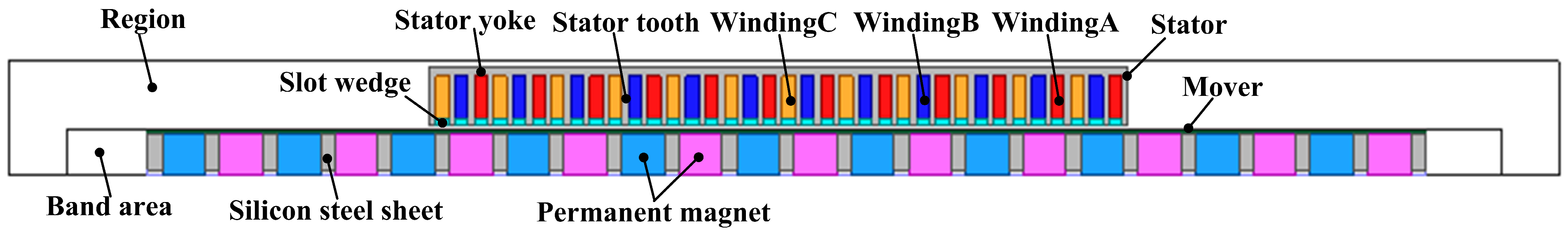
2.2. TPMLG
3. Electromagnetic–Thermal Bidirectional Coupling Model Formulation of TPMLG
3.1. Electromagnetic Finite Element Model of the TPMLG and Loss Calculation
3.2. Thermal–Fluid Finite Volume Model of the TPMLG
- Considering high thermal conductivity and the symmetric structure, it is assumed that the temperatures of the windings and permanent magnets are uniformly distributed in the circumferential direction when the electromagnetic properties of the materials are modified with temperature.
- Some characteristics which are difficult to model are ignored, such as chamfers, fillets, through-holes, and threaded holes.
- Mechanical loss and radiative heat transfer are neglected.
3.2.1. Fundamentals of Thermal–Fluid Analysis
3.2.2. Boundary Conditions
3.2.3. Air Flow
3.2.4. Thermal Conductivity
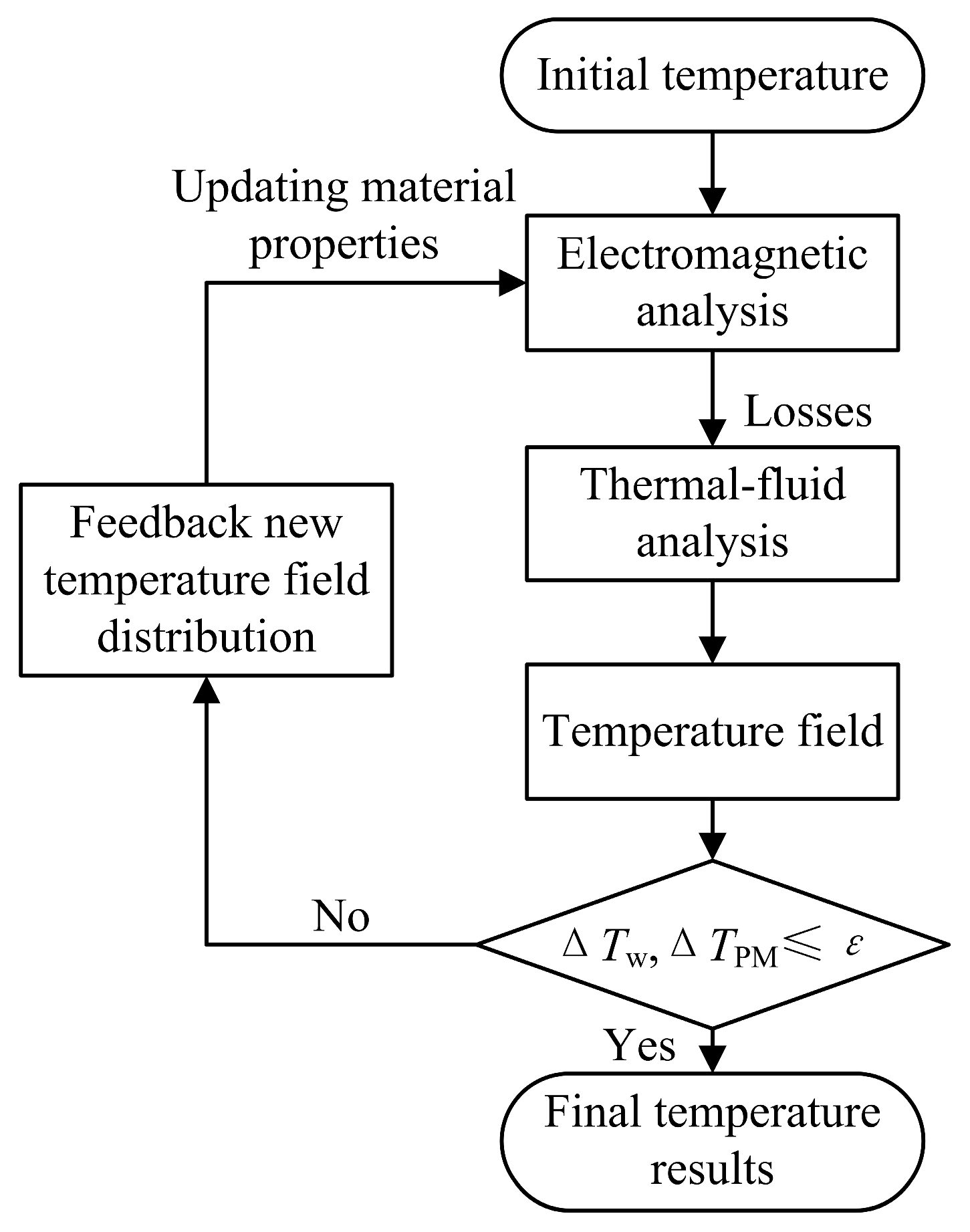
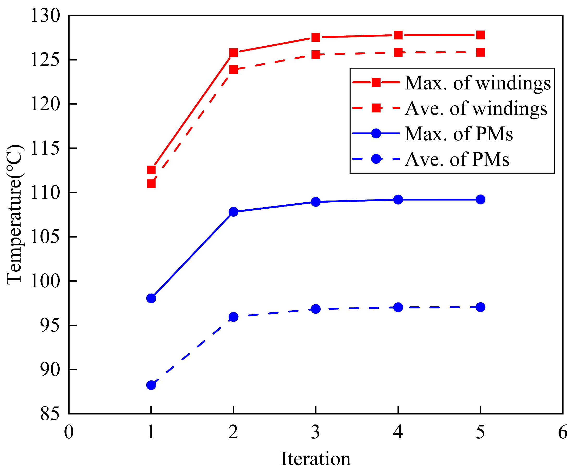
3.3. Electromagnetic–Thermal Bidirectional Coupling Analysis
4. Analysis and Discussions
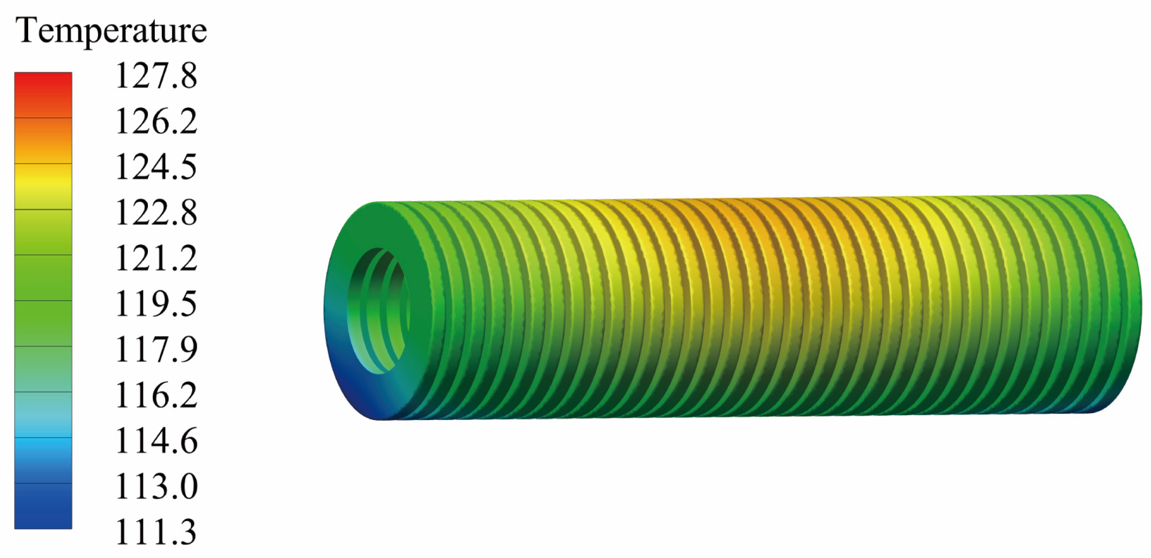
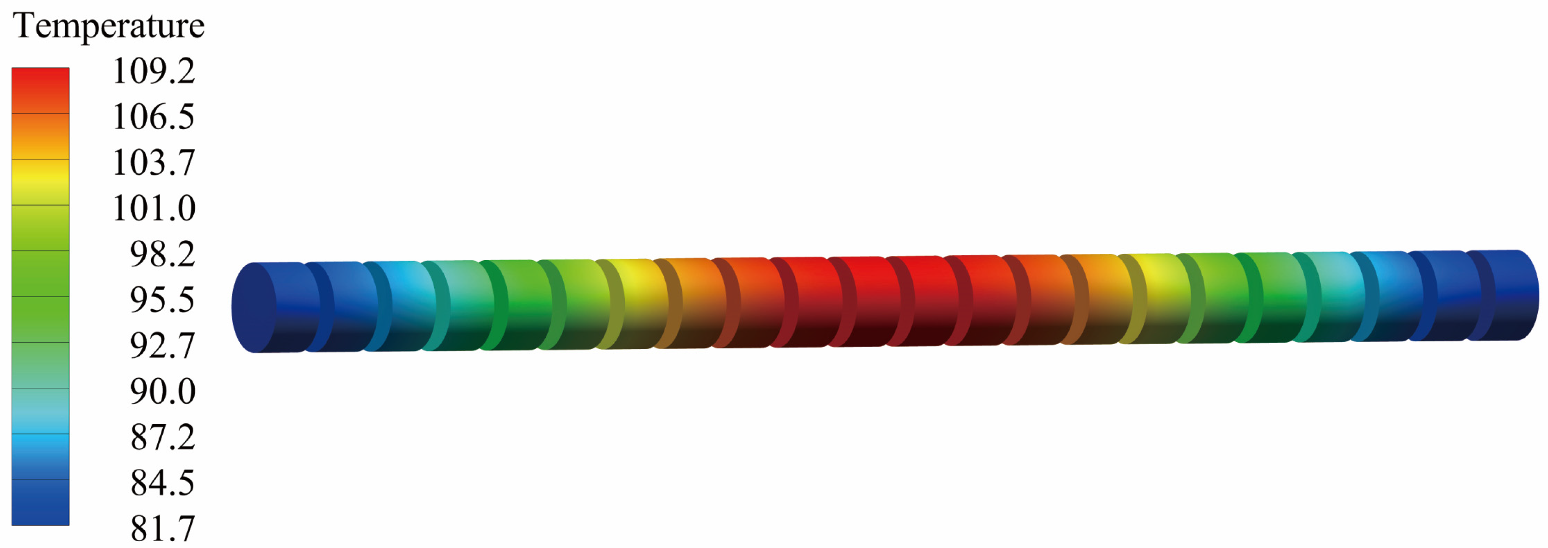
4.1. Temperature Field Distribution of TPMLG
4.2. Influence of Loss on Temperature Rise
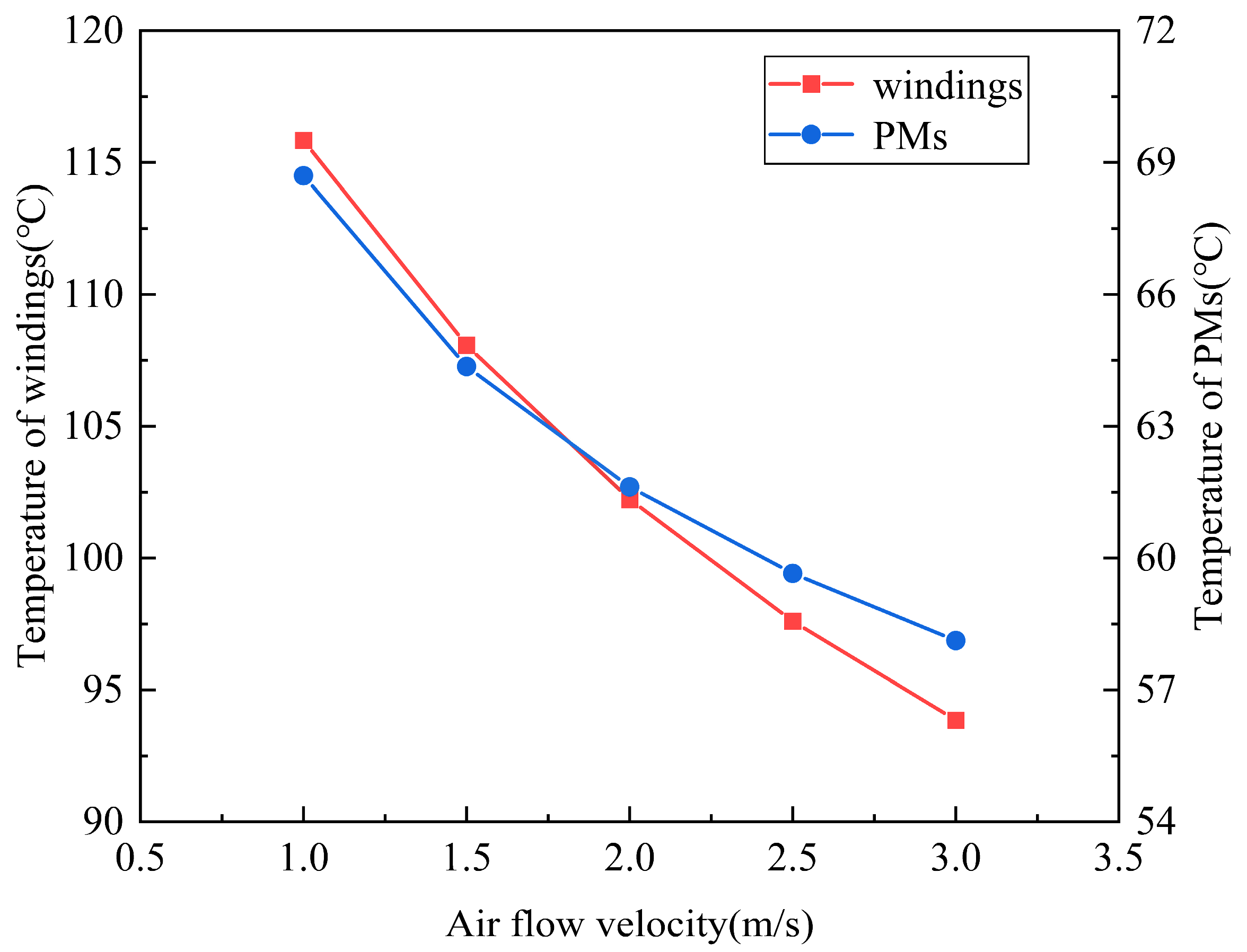
4.3. Influence of Air Flow Velocity on Temperature Rise
5. Conclusions
Author Contributions
Funding
Institutional Review Board Statement
Informed Consent Statement
Data Availability Statement
Conflicts of Interest
References
- Guo, C.; Zuo, Z.; Feng, H.; Roskilly, T. Advances in Free-Piston Internal Combustion Engines: A Comprehensive Review. Appl. Therm. Eng. 2021, 189, 116679. [Google Scholar] [CrossRef]
- Mikalsen, R.; Roskilly, A.P. A Review of Free-Piston Engine History and Applications. Appl. Therm. Eng. 2007, 27, 2339–2352. [Google Scholar] [CrossRef]
- Li, J.; Zuo, Z.; Liu, W.; Jia, B.; Feng, H.; Wang, W.; Smallbone, A.; Roskilly, A.P. Generating Performance of a Tubular Permanent Magnet Linear Generator for Application on Free-Piston Engine Generator Prototype with Wide-Ranging Operating Parameters. Energy 2023, 278, 127851. [Google Scholar] [CrossRef]
- Ahamed, R.; McKee, K.; Howard, I. A Review of the Linear Generator Type of Wave Energy Converters’ Power Take-Off Systems. Sustainability 2022, 14, 9936. [Google Scholar] [CrossRef]
- Trapanese, M.; Boscaino, V.; Cipriani, G.; Curto, D.; Dio, V.D.; Franzitta, V. A Permanent Magnet Linear Generator for the Enhancement of the Reliability of a Wave Energy Conversion System. IEEE Trans. Ind. Electron. 2019, 66, 4934–4944. [Google Scholar] [CrossRef]
- Sun, Y.; Xu, Z.; Zhang, Q.; Liu, L. A Plate Moving-Magnet Linear Generator Designed for Free-Piston Engines. IEEE Access 2020, 8, 75135–75144. [Google Scholar] [CrossRef]
- Hu, Y.; Xu, Z.; Sun, Y.; Liu, L. Electromagnetic Characteristics Analysis of a Tubular Moving Magnet Linear Generator System. Appl. Sci. 2020, 10, 3713. [Google Scholar] [CrossRef]
- Sato, M.; Nirei, M.; Yamanaka, Y.; Bu, Y.; Mizuno, T. High Power Density by Combining of a Double Stator and an Opposite-Magnets Linear Generator in a Dual-Type Free-Piston Engine Generator. Int. J. Appl. Electromagn. Mech. 2021, 65, 355–370. [Google Scholar] [CrossRef]
- Subramanian, J. Design, Modeling and Optimization of Reciprocating Tubular Permanent Magnet Linear Generators for Free Piston Engine Applications. Master’s Thesis, West Virginia University, Morgantown, WV, USA, 2020. [Google Scholar]
- Faiz, J.; Nematsaberi, A. Linear Electrical Generator Topologies for Direct-Drive Marine Wave Energy Conversion—An Overview. IET Renew. Power Gener. 2017, 11, 1163–1176. [Google Scholar] [CrossRef]
- Vese, I.-C.; Marignetti, F.; Radulescu, M.M. Multiphysics Approach to Numerical Modeling of a Permanent-Magnet Tubular Linear Motor. IEEE Trans. Ind. Electron. 2010, 57, 320–326. [Google Scholar] [CrossRef]
- Liu, X.; Yu, H.; Shi, Z.; Guo, R.; Liu, Y. Thermal-Current Density Characteristic Curves for a Single-Side Permanent Magnet Synchronous Linear Motor. Int. J. Appl. Electromagn. Mech. 2019, 61, 477–490. [Google Scholar] [CrossRef]
- Chen, Y.; Yao, Y.; Lu, Q.; Ye, Y.; Huang, X. Electromagnetic and Thermal Coupling Analysis of a Water-Cooled Double-Sided Permanent Magnet Linear Synchronous Motor. In Proceedings of the 2015 18th International Conference on Electrical Machines and Systems (ICEMS), Pattaya, Thailand, 25–28 October 2015; pp. 1136–1140. [Google Scholar]
- Zhu, Z.-Q.; Liang, D. Perspective of Thermal Analysis and Management for Permanent Magnet Machines, with Particular Reference to Hotspot Temperatures. Energies 2022, 15, 8189. [Google Scholar] [CrossRef]
- Boglietti, A.; Cavagnino, A.; Staton, D.; Shanel, M.; Mueller, M.; Mejuto, C. Evolution and Modern Approaches for Thermal Analysis of Electrical Machines. IEEE Trans. Ind. Electron. 2009, 56, 871–882. [Google Scholar] [CrossRef]
- Zhang, S.; Zheng, P.; Yu, B.; Cheng, L.; Wang, M. Thermal Analysis and Experimental Verification of a Staggered-Teeth Transverse-Flux Permanent-Magnet Linear Machine. IET Electr. Power Appl. 2018, 12, 1048–1057. [Google Scholar] [CrossRef]
- Huang, X.; Li, L.; Zhou, B.; Zhang, C.; Zhang, Z. Temperature Calculation for Tubular Linear Motor by the Combination of Thermal Circuit and Temperature Field Method Considering the Linear Motion of Air Gap. IEEE Trans. Ind. Electron. 2014, 61, 3923–3931. [Google Scholar] [CrossRef]
- Xuzhen, H.; Jiaxi, L.; Chengming, Z.; Liyi, L. Calculation and Experimental Study on Temperature Rise of a High OverLoad Tubular Permanent Magnet Linear Motor. IEEE Trans. Plasma Sci. 2013, 41, 1182–1187. [Google Scholar] [CrossRef]
- Gong, J.; Gillon, F.; Brochet, P. Magnetic and Thermal 3D Finite Element Model of a Linear Induction Motor. In Proceedings of the 2010 IEEE Vehicle Power and Propulsion Conference, Lille, France, 1–3 September 2010; pp. 1–6. [Google Scholar]
- Mou, X.J.; Xu, Y.T.; Jiang, F.J. Heat Analysis of a Flat Permanent-Magnet Linear Synchronous Motor. Adv. Mater. Res. 2011, 328, 974–978. [Google Scholar]
- Lu, Q.; Zhang, X.; Chen, Y.; Huang, X.; Ye, Y.; Zhu, Z.Q. Modeling and Investigation of Thermal Characteristics of a Water-Cooled Permanent-Magnet Linear Motor. IEEE Trans. Ind. Appl. 2015, 51, 2086–2096. [Google Scholar] [CrossRef]
- Pei, Z.; Zhao, J.; Song, J.; Zong, K.; He, Z.; Zhou, Y. Temperature Field Calculation and Water-Cooling Structure Design of Coreless Permanent Magnet Synchronous Linear Motor. IEEE Trans. Ind. Electron. 2021, 68, 1065–1076. [Google Scholar] [CrossRef]
- Yu, B.; Zhang, S.; Yan, J.; Cheng, L.; Zheng, P. Thermal Analysis of a Novel Cylindrical Transverse-Flux Permanent-Magnet Linear Machine. Energies 2015, 8, 7874–7896. [Google Scholar] [CrossRef]
- Liu, X.; Yu, H.; Shi, Z.; Xia, T.; Hu, M. Electromagnetic-Fluid-Thermal Field Calculation and Analysis of a Permanent Magnet Linear Motor. Appl. Therm. Eng. 2018, 129, 802–811. [Google Scholar] [CrossRef]
- Pan, D.; Li, L.; Wang, M. Modeling and Optimization of Air-Core Monopole Linear Motor Based on Multiphysical Fields. IEEE Trans. Ind. Electron. 2018, 65, 9814–9824. [Google Scholar] [CrossRef]
- Tong, W.; Sun, R.; Li, S.; Tang, R. Loss and Thermal Analysis for High-Speed Amorphous Metal PMSMs Using 3-D Electromagnetic-Thermal Bi-Directional Coupling. IEEE Trans. Energy Convers. 2021, 36, 2839–2849. [Google Scholar] [CrossRef]
- Zhu, G.; Liu, X.; Li, L.; Chen, H.; Tong, W.; Zhu, J. Cooling System Design of a High-Speed PMSM Based on a Coupled Fluidic–Thermal Model. IEEE Trans. Appl. Supercond. 2019, 29, 1–5. [Google Scholar] [CrossRef]
- Maxwell, A. Maxwell Help; ANSYS Inc.: Canonsburg, PA, USA, 2022. [Google Scholar]
- Li, Y.; Zhang, C.; Xu, X. Bidirectional Electromagnetic–Thermal Coupling Analysis for Permanent Magnet Traction Motors under Complex Operating Conditions. Trans. Can. Soc. Mech. Eng. 2022, 46, 541–560. [Google Scholar] [CrossRef]
- Bertotti, G. General Properties of Power Losses in Soft Ferromagnetic Materials. IEEE Trans. Magn. 1988, 24, 621–630. [Google Scholar] [CrossRef]
- Kim, C.-W.; Kim, J.-M.; Seo, S.-W.; Ahn, J.-H.; Hong, K.; Choi, J.-Y. Core Loss Analysis of Permanent Magnet Linear Synchronous Generator Considering the 3-D Flux Path. IEEE Trans. Magn. 2018, 54, 1–4. [Google Scholar] [CrossRef]
- Yang, S.M.; Zhang, Z.Z. An Experimental Study of Natural Convection Heat Transfer from a Horizontal Cylinder in High Rayleigh Number Laminar and Turbulent Regions. In Institution of Chemical Engineers Symposium Series; Hemisphere Publishing Corporation: London, UK, 1994; Volume 135, p. 185. [Google Scholar]
- Yang, S.M. Improvement of the Basic Correlating Equations and Transition Criteria of Natural Convection Heat Transfer. Heat Transf. Asian Res. 2001, 30, 293–300. [Google Scholar] [CrossRef]
- Bejan, A.; Lage, J.L. The Prandtl Number Effect on the Transition in Natural Convection along a Vertical Surface. J. Heat Transf. 1990, 112, 787–790. [Google Scholar] [CrossRef]


| Parameters | Values | Unit |
|---|---|---|
| Stator tooth width | 2.3 | mm |
| Stator slot width | 4.4 | mm |
| Stator slot number | 36 | - |
| Stator outer diameter | 70 | mm |
| Stator yoke thickness | 3 | mm |
| Stater length | 240 | mm |
| Permanent magnet diameter | 27 | mm |
| Permanent magnet length | 15 | mm |
| Pole pitch | 20 | mm |
| Mover outer diameter | 28 | mm |
| Mover length | 490 | mm |
| Components | Thermal Conductivity W/(m·K) |
|---|---|
| stator core | 42.5/42.5/3.5 |
| PM | 6.4 |
| casing | 13.4 |
| winding | 387.6 |
| sleeve | 202 |
| insulation paper | 0.14 |
| slot wedge | 0.5 |
| air | 0.0272 |
Disclaimer/Publisher’s Note: The statements, opinions and data contained in all publications are solely those of the individual author(s) and contributor(s) and not of MDPI and/or the editor(s). MDPI and/or the editor(s) disclaim responsibility for any injury to people or property resulting from any ideas, methods, instructions or products referred to in the content. |
© 2024 by the authors. Licensee MDPI, Basel, Switzerland. This article is an open access article distributed under the terms and conditions of the Creative Commons Attribution (CC BY) license (https://creativecommons.org/licenses/by/4.0/).
Share and Cite
Liu, W.; Feng, H.; Li, J.; Jia, B. Electromagnetic–Thermal Characteristics Analysis of a Tubular Permanent Magnet Linear Generator for Free-Piston Engines. Appl. Sci. 2024, 14, 1900. https://doi.org/10.3390/app14051900
Liu W, Feng H, Li J, Jia B. Electromagnetic–Thermal Characteristics Analysis of a Tubular Permanent Magnet Linear Generator for Free-Piston Engines. Applied Sciences. 2024; 14(5):1900. https://doi.org/10.3390/app14051900
Chicago/Turabian StyleLiu, Wenzhen, Huihua Feng, Jian Li, and Boru Jia. 2024. "Electromagnetic–Thermal Characteristics Analysis of a Tubular Permanent Magnet Linear Generator for Free-Piston Engines" Applied Sciences 14, no. 5: 1900. https://doi.org/10.3390/app14051900