Analysis of Pressure Distribution on a Single-Family Building Caused by Standard and Heavy Winds Based on a Numerical Approach

Highlights

What are the main findings?

• Model of strong wind flow around sharp edges;
• Analysis of the impact of strong wind on structures.

What is the implication of the main findings?

• Theoretical and numerical analysis;
• Observations and measurements of impacts on existing facilities;
• Comparison of results depending on the solutions used.

Abstract

The aim of this research is to analyze the pressure distribution caused by wind pressure on the structure of a single-family house. The research object is a model reflecting a real structure, which was damaged in 2018 because of heavy winds. The main idea is to create numerical models using various complex structural analysis software and compare the results. The obtained results will be compared with each other to analyze the impact of various factors, hereinafter referred to as boundary conditions, on the pressure values in characteristic places of the facility. The values closest to the normal distribution will be compared to the actual damage to the house structure. The essence of the research will be the identification of phenomena occurring during the action of heavy winds in global conditions (European and American), considering modifications and different ways of creating seemingly similar numerical models and the way they work. Everything will be compared with each other to find the most optimal design method in the given programs and to obtain wind pressure results that are closest to the real ones.

1. Introduction

Wind engineering as a field of science deals with the method of describing strong wind phenomena using various models reflecting real conditions [1,2]. At the same time, it is possible to use these models to calculate the values of various forces that are the response of any structure to their action. The phenomenon is incredibly difficult since each strong wind is slightly different despite external similarities. In recent decades, engineers have proposed and created increasingly new and more accurate ways of describing meteorological phenomena.

One of the subspecies of strong wind is a tornado [3,4]. The simplest model of the phenomenon presents a column of air in the form of a funnel with its narrower edge directed toward Earth’s surface, where it begins to take shape. Thanks to numerous observations and research, the most important parameters of tornadoes are known. These are the speed values most frequently encountered for hopper diameters up to 1.9 m. The first one is the movement of air particles around the column being formed; in this case, it is 135 m/s. The second speed, more often omitted due to its lower value, is the movement of the entire hopper; values in this case are in the range of 3–8 m/s. It is obvious that in extreme conditions, these values may be higher or lower, and the widest documented tornado had a diameter of 75 m. At the same time, there are cases of standing tornadoes with a moving speed of 0 m/s.

Another important issue is the simultaneous occurrence of various types of forces and changes in their vectors because of the hopper moving. Additionally, one should remember the possibility of sudden changes in the value and direction of forces. The last element is the possible different behavior of air particles around the sharp edges of the object, such as corners, dormers, eaves, etc., where small vortices and local flows may be created with parameters different than those on the rest of the object.

Weather phenomena such as heavy winds, especially tornadoes, are among the most complex issues due to the multitude of component displacements and their mutual interactions [5,6,7]. The model describing the movement of air during the passage of an air vortex is multi-faceted. There are three basic directions of particle movement shown in Figure 1: vertical rising, circular movement with a diameter depending on the height, and horizontal displacement of the entire funnel. The mentioned motion possibilities operate simultaneously and interact with each other, so the motion vector of each air particle is individual. In practice, it would be impossible to describe all vectors separately, so simplified models are used.

Another difficulty is the behavior of particles after encountering an obstacle, e.g., a single-family house [9,10,11,12]. Changing direction or creating small vortices near sharp edges are just some of the possibilities that may occur when a tornado encounters an object in its path.

Ultimately, it is important to remember the mutual influence of the initial movement and the disturbances caused by the obstacle. For example, small vortices behind a building are distorted by the constantly moving tornado.

It is obvious that each tornado and each object encountered are rarely repeatable, which is why describing the phenomenon is such a difficult issue. Creating a model manually is impossible, so you should use the possibilities offered by complex software.

The computer technology industry is one of the fastest growing in the world. Every day, the computational capabilities of computers are improved, and programs are developed to describe models that use the latest technology to create.

To describe an example wind model—it was stated above that each case is individual—it is necessary to use an appropriate work tool.

One of the leading programs for fluid flow testing (CFD) is Ansys. It is an extremely efficient and intuitive tool for computational fluid dynamics. It provides opportunities to, for example, maximize the efficiency of the combustion engine or simulate icing in flight. It provides highly accurate results with accurate and trusted solvers.

The issue of modeling wind pressure and the impact of tornadoes on low-rise buildings is the subject of many studies, including one by A. Jaffe, G. Kopp (2021) [13], in which they discussed simulations of internal pressure in a low-rise building and how it changes during a tornado. For this purpose, they used measurements from a tornado simulator and a computational model based on the single discharge equation with the Helmholtz resonator concept. They found that the internal pressure model was able to reasonably simulate the measured internal pressures in tornado winds.

Another work on the topic of wind pressure on low-rise buildings is the example of G. Kopp, Chieh-Hsun Wu (2020) [14]. They compared wind loads during tornadoes and atmospheric boundary layers and tested the hypothesis about the possibility of separating aerodynamic and static pressure. For their research, they used four Cobra probes placed in the corners of the building and developed a quasi-stationary vector model (QS). Based on the research, they found that the QS model ignores local pressure distributions but predicts the order of their changes, and additionally noted that the curvature of the tornado’s wind field increases the amount of suction on the leeward walls.

Another issue is CFD simulation. The issue is described in more detail in the work of F. Rizzo, et al. (2020) [15]. The authors discussed the results of computational fluid dynamics simulations, and one of the goals of the research was to analyze the impact of modeling the laminar to turbulent transition. In their work, they used a flow model using OpenFOAM implementations as well as the FEM method and the 2DOF Scanlan model. The obtained results showed compliance for the $\gamma -\widetilde{R_{\theta ,t}-SA}$, model, and during the tests, they also estimated the critical flutter velocity.

It is obvious that the future of research is artificial intelligence. It allows, for example, the implementation of an artificial neural network model as described in the work of F. Rizzo, L. Caracoglia (2021) [16]. They investigated vertical displacements induced by wind loads on cable mesh roofs with different geometries using FEA and iteratively improved ANN models. The aim of the research was to predict the movement of roofs under the influence of wind. In their work, the researchers proved that the substitute model can reproduce the complex, geometrically nonlinear behavior of the structure.

To sum up, the aim of this work is to analyze the numerical model in relation to the actual state of the existing structure. Various variables will be checked and their impact on the obtained values of forces and stresses.

2. Theoretical Assumptions in the Ansys Fluent Program [17,18,19,20,21,22]

One of the basic devices for empirically studying aerodynamics is a wind tunnel [23]. It is used to analyze the flow of liquid or gas around objects. The test involves generating continuous air movement in a tunnel, most often resembling a cylinder. Models of the tested objects are placed inside the tube. The main use of tunnels is to measure the force acting on the model and to observe the flow. To visualize the flow, colored fluids are often used, or a smoke blower is used.

In terms of construction, tunnels are divided into closed and open-circuit tunnels. Depending on the size of the tunnel, there are many ways to move the air. In the case of smaller ones, turbines powered by electric motors, nozzles, ailerons, or draft dampers are used. For larger tunnels, integrated systems—ducts—driven by turbine engines are used.

When researching, you should remember a few principles of physics:

• The air leaving the fan is set in turbulent motion, so the use of stabilizers is necessary;
• To eliminate the effect of viscosity on the tunnel walls and obtain the most linear flow, smooth walls are used, and the cross-section is often circular;
• If the model is suspended on cables or stands on a platform, their contribution should be taken into account using correction factors;
• When using a scale other than 1:1 to interpret the results, remember to maintain similarity numbers (e.g., Mach number, Froude number, Strouhal number, Reynolds number).

There are many tunnels of various sizes in the world, but their construction and subsequent use are expensive. Models must be created and prepared, and the results must be prepared considering the scaling of the object. Scientists are looking for alternative solutions that provide results close to real ones with less work, time, and money.

An alternative solution is to use modern computer software [24,25,26,27,28]. It is much more accessible and much cheaper to use, which is why it is becoming more and more popular. Creating even complex numerical models is not time-consuming (compared to scale models). Additionally, the programs have built-in calculators and, thanks to a properly applied theoretical knowledge base (laws of physics), they perform most of the calculations themselves.

The method of operation consists of creating a model of the tested object and then closing it in a tunnel of any shape. To use the open tunnel operation scheme, it is enough to designate the inlet and outlet planes and then enter the parameters of the acting wind. After calculations, the model is ready to analyze the results. The software allows you to observe the shape of the flow line, read the values of forces and moments, and analyze pressure distributions.

We currently demand a lot from the software used in calculations. We can start with smooth and fast work, but above all, precision, and reliability of results. To ensure the latter, programs must base the calculations of their solvers on the laws and principles of physics and mathematics. Below are the most important principles on which Ansys bases its calculations.

2.1. Straight-Line Flows

(a)

Principle of conservation of mass;

The mass conservation equation, also known as the continuity equation, can be written as follows:

$$\frac{\mathbf{\partial }\mathit{p}}{\mathbf{\partial }\mathit{t}}+\mathbf{\nabla }\times \left(\mathit{\rho }\overrightarrow{\mathit{v}}\right)={\mathit{S}}_{\mathit{m}}$$

(1)

Equation (1) is the general form of the mass conservation equation and is valid for incompressible and compressible flows. The source is the mass ${\mathit{S}}_{\mathit{m}}$ added to the continuous phase from the dispersed second phase (e.g., due to evaporation of liquid droplets) and any user-defined sources.

For 2D axisymmetric geometries, the continuity equation is given by Equation (2),

$$\frac{\mathbf{\partial }\mathit{p}}{\mathbf{\partial }\mathit{t}}+\frac{\mathbf{\partial }}{\mathbf{\partial }\mathit{x}}\left(\mathit{\rho }{\mathit{v}}_{\mathit{x}}\right)+\frac{\mathbf{\partial }}{\mathbf{\partial }\mathit{r}}\left(\mathit{\rho }{\mathit{v}}_{\mathit{r}}\right)+\frac{\mathbf{\partial }{\mathit{v}}_{\mathit{r}}}{\mathit{r}}={\mathit{S}}_{\mathit{m}}$$

(2)

where $\mathit{x}$ is the axial coordinate, $\mathit{r}$ is the radial coordinate, ${\mathit{v}}_{\mathit{x}}$ is the axial velocity and ${\mathit{v}}_{\mathit{r}}$ is the radial velocity.

(b)

The principle of conservation of momentum;

The conservation of momentum in an inertial (non-accelerating) reference frame is described by Equation (3)

$$\frac{\mathbf{\partial }}{\mathbf{\partial }\mathit{t}}\left(\mathit{\rho }\overrightarrow{\mathit{v}}\right)+\mathbf{\nabla }\ast \left(\mathit{\rho }\overrightarrow{\mathit{v}}\overrightarrow{\mathit{v}}\right)=-\mathbf{\nabla }\mathbf{p}+\mathbf{\nabla }\ast \left(\overline{\overline{\mathit{\tau }}}\right)+\mathit{\rho }\overrightarrow{\mathit{g}}+\overrightarrow{\mathit{F}}$$

(3)

where $\mathit{\rho }$ is the static pressure, $\overline{\overline{\mathit{\tau }}}$ is the stress tensor (described below), and $\mathit{\rho }\overrightarrow{\mathit{g}}$ and $\overrightarrow{\mathit{F}}$ are the gravitational force and external body forces (for example, due to interactions with the dispersed phase), respectively. $\overrightarrow{\mathit{F}}$ also includes other model-dependent source terms, such as porous media and user-defined sources.

The stress tensor $\overline{\overline{\mathit{\tau }}}$ is given by

$$\overline{\overline{\mathit{\tau }}}=\mathit{\mu }\left[\left(\mathbf{\nabla }\overrightarrow{\mathit{v}}+\mathbf{\nabla }{\overrightarrow{\mathit{v}}}^{\mathit{T}}\right)-\frac{\mathbf{2}}{\mathbf{3}}\mathbf{\nabla }\ast \overrightarrow{\mathit{v}}\mathit{I}\right]$$

(4)

where $\mathit{\mu }$ is the molecular viscosity, $\mathit{I}$ is the unit tensor, and the second term on the right is the volume dilation effect.

(c)

User-defined scalar transport equations (UDS);

Ansys Fluent can solve the transport equation for any user-defined scalar (UDS) in the same way that it solves the transport equation for a scalar, such as the mass fraction of a species. In some types of combustion applications or, for example, modeling plasma-enhanced surface reactions, additional scalar transport equations may be needed.

There are two basic subsections for UDS: single-phase and multi-phase flows.

• Single-phase flow

For any scalar ${\mathit{\Phi }}_{\mathit{k}}$, Ansys Fluent solves the equation

$$\frac{\mathbf{\partial }\mathit{p}{\mathit{\Phi }}_{\mathit{k}}}{\mathbf{\partial }\mathit{t}}+\frac{\mathbf{\partial }}{\mathbf{\partial }{\mathit{x}}_{\mathit{i}}}\left(\mathit{\rho }{\mathit{u}}_{\mathit{i}}{\mathit{\Phi }}_{\mathit{k}}-{\mathsf{\Gamma }}_{\mathit{k}}\frac{\mathbf{\partial }{\mathit{\Phi }}_{\mathit{k}}}{\mathbf{\partial }{\mathit{x}}_{\mathit{i}}}\right)={\mathit{S}}_{{\mathit{\Phi }}_{\mathit{k}}}\mathit{k}=\mathbf{1},\dots ,\mathit{N}$$

(5)

where ${\mathsf{\Gamma }}_{\mathit{k}}$ and ${\mathit{S}}_{{\mathit{\Phi }}_{\mathit{k}}}$ are the diffusion coefficient and source term given for each of the $\mathit{N}$ scalar equations. Note that ${\mathsf{\Gamma }}_{\mathit{k}}$ is defined as a tensor in the case of anisotropic diffusivity. The diffusion term is, therefore, $\mathbf{\nabla }\ast \left({\mathsf{\Gamma }}_{\mathit{k}}\ast {\mathit{\Phi }}_{\mathit{k}}\right).$

For isotropic diffusivity, ${\mathsf{\Gamma }}_{\mathit{k}}$ can be written as ${\mathsf{\Gamma }}_{\mathit{k}}\mathit{I}$ where $\mathit{I}$ is the identity matrix.

• Multi-phase flow

For multi-phase flows, Ansys Fluent solves transport equations for two types of scalars: “per phase” and “mixture”. For any scalar $\mathit{k}$ in phase 1, denoted ${\mathit{\Phi }}_{\mathit{l}}^{\mathit{k}}$, Ansys Fluent solves the transport equation within the volume occupied by phase 1.

$$\frac{\mathbf{\partial }{\mathit{\alpha }}_{\mathit{l}}{\mathit{\rho }}_{\mathit{l}}{\mathit{\Phi }}_{\mathit{l}}^{\mathit{k}}}{\mathbf{\partial }\mathit{t}}+\mathbf{\nabla }\ast \left({\mathit{\alpha }}_{\mathit{l}}{\mathit{\rho }}_{\mathit{l}}{{\overrightarrow{\mathit{u}}}_{\mathit{l}}\mathit{\Phi }}_{\mathit{l}}^{\mathit{k}}-{\mathit{\alpha }}_{\mathit{l}}{\mathsf{\Gamma }}_{\mathit{l}}^{\mathit{k}}\mathbf{\nabla }{\mathit{\Phi }}_{\mathit{l}}^{\mathit{k}}\right)={\mathit{S}}_{\mathit{l}}^{\mathit{k}}\mathit{k}=\mathbf{1},\dots ,\mathit{N}$$

(6)

where ${\mathit{\alpha }}_{\mathit{l}}$, ${\mathit{\rho }}_{\mathit{l}}$ and ${\overrightarrow{\mathit{u}}}_{\mathit{l}}$ are the volume fraction, physical density, and velocity of phase 1, respectively. ${\mathsf{\Gamma }}_{\mathit{l}}^{\mathit{k}}$ and ${\mathit{S}}_{\mathit{l}}^{\mathit{k}}$ are the diffusion coefficient and source term, respectively, which need to be determined. In this case, the scalar ${\mathit{\Phi }}_{\mathit{l}}^{\mathit{k}}$ is associated with only one phase (phase 1) and is considered an individual field variable of phase 1.

2.2. Vortex and Rotational Flows

Many important engineering flows involve spinning or rotation, and Ansys Fluent is well-suited to modeling such flows. Swirl flows are common in the combustion process, and swirl is introduced into the burners and combustion chambers to increase residence time and stabilize the flow pattern.

When beginning to analyze swirling or vortex flow, it is important to classify the problem into one of the following five flow categories:

• Axisymmetric flows with swirling or rotation;
• Fully three-dimensional vortex or rotational flows;
• Flows requiring a moving reference frame;
• Flows requiring multiple moving reference frames or mixing planes;
• Flows requiring sliding grids.

(d)

The principle of conservation of momentum for the vortex speed;

The tangential momentum equation for 2D vortex flows can be written as:

$$\frac{\mathbf{\partial }}{\mathbf{\partial }\mathit{t}}\left(\mathit{\rho }\mathit{w}\right)+\frac{\mathbf{1}}{\mathit{r}}\frac{\mathbf{\partial }}{\mathbf{\partial }\mathit{x}}\left(\mathit{r}\mathit{\rho }\mathit{u}\mathit{w}\right)+\frac{\mathbf{1}}{\mathit{r}}\frac{\mathbf{\partial }}{\mathbf{\partial }\mathit{r}}\left(\mathit{r}\mathit{\rho }\mathit{v}\mathit{w}\right)=\frac{\mathbf{1}}{\mathit{r}}\frac{\mathbf{\partial }}{\mathbf{\partial }\mathit{x}}\left[\mathit{r}\mathit{\mu }\frac{\mathbf{\partial }\mathit{w}}{\mathbf{\partial }\mathit{x}}\right]+\frac{\mathbf{1}}{{\mathit{r}}^{\mathbf{2}}}\frac{\mathbf{\partial }}{\mathbf{\partial }\mathit{r}}\left[{\mathit{r}}^{\mathbf{3}}\mathit{\mu }\frac{\mathbf{\partial }}{\mathbf{\partial }\mathit{r}}\left(\frac{\mathit{w}}{\mathit{r}}\right)\right]-\mathit{\rho }\frac{\mathit{v}\mathit{w}}{\mathit{r}}$$

(7)

where $\mathit{x}$ is the axial coordinate, $\mathit{r}$ is the radial coordinate, $\mathit{u}$ is the axial velocity, $\mathit{v}$ is the radial velocity and $\mathit{w}$ is the rotation speed.

(e)

Compressible flows (Mach’s law);

Compressible flows can be characterized by the value of the Mach number:

$$\mathit{M}\equiv \mathit{u}/\mathit{c}$$

(8)

Here $\mathit{c}$ is the speed of sound in the gas $\mathit{c}=\sqrt{\mathit{\gamma }\mathit{R}\mathit{T}}$, while $\mathit{\gamma }$ is the specific heat ratio $\mathit{\gamma }={\mathit{c}}_{\mathit{p}}/{\mathit{c}}_{\mathit{v}}$.

Equation (8) applies to an ideal gas. In the general case of real fluids, the speed of sound is defined in terms of isentropic compressibility as:

$$\mathit{c}=\mathbf{1}/\sqrt{{\left(\frac{\mathbf{\partial }\mathit{\rho }}{\mathbf{\partial }\mathit{p}}\right)}_{\mathit{s}}}$$

(9)

where $\mathit{\rho }$ is the density of the fluid, $\mathit{p}$ is the pressure, and the subscript $\mathit{s}$ means that the partial derivative of the density $\mathit{\rho }$ with respect to the pressure $\mathit{p}$ is taken at constant entropy.

When the Mach number is less than 1.0, the flow is called subsonic. At Mach numbers much less than 1.0 ($\mathit{M}<\mathbf{0.1}$ or thereabouts), compressibility effects are negligible, and changes in gas density with pressure can be safely ignored in flow modeling. As the Mach number approaches 1.0 (which is referred to as the transonic flow regime), compressibility effects become important. When the Mach number exceeds 1.0, the flow is said to be supersonic and may contain shocks and expansion fans that can significantly affect the flow pattern. Ansys Fluent provides a wide range of compressible flow modeling capabilities for subsonic, transonic, and supersonic flows.

(f)

Physics of compressible flows;

Compressible flows are typically characterized by a total pressure ${\mathit{p}}_{\mathbf{0}}$ and a total flow temperature ${\mathit{T}}_{\mathbf{0}}$. In the case of an ideal gas, these quantities can be related to static pressure and temperature in the following way (assuming a constant ${\mathit{C}}_{\mathit{p}}$ parameter):

$$\frac{{\mathit{p}}_{\mathbf{0}}}{\mathit{p}}={\left(\mathbf{1}+\frac{\mathit{y}-\mathbf{1}}{\mathbf{2}}{\mathit{M}}^{\mathbf{2}}\right)}^{\mathit{y}/\left(\mathit{y}-\mathbf{1}\right)}$$

(10)

$$\frac{{\mathit{T}}_{\mathbf{0}}}{\mathit{T}}=\mathbf{1}+\frac{\mathit{y}-\mathbf{1}}{\mathbf{2}}{\mathit{M}}^{\mathbf{2}}$$

(11)

These relationships describe the change in static pressure and temperature in the flow with the change in speed (Mach number) in isentropic conditions. For example, given the ratio of pressures from inlet to outlet (total to static), Equation (10) can be used to estimate the output Mach number that would exist in one-dimensional isentropic flow. For air, Equation (10) predicts choked flow (Mach number of 1.0) with an isentropic pressure ratio of $\mathit{p}/{\mathit{p}}_{\mathbf{0}}=\mathbf{0.5283}$. This choked flow condition will be established at a point in the minimum flow region (for example, at the nozzle throat). In the subsequent expansion of the region, the flow can either accelerate to supersonic flow, where the pressure continues to fall, or return to subsonic flow conditions, slowing down as the pressure increases. If a supersonic flow is exposed to a forced pressure increase, a shock will occur, with a sudden increase in pressure and deceleration across the shock.

(g)

Compressible form of the gas law.

For compressible flows, the ideal gas law is written in the following form:

$$\mathit{\rho }=\frac{{\mathit{p}}_{\mathit{o}\mathit{p}}+\mathit{p}}{\frac{\mathit{R}}{{\mathit{M}}_{\mathit{w}}}\mathit{T}}$$

(12)

where ${\mathit{p}}_{\mathit{o}\mathit{p}}$ is the working pressure, $\mathit{p}$ is the local static pressure relative to the working pressure, $\mathit{R}$ is the universal gas constant and ${\mathit{M}}_{\mathit{w}}$ is the molecular weight. The temperature $\mathit{T}$, will be calculated from the energy equation.

Some compressible flow problems involve fluids that do not behave like ideal gases. For example, flow under very high-pressure conditions usually cannot be accurately modeled under the ideal gas assumption.

3. Numerical Example and Program Comparison

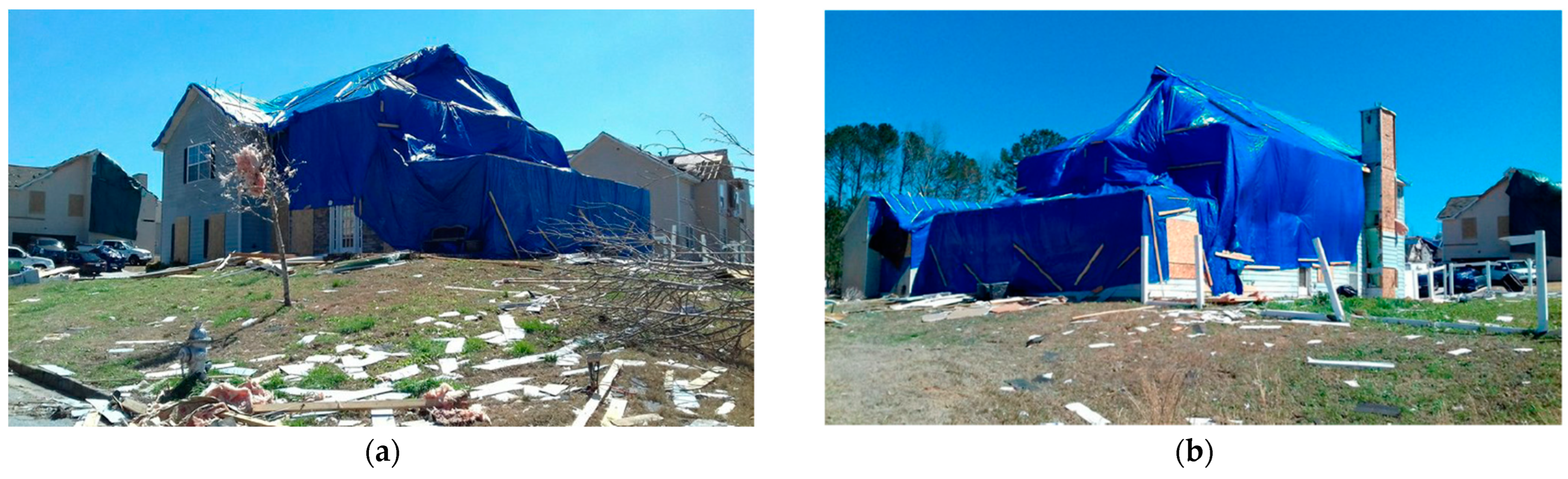
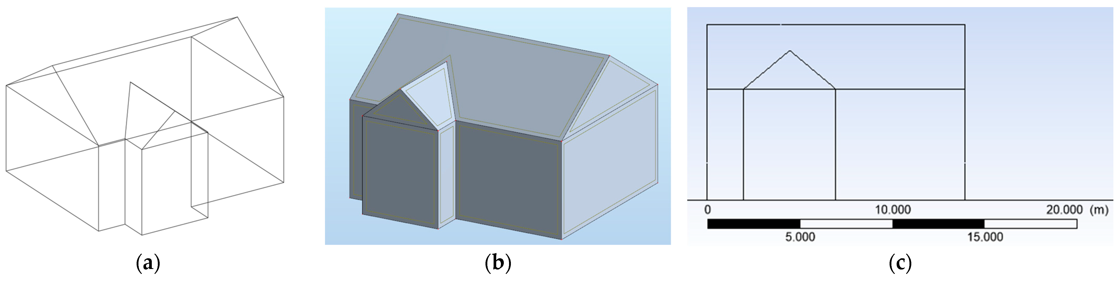
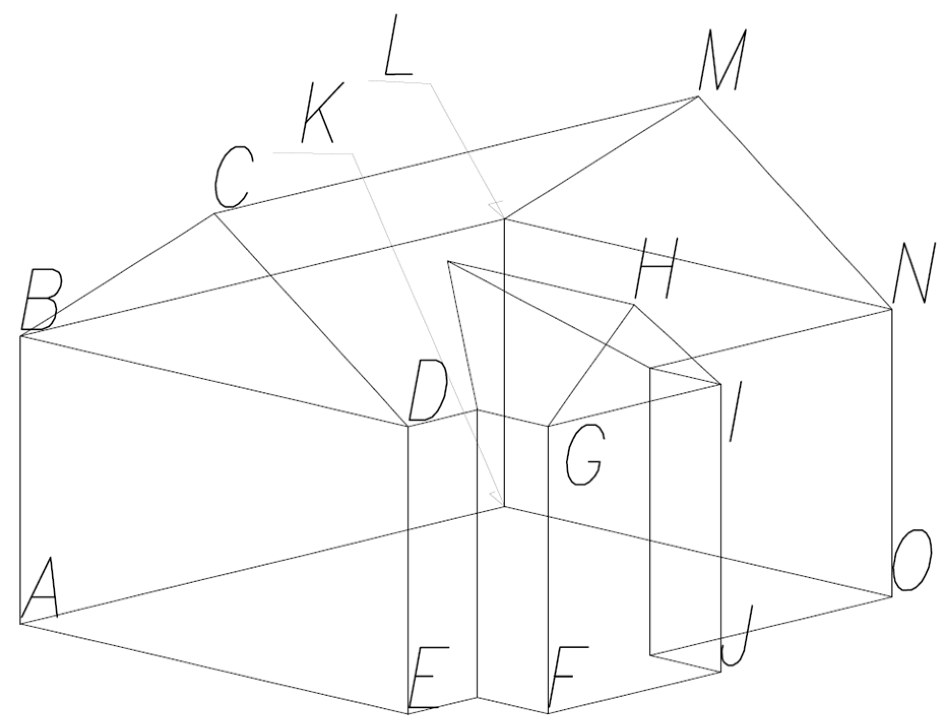
3.1. Description of the Research Subject and the Model Being Created [29,30]

The numerical model created in the article was based on photographic documentation created by the author. The prototype was a single-family building in Fairburn, Georgia, which in 2018 was destroyed by a tornado. Creating the model was described in detail in a separate work by the author [29]. Figure 2 shows a photo of the structure a few days after its destruction. Despite the necessary foil protection, it is visible that the right part of the roof has been torn off, and there are still traces of the tragedy on the ground.

Based on photographic documentation and construction knowledge, a spatial model of the building was created in AutoCAD and then imported into computing programs such as Robot or Ansys. Figure 3 shows the created numerical models.

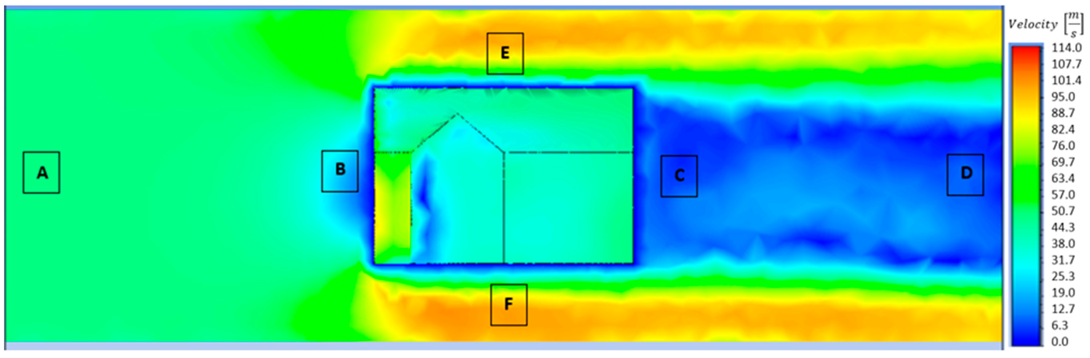
3.2. Scheme of the Conducted Analysis [31,32]

The study involved creating a wind tunnel model, initially in the shape of a horizontal cylinder, in which one of the circular bases was modeled as an air inlet while the opposite one was modeled as an outlet. A model of the analyzed building was placed centrally in the tunnel. The object was oriented with its side wall towards the flow. This is the most likely orientation that could have led to the damage. After setting the wind parameters (initially with a speed of 22 m/s), the flow was simulated.

The analysis covered the stresses arising on the edges of the object and in their vicinity in characteristic places depending on various environmental parameters and at various wind speeds. The object was assumed to be in a wind tunnel with various parameters, with wind flowing from left to right. The general analysis scheme, along with the first assumptions, is presented in Figure 4.

After performing preliminary analyses, the necessary conclusions were drawn, which required the model to be changed, and the fact itself turned out to be so important that it is developed further in the article. In Figure 4, you can see that the pressure graph around the building (in the cross-section these are points E and F) are colored red. This proves the increase in pressure values caused by the interference of the initial waves (inlet wind speed) and the part of the wind reflected from the building walls. It was assumed that the cross-section of the wind tunnel was crucial for the correct analysis of the results; therefore, its parameters (hereinafter referred to as boundary conditions) were checked in detail, and the stress values were compared. To accurately compare the results depending on the boundary conditions, the stress reading locations have been changed, and their number increased. Figure 5 shows characteristic places and corners of the building with descriptions.

3.3. Comparison of Ansys with Robot

The first step necessary for further consideration is to clearly confirm that the selected computer program is reliable and that the results obtained are consistent with the assumptions. For this purpose, an identical building model was prepared in two different programs—Ansys and Robot. The models were loaded with wind at the same speed and then the obtained stress results were compared. The assumed wind speed is 22 m/s and corresponds to the most common wind speed in Poland in accordance with PN-EN 1991-1-4 [33].

The dimensions of the tunnel in Ansys were selected so that the tunnel cross-section was 10 m wider in each direction than the most distant places of the facility, while the length of the tunnel was selected to leave a distance of 20 m in front of and behind the building. The final dimensions were width 33 m, height 29.5 m, length 74 m. It should be noted that the dimensions of the tunnel should not significantly affect the pressure values in the very center of the windward wall because flow disturbances caused by the low capacity of the tunnel primarily affect the air movement around the building, thus affecting the roof and walls parallel to the direction of flow.

Table 1. Comparison of computational programs.

Program:	Stress Values:	Graphic Representation:
Ansys	$\mathbf{332.4}\mathrm{Pa}$
Robot	$\frac{\mathbf{0.29}\mathrm{P}\mathrm{a}+\mathbf{0.36}\mathrm{k}\mathrm{P}\mathrm{a}}{\mathbf{2}}=\mathbf{0.325}\mathrm{k}\mathrm{P}\mathrm{a}=\mathbf{325}\mathrm{P}\mathrm{a}$

presents a comparison of the results obtained in various programs.

Based on the almost identical stresses obtained, regardless of the program, it can be concluded that the results are reliable. The Robot program is a tool used many times by the authors, and its calculations were often compared with those made manually based on applicable standards [33,34,35]. Therefore, it was concluded that the values of pressure on the windward wall can be considered reliable.

4. Dependence of Results on Boundary Conditions

Computer programs have many benefits, but you need to be careful. During modeling, many factors must be considered, which often seem insignificant or not visible graphically at all, which means that no attention is paid to their parameters. The results strictly depend on the entered data and the configuration of boundary conditions, and the user is often unaware of the consequences and importance of seemingly insignificant settings. Listed below are some sample program outputs. The work will present the impact of each of them. These are:

• The shape of the wind tunnel cross-section;
• Internal width;
• Location of the tested object;
• Tunnel length;
• Load duration.

To compare the results, the stress values were read from all corners of the object, obtaining 15 comparison points (Figure 5).

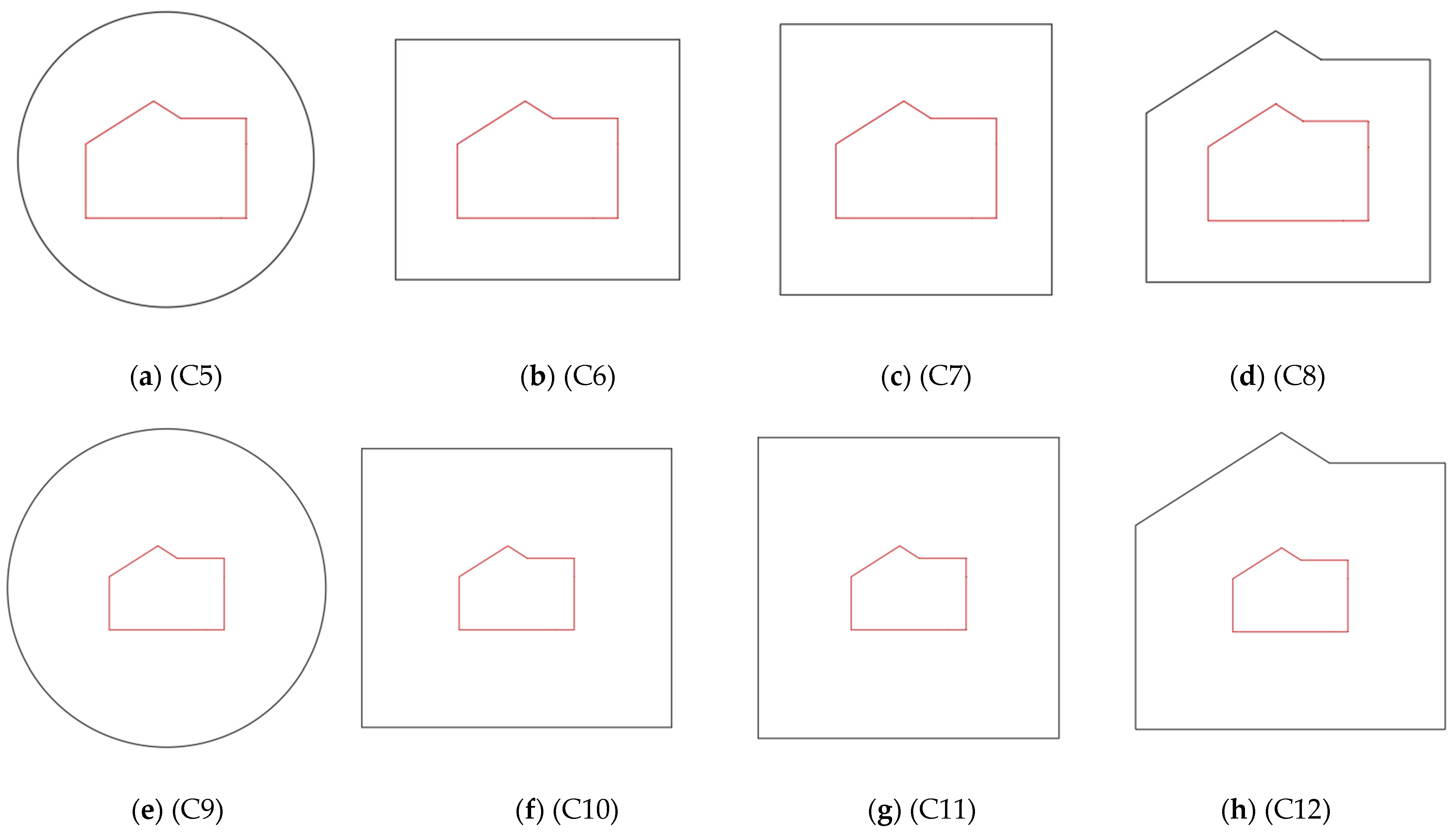
4.1. The Shape of the Wind Tunnel Cross-Section

As mentioned in the section on program comparison, the shape of the cross-section is very important. It influences the behavior of air particles near an object. Additionally, the movement of particles may be disturbed by sharp edges. The shape of the cross-section without sharp edges is a circle or an ellipse. Rectangular and square shapes are also common because of how easy they are to make in real life. The last case considered is the reflection of the shape of the building’s cross-section, less common in the literature, but worth attention. The mentioned shapes are shown in Figure 6. It should be noted that the geometric center of the building cross-section coincides with the geometric center of the figures from the tunnel cross-section. The dimensions of the cross-sections are listed in

Table 2. List of basic parameters for cases C1–C13.

Case	Shape	Width/Diameter [m]	Area [m2]	Free Space around [m2]
C1	Circle	ø18	254.5	149.6
C2	Rectangle	17 × 13.5	229.5	124.6
C3	Square	16 × 16	256	151.1
C4	Building	17 × 13.9	203.5	98.6
C5	Circle	ø24	452.4	347.5
C6	Rectangle	23 × 19.5	448.5	343.6
C7	Square	22	484	379.1
C8	Building	23 × 20.4	409.9	305.0
C9	Circle	ø36	1017.9	913.0
C10	Rectangle	35 × 31.5	1102.5	997.6
C11	Square	34	1156	1051.1
C12	Building	35 × 33.5	1032.9	928.0
C13	Square	50 × 50	2500	2395.1

.

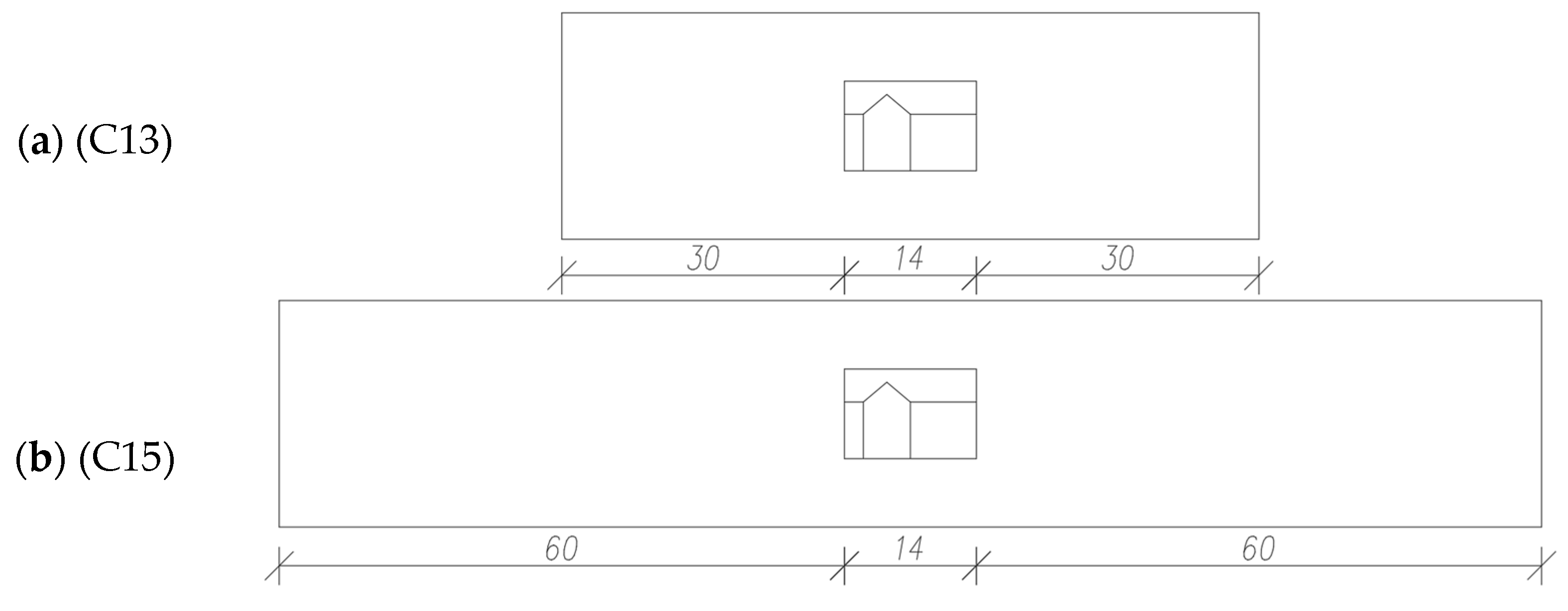
4.2. Internal Width

Another factor is the cross-sectional area, which is directly proportional to the dimensions (depending on the figure: diameter, width, height). As noted in Figure 4, near the building, there are local increases in wind speed caused by low tunnel capacity. To solve this problem, the cross-sections were increased. During the tests, it was noticed that there were still stress concentrations between the building and the tunnel walls, so another increase was applied. Figure 7 shows subsequent cases of previously selected cross-sectional shapes, increasing their dimensions.

Table 2 shows the basic dimensions of each case, C1–C13. Each cross-section shape and dimensions were assigned, respectively: diameter for a circle, width and height for a rectangle and square, and width and height at the highest point for a building. The area formed by the cross-section of the considered object is 104.9 m². The last column of the table corresponds to the difference between the cross-sectional area of each case and the windage area of the building.

To ensure that further increase of the tunnel dimensions does not significantly affect the obtained results, one additional case (C13) was created with an extreme cross-sectional area—almost 10 times larger than the first case.

Based on preliminary observations, case C13 was selected for further analysis and was considered free from the influence of the shape and dimensions of the cross-section; therefore, it was used for further analysis of the influence of other factors.

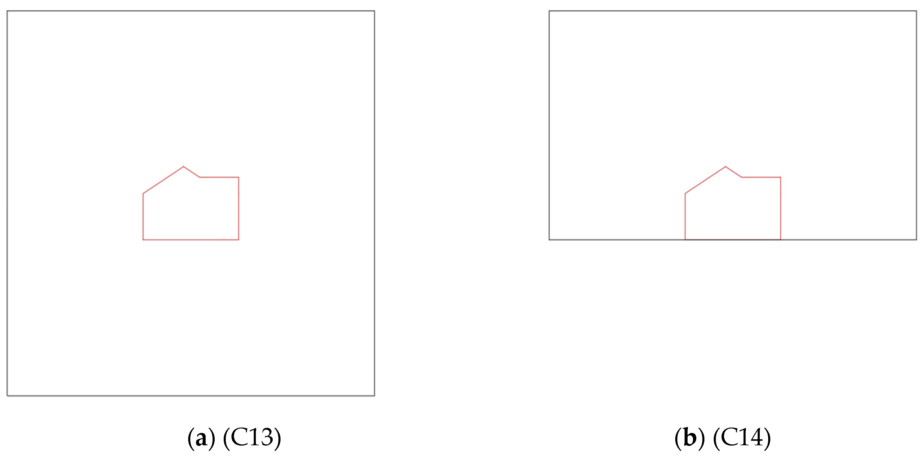
4.3. Setting the Object on the Ground

Numerical tunnels have an advantage over real ones in that the tested object can be located anywhere. In the case of real tunnels, when we want to obtain the case of a flying plane, we can either place it on a platform or suspend it. In both cases, the impact of the solution used on the results should be considered.

To obtain conditions as close as possible to real ones, the object was placed on the ground, reducing square sections of 50 m by 50 m to the 0.00 level, obtaining dimensions of 50 m by 29.75 m.

The article considered two cases: an object in the central part of the cross-section and one located on the ground (Figure 8). Please remember that if placed on the ground, we lose the ability to correctly read the stress values at points at the 0.00 level, i.e., A, E, F, J, G, O. Figure 8 shows a comparison of both cases: an object in the center of the tunnel (C13) and one located on the ground (C14).

4.4. Tunnel Length

Another aspect is the amount of space in front and behind the building, i.e., the length of the tunnel. Initially, 74 m was assumed (30 m distance in front of and behind the building and 14 m length of the facility). The case of increasing this length to 134 m was considered (60 m distance in front of and behind the building and 14 m length of the facility). Figure 9 shows a comparison of the lengths of 74 m and 134 m tunnels.

The newly created cases (C15 and C16) were created because of the extension of the C14 and C15 tunnels. Therefore, they have identical cross-sectional parameters, differing only in their longitudinal dimensions.

4.5. Load Duration

The Ansys program allows you to observe the results in each unit of load duration. The time is introduced through successive load iterations. At the first moment, t = 0, the wind speed inside the tunnel is equal to 0, while the condition of initial speed at the inlet is introduced. As time passes (successive iterations), subsequent wind particles move inside the tunnel up to the exit point.

It is a known fact that the more iterations introduced into the program, the more accurate results can be obtained, but this comes at the expense of greater computing power of the hardware and longer time needed to complete the task. In accordance with the literature assumptions and design knowledge in the Ansys program, the number of iterations is assumed to be 200 as a compromise between the calculation time and the accuracy of the results. However, the question must be asked: How do pressure values change under long-term load?

The article presents a stress analysis for selected cases (C13–C16) under long-term load. The total duration of the load was extended twice, obtaining the number of iterations equal to 400. In this way, another 4 cases C17–C20 were obtained. Figure 10 shows the difference in the isolines symbolizing the wind speed every 100 iterations for the C15 case.

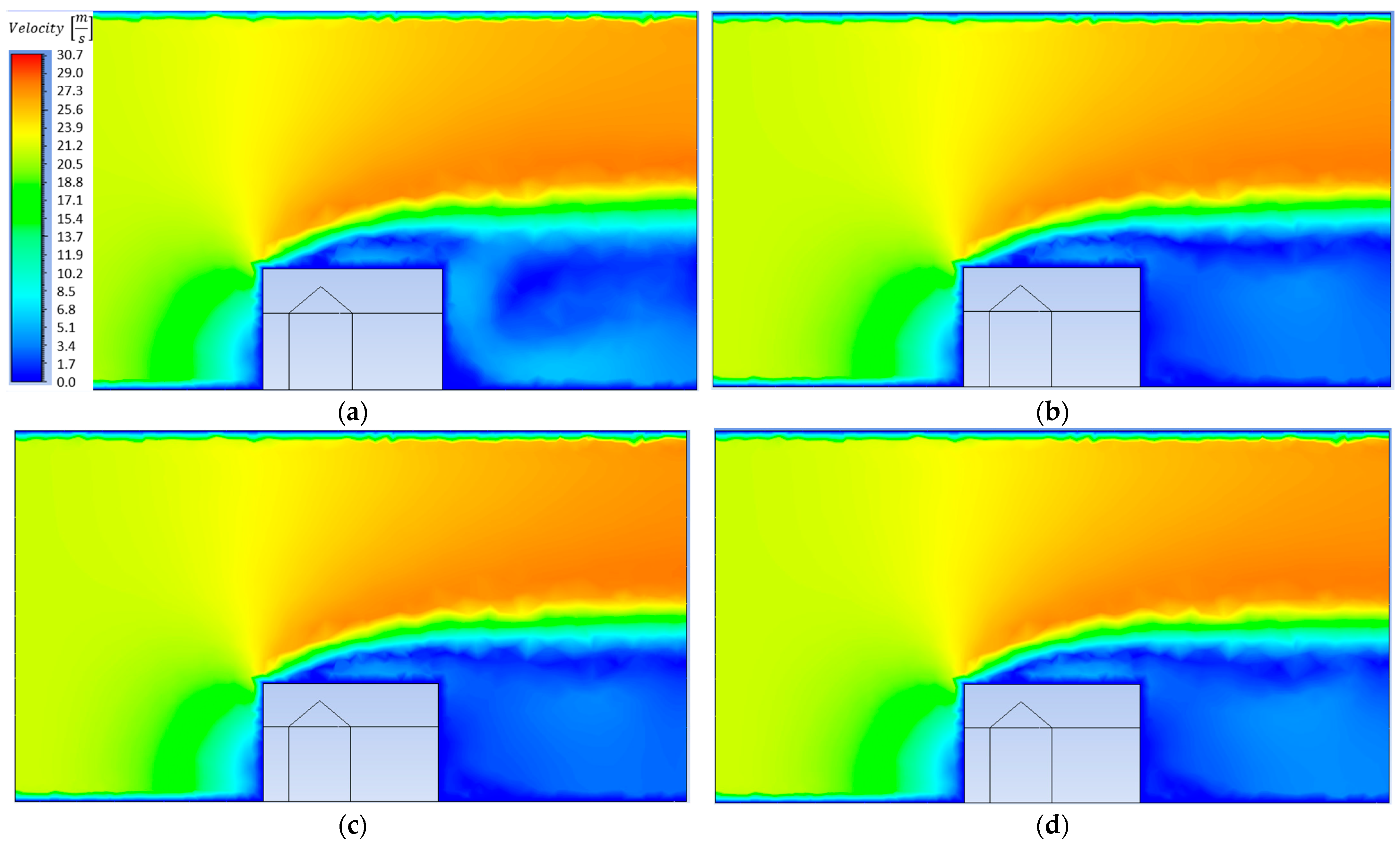
5. Received Results

By introducing various boundary conditions and modifying the calculation parameters in the program, models C1–C20 were created. The analysis of each model consisted of reading the stress values in characteristic places (A–O) and checking the highest and lowest stress values for the entire object.

Table 3. Summary of stresses [MPa] in point A–O for cases C1–C20.

Case\Point	A	B	C	D	E	F	G	H	I	J	K	L	M	N	O
C1	−479.7	−114.1	−193.9	55.2	136.8	−618.8	−44.3	−242.0	−330.9	−290.9	−92.9	−69.1	−101.4	−165.7	−94.2
C2	−353.4	−39.1	−172.5	304.0	104.9	−445.0	−54.6	−221.4	−375.8	−384.9	−50.9	−45.5	−86.5	−198.5	−90.3
C3	−366.2	102.7	−237.4	55.3	96.0	−521.2	−22.2	−172.9	−286.5	−286.3	−66.5	−41.7	−76.1	−180.4	−120.4
C4	−648.3	−90.4	−139.0	386.4	204.9	−587.0	3.9	−543.9	−688.0	−400.5	−109.8	−55.4	−82.3	−180.8	−191.5
C5	−192.4	−48.8	−138.9	−10.7	−91.8	−350.6	−202.6	−155.4	−170.6	−195.5	−43.4	−58.3	−55.4	−77.5	−60.2
C6	−277.9	−195.8	−236.9	−36.4	−108.4	−334.9	−210.3	−144.5	−177.1	−167.7	−43.8	−52.8	−52.4	−91.5	−61.7
C7	−276.5	−128.0	−213.7	−175.1	−135.9	−436.3	−198.0	−207.5	−219.1	−217.8	−96.3	−96.9	−83.1	−119.8	−89.5
C8	−266.0	25.5	−252.6	−60.8	−103.6	−418.5	−155.7	−307.7	−132.1	−154.5	−46.6	−66.3	−38.8	−93.2	−39.2
C9	−151.4	−34.4	−99.9	−89.8	−67.7	−234.2	−92.7	−95.3	−90.7	−94.9	−29.4	−44.9	−80.3	−63.2	−50.0
C10	−96.9	21.8	−112.1	−109.1	−93.2	−256.9	−288.9	−151.4	−159.7	−146.6	−141.6	−138.8	−130.8	−121.8	−118.8
C11	−126.1	25.5	−45.3	−8.7	−52.7	−234.4	−205.5	−93.4	−91.1	−133.1	−43.5	−29.1	−54.0	−83.0	−80.7
C12	−98.7	−20.6	−96.3	−66.6	−66.4	−189.7	−120.4	−161.7	−116.3	−96.0	−45.4	−60.8	−59.9	−89.2	−63.9
C13	−116.4	19.5	−100.1	23.8	−3.5	−148.1	−129.9	−64.2	−52.1	−54.8	−59.5	−72.4	−48.2	−44.4	−75.8
C17	−41.5	94.9	−49.9	47.9	30.5	−94.8	−80.8	−40.0	−33.0	−27.8	−19.8	−18.3	−15.6	−16.5	−20.5
C14	88.1	99.3	−34.1	−16.8	104.8	9.3	−134.5	−36.9	−18.2	−40.2	−19.0	−21.6	−22.3	−21.4	−19.9
C18	87.4	102.3	−41.6	−15.0	111.0	2.6	−127.5	−28.6	−21.9	−19.3	−17.5	−20.1	−18.1	−17.4	−14.6
C15	−49.1	−66.5	−115.9	−110.5	−97.9	−202.7	−272.7	−177.7	−116.2	−111.0	−59.8	−60.1	−67.9	−66.6	−63.9
C19	−53.4	−73.4	−140.7	−112.3	−102.9	−202.5	−269.5	−159.5	−112.3	−112.7	−50.1	−56.6	−55.3	−57.1	−53.1
C16	−54.4	−34.9	−108.9	−81.7	−11.5	−256.0	−276.3	−173.6	−154.7	−112.6	−125.5	−133.2	−131.3	−111.9	−92.9
C20	−48.3	−27.6	−100.1	−75.0	−3.7	−250.8	−268.8	−164.2	−154.7	−114.0	−120.4	−118.8	−118.4	−108.5	−93.8

presents a summary of the results obtained—analysis of stresses in characteristic places. Models in which only load duration was tested (C17–C20) were placed immediately following an identical model with a shorter duration (C13–C16).

For better visibility,

Table 4. List of maximum stresses [MPa] for the entire object for cases C1–C20.

Case\Value	C1	C2	C3	C4	C5	C6	C7	C8	C9	C10
Max	1016.2	1199.5	1035.7	1472.5	573.9	567.3	507.4	608.0	430.4	378.5
Min	−1884.3	−1993.6	−1779.1	−2047.7	−1429.0	−930.7	−928.0	−1306.0	−507.8	−792.2
Case\Value	C11	C12	C13	C17	C14	C18	C15	C19	C16	C20
Max	433.7	438.5	393.9	427.9	296.0	296.0	519.7	523.4	320.9	327.1
Min	−669.7	−519.8	−475.0	−404.8	−536.2	−531.5	−572.1	−595.5	−583.7	−584.5

additionally presents the extreme values (the largest and the smallest) for the entire facility.

In models 16 and 20, the maximum stress, i.e., 320.9 MPa and 327.1 MPa, are most similar to the initial assumptions compared with the Standard and the Robot program.

The data are presented in the form of graphs separately for each point, and extreme values are presented in Figure 11.

6. Strong Wind Analysis in the Best Parameter Configuration

The issue of high wind is vast, and there are many interpretations of this definition. According to the currently applicable Enhanced Fujita scale [36,37,38,39], we can define the wind category depending on the wind speed. Using the same scale, you can also predict the damage that may occur. The author of the scale divides the wind into groups from EF0 to EF5, assigning each a range of speeds that the wind must reach. Depending on the interpretation, cases from EF1 or EF2 can be considered heavy winds. Three speeds were adopted for further analysis:

(a)

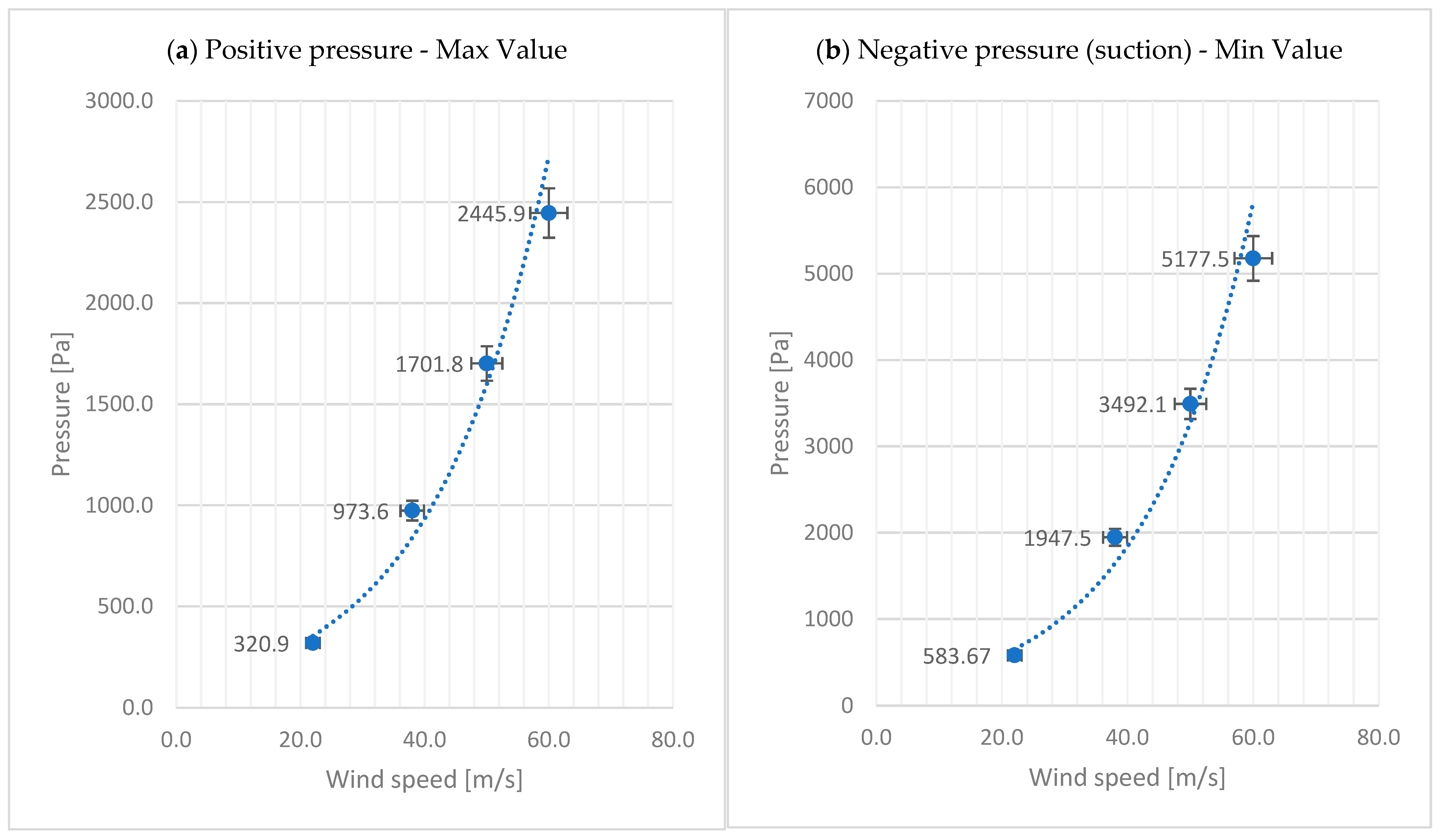
38 m/s (138 km/h) above which the wind can be classified as EF1—case C21;

(b)

50 m/s (178 km/h) above which the wind can be classified as EF2—case C22;

(c)

60 m/s (218 km/h) above which the wind can be classified as EF3—case C23.

Based on the previously obtained values presented in Table 3 and Table 4, case C16 was selected as credible. The model used in the calculations of the three high wind cases is identical to case C16, therefore the stress values from all of them will be compared with it in

Table 5. Stress results depending on wind speed. Comparison of models C21, C22, C23 with the standard case C16.

Case\Point	Velocity [m/s]	A	B	C	D	E	F	G	H
C16	22	−54.4	−34.9	−108.9	−81.7	−11.5	−256.0	−276.3	−173.6
C21	38	−137.9	−49.7	−235.4	−234.8	−52.1	−851.7	−898.4	−577.8
C22	50	−200.5	−46.3	−583.7	−450.1	−96.1	−1516.0	−1536.2	−1073.4
C23	60	−361.5	−280.4	−698.5	−614.9	−155.9	−2245.1	−2258.5	−1603.6
Case\Point	I	J	K	L	M	N	O	Max	Min
C16	−154.7	−112.6	−125.5	−133.2	−131.3	−111.9	−92.9	320.9	−583.7
C21	−504.0	−421.0	−344.8	−392.9	−378.1	−340.1	−334.5	973.6	−1947.5
C22	−908.5	−830.0	−572.7	−575.4	−604.4	−651.6	−704.3	1701.8	−3492.1
C23	−1303.0	−1340.2	−726.7	−767.5	−918.7	−890.8	−932.7	2445.9	−5177.5

.

The extreme values (max—positive and min—negative) characterizing the wind pressure are presented in detail in the graphs in Figure 12.

7. Summary and Conclusions

The article carried out a detailed analysis of the influence of various factors on the obtained pressure values in fifteen characteristic places (A–O) of a residential building, as well as maximum and minimum values. Research was carried out to select the optimal size of the virtual wind tunnel, which, with the lowest possible hardware computing power consumption, allows for obtaining results independent of the influence of boundary conditions. The numerical model reflects the real tunnel (in laboratory conditions) but is also an alternative to it. It allows, with less time and costs, to analyze the impact of wind speed on pressure in various places of the research object. Considerations can also have the opposite effect. Finding the correct (optimal in terms of size) dimensions of wind tunnels may influence the selection of solutions when building real tunnels.

The article created several models that differed from each other in terms of the parameters of the numerical model created in the computational program. Initially, twenty models with constant wind speeds, C1–C20, were created, and then, based on the most optimal one, an additional three with higher speeds, C21–C23. The shape and dimensions of the wind tunnel (C1–C12), the location of the facility (C13–C16), and the influence of the duration of the load (C17–C20) were considered. These are just some of the output parameters that can be edited during the construction of the numerical model.

Based on the results obtained, presented in tables and graphs, we can present the following conclusions:

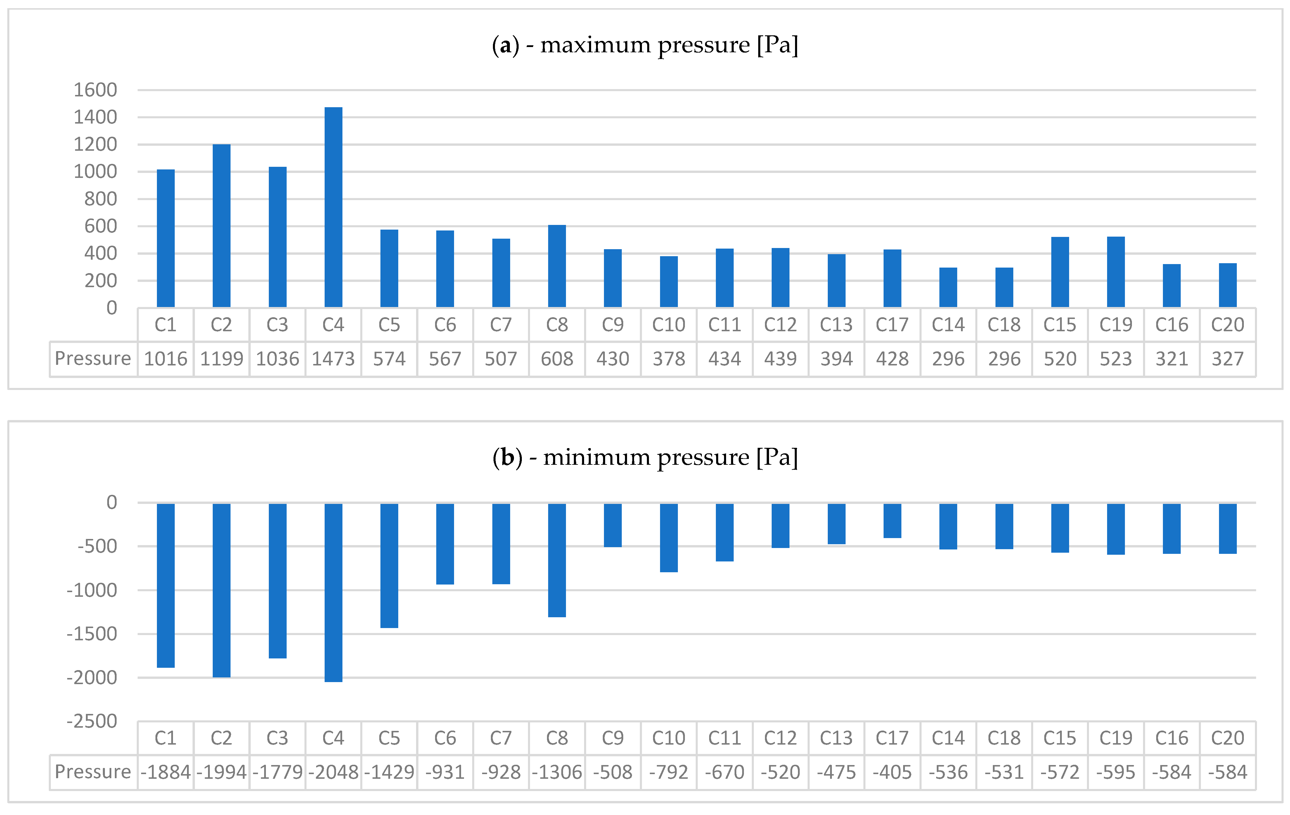
• The results of the obtained pressures, both positive and negative, differ significantly depending on the parameters used: the shape and dimensions (lateral and longitudinal) of the wind tunnel. The initial results were disturbed by the interference of the initial stream and the wave reflected from the building and tunnel walls, which resulted in values of 1473 Pa (C4 model), while the expected value was at the level of 322–325 Pa. Subsequent models created to eliminate the influence of boundary conditions reduced these stresses gradually from 574 Pa (C5 model) to the expected value of 321 Pa (C16 model).
• The location of the tested object (introducing the ground level on which the building is built) (C14 and C16 models) affects not only the pressure values obtained in characteristic places (corners of the object) but also the maximum pressure (pressure on the windward wall). We can analyze the difference in results with one variable (location on the ground) by comparing model C13 versus C14, a decrease from 394 Pa to 296 Pa (24.87%), and C15 versus C16, a decrease from 520 Pa to 321 Pa (38.26%).
• There is a specific (i = 200), easily achievable number of iterations of the computational process (corresponding to the passage of time), after which the impact on the results can be considered negligible. The results can be analyzed by comparing C13 versus C17, an increase from 394 Pa to 428 Pa (8.63%), then C14 versus C18, the value does not change 296 Pa, then C15 versus C19, an increase from 520 Pa to 523 Pa (0.57%), and C16 relative to C20, an increase from 321 Pa to 327 Pa (1.87%).
• It is clearly visible that smaller cross-sections (C1–C4) (average 1181 Pa) significantly overestimate the obtained results due to the concentration of stresses between the model and the tunnel wall. In the next 4 models (C5–C8) (average 564 Pa), the results are normalized, and only in the last part, we obtain reliable results close to the expected value of 320 Pa.
• The shape of the cross-section has a much smaller impact on the values than the size and, above all, the surface corresponding to the free space around the object. The results can be analyzed by comparing models C1–C4 among themselves, then C5–C8 among themselves, and C9–C12 among themselves.
• With a large increase in the cross-section parameters (case C16), it is possible to achieve values independent of the boundary disturbances.
• The analysis of strong wind (presented by trend lines in extreme force diagrams) indicates the non-linearity of the resulting stresses with subsequent increases in output speed.

During the research, other aspects were also noticed, which were also noted in the literature, and are worth considering in continuation of the work. It is, therefore, worth examining the impact of the following factors on the computational model:

• The percentage influence on the obtained results depends on the mesh size of the numerical program;
• Changing the material parameters of the facility and the wind tunnel, such as viscosity, surface type (siding), and roughness.

The presented analysis indicates the need for further research modeling the impact of heavy winds on structures.

References

- Dutkiewicz, M.; Lamparski, T. Ultimate and serviceability limit States of a wooden roof under the wind speed that may cause potential damage to the structure. AIP Conf. Proc. 2023, 2928, 150038. [Google Scholar]
- Dutkiewicz, M.; Hajyalikhani, P.; Lamparski, T.; Whitman, L.; Covarrubias, J. Structural bracing of wooden roofs under the extreme wind. IOP Conf. Ser. Mater. Sci. Eng. 2021, 1203, 022024. [Google Scholar] [CrossRef]
- Dutkiewicz, M. Models of strong wind acting on buildings and infrastructure. IOP Conf. Ser. Mater. Sci. Eng. 2019, 471, 052030. [Google Scholar] [CrossRef]
- Fricker, T.; Friesenhahn, C. Tornado Fatalities in Context: 1995–2018. Weather. Clim. Soc. 2022, 14, 81–93. [Google Scholar] [CrossRef]
- Karstens, C.D.; Samaras, T.M.; Lee, B.D.; Gallus, W.A.; Finley, C.A. Near-ground pressure and wind measurements in tornadoes. Mon. Weather Rev. 2010, 138, 2570–2588. [Google Scholar] [CrossRef]
- Bjerknes, V. The meteorology of the temperate zone and the general atmospheric circulation. Mon. Weather. Rev. 1929, 49, 1–3. [Google Scholar] [CrossRef]
- Alexander, C.R.; Wurman, J.M. Updated mobile radar climatology of supercell tornado structures and dynamics. In Proceedings of the 24th Conference on Severe Local Storms, Savannah, GA, USA, 27–31 October 2008. [Google Scholar]
- A Photo Showing the Movement of a Tornado. Available online: https://nypost.com/wp-content/uploads/sites/2/2018/10/istock-923092852.jpg?quality=75&strip=all (accessed on 20 November 2023).
- Gołębiowska, I.; Dutkiewicz, M.; Lamparski, T.; Hajyalikhani, P. Vibrations of Slender Structures Caused by Vortices. IOP Conf. Ser. Mater. Sci. Eng. 2021, 1203, 022025. [Google Scholar] [CrossRef]
- Haan, F.L., Jr.; Balaramudu, V.K.; Sarkar, P.P. Tornado-induced wind loads on a low-rise building. J. Struct. Eng. 2010, 136, 106–116. [Google Scholar] [CrossRef]
- Horia, H.; Kim, J.D. Swirl ratio effects on tornado vortices in relation to the Fujita scale. Wind. Struct. 2008, 11, 291–302. [Google Scholar]
- Dutta, P.K.; Ghosh, A.K.; Agarwal, B.L. Dynamic response of structures subjected to tornado loads by FEM. J. Wind. Eng. Ind. Aerodyn. 2002, 90, 55–69. [Google Scholar] [CrossRef]
- Jaffe, A.L.; Kopp, G.A. Internal pressure modelling for low-rise buildings in tornadoes. J. Wind. Eng. Ind. Aerodyn. 2021, 209, 104454. [Google Scholar] [CrossRef]
- Kopp, G.A.; Wu, C.-H. A framework to compare wind loads on low-rise buildings in tornadoes and atmospheric boundary layers. J. Wind. Eng. Ind. Aerodyn. 2020, 204, 104269. [Google Scholar] [CrossRef]
- Rizzo, F.; D’Alessandro, V.; Montelpare, S.; Giammichele, L. Computational study of a bluff body aerodynamics: Impact of the laminar-to-turbulent transition modelling. Int. J. Mech. Sci. 2020, 178, 105620. [Google Scholar] [CrossRef]
- Rizzo, F.; Caracoglia, L. Examination of Artificial Neural Networks to predict wind-induced displacements of cable net roofs. Eng. Struct. 2021, 245, 112956. [Google Scholar] [CrossRef]
- Ansys Fluent 12.0 Theory Guide. Available online: https://www.afs.enea.it/project/neptunius/docs/fluent/html/th/main_pre.htm (accessed on 20 November 2023).
- CFD EXPERTS. Ansys Fluent Theory Guide. Available online: https://dl.cfdexperts.net/cfd_resources/Ansys_Documentation/Fluent/Ansys_Fluent_Theory_Guide.pdf (accessed on 20 November 2023).
- Rott, N. On the viscous core of a line vortex. Z. Für Angew. Math. Und Phys. ZAMP 1958, 9, 543–553. [Google Scholar] [CrossRef]
- Sullivan, R.D. A two-cell vortex solution of the navier-stokes equations. J. Aero. Sci. 1959, 26, 767–768. [Google Scholar] [CrossRef]
- Burgers, J.M. A mathematical model illustrating the theory of turbulence. Adv. Appl. Mech. 1948, 1, 171–199. [Google Scholar]
- Rankine, W.J.M. A Manual of Applied Physics, 10th ed.; Charles Griff and Co.: Burbank, IL, USA, 1882; p. 663. [Google Scholar]
- Elementary Knowledge of Real Wind Tunnels. Available online: https://en.wikipedia.org/wiki/Wind_tunnel (accessed on 20 November 2023).
- Takashi, M. Simulation of flying debris using a numerically generated tornado-like vortex. J. Wind. Eng. Ind. Aerodyn. 2011, 99, 249–256. [Google Scholar]
- Lewellen, W.S.; Lewellen, D.C.; Sykes, R.I. Large-eddy simulation of a tornado’s interaction with the surface. J. Atmos. Sci. 1997, 54, 581–605. [Google Scholar] [CrossRef]
- Diwakar, N.; Hangan, H. Numerical study on the effects of surface roughness on tornado-like flows. In Proceedings of the 11th Americas conference on wind engineering (11ACWE), San Juan, Puerto Rico, 22–26 June 2009. [Google Scholar]
- Panneer, S.R.; Millett, P.C. Computer modeling of tornado forces on buildings. Wind. Struct. 2003, 6, 209–220. [Google Scholar]
- Soares Fernandes, Y.M.; Rodrigues Machado, M.; Dutkiewicz, M. The Spectral Approach of Love and Mindlin-Herrmann Theory in the Dynamical Simulations of the Tower-Cable Interactions under the Wind and Rain Loads. Energies 2022, 15, 7725. [Google Scholar] [CrossRef]
- Lamparski, T.; Dutkiewicz, M. The Action of Tornadoes on the Structural Elements of a Wooden Low-Rise Building Roof and Surrounding Objects—Review and Case Study. Appl. Sci. 2023, 13, 4661. [Google Scholar] [CrossRef]
- Lewellen, W.S. Tornado Vortex Theory, the Tornado: Its Structure, Dynamics, Prediction, and Hazards; Geophysical Monograph Series; AGU: Washington, DC, USA, 1993; Volume 79, pp. 19–39. [Google Scholar]
- Alekseenko, S.V.; Kuibin, P.A.; Okulov, V.L. Theory of Concentrated Vortices; Springer: Berlin/Heidelberg, Germany, 2003. [Google Scholar]
- Davies-Jones, R.; Wood, V.T. Simulated Doppler velocity signature of evolving tornado-like vortices. J. Atmos. Ocean. Technol. 2006, 23, 1029–1048. [Google Scholar] [CrossRef]
- EN 1991: Eurocode 1: Actions on Structures Parts 1-1 to 1-7. Available online: https://www.phd.eng.br/wp-content/uploads/2015/12/en.1991.1.1.2002.pdf (accessed on 20 November 2023).
- EN 1990: Eurocode 0: Basis of Structural Design. Available online: https://www.phd.eng.br/wp-content/uploads/2015/12/en.1990.2002.pdf (accessed on 20 November 2023).
- EN 1995: Eurocode 5: Design of Timber Structures. Parts 1-1 to 1-2 and 2. Available online: https://www.phd.eng.br/wp-content/uploads/2015/12/en.1995.1.1.2004.pdf (accessed on 20 November 2023).
- Fujita, T.T. Proposed Characterization of Tornadoes and Hurricanes by Area and Intensity; SMRP Research Paper Number 91; University of Chicago: Chicago, IL, USA, 1970. [Google Scholar]
- Fujita Tornado Damage Scale. Available online: https://www.spc.noaa.gov/faq/tornado/f-scale.html (accessed on 20 November 2023).
- Enhanced Fujita Scale. Available online: https://en.wikipedia.org/wiki/Enhanced_Fujita_scale (accessed on 20 November 2023).
- McDonald, J.R.; Mehta, K.C.; Mani, S. A Recommendation for an Enhanced Fujita Scale (EF-Scale), Revision 2; Wind Science and Engineering, Texas Tech. Univ.: Lubbock, TX, USA, 2006. [Google Scholar]