Fatigue of Bridge Steel Wire: A Corrosion Pit Evolution Model under the Effects of Wind and Vehicles

Abstract

To investigate the damage evolution behavior of corroded steel wires under the influence of alternating loads, a damage evolution model for steel wires based on the theory of continuous damage mechanics was established. The damage evolution process at corrosion pits was simulated by using the element birth and death technique in ANSYS 2020R2. Then, a certain cable-stayed bridge was chosen as the research subject, the stress–time data of the sling were computed using a traffic–bridge–wind simulation analysis model, and the influence of corrosion pit distribution on the mechanical properties and fatigue life of wires under an alternating load was discussed. The results show that, in comparison to single-pitted steel wires, double-pits distributed circumferentially across the cross-section of the steel wires lead to more severe stress concentration, accelerating the damage evolution process and significantly reducing the fatigue life of the steel wires. Conversely, the stress concentration caused by double pits distributed along the longitudinal direction of steel wire is similar to that caused by single pits, and it will be even weaker than that caused by single pits with the change in the relative distance of the double pits. Based on the calculation results of the damage evolution model of steel wire, it was found that the corrosion pit crack nucleation life of steel wire under alternating load accounts for nearly 80% of the fatigue life of steel wire, and different corrosion pit distribution modes will significantly affect the fatigue life of steel wire.

1. Introduction

Due to the complex geographical locations and climatic conditions of cable-stayed bridges, these structures are likely to be continuously affected by the corrosive environment of the surrounding area throughout their construction and operational phases [1]. Furthermore, owing to the lightweight nature and low rigidity of the cable materials used in these structures, they exhibit heightened sensitivity to wind loads, often leading to pronounced vibrations when subjected to wind excitations. Consequently, the cable systems within suspension bridges frequently contend with the synergistic impact of alternating loads and environmental corrosion, potentially culminating in corrosion fatigue damage, thereby precipitating economic losses and safety hazards [2]. Therefore, it is necessary to study the mechanism of corrosion fatigue-damage evolution in suspension bridge cables.

The presence of corrosion pits in high-strength steel wires gives rise to stress concentration, resulting in the formation of high-stress regions at the pit, thereby posing a substantial threat to the structural fatigue life [3]. Addressing the inherent vulnerability of high-strength steel wires to corrosion, various scholars have conducted comprehensive investigations into the intricacies of the fatigue performance of corroded wires. Wang et al. [4] conducted meticulous fatigue-crack propagation-rate tests on high-strength steel wires under diverse stress ratios, concurrently developing a sophisticated numerical model for fatigue-crack propagation using finite element software. Sankaran et al. [5] unearthed a potential correlation between the impact of pitting corrosion on fatigue life and the influence exerted by the equivalent stress concentration factor. Wang et al. [6] conducted comprehensive experimental analyses of the fatigue performance of notched steel wire specimens, extracting the corrosion fatigue life of wires under the coupled influence of the corrosion medium and fatigue load, alongside the fatigue life unaffected by the corrosion medium. Amiriet et al. [7] seamlessly integrated a fatigue damage evolution model into high-cycle fatigue studies, subsequently validating its applicability through meticulous experimentation. Notably, the model neglects to account for plastic deformation proximate to the corrosion pits. Hu et al. [8] propounded a continuum damage mechanics (CDM) model to explore the realms of pre-corrosion and corrosion fatigue in aluminum alloys. Zhao et al. [9], with a grounding in accelerated corrosion trials and traffic load data from a specific bridge, scrutinized the corrosion-fatigue degradation of wires under traffic loads, accentuating the pivotal, influential role of corrosion characteristics in service life, particularly under conditions of low traffic flow intensity. Importantly, the morphological alterations near the corrosion pits and the concomitant plastic fatigue damage during corrosion fatigue, factors often overlooked in prior numerical models, could significantly impact fatigue life. Tang et al. [10] meticulously probed into the corrosion fatigue-crack initiation and propagation dynamics of U75V rail steel, elucidating that crack initiation is contingent not only upon pit size but also markedly influenced by the local pit shape, underscoring the substantial impact of morphological changes in the pit vicinity on the fatigue-damage evolution process.

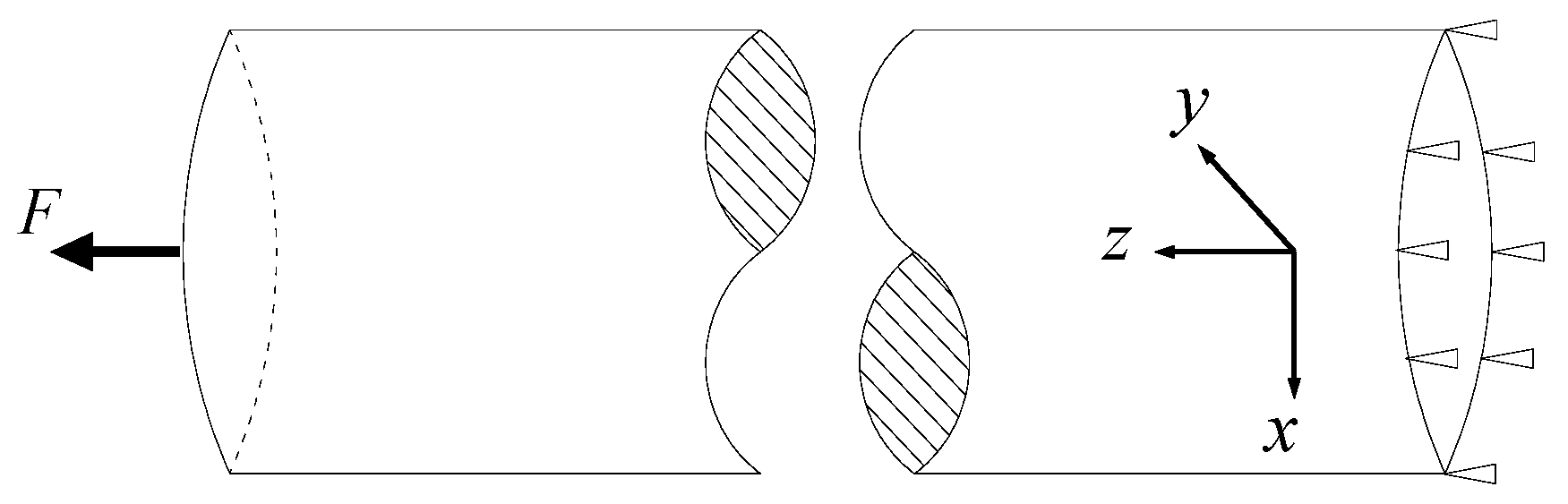
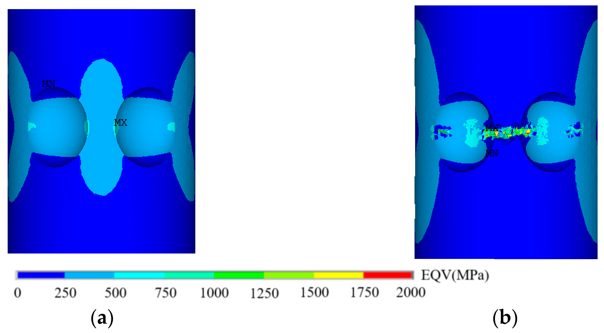
To comprehensively assess the impact of fatigue loads and morphological changes in corrosion pits on the mechanical performance and fatigue life of steel structures, scholars have proposed the application of continuous damage mechanics to establish a fatigue damage model for predicting fatigue life [11]. This method considers corrosion pits on the surface of steel wires as notches rather than cracks. Through iterative computations of the cumulative damage incurred by the wire, the corrosion pit model state is updated, thereby achieving the objective of accounting for morphological changes in corrosion pits. To further address practical engineering environments and the influence of multiple corrosion pits on the damage evolution process, this study innovatively integrated a traffic–bridge–wind simulation analysis model. The research systematically investigated the fatigue-damage evolution patterns of single and double corrosion pits in suspension bridge cables. Based on the principles of continuous damage mechanics theory, a damage evolution model for high-strength steel wires was meticulously developed within the finite element software ANSYS. Using the life and death element method, the intricate process of damage evolution in wires under single pit conditions and various pit distribution forms was simulated. This simulation not only visually elucidated the progression of damage at corrosion pits but also facilitated a comprehensive analysis of the stress state and fatigue life of high-strength steel wires.

2. The Continuous Damage Mechanics Model

Based on the concept of continuum damage mechanics, the failure process of materials can be described by the damage variable D. For the high-strength steel wire studied in this study, the damage variable is regarded as the gradual loss of effective area. Its formulation is expressed as follows:

$$D=\frac{S_D}{S}$$

(1)

where S represents the area of a cross-section of a specific volume element of the steel wire, determined by its normal; S_D is the defect area on that cross-section.

According to Formula (1), the effective stress σ_e generated by the action of external force F can be defined as:

$${\sigma }_e=\frac{\sigma }{1-D}$$

(2)

where σ represents the nominal stress.

2.1. Elastic–Plastic Damage Model

Adopting the simplified model proposed by Sun [12], this model was derived from the simplified version of the Chaboche [13] elastic damage model. It is used for computing the loss in the effective cross-sectional area. The simplified model is expressed as follows:

$$d{D}_e=D^{\alpha }\cdot {\left[\frac{{\sigma }_a}{2M_0}\right]}^{\beta }dN$$

(3)

where D_e represents elastic fatigue damage; σ_a represents stress amplitude; N represents cycle numbers; α, β and M₀ are coefficients of the fatigue damage law [13].

By solving Equation (3), the relationship between elastic fatigue damage D_e and the number of cycles N can be obtained:

$$D_{\mathrm{e}}(N)={\left[(1-\alpha ){\left[\frac{{\sigma }_a}{2M_0}\right]}^{\beta }N\right]}^{\frac{1}{1-\alpha }}$$

(4)

Based on the experimental data [14], the material parameters can be determined as follows: M₀ = 5740 MPa, α = 0.75, β = 2.97.

Lemaitre [13] proposed a ductile damage evolution model based on plastic strain. This model can be extended to calculate incremental fatigue damage caused by plastic strain. The cumulative damage calculation for each cycle is as follows:

$$d{D}_p={\left[\frac{{({\sigma }_{\max }^{*})}^2}{2ES{(1-D)}^2}\right]}^m\Delta \epsilon \cdot dN$$

(5)

where D_p represents plastic fatigue damage; σ*_max is the maximum value of the damage equivalent stress; E represents Young’s modulus; S (MPa) and m are the two characteristic creep damage coefficients for the material; Δε is the accumulated plastic strain.

Due to the lack of reliable experimental data, the plastic fatigue damage evolution equation proposed by Cui et al. [14] is used:

$$d{D}_p=(1+\frac{\Delta \epsilon }{\epsilon })\cdot D^{\alpha }\cdot {\left[\frac{{\sigma }_a}{2M_0}\right]}^{\beta }dN$$

(6)

where ε is the maximum elastic strain.

2.2. Load Block Method

Typically, the lifespan of bridge cables made of high-strength steel wires is relatively long, and the cumulative damage of the wires under load cycles is relatively low. It is both time-consuming and unnecessary to calculate the damage for each load cycle. Therefore, it is common to establish a cyclic load region to accelerate the algorithmic process for simulating corrosion fatigue damage [15,16]. Specifically, assuming the material’s damage rate δD/δN remains constant over ΔN cycles, these ΔN cycles are treated as a cyclic load block, as illustrated in Figure 1. Consequently, the damage increment for each load block can be calculated using the following formula:

$$\Delta D={\left(\frac{\delta D}{\delta N}\right)}_i\times \Delta N$$

(7)

Considering that the accuracy of the cyclic load block directly influences the precision of the results, seven sets of scenarios with cyclic load region accuracies ranging from 0.3 years to 0.9 years were calculated. It was observed that the average calculated result was approximately 68 years, with a difference of less than 3% compared to the result obtained with the minimum accuracy (as shown in

Table 1. Calculation results under different precisions of load block.

Cyclic Accuracy (Year)	Results (Year)
0.3	66.0
0.4	67.6
0.5	68.0
0.6	69.0
0.7	70.0
0.8	68.0
0.9	72.0

). Therefore, taking into account the requirements for both computational efficiency and accuracy, a cyclic load block accuracy of 0.5 years was selected for this study.

After calculating ΔD_e and ΔD_p for each cycle based on Equations (3) and (6), the damage variable D_t after that cycle can be determined using Equations (8) and (9). Using this data, the material parameters for the steel wire are updated to simulate the degradation of material performance, achieving the effect of material deterioration.

$$\Delta D_t^{i+1}=Max\left\{\Delta D_e^{i+1},\Delta D_p^{i+1}\right\}$$

(8)

$$D_t^{i+1}=D_t^i+\Delta D_t^{i+1}$$

(9)

where $\mathsf{\Delta }{D}_t^i$ represents the damage increment obtained from the calculation of the i-th cyclic load block.

3. Finite Element Simulation

Integrating the aforementioned concepts, the element birth and death technique in ANSYS is used to simulate the damage of the steel wire. The damage variable D is assigned to each element, and when D reaches 1, the element is considered fully damaged. The element birth and death technique is used to deactivate such elements, rendering them inactive for subsequent calculations. The cycle at which the damage variable D of the first element reaches the critical value is considered as the crack initiation life. When a substantial amount of damage occurs around the pit and the simulation results no longer converge, the wire is regarded as completely damaged, and the accumulated cycles at this point are considered as the fatigue life of the wire. The use of the element birth and death technique allows for a better consideration of the interaction between pit cracks and pit damage, and provides a visual representation of crack formation at the pit. The flow chart of the fatigue-damage evolution procedure is shown in Figure 2.

3.1. Finite Element Model

For the pit in a finite element simulation, there is no need to adopt complex random geometric shapes. A simple spherical shape is sufficient for accurate fatigue life predictions [11]. Based on the experimental results of CERIT et al. [17], a semi-ellipsoidal pit model was used to simulate the pit shape. On the basis of analyzing a single-pit wire, two relative position distributions of pits on the wire are discussed: along the Z-axis and along the X-axis, as illustrated in Figure 3.

The accuracy and computational efficiency of the finite element model are influenced by the shape and density of the mesh. Therefore, it is crucial to partition the mesh reasonably. Considering the stress distribution characteristics of steel wire with pits, this paper adopts a regional partitioning method. More refined mesh partitioning is applied to the damage-sensitive pit areas to meet the requirements for accurate calculation of damage evolution analysis at the pit. The mesh size in the regions far from the pits on both ends of the wire can be appropriately increased to improve computational efficiency.

After element mesh, the calculated elemental stress and nodal stress consistently differ. However, if the disparity is too significant, it indicates insufficient refinement in the meshing at that location [18]. Based on this concept, Wu et al. [19] used the error values between calculated elemental stress and nodal stress to validate the adequacy of mesh refinement. To verify the correctness of the element mesh, different mesh accuracies are applied to partition the pit area of the steel wire, and calculations are performed separately. Finally, a comparison is made between the maximum element stress (S_E) and the maximum node stress (S_N). It is generally considered that the mesh partitioning is reasonable if the deviation between the two is within 5%. The calculation results are shown in

Table 2. Comparison of maximum element stress and maximum node stress under different meshes.

Mesh Accuracy (mm)	SE (MPa)	SN (MPa)	SE/SN (%)
0.4	968.24	1055.12	91.77
0.2	996.95	1066.67	93.46
0.1	1019.91	1062.04	96.03
0.05	1041.12	1063.03	97.93

.

Considering the trade-off between computational cost and accuracy requirements, a mesh size of 0.1 mm is chosen for the area around the pit, while the element size at both ends of the wire is set to 0.4 mm. The mesh of the element is illustrated in Figure 4.

3.2. Boundary Conditions

A solid model of corroded steel wire was established by using the finite element software ANSYS 2020R2. Considering the requirements for solution accuracy and computational efficiency, the SOLID95 element was selected to build a solid model of corroded steel wire.

Given that the steel wire is mainly subjected to axial tension, a loading method is adopted where axial face tensile stress is applied at one end of the steel wire, and the other end is fixed, as shown in Figure 5. A cylinder with a diameter of 5.25 mm is used to simulate the steel wire, and the pit is located in the middle of the wire. The length of the steel wire solid model is set to 20 mm. The basic parameters of the model are shown in

Table 3. Key parameters of finite element model of the steel wire.

Elastic Modulus (GPa)	Poisson’s Ratio	Element Type	Tensile Strength (MPa)	Density (kg·m−3)
206	0.3	SOLID95	1670	7850

.

4. Method Verification

To validate the effectiveness of the steel wire elastic–plastic damage evolution model established in ANSYS, experimental data from Jiang et al. [20] were collected. Simulations were performed on specimens suitable for elastic–plastic fatigue damage analysis.

In the experiments [20], several single-pit galvanized high-strength steel wire specimens were produced using an accelerated corrosion device. The corrosion fatigue behavior of pre-corroded steel wire was studied through fatigue tests. In this section, three high-strength steel wire models with the same experimental parameters were established in ANSYS (as shown in

Table 4. Parameter table of mechanical properties of corrosion fatigue test specimens.

Ultimate Strength (MPa)	Yield Strength (MPa)	Elastic Modulus (GPa)
1672	1473	206

); the test specimens are numbered F1, F2, F3, respectively. The fatigue life of pre-corroded high-strength steel wire in a dry environment was calculated based on the elastic–plastic damage evolution model and compared with the experimental results, as shown in

Table 5. Comparison between fatigue test data and numerical simulation results.

Code	Maximum Stress (MPa)	Stress Ratio	Frequency (Hz)	Fatigue Life in Tensile Testing (Times)	Numerical Simulation Fatigue Life (Times)	Error
F1	1200.5	0.167	30	128,564	115,000	10.6%
F2	960.4			199,723	160,000	19.9%
F3	720.3			425,827	375,000	11.9%

. The average error is approximately 14.13%.

Zhang et al. [21] used both fracture mechanics and continuous damage mechanics methods to calculate the fatigue life of pitted steel bar. A comparison revealed that when the simulation results had an error of approximately 20% compared to the experimental results, this predictive method demonstrated good applicability. In summary, the calculated results of this study are in good agreement with the tensile test results, demonstrating that the numerical simulation method adopted in this paper can effectively simulate the damage evolution process of pre-corroded steel wire.

5. Wind–Traffic–Bridge Coupled System

In order to simulate the stress environment of the suspension cable wire more realistically, we adopt the stress–time history of the suspension cable obtained from the wind–traffic–bridge coupled system analysis [22] as the loading condition in this paper.

The wind–traffic–bridge coupled system refers to a time-varying system under the action of dual random excitations (traffic and pulsating wind). It mainly involves two aspects of coupling: the fluid–structure coupling between strong wind and the bridge, and the solid contact coupling between traffic and the bridge. The wind–traffic–bridge coupled system [22] used in this study is based on a simulation platform established using the finite element method. This platform systematically considers the dynamic interactions between the bridge structure, random wind, and traffic. The system mainly consists of two subsystems: vehicle–bridge and wind–bridge. The entire simulation process involves three steps: first, the numerical models of the bridge and vehicles are established to obtain the mass and stiffness matrices in ANSYS; second, the simulation of stochastic wind field and traffic conditions is conducted to calculate the wind loads acting on the bridge and vehicles, as well as the interaction forces between them; finally, the control equations for the wind–traffic–bridge coupled vibration system are established, as shown in Equation (10), and the dynamic analysis of the wind–traffic–bridge coupled system is carried out in MATLAB 2019b.

$$\begin{array}{l}\left[\begin{array}{cccc}{M}_b& 0& \cdots & 0\\ 0& M_{v1}& \cdots & 0\\ ⋮& ⋮& \ddots & ⋮\\ 0& 0& \cdots & M_{vn}\end{array}\right]\left\{\begin{array}{c}{\ddot{q}}_b\\ {\ddot{q}}_{v1}\\ ⋮\\ {\ddot{q}}_{vn}\end{array}\right\}+\left[\begin{array}{cccc}{C}_b& 0& \cdots & 0\\ 0& C_{v1}& \cdots & 0\\ ⋮& ⋮& \ddots & ⋮\\ 0& 0& \cdots & C_{vn}\end{array}\right]\left\{\begin{array}{c}{\dot{q}}_b\\ {\dot{q}}_{v1}\\ ⋮\\ {\dot{q}}_{vn}\end{array}\right\}+\left[\begin{array}{cccc}{K}_b& 0& \cdots & 0\\ 0& K_{v1}& \cdots & 0\\ ⋮& ⋮& \ddots & ⋮\\ 0& 0& \cdots & K_{vn}\end{array}\right]\left\{\begin{array}{c}{q}_b\\ q_{v1}\\ ⋮\\ q_{vn}\end{array}\right\}=\\ \left\{\begin{array}{c}({\displaystyle {\sum }_{i=1}^n{F}_{vi}^G})+F_b^R+F_b^C+F_b^{Se}+F_b^{Bu}\\ F_{v1}^R+F_{v1}^C+F_{v1}^W\\ ⋮\\ F_{vn}^R+F_{vn}^C+F_{vn}^W\end{array}\right\}\end{array}$$

(10)

where n represents the total number of vehicles in the traffic flow; q represents the displacement vector; M represents the mass matrix of the structure; C represents the damping matrix; K represents the stiffness matrix; F is the force matrix; subscripts b and vi (i = 1, 2, 3, ..., n) represent the bridge system and the i-th vehicle, respectively; superscripts G, R, C, W, Se, and Bu represent the excitation loads corresponding to gravity, road roughness excitation, vehicle–bridge coupled interaction, static wind, self-excitation, and buffeting force.

By solving the wind–traffic–bridge coupled control equations, the stress vector can be further calculated based on the deflection–strain relationship and the stress–strain relationship, as shown in the following equation:

$$\left[S\right]=\left[E\right]\left[B\right]\left\{q_b\right\}$$

(11)

where [S] is the predicted stress vector; [E] is the stress–strain relationship matrix; [B] is the stress–deflection relationship matrix derived from the shape functions of the element; q_b is the displacement vector.

The stress data of the beam end suspension cable S1 under different loading conditions obtained from the wind–traffic–bridge coupled system [22] are used to calculate the estimated effective stress range and the daily average number of cycles for the S1 suspension cable, as shown in

Table 6. Predicted effective stress range and average daily number of cycles.

Suspender	Estimated Effective Stress Range	Estimated Daily Average Number of Cycles
S1	13.32	7278

.

Combining the data from Table 5, using the rain-flow counting method to process the stress time history of the S1 suspension cable under this loading condition, a sinusoidal function can be obtained to represent the alternating load applied to the end of the steel wire, as shown in the following equation:

$${\sigma }_t={\sigma }_0+{\sigma }_a\sin (\frac{2\mathsf{\pi }}{T}t)=243+13.32\sin (\frac{\mathsf{\pi }t}{6})$$

(12)

where σ_t is the stress value corresponding to the time t; σ₀ is the mean stress; σ_a is the stress amplitude; t is the loading time.

6. The Impact of Pitting Distribution on the Damage Evolution of Steel Wire

Based on the finite element model and loading conditions established in the previous sections, this section explores the relationship between the dual-pit position distribution and the mechanical properties, as well as the fatigue life of the steel wire. A comparative analysis was conducted with the results obtained for the single-pit steel wire.

6.1. Damage Evolution Model for Single-Pit Steel Wire

Using the theoretical methods outlined in Section 1 and Section 2, finite element calculations were conducted. Figure 6 illustrates the stress contour plots for the occurrence of damage and complete failure in a single-pit scenario. As depicted in Figure 6a, the first fully damaged element appeared in the 56th year. The stress distribution path in Figure 6 clearly indicates the stress state at the pit, and the position of the damaged element is closely related to the high-stress region. Figure 7 provides stress paths along the X and Z axes at the pit, clearly indicating the high-stress state at the pit. Under cyclic loading, the damage gradually spreads from both sides to the bottom of the pit, forming a damage band at the pit, as shown in Figure 6b. Despite the entire process taking 68 years from the start of loading to complete damage, the time from crack initiation to wire failure is only approximately 13 years, constituting 19.1% of the entire fatigue life. This highlights the nonlinear nature of damage evolution at the wire pit (as shown in Figure 8), with crack initiation significantly accelerating crack propagation until wire failure.

6.2. The Influence of Dual Pits on the Stress Distribution in Steel Wire

When multiple pits are present on the steel wire, changes in their relative positions can affect the stress concentration locations and the degree of stress concentration. This, in turn, leads to variations in the time of crack nucleation and the evolution pattern of damage. In this section, the relationship between the relative distribution positions of dual pits and the stress distribution in the steel wire is explored through extensive finite element simulations.

6.2.1. Dual Pits Distributed along the X-Axis on the Surface of Steel Wire

When dual pits are distributed along the X-axis, the spacing between the pits is represented by the angle θ, as shown in Figure 3a. When the pits intersect (θ = 30°), damage first occurs at the intersection of the dual pits. This is because the surface angle at this point leads to more severe stress concentration, and the damage accumulation rate reaches its highest when the edges of the pits are tangential. Therefore, the first visible damage occurred as early as the 15th year (as shown in Figure 9a), which is 31 years earlier compared to the single-pit wire. When the dual pits are separated (θ = 60°), the high-stress zones are distributed on both sides of the edges of the two pits, and the stress on the side where the pits are closer is higher than that on the farther side, as shown in Figure 10 and Figure 11. Compared to the cases where the pits intersect or are tangential, the stress concentration phenomenon is weakened when the pits are separated, but it is still stronger than the single-pit case. This is because even when the pits are separated, the distance between them is still relatively close, and there is a cumulative trend in the damage of the two pits. As the pits are farther apart, i.e., as θ approaches 180°, the stress distribution and damage accumulation rate become closer to the single-pit case, as demonstrated in the subsequent cases.

6.2.2. Dual Pits Distributed along the Z-axis on the Surface of Steel Wire

When dual pits are distributed along the Z-axis, their relative positions are represented by the longitudinal distance l between pits and the pit radius a, as shown in Figure 3b. The intersection and separation of pits along the Z-axis are illustrated in Figure 12 and Figure 13, respectively. Figure 14 reveals the surface stress distribution near the pits. Compared to Figure 11 and Figure 14, the stress variation near the pits is smaller, and the rate of damage occurrence is slower. The reasons for these results can be attributed to the following two points: (1) Since the high-stress zones of the pits are distributed along the X-axis, the Z-axis intersection of dual pits does not result in the overlap of high-stress zones. Therefore, the damage accumulation of the pits does not overlap at this time. (2) Dual pits intersecting along the Z-axis can be regarded as a large pit with a large aspect ratio. This type of pit, when subjected to axial tensile stress, has a lower stress concentration effect than a general ellipsoidal pit [19]. This explains why the damage accumulation of dual pits intersecting along the Z-axis is slower than that of a single pit. When the pits along the Z-axis are tangential or separated, the stress distribution pattern is similar to that of the intersection, and as the distance between pits increases, it approaches the situation of a single pit.

6.3. The Influence of Dual Pits on Fatigue Life

In the light of the damage model established in Section 2, the fatigue damage evolution process under different conditions was simulated in ANSYS. As shown in Figure 15a, when the pits intersect along the X-axis, the cumulative damage rate of wire elements accelerates with the increase in the pit angle, reaching its maximum as the pits approach tangency. When the pits no longer intersect, the cumulative damage rate of wire elements significantly decreases and continues to decrease with the increase in the pit angle θ. Figure 16a illustrates that when dual pits intersect, the fatigue life of the wire is much lower than that of a single-pit wire, decreasing further as the pits approach tangency. When the dual pits are tangential, the wire’s fatigue life reaches a minimum of 19.5 years, reduced by approximately 71.9% compared to a single-pit wire under the same loading conditions. As the relative position of dual pits gradually becomes separate, the fatigue life of the wire increases.

As shown in Figure 15b, when the pits intersect along the Z-axis longitudinally and the pit spacing l does not exceed the pit radius a (i.e., l/a < 1), the cumulative damage rate of the wire elements decreases with the increase in l and remains consistently lower than that of a single-pit wire until l = a, where the damage evolution rate reaches its minimum. However, when l/a > 1, the cumulative damage rate of the wire elements begins to increase with the increase in l and gradually approaches that of a single-pit wire. Figure 16b reveals the pattern of dual-pit wire fatigue life as the l/a ratio varies: when l/a < 1, the wire’s fatigue life is significantly higher than that of a single-pit wire, increasing with the pit spacing l but with minimal increments. When l/a = 1, the wire’s fatigue life reaches its maximum, increasing by about 15.1% compared to a single-pit wire. When l/a > 1, the wire’s fatigue life begins to decrease with the increase in pit spacing l, gradually approaching that of a single-pit wire.

7. Conclusions

In this study, an elastic–plastic damage constitutive model and an elastic–plastic damage evolution model for high-strength steel wires were established based on continuum damage mechanics. The wire elements of a suspension rod in a certain cable-stayed bridge were taken as the research object. The finite element software ANSYS was used to analyze the damage evolution behavior under the coupling effects of traffic flow, bridge, and wind. Furthermore, the reliability of the simulation results was verified using experimental data from the literature. Considering the possibility of multiple pits in corroded steel wires in practical engineering, this study, based on the damage evolution model, explored the influence of the relative distribution of pits on the mechanical properties and fatigue life of the wire. The specific conclusions are as follows:

1. Based on the theory of continuous damage mechanics, the element birth and death technique was used to simulate the damage evolution process of pitted steel wire in ANSYS. This approach better accounts for the interaction between damage-induced pits and cracks as well as the effects of stress concentration. The model’s calculated results demonstrated good agreement with experimental results under similar conditions, validating the rationality of this method.

2. For single-pit steel wires, after the initiation of cracks, cracks at the pit site will rapidly propagate and accelerate the failure of the steel wire. The crack initiation life constitutes approximately 80% of the steel wire’s fatigue life under high-cycle fatigue conditions. This indicates that under high-cycle fatigue, the crack initiation life dominates the majority of the fatigue life.

3. Using the wind–traffic–bridge coupling system calculated stress–time history data as the load condition, we thoroughly discussed the influence of the relative distribution position of pits on the mechanical properties and fatigue life of steel wires. When pits are distributed along the X-axis of the wire, the intersection of pits leads to the overlap of stress concentration zones, resulting in the superposition of fatigue damage at the pit locations and ultimately accelerating the fatigue failure of the steel wire. Moreover, the fatigue life of the steel wire is minimized when the pits are tangential. When pits are distributed along the Z-axis of the wire, the pits formed by the intersection have a larger aspect ratio. This shape of pits, compared to semi-ellipsoidal pits, has a lower stress concentration, thereby slowing down the rate of damage accumulation at the pit locations. Therefore, even with a higher number of surface pits, the steel wire exhibits a higher fatigue life than a single-pit steel wire. When the distance between pits equals the pit radius, the steel wire achieves the maximum fatigue life. The above results indicate that different pit distribution states significantly affect the fatigue life of the steel wire, providing theoretical reference for the maintenance and normal operation of cable structures.

References

1. Zhou, J.T.; Xia, R.C.; Zhang, H. Research and application of bridge internal steel structure disease detection. J. Chongqing Jiaotong Univ. (Nat. Sci.) 2021, 40, 20–28. (In Chinese) [Google Scholar] [CrossRef]
2. Zhang, H.; Yuan, Y.; Xia, R.C.; Zhou, J.T.; Chen, Y. Research progress of stay cable disease detection robot. J. Chongqing Jiaotong Univ. (Nat. Sci.) 2022, 41, 59–62. (In Chinese) [Google Scholar] [CrossRef]
3. Zhou, J.H.; Yang, Q.M. Corrosion mechanism and finite element analysis of single steel wire of stay-cable. Low Temp. Archit. Technol. 2016, 38, 69–72. (In Chinese) [Google Scholar] [CrossRef]
4. Wang, G.; Ma, Y.; Guo, Z.; Bian, H.; Wang, L.; Zhang, J. Fatigue life assessment of high-strength steel wires: Beach marks test and numerical investigation. Constr. Build. Mater. 2022, 323, 126534. [Google Scholar] [CrossRef]
5. Sankaran, K.K.; Perez, R.; Jata, K.V. Effects of pitting corrosion on the fatigue behavior of aluminum alloy 7075-T6: Modeling and experimental studies. Mater. Sci. Eng. 2001, 297, 223–229. [Google Scholar] [CrossRef]
6. Wang, Y.; Zheng, Y.Q.; Zhang, W.H.; Lu, Q.R. Analysis on damage evolution and corrosion fatigue performance of high-strength steel wire for bridge cable: Experiments and numerical simulation. Theor. Appl. Fract. Mech. 2020, 107, 102571. [Google Scholar] [CrossRef]
7. Amiri, M.; Arcari, A.; Airoldi, L.; Naderi, M.; Iyyer, N. A continuum damage mechanics model for pit-to-crack transition in AA2024-T3. Corros. Sci. 2015, 98, 678–687. [Google Scholar] [CrossRef]
8. Hu, W.P.; Shen, Q.A.; Zhang, M.; Meng, Q.C.; Zhang, X. Corrosion–fatigue life prediction for 2024-T62 aluminum alloy using damage mechanics-based approach. Int. J. Damage Mech. 2012, 21, 1245–1266. [Google Scholar] [CrossRef]
9. Zhao, Y.; Su, B.; Fan, X.; Yuan, Y.; Zhu, Y. Corrosion Fatigue Degradation Characteristics of Galvanized and Galfan High-Strength Steel Wire. Materials 2023, 16, 708. [Google Scholar] [CrossRef]
10. Tang, S.; Xu, H.; Ao, N.; Liu, Y.; Zhang, J.; Guo, H.; Kan, Q.; Kang, G.; Wu, S. Experimental investigation on corrosion fatigue crack initiation and growth of heat-treated U75V rail steel. Int. J. Fatigue 2023, 178, 107973. [Google Scholar] [CrossRef]
11. Khajeian, A.; Mahmoudi, A.H.; Seif, R. An approach to predicting corrosion fatigue for marine applications. Int. J. Fatigue 2023, 179, 108030. [Google Scholar] [CrossRef]
12. Sun, B. A continuum model for damage evolution simulation of the high strength bridge wires due to corrosion fatigue. J. Constr. Steel Res. 2018, 146, 76–83. [Google Scholar] [CrossRef]
13. Lemaitre, J.; Chaboche, J.L.; Maji, A.K. Mechanics of Solid Materials; Cambridge University Press: Cambridge, UK, 1990; pp. 349–371. [Google Scholar]
14. Cui, C.J.; Chen, A.R.; Ma, R.J. An improved continuum damage mechanics model for evaluating corrosion–fatigue life of high-strength steel wires in the real service environment. Int. J. Fatigue 2020, 135, 105540. [Google Scholar] [CrossRef]
15. Hu, P.; Meng, Q.; Hu, W.; Shen, F.; Zhan, Z.; Sun, L. A continuum damage mechanics approach coupled with an improved pit evolution model for the corrosion fatigue of aluminum alloy. Corros. Sci. 2016, 113, 78–90. [Google Scholar] [CrossRef]
16. Shen, F.; Hu, W.P.; Meng, Q.C. A damage mechanics approach to fretting fatigue life prediction with consideration of elastic-plastic damage model and wear. Tribol. Int. 2015, 82, 76–90. [Google Scholar] [CrossRef]
17. Cerit, M.; Genel, K.; Eksi, S. Numerical investigation on stress concentration of corrosion pit. Eng. Fail. Anal. 2009, 16, 2467–2472. [Google Scholar] [CrossRef]
18. Chang, K.H.; Choi, K.K. An error analysis and mesh adaptation method for shape design of structural components. Comput. Struct. 1992, 44, 1275–1289. [Google Scholar] [CrossRef]
19. Wu, M.X.; Yin, L.; Tang, D.F. Influence of corrosion pit size on stress concentration of high strength steel wire. J. Southwest Pet. Univ. (Sci. Technol. Ed.) 2021, 43, 63–70. (In Chinese) [Google Scholar] [CrossRef]
20. Jiang, J.H.; Ma, A.B.; Weng, W.F.; Fu, G.H.; Zhang, Y.F.; Liu, G.G.; Lu, F.M. Corrosion Fatigue Performance of Pre-Split Steel Wires for High Strength Bridge Cables. Fatigue Fract. Eng. Mater. Struct. 2009, 32, 769–779. [Google Scholar] [CrossRef]
21. Zhang, F.; Jin, W.L.; Zhang, J.; Mao, H.Y.; Fan, W.J. Numerical Analysis of High Cycle Fatigue Damage and Life of Pitted Corroded Steel Bar Based on Continuum Damage Mechanics. J. Build. Mater. 2021, 24, 405–411. (In Chinese) [Google Scholar] [CrossRef]
22. Wu, M.; Zhu, J.; Heng, J.; Kaewunruen, S. Fatigue assessment on suspenders under stochastic wind and traffic loads based on in-situ monitoring data. Appl. Sci. 2019, 9, 3405. [Google Scholar] [CrossRef]
Figure 1. Schematic diagram of the relationship between load block, analysis step and the number of cyclic loads. (a) The relationship between cyclic loads and load block; (b) Loading of load block.
Applsci 14 02015 g001
Figure 2. The schematic diagram of corrosion pit.
Applsci 14 02015 g002
Figure 3. The schematic diagram of corrosion pit. (a) Pit distribution along the X-axis on the surface of the steel wire; (b) Pit distribution along the Z-axis on the surface of the steel wire.
Applsci 14 02015 g003
Figure 4. Mesh of the finite element model.
Applsci 14 02015 g004
Figure 5. Schematic diagram of boundary conditions with applied load.
Applsci 14 02015 g005
Figure 6. Stress nephogram of single-pit steel wire at different time points. (a) 56th year; (b) 68th year.
Applsci 14 02015 g006
Figure 7. Stress path along different directions at the corrosion pit. (a) Along the X-axis direction; (b) Along the Z-axis direction.
Applsci 14 02015 g007aApplsci 14 02015 g007b
Figure 8. Damage variable curve.
Applsci 14 02015 g008
Figure 9. Stress nephogram of double-pits on steel wire at different time points (θ = 30°). (a) 15th year; (b) 29.5th year.
Applsci 14 02015 g009
Figure 10. Stress nephogram of double-pits on steel wire at different time points (θ = 60°). (a) 15th year; (b) 50.5th year.
Applsci 14 02015 g010
Figure 11. Stress path along X-axis at the corrosion pit. (a) θ = 30°; (b) θ = 60°.
Applsci 14 02015 g011aApplsci 14 02015 g011b
Figure 12. Stress nephogram of double-pits on steel wire at different time points (l/a = 1). (a) 50th year; (b) 80th year.
Applsci 14 02015 g012
Figure 13. Stress nephogram of double-pits on steel wire at different time points (l/a = 3). (a) 50th year; (b) 65.5th year.
Applsci 14 02015 g013
Figure 14. Stress path along Z-axis at the corrosion pit. (a) l/a = 1; (b) l/a = 3.
Applsci 14 02015 g014
Figure 15. Damage variable curves under different pit distribution positions. (a) Along the X-axis; (b) Along the Z-axis.
Applsci 14 02015 g015
Figure 16. The relationship between fatigue life of steel wire and corrosion pit distribution. (a) Along the X-axis; (b) Along the Z-axis.
Applsci 14 02015 g016