Abandoned Farmland Extraction and Feature Analysis Based on Multi-Sensor Fused Normalized Difference Vegetation Index Time Series—A Case Study in Western Mianchi County

Abstract

Farmland abandonment monitoring is one of the key aspects of land use and land cover research, as well as being an important prerequisite for ecological environmental protection and food security. A Normalized Difference Vegetation Index (NDVI) time series analysis is a common method used for farmland abandonment data extraction; however, extracting this information using high-resolution data is still difficult due to the limitations caused by cloud influence and data of low temporal resolution. To address this problem, this study used STARFM for GF-6 and Landsat 8 data fusion to enhance the continuity of high-resolution and cloudless images. A dataset was constructed by combining the phenological cycle of crops in the study area and then extracting abandoned farmland data based on an NDVI time series analysis. The overall accuracy of the results based on the NDVI time series analysis using the STARFM-fused dataset was 93.42%, which was 15.5% higher than the accuracy of the results obtained using only GF-6 data and 28.52% higher than those obtained using only Landsat data. Improvements in accuracy were also achieved when using SVM for time series analysis based on the fused dataset, indicating that the method used in this study can effectively improve the accuracy of the results. Then, we analyzed the spatial distribution pattern of abandoned farmland by extracting the results and concluded that the abandonment rate increased with the increase in the road network density and decreased with the increase in the distance to residential areas. This study can provide decision-making guidance and scientific and technological support for the monitoring of farmland abandonment and can facilitate the analysis of abandonment mechanisms in the study area, which is conducive to the sustainable development of farmland.

1. Introduction

Farmland abandonment is one of the key aspects of land use and land cover (LULC) research [1,2]. The phenomenon of farmland abandonment in China has become increasingly serious due to accelerated urbanization, industrialization, land pollution, the loss of labor, and other anthropogenic and natural factors [3,4,5]. The aggravation of the phenomenon of farmland abandonment harms ecological safety, food security, and agricultural stability [6,7,8]. Therefore, the detection of abandoned farmland is of great significance for ecological and environmental protection, food security, and agricultural stability. Mianchi County, Sanmenxia City, Henan Province, a typical agricultural county in China, is rich in farmland resources. However, due to insufficient governmental management, farmland abandonment is common and is detrimental to food production and farmland resources [9]. Therefore, there is an urgent need to strengthen the government’s management and supervision of the phenomenon of farmland abandonment.

Farmland abandonment is defined as a period of time in which there is no human cultivation activity on farmland. Some studies consider that no cultivation activity in a single season can be defined as abandonment [10], but most studies define it as farmland with no cultivation activity for two consecutive years or more, distinguishing between seasonal and permanent abandonment based on duration [11,12]. The traditional method used for monitoring abandoned farmland is field surveys [13,14], which require a considerable amount of human and material resources and are unsuitable for large-scale, high-precision, or long-term projects [15]. With the popularization of remote-sensing technology, the interpretation and analysis of remote-sensing images have become a common and effective method for monitoring farmland abandonment [16,17]. Alcantara et al. used the MODIS Normalized Difference Vegetation Index (NDVI) series to identify abandoned farmland using SVM [16]. Xiao et al. used the CART decision tree for extraction and explored the spatial distribution pattern of abandoned farmland [12]. Löw et al. and Wei et al. identified abandonment through random forest modeling based on changes in the vegetation index (VI), achieving good accuracy [18,19]. Most of these methods were based on multi-temporal remote-sensing image interpretation, which can extract abandoned farmland data and distinguish between seasonal and permanent abandonment. However, due to the phenomena of “different spectrums with the same object” and the “same spectrums with the same object”, the extraction results are easily interfered with by shrubs and weeds, and when the number of images increases, the cumulative error also increases, resulting in a loss of accuracy. The NDVI is one of the important parameters reflecting the growth of crops. The change in the NDVI between the growing and non-growing stages of artificial crops is more obvious than that of natural vegetation; thus, according to this principle, we can distinguish abandoned farmland well. Wu et al. and Chen et al. extracted abandoned farmland information based on an NDVI time series analysis and obtained highly accurate results [20,21]. Wang et al. used block-level vector-boundary-based time series analysis to extract data regarding abandoned farmland in cloudy and rainy areas [22]. Lee et al. plotted the change curves of multi-VI time series and combined them with harmonic analysis for abandonment extraction [23]; this kind of method, based on time series analysis, can alleviate the influence of shrubs and weeds but cannot distinguish between seasonal abandonment and permanent abandonment. To address the shortcomings of the above two methods, Song et al. combined decision trees based on time series analysis. Their method weakened the impact of weeds and shrubs in time series analysis and distinguished between seasonal and permanent abandonment [24].

In all of the above studies, the accuracy of the extraction results depended on the resolution of the remote-sensing images [25]. Therefore, due to the popularization of high-resolution remote-sensing images, we selected these as the data source for abandoned farmland data extraction. Li et al. and Luo et al. chose GF-1 and GF-6 as the data sources in their studies, and the overall accuracy was higher than for middle- and coarse-resolution-image-based results [26,27]. However, due to the low temporal resolution of these images, it is often difficult to obtain continuous remote-sensing images that can cover the whole study area, making it difficult to construct a time series dataset. To address this problem, spatial–temporal resolution fusion techniques are widely used, which can be mainly categorized into methods based on pixel unmixing (MMT [28], STRUM [29], etc.), methods based on weighting functions (STARFM [30], ESTARFM [31], etc.), and algorithms combining the two methods (FSDAF [32], EFSDAF [33], etc.). Pixel unmixing often requires high-resolution land classification data, while enhanced algorithms based on STARFM usually require multiple pairs of high- and low-resolution image pairs, and when faced with the rainy season, it can be difficult to collect data. However, the STARFM algorithm only needs a pair of images of high and low spatial resolution obtained at similar times to predict high-spatial-resolution images at another time, which is less demanding than other methods and, thus, has been widely used to construct time series datasets for analysis. Zhang et al. used STARFM to fuse MODIS and Landsat images to improve the accuracy of the replanting index extracted using time series analysis [34]. Zhang et al. and Schmidt et al. used a STARFM-fused dataset to estimate the biomass trend of alpine grassland and monitor the dynamics of forest destruction and regeneration [35,36]. Kong et al. fused GF-1 and MODIS data to differentiate between cultivated and abandoned farmland and to further differentiate crop types [37]. The above research applications show that the STARFM algorithm can reduce the difficulty of time series dataset construction when selecting high-resolution remote sensing images as a single source and can enhance the accuracy of the extraction results through time series analysis.

To address the problems with the methodology mentioned above, this study took western Mianchi County as the study area and supplemented the time stamp without GF-6 data covered by STARFM-fused data, which alleviated the problem of no data coverage in the growing and non-growing stages of some crops that would have resulted in reduced accuracy. Then, the NDVI time series analysis was combined with overlay analysis to extract abandoned farmland data from 2021 and 2022 in the study area, and a distinction was made between seasonal and permanent abandonment. Finally, the features of the abandoned farmland were analyzed according to the extraction results.

2. Materials and Methods

2.1. Study Area and Data Source

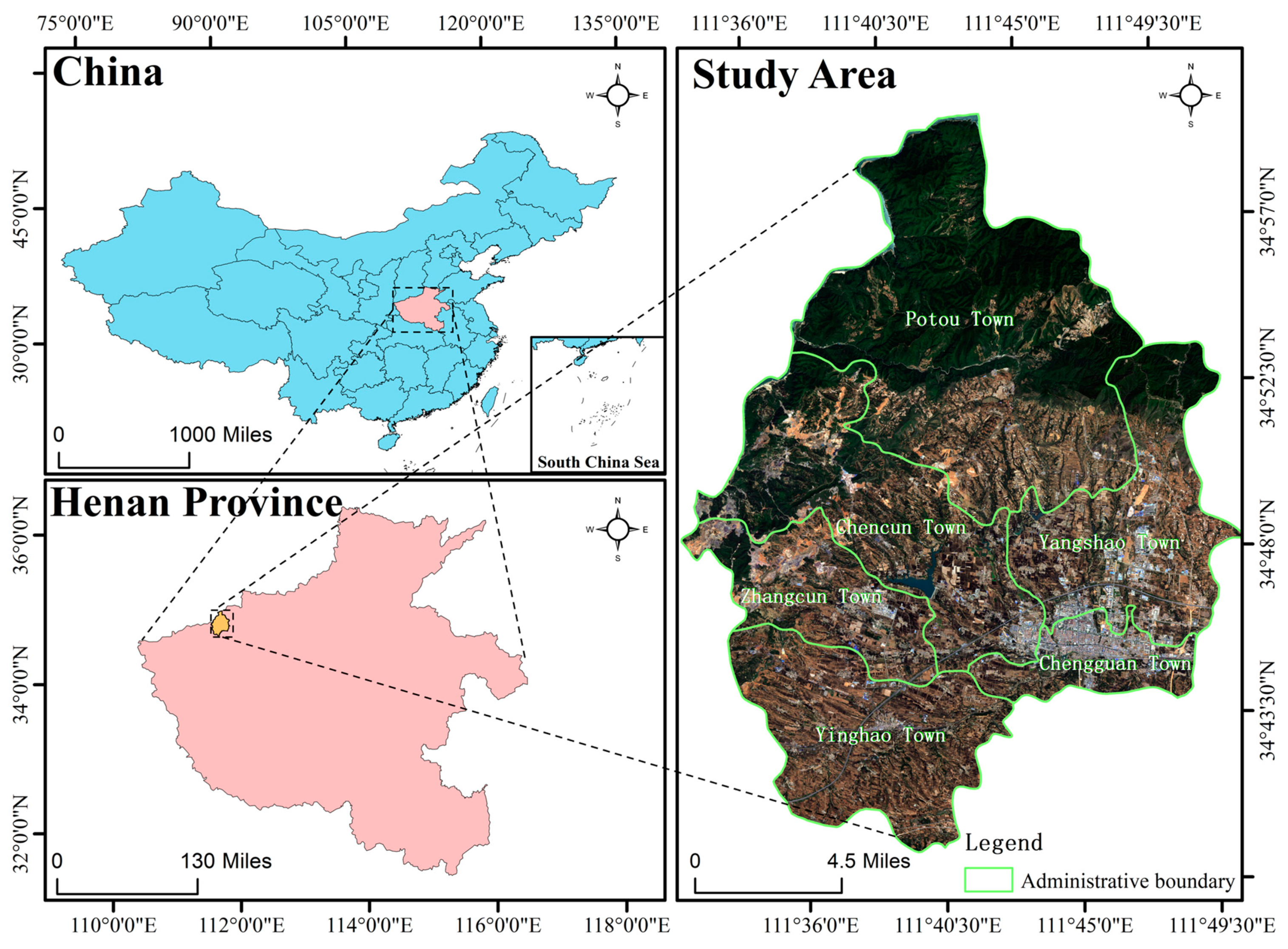
2.1.1. Study Area

Mianchi County is a typical agricultural county located in Sanmenxia City, Henan Province, China, whose geographical range covers (111°54′ E–111°85′ E, 34°67′ N–35°00′ N). The western part of Mianchi County was selected as the study area, covering 6 towns (Figure 1). In the north of the study area is a low mountainous area; the center is a trough basin, and the terrain is dominated by shallow hills. The region has a temperate continental monsoon climate, with an average annual temperature of 12.6 °C, annual precipitation of approximately 664.2 mm, and an average of 2362.2 h annual sunshine hours. Rain and heat occur at the same time, and seasonal changes are obvious. The farmland of the study area is approximately 235 square kilometers, accounting for 40.51% of the total area. The mainland types are brown soil and red clay, and a large amount of the farmland is distributed in the central basin and the northern hill area. The climatic conditions and soil conditions are suitable for the growth of food crops.

According to field investigations, the main crops grown in the study area are wheat, corn, and sweet potato, of which corn is biannual and the rest are annual. Most of the crops are sown around April, and the growth cycle is between April and September. In spring, corn, cotton, green beans, and sweet potatoes are planted. Corn is replanted in June and harvested around September, while wheat is sown at the end of September and the beginning of October and harvested at the end of May and beginning of June in the following year. The cycle of phenological changes for the main crops is shown in Figure 2.

2.1.2. Software

Remote-sensing data were processed and used to calculate the NDVI using ENVI software version 5.3.1. ArcGIS version 10.2 for desktop was used for image resampling, reclassifying, manual vectorization, NDVI calculation, random point generation, and extracting the difference value of the sample points.

2.1.3. Data Source

DEM data, land cover data, remote-sensing images, road network data, and administrative division data were used in this study. ALOS DEM data (12.5 m resolution) were obtained from the ASF search page of the NASA website [38], and GlobeLand V2020 land cover data were acquired from the official website of the National Center for Basic Geographic Information [39]. Road network data, including for railroads, highways, national roads, provincial roads, and urban primary, secondary, and tertiary roads, as well as administrative division data, including multi-year district and county administrative boundary data, were obtained from the Resource and Environmental Science Data Registration and Publication System (RESDPS) [40]. The remote-sensing images included GF-2 and GF-6 images, Landsat 8 images, and Google images, which were obtained from the Data Sharing Service System of GF Henan Center [41], the official website of the U.S. Geological Survey (USGS) [42], and the Google Earth page, respectively [43]. Of these, the GF data included multispectral bands (MSs) and panchromatic bands (PANs). The sensor types, temporal resolution, spatial resolution, and other parameters of the remote-sensing data are detailed in

Table 1. Parameters of remote-sensing data.

Feature	Landsat 8	GF-6	GF-2	Google Earth	ALOS
Data type	Remote-sensing data				DEM
Altitude (km)	705	645	631		692
Number of bands	11	PAN:8 MS:2	PAN:4 MS:1
Temporal resolution (d)	16	41	69		14
Spatial resolution (m)	30	PAN:2 MS:8	PAN:1 MS:4	0.6	12.5
Band/wavelength (μm)	B4/Red: 0.64–0.67	B3/Red: 0.63–0.69
	B5/NIR: 0.85–0.88	B4/NIR: 0.76–0.90
		MS: 0.45–0.90	MS: 0.45–0.90

. The administrative district data were used to extract the remote-sensing images, road network data, and land cover data from the study area. The land cover data were used to extract the extent of farmland and residential areas in the study area, and the DEM data were used to analyze the elevation and slope distribution of the abandoned farmland. The road network data were used to calculate the density of the road network in the study area to analyze the relationship between the distribution of abandoned farmland and the density of the road network. The residential area data were used to analyze the relationship between the distribution of abandoned farmland and the distance to residential areas, while the GF-6 and Landsat 8 images were used to calculate the NDVI and construct the NDVI time series dataset based on the STARFM. The GF-2, GF-6, and Google Earth images were used to obtain cultivated and abandoned farmland sampling points through visual interpretation.

2.1.4. Farmland Area Vectorization

The GlobeLand30 raster data were cropped and reclassified in ArcGIS to obtain the raster of the farmland region in the study area (Figure 3a), and the conversion tools in ArcGIS were used to convert the raster to a vector in order to obtain the vector boundary of the farmland area (Figure 3b). However, due to the fact that the spatial resolution of GlobeLand30 is coarser than the resolution of GF-6 data, many of the small features, as well as the feature boundaries, are biased and need to be adjusted manually. After the conversion process, a GF-6 image was used as the background for manual adjustment in ArcGIS (Figure 3c). The process is illustrated in Figure 3.

The base statistical data of the manual vectorization results are shown in

Table 2. Base statistics of farmland area vector.

Number of Polygons	Average Area	Minimum Area	Maximum Area	Median Area
193	1.24 km2	5.02 × 10−4 km2	191.75 km2	0.25 km2

.

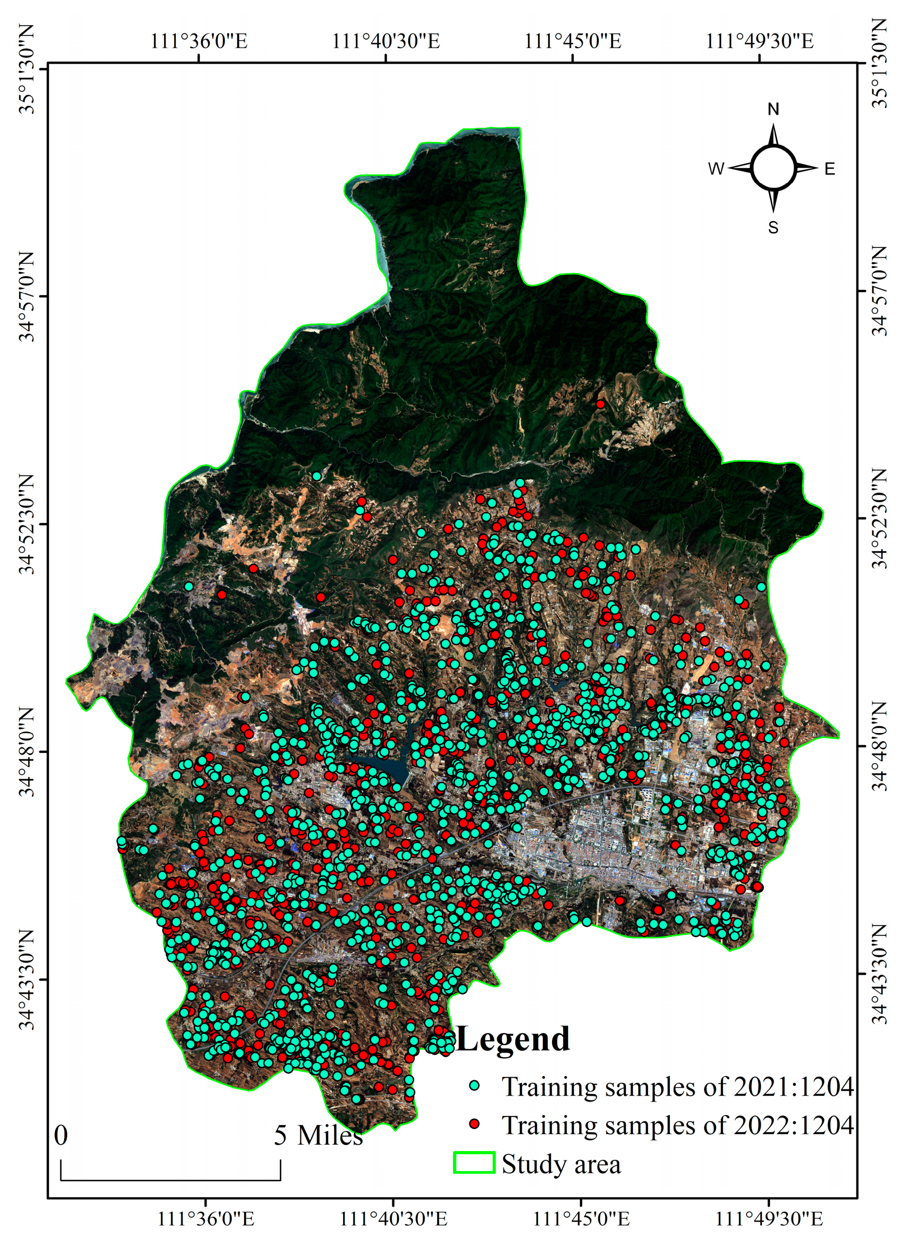
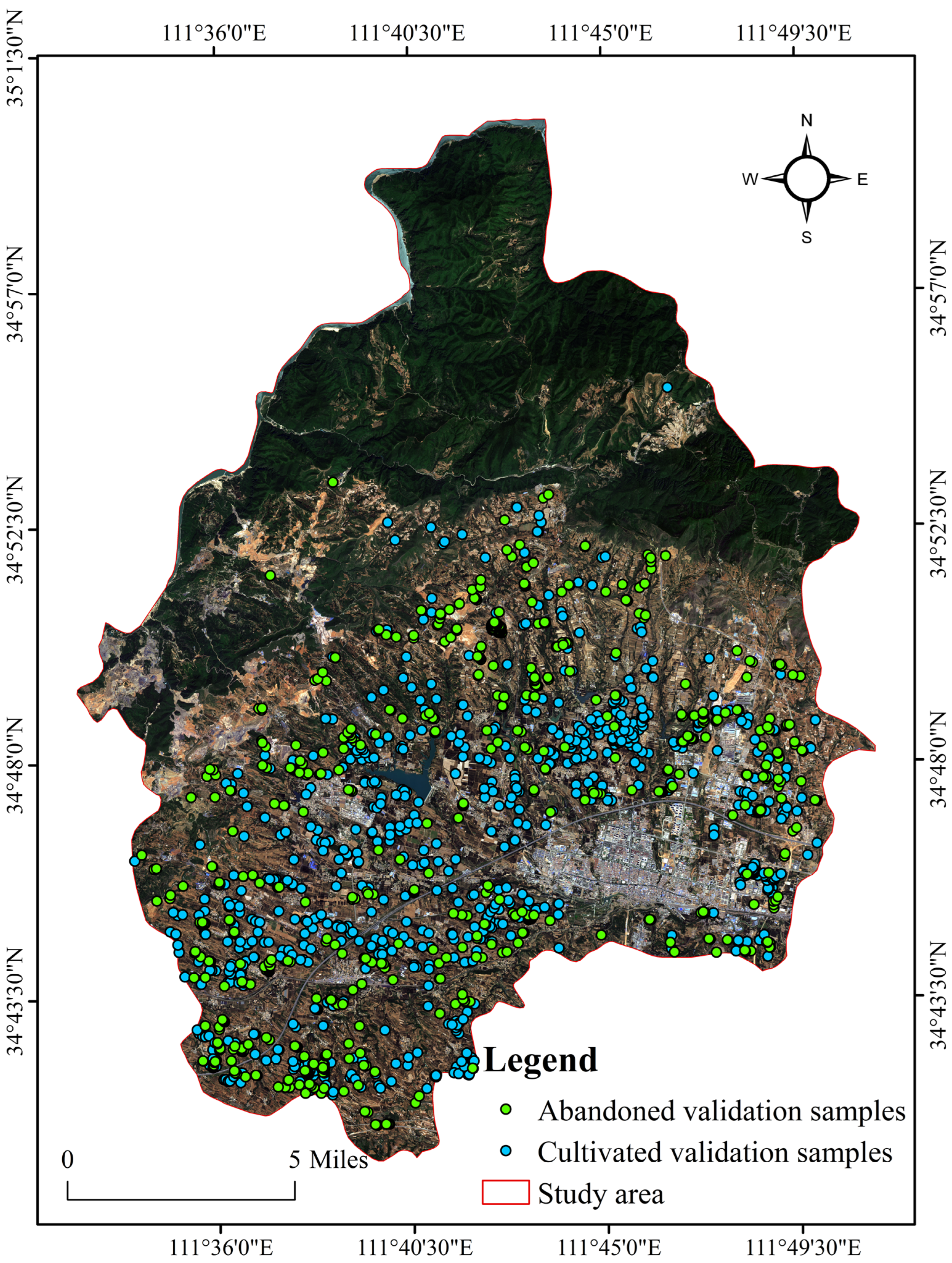
2.1.5. Sample Point Acquisition

ArcGIS software was used to generate random points within the vector boundaries of the farmland in the study area. These random points were visually interpreted based on GF images (including GF-2 and GF-6) and Google Earth images to obtain the samples with and without cropping activities in 2021 and 2022, respectively. The total number of sampling points was 6826, and 15% of the samples (1204 points) were randomly selected as training samples for the extraction of abandoned farmland data from 2021 and 2022, respectively. The distribution of the training sample points is shown in Figure 4.

2.2. Methods

Artificial crops have obvious cyclical changes in phenology due to human planting and harvesting activities, which can be subdivided into the “sowing stage”, “growing stage”, and “harvesting stage” according to the growth stage of the crops. We further define the time period when the crop grows from green to maturity as the growing stage (from the mid-sowing to mid-harvesting stage) and the rest as the non-growing stage. The NDVI is one of the important parameters reflecting crop growth and nutritional information. Due to human planting and harvesting activities, the NDVI of crops changes more obviously between the growing and non-growing stages than that of land with natural vegetation cover; that is, the difference in the NDVI of crops between the growing and non-growing stages will be greater, so we can extract abandoned farmland data based on this principle [20,24]. However, on the one hand, due to the effects of cloud and the low time resolution of the high-resolution data (GF-6 data), it is difficult to construct a time series dataset with cloud-free images that cover the growing stage and the non-growing stage of the main crops for the whole study area, resulting in missing data for some of the timestamps [44]. On the other hand, obtaining images during the early stage of the growing period results in less of a difference between the NDVI of the crops and the natural vegetation cover, making it difficult to differentiate between them. These problems all affect the construction of the NDVI time series dataset, which will have an effect on the precision of the extracted results.

Therefore, in this study, we selected remote-sensing images based on the phenological changes in the major crops in the study area. We also fused GF-6 and Landsat 8 data using STARFM and constructed a time series dataset by combining the GF-6 data and STARFM-fused data to ensure that the growing and non-growing stages of the major crops were covered by the less cloudy GF-6 resolution data and that the data from the growing period were not obtained during the early stage. The NDVI time series dataset was further divided into four time periods each year and ensured that these four time periods could cover both the growing and non-growing stages of the major crops. The difference in the NDVI values was calculated for each two adjacent time periods. The maximum value composite (MVC) process for the year was calculated to obtain the maximum NDVI difference for the neighboring periods in the year, which was taken as the annual NDVI difference. Then, visually interpreted sample points based on GF-2, GF-6, and Google Earth images were used to statistically obtain the threshold to segment the abandoned land. Finally, the two years of abandoned land data were overlain to determine the permanently abandoned farmland during these two years. The specific abandonment data extraction technology route is shown in Figure 5.

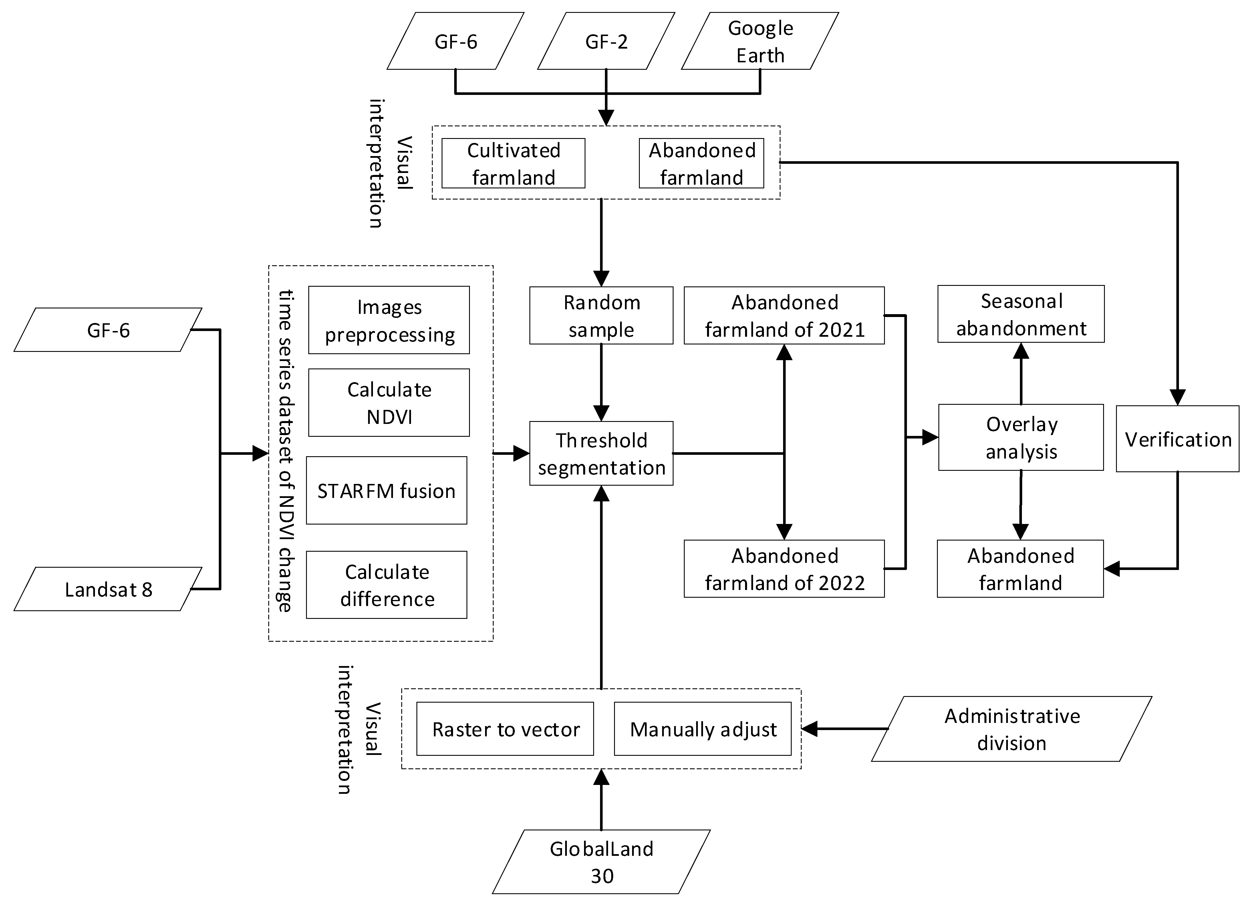
2.2.1. Data Processing

The DEM data and the land cover data were transformed into the same projection as the remote-sensing image (UTM-zone49). The slope and elevation data were calculated using the DEM data, and the farmland area and residential area vector data were converted from the land cover raster using ArcGIS. Then, the GF-2 image was used as the base map and combined with visual interpretation to manually adjust and supplement the vector boundaries of the farmland area and residential area. The Landsat 8 data were of an L2 level and had undergone radiometric calibration and atmospheric correction. The remaining preprocessing steps for the remote-sensing images were as follows:

• Radiometric calibration and atmospheric correction: GF images were processed through the radiometric calibration tool “Radiometric Calibration” and the atmospheric correction tool “FLAASH Atmospheric Correction” in ENVI;
• Resample: GF-6 and Landsat 8 images in the near-infrared band and red band needed to be resampled to a resolution of 2 m using the cubic convolution method;
• Image registration: GF images and Landsat 8 images needed to be registered based on the GF-6 image from 26 November 2022;
• Band math: NDVI was calculated using GF-6 and Landsat 8 images, as follows:

  $$NDVI=\frac{NIR-R}{NIR+R}$$

  (1)

  where NIR is the near-infrared band, and R is the red band of GF-6 or Landsat 8 images;
• STARFM spatial–temporal fusion: The NDVI computed from GF-6 and Landsat 8 images, obtained at a similar time, and the NDVI computed from a Landsat 8 image, obtained at another time without a GF-6 image covered, were selected to predict the GF-6 resolution-like (resolution of 2 m) NDVI.

2.2.2. STARFM

STARFM is a moving-window-based temporal and spatial resolution fusion algorithm that can not only be applied to the fusion of surface reflectance but can also be directly used for the fusion of NDVI and achieve good results [30,45].

Without considering geographic errors and the atmospheric correction error, the algorithm assumes that, under the condition that the land cover type and the systematic error do not change with time, the high-resolution surface reflectance image at time$t_k$ can be predicted using just a pair of surface reflectance images consisting of a high-resolution image. A coarse-resolution image at the known reference time $t_0$ and another coarse-resolution image at time $t_k$ can also be predicted. First, a moving window of size w is set up to capture the neighboring similar pixels, and the weighting function $W_{ij0}$ is determined by calculating the spectral difference $S_{ij0}$, temporal difference $T_{ij0}$, and spatial difference $D_{ij0}$ between a pair of high-resolution and coarse-resolution scenes at time $t_0$. Then, a prediction is made for a high-resolution image at time$t_k$ based on the medium- and low-resolution image at time $t_k$. The calculation method is as follows:

$$G\left(X_{w/2},Y_{w/2},T_k\right)={\displaystyle \sum }_{i=1}^w{\displaystyle \sum }_{j=1}^w{\displaystyle \sum }_{k=1}^k{W}_{ijk}\times \left(L\left(X_i,Y_j,T_k\right)+G\left(X_i,Y_j,T_0\right)-L\left(X_i,Y_j,T_0\right)\right)$$

(2)

$$S_{ij0}=\left|G\left(X_i,Y_j,T_0\right)-L\left(X_i,Y_j,T_0\right)\right|$$

(3)

$$T_{ij0}=\left|G\left(X_i,Y_j,T_0\right)-L\left(X_i,Y_j,T_k\right)\right|$$

(4)

$$D_{ij0}=1+\sqrt{{\left(X_{w/2}-X_i\right)}^2+{\left(Y_{w/2}-Y_j\right)}^2}/A$$

(5)

$$W_{ij0}=S_{ij0}\times T_{ij0}\times D_{ij0}$$

(6)

where G and L denote the high-resolution image and coarse-resolution image, respectively, $X_i$, $Y_i$ denote homogeneous image elements, w denotes the moving window size, and A is a constant.

2.2.3. NDVI Difference Calculation

The growth cycle of crops can be divided into the “sowing stage”, “growing stage”, and “harvesting stage”, and the NDVI of crops between the growing and non-growing stages are more obvious than those of natural vegetation due to anthropogenic sowing and harvesting activities. In this study, the abandoned farmland data were extracted according to this principle. Therefore, we required a time series dataset that could cover the growing and non-growing stages of major crops in the study area and quantify the NDVI changes through the difference in the NDVI values between the growing and non-growing stages.

Firstly, the year was divided into four time periods (January–March, April–June, July–October, and November–December) according to the growing and non-growing period patterns of the crops in this study area (Figure 1). These four periods should cover the growing and non-growing stages of the crops and, further, should ensure that each time period was covered by the NDVI data. However, due to the influence of the low temporal resolution of the data, as well as cloudy weather, the use of GF-6 data as a single data source often fails to cover the growing and non-growing stages of the major crops in this area. As a consequence, in this study, STARFM was utilized to fuse the GF-6 and Landsat 8 data to obtain the GF-6 resolution-like NDVI data, which were combined with the GF-6 data to jointly construct the NDVI time series dataset. Then, the NDVI of adjacent time periods were differenced, and the absolute values were taken. If there was multiple NDVI data coverage in a certain time period, an MVC was taken after separate calculations, and the result was used to measure the NDVI changes in the two adjacent time periods. Lastly, the three NDVI differences between the four time periods were composited into the NDVI difference of the year based on the MVC to measure the NDVI changes in that year. The calculation process was as follows:

$$NDVI differenc{e}_{season}=max\{NDVI\left(i,m\right)-NDVI\left(j,n\right))$$

(7)

$$NDVI differenc{e}_{year}=max\left\{NDVI differenc{e}_{season}\right\}$$

(8)

where $NDVI differenc{e}_{season}$ is the NDVI difference in one season, $NDVI differenc{e}_{year}$ is the NDVI difference in one year, i, and j represent the ith and jth adjacent time periods, and m and n represent the number of NDVI data in ith and jth time period.

2.2.4. Abandoned Farmland Data Extraction

In this study, abandoned farmland data were extracted based on the differences in the NDVI changes between the growing and non-growing stages of the crops and natural vegetation. First, we visually interpreted the sampling points with GF-2, GF-6, and Google Earth images and defined the points with no crop growth in a year as abandoned points. Then, we inputted the annual NDVI difference value to the sampling points in ArcGIS and statistically obtained the range of values of the annual NDVI difference for all sampling points. After this, we divided the range into ten intervals and statistically analyzed the proportion of abandoned points to all points in each interval. The segmentation threshold was determined by the interval where the inflection point of the curve of the change in its proportion was located. Then, the data regarding cultivated and abandoned land in each year were extracted by the threshold segmentation; the parts with a value less than the threshold were considered abandoned land, while the rest were not. Finally, the area of abandoned land for each year was overlain to obtain the total area of abandoned farmland for these two years.

2.2.5. Accuracy Assessment

To verify the accuracy of the abandoned farmland extraction results, random points located on the farmland in the study area were generated using ArcGIS software. Then, high-resolution remote-sensing images (GF-2, GF-6, and Google Earth images) were used to determine whether each random point location was abandoned or not using visual interpretation in order of the image date. A point with no crop planted in the imagery for each date represented abandonment; otherwise, it did not. The obtained validation sampling points were overlain with the extraction results. The different types of validation sampling points (abandoned points and cultivated points), falling inside and outside the abandoned farmland extraction results, were counted separately in order to construct the confusion matrix. Then, the overall accuracy and Kappa coefficient were calculated to evaluate the extraction results based on the confusion matrix, which was then used to measure the precision and consistency of the extraction results. The overall accuracy and Kappa coefficient were calculated as follows:

$$Overall Accuracy=P_0=\frac{TP+TN}{TP+FP+TN+FN}$$

(9)

$$P_e=\frac{\left(TP+FN\right)\ast \left(TP+FP\right)+\left(FN+TN\right)\ast \left(FP+TN\right)}{{\left(TP+FP+FN+TN\right)}^2}$$

(10)

$$Kappa coefficient=\frac{P_0-P_e}{1-P_e}$$

(11)

where TP represents true positive, TN represents true negative, FP represents false positive, and FN represents false negative.

In order to verify that the STARFM-fused dataset could effectively improve the accuracy of the extracted abandoned farmland data using an NDVI time series analysis, this study additionally extracted the results using only GF-6 and Landsat 8 data, which were then used for a comparison of the accuracy of the results. In addition, Support Vector Machine (SVM), a supervised classification algorithm based on statistical learning theory, was utilized. In this approach, a hyperplane between different categories was obtained based on the edge sample and was used for sample classification and abandoned farmland data extraction using a multidimensional NDVI time series dataset classification, obtaining good results. The SVM classified the data from the NDVI in different dimensions of the dataset, ignoring the changes in the NDVI between two adjacent time periods. Therefore, the SVM was additionally used for abandoned farmland data extraction based on the STARFM-fused NDVI time series dataset to verify the accuracy of the results based on the NDVI time series analysis.

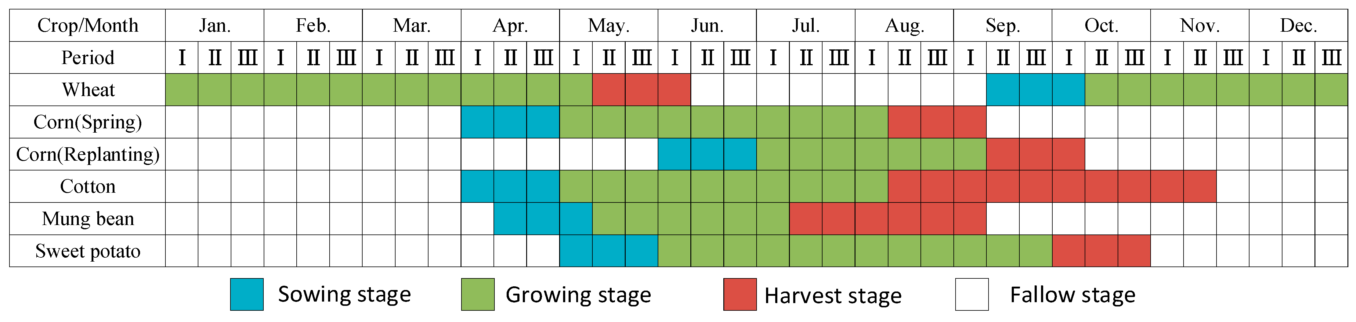
2.2.6. Farmland Abandonment Feature Analysis

Farmland abandonment is affected by various factors, which can be divided into natural and human factors. Natural factors include the topography, climate, precipitation, and distance from forests, while human factors include the distance from residential areas, labor loss, and transportation accessibility [21,46,47]. In this study, two natural factors, elevation and slope, and two human factors, distance from settlement and road network density, were selected to analyze the influence of farmland abandonment. Elevation and slope were calculated based on the DEM. The elevation was divided into four grades according to intervals of 200 m, and the slope was divided into six grades according to intervals of 5°. For the distance from the residential area, multi-ring buffers at 200 m intervals were constructed according to the boundary of the residential area vector. For the density of the road network, the density was calculated according to the road network vector line elements and was graded according to natural breaks.

After obtaining the grades for the different influence factors, the results of the extraction of influence factors and abandoned farmland were overlain and analyzed to obtain the number of abandoned farmland grid points in each grade for each influence factor. The ratio of abandoned farmland grid points to the total number of points in each grade was calculated, which was then used to measure the magnitude of the effect of the factor on farmland abandonment. Then, the abandonment rate was calculated based on the proportion of abandoned grid points to the total number of grid points in the region. The calculation methods for the magnitude and abandonment rate are as follows:

$$Magnitude=\frac{A_i}{A_{total}}$$

(12)

$$Abandonment rate=\frac{A_i}{F_{total}}$$

(13)

where $A_i$ is the number of abandoned grid points in the region or different grades of influence factors, $A_{total}$ is the number of all abandoned grid points, and $F_{total}$ is the number of all farmland grid points.

3. Results

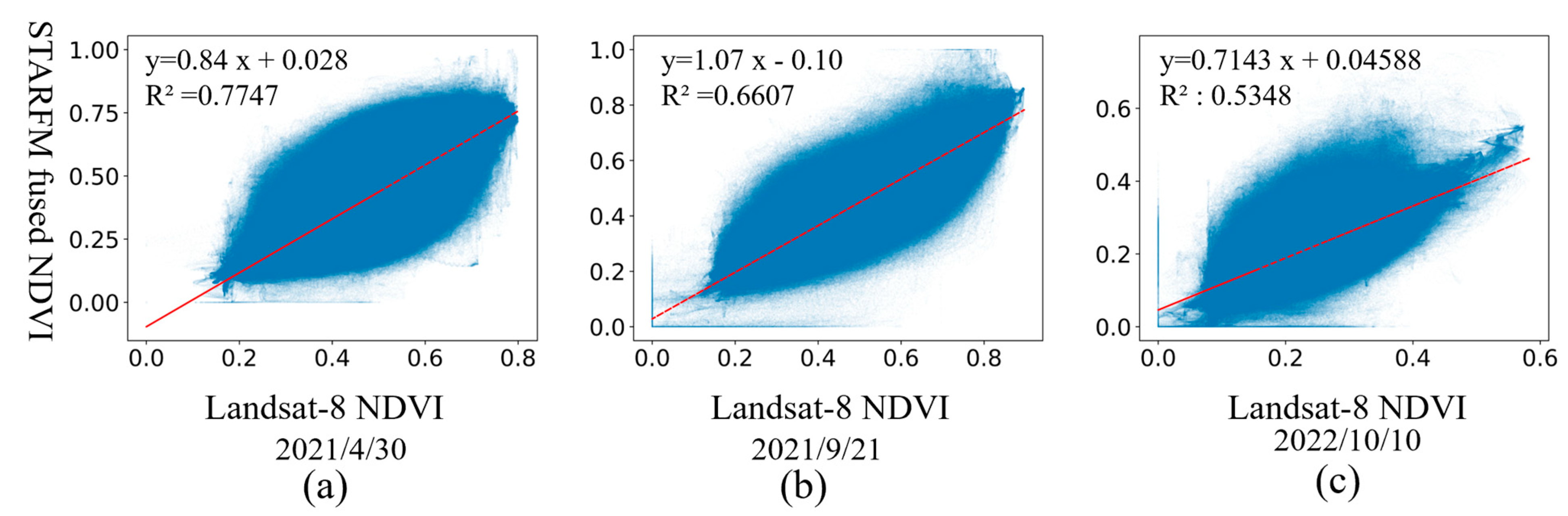
3.1. NDVI Temporal–Spatial Fusion

In this study, pairs of GF-6 and Landsat 8 NDVIs from similar times on 26 November 2021, 11 June 2021, and 26 November 2022, and Landsat8 NDVIs from 21 September 2021, 30 April 2021, and 10 October 2022 were selected to fuse the GF-6 resolution-like (resolution of 2 m) NDVI on 30 April 2021, 21 September 2021, and 10 October 2022. The correspondence between the base NDVI and the fused NDVI is shown in

Table 3. Dates of GF-6 NDVI, Landsat 8 NDVI, and corresponding STARFM-fused NDVI.

Date of GF-6 NDVI	Date of Landsat 8 NDVI	Date of STARFM-Fused NDVI
11 June 2021	14 June 2021	30 April 2021
26 November 2021	26 November 2021	21 September 2021
26 November 2022	26 November 2022	10 October 2022

.

The base NDVI and fused NDVI results are shown in Figure 6, and the correlation between the Landsat 8 NDVI and STARFM-fused NDVI is shown in Figure 7.

3.2. NDVI Difference Calculation

According to the cycle pattern of characteristics of the crop phenology in the study area (Figure 2), the GF-6 NDVI in March and November 2021 and February, May, July, and November 2022, and the fused GF-6 resolution-like NDVI (resolution of 2 m) in April and September 2021 and October 2022 from STARFM were selected to construct the NDVI time series dataset in 2021 and 2022. This ensured that a high-resolution NDVI covered the growing and non-growing stages and growth changes of the main crops in the study area. The selected dates for the GF-6 NDVI and fused NDVI are shown in

Table 4. Types and dates of NDVI used to construct time series datasets.

Year of Time Series Dataset	Date of GF-6	Date of STARFM-Fused Data
2021	25 March	30 April
	26 November	21 September
2022	24 February
	5 May	10 October
	1 July
	26 November

.

The difference in the NDVI for each of the two adjacent stages was calculated separately, and the absolute value was taken to measure the degree of drastic changes in the NDVI between the two stages. Then, the maximum value of each NDVI difference was composited for 2021 and 2022 as the degree of drastic change in the NDVI for 2021 (Figure 8a) and 2022 (Figure 8b), respectively.

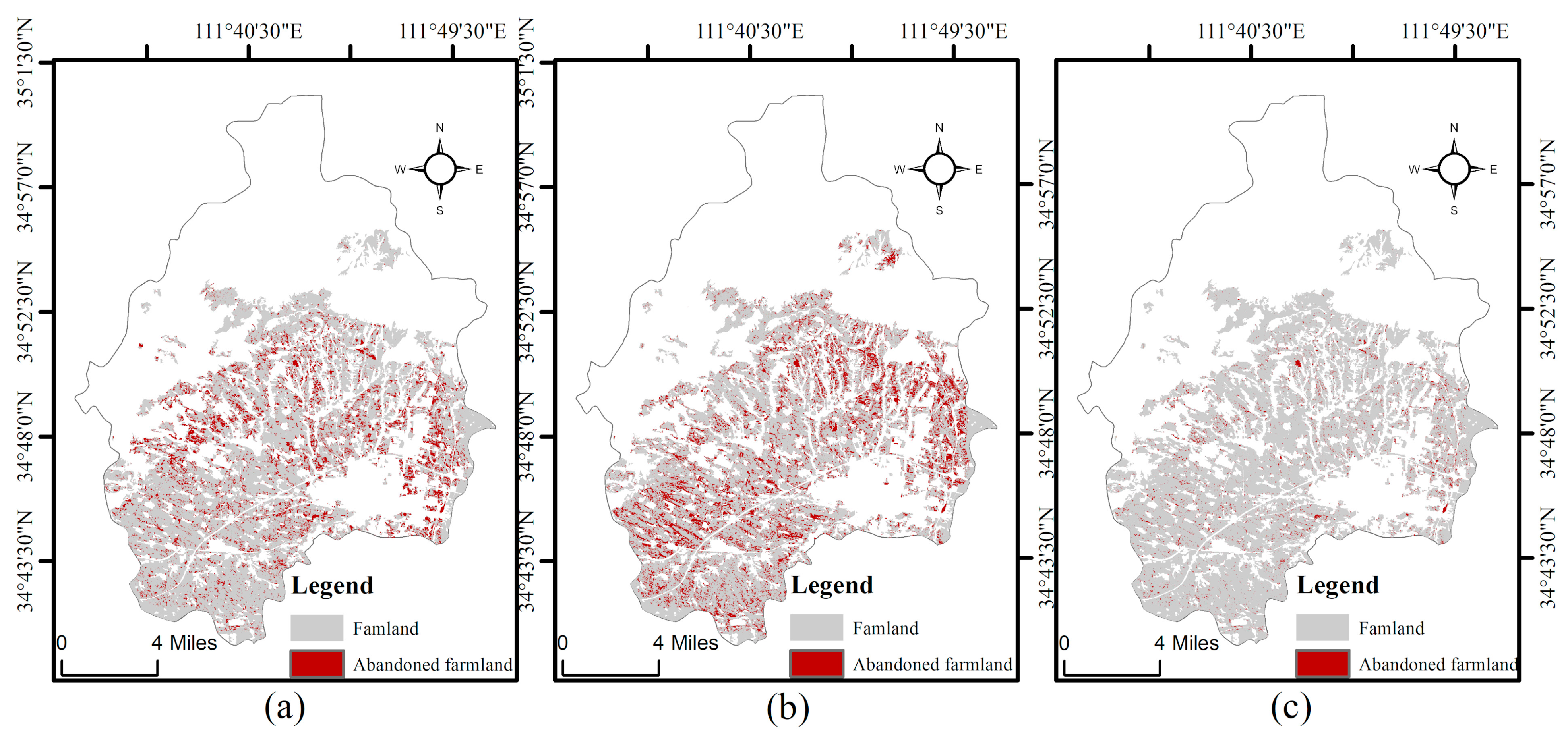
3.3. Abandoned Farmland Data Extraction

First, the NDVI values were equally divided into ten intervals and then extracted to the sampling points using ArcGIS software. Then, the proportion of abandoned sampling points to all points in each interval was calculated separately, and the thresholds were determined by the inflection point of the proportional change curve. The proportional change curves and their inflection points for 2021 and 2022 are shown in Figure 9a,b. The inflection point was located in the range of [0.21, 0.29) in 2021 and [0.14, 0.21) in 2022.

The threshold was set to 0.29 in 2021 and 0.21 in 2022, with abandoned land showing a value less than the threshold and cultivated farmland exhibiting a value greater than the threshold during the year. The two-year abandoned farmland area data were overlain to distinguish between permanent abandonment and seasonal abandonment.

The abandoned farmland for 2021 is shown in Figure 10a, and that of 2022 is shown in Figure 10b. The area of permanently abandoned farmland was obtained by overlaying the extraction results for 2021 and 2022, as shown in Figure 10c.

3.4. Extraction Result Accuracy and Comparison

Based on the visual interpretation of Google Earth, GF-2, and GF-6 images, a total of 1476 sampling points for validation were obtained for the period 2021–2022. The sampling points were overlain with the abandonment of farmland extraction results (Figure 11), and the extraction results are shown separately in Figure 12b. After counting the extraction results and the true values of the validation set, the overall accuracy of the extraction was calculated as 93.43% with a Kappa coefficient of 0.87.

Additionally, based on the method of this study, the results of the abandoned farmland data extraction using only the GF-6 dataset are shown in Figure 12a. The results using an NDVI time series analysis based on only Landsat data are shown in Figure 12c, and the results using an SVM for time series analysis based on the STARFM-fused data are shown in Figure 12d.

The accuracy of the different methods based on different data is shown in

Table 5. Overall accuracy and Kappa coefficient of results using different extraction methods with different data.

Analysis Method	Dataset	Overall Accuracy	Kappa Coefficient
NDVI difference	GF-6 dataset	78.93%	0.58
NDVI difference	Fusion dataset 1	93.43%	0.87
NDVI difference	Landsat dataset	64.91%	0.30
SVM	Fusion dataset	83.94%	0.68

¹ NDVI time series dataset fused based on GF-6 and Landsat 8 data.

.

3.5. Analysis of the Spatial Distribution of Abandoned Farmland

3.5.1. Overall Distribution of Abandoned Farmland in the Study Area

The total farmland in the study area is approximately 235 square kilometers, and the results of the abandoned land data extraction, shown in Figure 12a, indicate that the area of abandoned land in the study area is approximately 12.73 square kilometers, with an abandonment rate of 5.42%. According to the results of this study, the overall spatial distribution of abandoned land was mainly distributed in the central and western parts of the study area. For the kernel density analysis of the abandoned land extraction results, we selected three high-density areas as examples to show the distribution of features around these areas, as shown in Figure 13. As can be observed, the high-density areas are mostly located in residential areas and areas where roads intersect, probably due to the influence of road density, automobile exhausts, and building construction.

3.5.2. Feature Analysis of Abandoned Farmland

The slopes in the study area were divided into six slope ranges: 0–5°, 5–10°, 10–15°, 15–20°, 20–25°, and 25° or more, at fixed intervals of 5°. The area of land abandonment patches within each slope range and the proportion in the total study area were counted. The proportion of abandoned farmland to all farmland and the abandonment rates at different intervals are shown in Figure 14a.

The DEM in the study area was divided into four categories, with 400 m, 600 m, and 800 m as the breakpoints. The area of abandoned land patches within the elevation range of each category and the proportion in the total study area were counted. The proportion of abandoned farmland to all farmland and the abandonment rates at different intervals are shown in Figure 14b.

From the abandonment data extraction results and the kernel density analysis, it can be generally observed that the abandoned farmland in the study area is concentrated around residential areas. Thus, the distribution of abandoned farmland may be related to the distance from residential areas as well as the density of the road network.

A line density analysis of the road network in the study area was carried out. The road network density was divided into five categories—extremely low, low, medium, high, and extremely high—according to the natural breaks. The area of abandoned farmland patches in each category and the proportion of abandoned farmland in the total farmland area was calculated, as shown in Figure 14c.

Multi-ring buffers were established at an interval of 200 m from the vector boundary of the residential areas, and the cultivated areas were divided into areas 200 m, 200–400 m, 400–600 m, 600–800 m, and 800 m away from the residential areas. The area of abandoned land patches in different buffer zones and its proportion to the total area of abandoned land was calculated separately. The proportion of abandoned farmland to all farmland and the abandonment rates at different intervals are shown in Figure 14d.

The area of total farmland, the area of farmland under cultivation, the area of abandoned farmland, and the abandonment rate of farmland in different ranges with different influencing factors, including elevation, slope, density of the road network, and distance from residential areas, are shown in

Table 6. Farmland area and abandonment rate in different ranges for different features.

Feature	Range	Farmland Area/km2	Cultivation Area/km2	Abandonment Area/km2	Abandonment Rate/%
Elevation	<400 m	0.42	0.41	0.01	2.77
	400–600 m	122.66	115.75	6.91	5.63
	600–800 m	99.75	94.14	5.61	5.62
	>800 m	9.58	9.37	0.21	2.15
Slope	0–5°	98.81	92.45	6.36	6.44
	5–10°	82.55	77.81	4.74	5.74
	10–15°	36.71	35.37	1.34	3.65
	15–20°	11.66	11.41	0.25	2.14
	20–25°	2.26	2.23	0.03	1.31
	>25°	0.42	0.39	0.03	7.04
Distance to residential area	0–200 m	96.94	90.77	6.17	6.36
	200–400 m	71.82	67.82	4.00	5.57
	400–600 m	31.94	30.21	1.73	5.42
	600–800 m	12.26	11.66	0.60	4.89
	>800 m	19.45	19.21	0.24	1.23
Road density	Extremely low	112.73	108.17	4.56	4.05
	Low	79.85	74.91	4.94	6.19
	Medium	33.04	30.74	2.30	6.96
	High	5.57	4.92	0.65	11.67
	Extremely high	1.22	0.93	0.29	23.77

.

4. Discussion

4.1. Abandoned Farmland Data Extraction

The high spatial resolution of GF-6 images can effectively improve the accuracy of the results, but it is difficult to construct a continuous and widely covered time series dataset due to the low temporal resolution and the influence of weather. To address this problem, this study fused GF-6 and Landsat 8 data based on STARFM to construct the NDVI time series dataset and then extracted abandoned farmland data based on the differences in the NDVI cycle changes between natural vegetation and planted crops. The overall accuracy and Kappa coefficient of the extraction results were significantly improved compared with those obtained by using GF-6 data or Landsat 8 data alone. In addition, for the time series analysis based on the SVM, the overall accuracy and Kappa coefficient using the fused dataset were also improved, which proved that the fused dataset could, indeed, improve the accuracy of the abandoned cropland data extraction results. The overall accuracy and Kappa coefficient of the extraction results of this study are also higher than those obtained from the SVM-based analysis based on the fused dataset. Using the SVM for analysis also enables the extraction of abandoned farmland data, but it is easier to misidentify cultivated land as abandoned land, resulting in the expansion of the scope of the abandoned land. Compared with the results obtained by studies using SVM, the results of this study are able to better distinguish between abandoned land and cultivated land, with higher precision and consistency.

4.2. Limitations and Prospects

In this study, the fusion of GF-6 and Landsat 8 images using the STARFM algorithm solves the problem of accuracy degradation caused by the low temporal resolution in constructing the time series dataset, which requires a low amount of data. However, since the predictive accuracy of the STARFM algorithm decreases as the difference between the prediction date and the base date increases [48], it may be difficult to generalize when only GF-6 and Landsat 8 data are used. Additionally, while an NDVI time series analysis is a commonly used method, it is difficult to capture vegetation features that are insensitive to the linear relationship between NIR and R bands using this approach, resulting in decreased accuracy [49]. In subsequent studies, we can continue to improve or try other spatial–temporal fusion strategies, combine more types of remote-sensing data (e.g., GF-1, GF-4, and GF-6 grouped data), and combine multiple vegetation indices for time series analysis in order to continue to improve the accuracy of the results.

4.3. Abandoned Farmland Feature Analysis

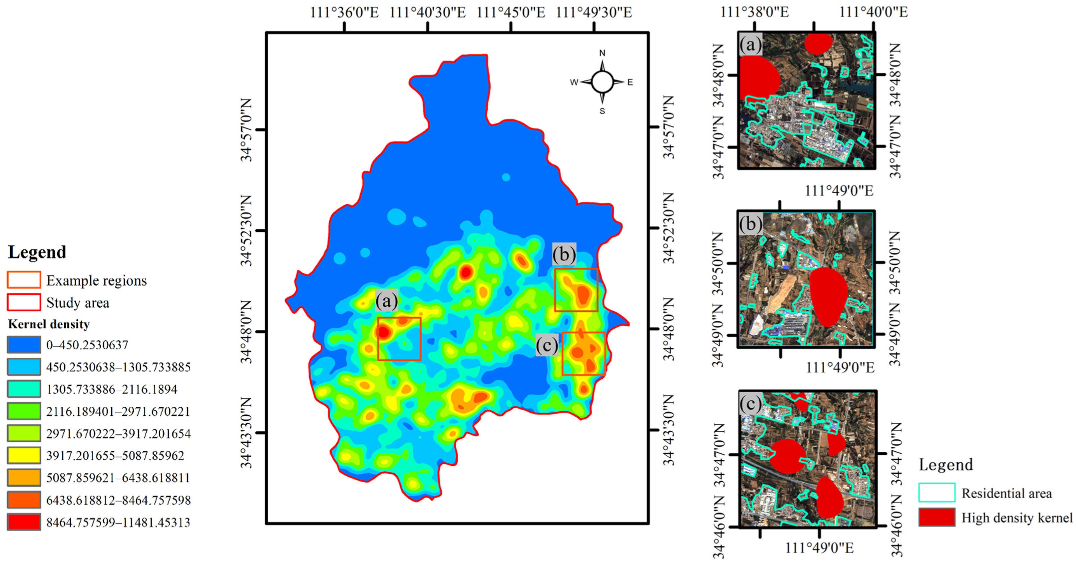
• The total area of abandoned farmland in the study area was approximately 12.73 square kilometers, and the overall abandonment rate was 5.43%. The kernel density analysis of the abandoned farmland showed that there were five highest-level density kernels distributed in the south, southeast, southwest, and central parts of the study area; these were generally distributed around the edge of the residential area in a ring shape;
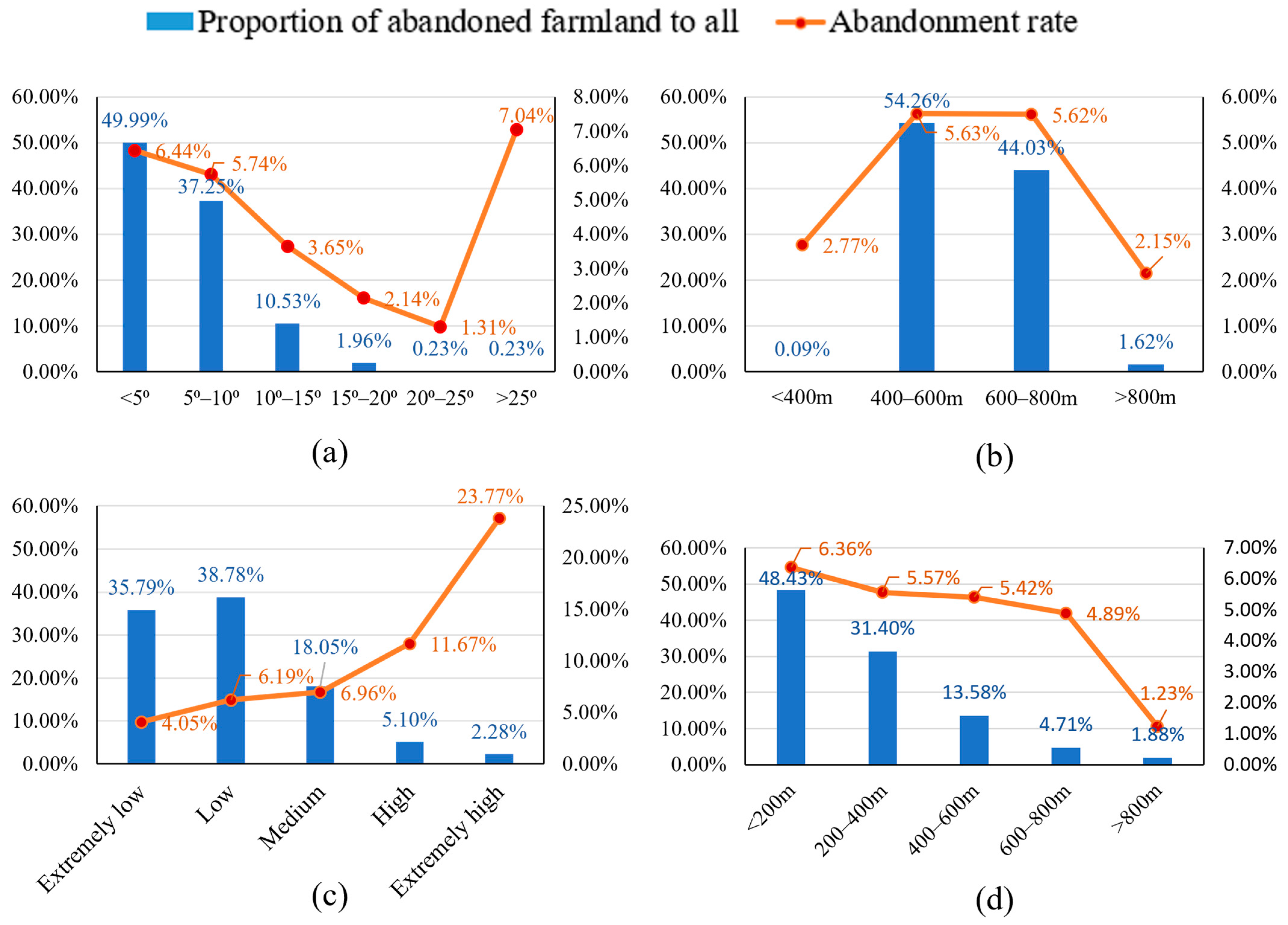
• In the study area, the abandoned farmland and areas with high abandonment rates were mainly distributed in the elevation range of 400–800 m and the slope range of 0–10°. Although the abandonment rate in the areas with a high slope range (>25°) was significantly higher than the overall abandonment rate, the distribution of cultivated land in this area was very small. Therefore, the cultivated land and abandoned farmland, in general, were mainly distributed in the areas of low slope and low elevation. On the one hand, elevation and slope affect temperature, soil and water conservation, and light. On the other hand, they limit accessibility and large-scale mechanized agriculture; therefore, locations for farming are more likely to be chosen in areas with flat terrain and lower elevations;
• The distribution of abandoned farmland in the study area varies with the density of the road network. The area of abandoned land increases with the decrease in the road network density, but the abandonment rate decreases with the decrease in the road network density. Road network density directly affects the accessibility of transportation, and areas with high road network density are more suitable for large-scale mechanized agriculture and the transportation of crops and agricultural tools. At the same time, a highly dense road network also means the abandonment or even the occupation of the surrounding farmland;
• The area of abandoned farmland and the abandonment rate both increase with decreasing distance from residential areas. The distance from settlements is related to the expansion of construction land, and urbanization may lead to the abandonment of farmland near residential areas or even lead to a change in the land use type, resulting in an increase in the farmland abandonment rate.

5. Conclusions

In this study, we constructed an NDVI time series dataset based on the fusion of GF-6 and Landsat 8 images using STARFM. We combined this dataset with the phenological changes in the major crops in the study area and extracted data related to permanently abandoned farmland for the period of 2021–2022 based on the threshold segmentation of the annual NDVI change and overlay analysis. We verified the accuracy of the extraction results using visual interpretation. Based on the results of the abandoned farmland data extraction, the following conclusions were drawn regarding the features of abandoned farmland in different elevation ranges, slope ranges, distances from residential areas, and road network densities:

• By fusing GF-6 and Landsat 8 images using STARFM to construct a dataset for time series analysis, the accuracy of the results can be effectively improved compared with the use of GF-6 data alone. This study is based on the difference in the NDVI values at different stages of the crop growth cycle, which is more effective for distinguishing between abandoned land and cultivated land. The accuracy of the results is higher than that obtained using SVM. The method is feasible, and the results are valid and reliable;
• On the basis of the extraction results, the features of abandoned farmland in the study area were analyzed. The results show that most of the farmland in Mianchi County is located in areas of terrain suitable for farming and that abandoned cultivated land is not as affected by elevation and slope as it is by the density of the road network and proximity to residential areas. Abandonment rates tend to be higher in areas with a high road density and close to residential areas. These results may help in the management of cropland abandonment and the regulation of farmland.

Due to the data collection and fusion methods used, this study has some limitations:

• Although the GF-6 data are of high resolution, they have fewer bands than other sensor-type data. Consequently, these data can only be analyzed by calculating several VIs for analysis, and only the NDVI was used in this study, which is a limitation for abandoned farmland data extraction;
• When high-resolution NDVI fusion is based on STARFM, the fused value of regions with abrupt NDVI changes is larger than the real value. The fusion accuracy decreases with the increase in the difference between the base date and the prediction date, which has an impact on the accuracy of the extraction results for abandoned farmland. Moreover, it is difficult to generalize the results to regions where cloudy and rainy weather persist for a long period of time.

References

1. Huang, Y.; Li, F.; Xie, H. A Scientometrics Review on Farmland Abandonment Research. Land 2020, 9, 263. [Google Scholar] [CrossRef]
2. Weissgerber, M.; Chanteloup, L.; Bonis, A. Perceptions of Vegetation Succession Following Agricultural Abandonment in the Massif Central Region (France). Landsc. Urban Plan. 2023, 234, 104717. [Google Scholar] [CrossRef]
3. Chen, R.; Ye, C.; Cai, Y.; Xing, X.; Chen, Q. The Impact of Rural Out-Migration on Land Use Transition in China: Past, Present and Trend. Land use policy 2014, 40, 101–110. [Google Scholar] [CrossRef]
4. Xu, D.; Deng, X.; Guo, S.; Liu, S. Labor Migration and Farmland Abandonment in Rural China: Empirical Results and Policy Implications. J. Environ. Manag. 2019, 232, 738–750. [Google Scholar] [CrossRef] [PubMed]
5. Chaudhary, S.; Wang, Y.; Dixit, A.M.; Khanal, N.R.; Xu, P.; Fu, B.; Yan, K.; Liu, Q.; Lu, Y.; Li, M. A Synopsis of Farmland Abandonment and Its Driving Factors in Nepal. Land 2020, 9, 84. [Google Scholar] [CrossRef]
6. Estel, S.; Kuemmerle, T.; Alcántara, C.; Levers, C.; Prishchepov, A.; Hostert, P. Mapping Farmland Abandonment and Recultivation across Europe Using MODIS NDVI Time Series. Remote Sens. Environ. 2015, 163, 312–325. [Google Scholar] [CrossRef]
7. Li, L.; Pan, Y.; Zheng, R.; Liu, X. Understanding the Spatiotemporal Patterns of Seasonal, Annual, and Consecutive Farmland Abandonment in China with Time-Series MODIS Images during the Period 2005–2019. Land Degrad. Dev. 2022, 33, 1608–1625. [Google Scholar] [CrossRef]
8. Qiu, Y.; Cao, G. The Heterogeneous Effects of Multilevel Location on Farmland Abandonment: A Village-Level Case Study in Tai’an City, China. Land 2022, 11, 1233. [Google Scholar] [CrossRef]
9. Mianchi County People’s Government’s Notice on Further Strengthening and Standardizing the Post-Project Management and Care of Land Improvement Projects. Available online: https://www.mianchi.gov.cn/23341/615785472/1428432.html (accessed on 16 February 2024).
10. Smaliychuk, A.; Mueller, D.; Prishchepov, A.V.; Levers, C.; Kruhlov, I.; Kuemmerle, T. Recultivation of Abandoned Agricultural Lands in Ukraine: Patterns and Drivers. Glob. Environ. Chang.-Hum. Policy Dimens. 2016, 38, 70–81. [Google Scholar] [CrossRef]
11. Keenleyside, C.; Tucker, G.; McConville, A. Farmland Abandonment in the EU: An Assessment of Trends and Prospects; Institute for European Environmental Policy: London, UK, 2010; pp. 1–98. [Google Scholar]
12. Xiao, G.; Zhu, X.; Hou, C.; Xia, X. Extraction and Analysis of Abandoned Farmland: A Case Study of Qingyun and Wudi Counties in Shandong Province. J. Geogr. Sci. 2019, 29, 581–597. [Google Scholar] [CrossRef]
13. Khanal, N.R.; Watanabe, T. Abandonment of Agricultural Land and Its Consequences. Mred 2006, 26, 32–40. [Google Scholar] [CrossRef]
14. Yin, H.; Prishchepov, A.V.; Kuemmerle, T.; Bleyhl, B.; Buchner, J.; Radeloff, V.C. Mapping Agricultural Land Abandonment from Spatial and Temporal Segmentation of Landsat Time Series. Remote Sens. Environ. 2018, 210, 12–24. [Google Scholar] [CrossRef]
15. Wu, J.; Jin, S.; Zhu, G.; Guo, J. Monitoring of Cropland Abandonment Based on Long Time Series Remote Sensing Data: A Case Study of Fujian Province, China. Agronomy 2023, 13, 1585. [Google Scholar] [CrossRef]
16. Alcantara, C.; Kuemmerle, T.; Baumann, M.; Bragina, E.V.; Griffiths, P.; Hostert, P.; Knorn, J.; Mueller, D.; Prishchepov, A.V.; Schierhorn, F.; et al. Mapping the Extent of Abandoned Farmland in Central and Eastern Europe Using MODIS Time Series Satellite Data. Environ. Res. Lett. 2013, 8, 035035. [Google Scholar] [CrossRef]
17. Liu, B.; Song, W.; Sun, Q. Status, Trend, and Prospect of Global Farmland Abandonment Research: A Bibliometric Analysis. IJERPH 2022, 19, 16007. [Google Scholar] [CrossRef]
18. Wei, Z.; Gu, X.; Sun, Q.; Hu, X.; Gao, Y. Analysis of the Spatial and Temporal Pattern of Changes in Abandoned Farmland Based on Long Time Series of Remote Sensing Data. Remote Sens. 2021, 13, 2549. [Google Scholar] [CrossRef]
19. Löw, F.; Prishchepov, A.; Waldner, F.; Dubovyk, O.; Akramkhanov, A.; Biradar, C.; Lamers, J. Mapping Cropland Abandonment in the Aral Sea Basin with MODIS Time Series. Remote Sens. 2018, 10, 159. [Google Scholar] [CrossRef]
20. Wu, M.; Hu, Y.; Wang, H.; Liu, G.; Yang, L. Remote Sensing Extraction and Feature Analysis of Abandoned Farmland in Hilly and Mountainous Areas: A Case Study of Xingning, Guangdong. Remote Sens. Appl.-Soc. Environ. 2020, 20, 100403. [Google Scholar] [CrossRef]
21. Chen, H.; Tan, Y.; Xiao, W.; Xu, S.; Meng, F.; He, T.; Li, X.; Wang, K.; Wu, S. Risk Assessment and Validation of Farmland Abandonment Based on Time Series Change Detection. Environ. Sci. Pollut. Res. 2023, 30, 2685–2702. [Google Scholar] [CrossRef]
22. Wang, L.; Chen, Q.; Wu, Y.; Zhou, Z.; Dan, Y. Accurate recognition and extraction of karst abandoned land features based on cultivated land parcels and time series NDVI. Remote Sens. Land Resour. 2020, 32, 23–31. [Google Scholar] [CrossRef]
23. Lee, S.; Kim, S.; Yoon, H. Analysis of Differences in Vegetation Phenology Cycle of Abandoned Farmland, Using Harmonic Analysis of Time-Series Vegetation Indices Data: The Case of Gwangyang City, South Korea. GISci. Remote Sens. 2020, 57, 338–351. [Google Scholar] [CrossRef]
24. Song, X.; Liang, Z.; Zhou, H.; Xiong, D. An Updated Method to Monitor the Changes in Spatial Distribution of Abandoned Land Based on Decision Tree and Time Series NDVI Change Detection: A Case Study of Puge County, Liangshan Prefecture, Sichuan Province, China. Mt. Res. 2021, 39, 912–921. [Google Scholar] [CrossRef]
25. Hu, C.; Nie, X.; Lin, C.; Fu, J.; Chu, Z. High-resolution remote sensing image classification based on multi-feature collaborative deep network. Bull. Surv. Mapp. 2023, 74–79+104. [Google Scholar] [CrossRef]
26. Li, S.; Xiao, J.; Lei, X.; Wang, Y. Farmland Abandonment in the Mountainous Areas from an Ecological Restoration Perspective: A Case Study of Chongqing, China. Ecol. Indic. 2023, 153, 110412. [Google Scholar] [CrossRef]
27. Luo, K.; Moiwo, J.P. Rapid Monitoring of Abandoned Farmland and Information on Regulation Achievements of Government Based on Remote Sensing Technology. Environ. Sci. Policy 2022, 132, 91–100. [Google Scholar] [CrossRef]
28. Zhukov, B.; Oertel, D.; Lanzl, F.; Reinhackel, G. Unmixing-Based Multisensor Multiresolution Image Fusion. IEEE Trans. Geosci. Remote Sens. 1999, 37, 1212–1226. [Google Scholar] [CrossRef]
29. Gevaert, C.M.; Javier Garcia-Haro, F. A Comparison of STARFM and an Unmixing-Based Algorithm for Landsat and MODIS Data Fusion. Remote Sens. Environ. 2015, 156, 34–44. [Google Scholar] [CrossRef]
30. Gao, F.; Masek, J.; Schwaller, M.; Hall, F. On the Blending of the Landsat and MODIS Surface Reflectance: Predicting Daily Landsat Surface Reflectance. IEEE Trans. Geosci. Remote Sens. 2006, 44, 2207–2218. [Google Scholar] [CrossRef]
31. Zhu, X.; Chen, J.; Gao, F.; Chen, X.; Masek, J.G. An Enhanced Spatial and Temporal Adaptive Reflectance Fusion Model for Complex Heterogeneous Regions. Remote Sens. Environ. 2010, 114, 2610–2623. [Google Scholar] [CrossRef]
32. Zhu, X.; Helmer, E.H.; Gao, F.; Liu, D.; Chen, J.; Lefsky, M.A. A Flexible Spatiotemporal Method for Fusing Satellite Images with Different Resolutions. Remote Sens. Environ. 2016, 172, 165–177. [Google Scholar] [CrossRef]
33. Shi, C.; Wang, X.; Zhang, M.; Liang, X.; Niu, L.; Han, H.; Zhu, X. A Comprehensive and Automated Fusion Method: The Enhanced Flexible Spatiotemporal DAta Fusion Model for Monitoring Dynamic Changes of Land Surface. Appl. Sci. 2019, 9, 3693. [Google Scholar] [CrossRef]
34. Zhang, W.; Li, W.; Tao, G.; Li, A.; Qin, Z.; Lei, G.; Chen, Y. Improvement of extraction accuracy for cropping intensity in complex surface regions using STARFM. Trans. Chin. Soc. Agric. Eng. 2020, 36, 175–185. [Google Scholar] [CrossRef]
35. Zhang, Y.; Yang, Z.; Yu, H.; Zhang, Q.; Yang, S.; Zhao, T.; Xu, H.; Meng, B.; Lv, Y. Estimating grassland above ground biomass based on the STARFM algorithm and remote sensing data—A case study in the Sangke grassland in Xiahe County, Gansu Province. Acta Prataculturae Sin. 2022, 31, 23–34. [Google Scholar] [CrossRef]
36. Schmidt, M.; Lucas, R.; Bunting, P.; Verbesselt, J.; Armston, J. Multi-Resolution Time Series Imagery for Forest Disturbance and Regrowth Monitoring in Queensland, Australia. Remote Sens. Environ. 2015, 158, 156–168. [Google Scholar] [CrossRef]
37. Kong, F.; Li, X.; Wang, H.; Xie, D.; Li, X.; Bai, Y. Land Cover Classification Based on Fused Data from GF-1 and MODIS NDVI Time Series. Remote Sens. 2016, 8, 741. [Google Scholar] [CrossRef]
38. ASF Data Search Page. Available online: https://search.asf.alaska.edu/#/ (accessed on 16 February 2024).
39. Potapov, P.; Hansen, M.C.; Pickens, A.; Hernandez-Serna, A.; Tyukavina, A.; Turubanova, S.; Zalles, V.; Li, X.; Khan, A.; Stolle, F.; et al. The Global 2000-2020 Land Cover and Land Use Change Dataset Derived from the Landsat Archive: First Results. Front. Remote Sens. 2022, 3, 856903. [Google Scholar] [CrossRef]
40. Xu, X. Multi-Year District and County Administrative Boundaries Data in China Data. In Resource and Environmental Science Data Registration and Publication System (RESDPS); Resource and Environment Science and Data Center: Beijing, China, 2022. [Google Scholar] [CrossRef]
41. Data Sharing Service System of GF Henan Center. Available online: https://www.hngfzx.net/publiccms/ (accessed on 11 August 2023).
42. EarthExplorer. Available online: https://earthexplorer.usgs.gov/ (accessed on 16 February 2024).
43. Google Earth. Available online: https://earth.google.com/web/@0,-11.0993999,0a,22251752.77375655d,35y,0h,0t,0r/data=OgMKATA (accessed on 17 February 2024).
44. Prishchepov, A.V.; Radeloff, V.C.; Dubinin, M.; Alcantara, C. The Effect of Landsat ETM/ETM + Image Acquisition Dates on the Detection of Agricultural Land Abandonment in Eastern Europe. Remote Sens. Environ. 2012, 126, 195–209. [Google Scholar] [CrossRef]
45. Chen, X.; Liu, M.; Zhu, X.; Chen, J.; Zhong, Y.; Cao, X. “Blend-Then-Index” or “Index-Then-Blend”: A Theoretical Analysis for Generating High-Resolution NDVI Time Series by STARFM. Photogramm. Eng. Remote Sens. 2018, 84, 65–73. [Google Scholar] [CrossRef]
46. Yu, Z.; Liu, L.; Zhang, H.; Liang, J. Exploring the Factors Driving Seasonal Farmland Abandonment: A Case Study at the Regional Level in Hunan Province, Central China. Sustainability 2017, 9, 187. [Google Scholar] [CrossRef]
47. Liang, X.; Li, Y.; Zhou, Y. Study on the Abandonment of Sloping Farmland in Fengjie County, Three Gorges Reservoir Area, a Mountainous Area in China. Land Use Policy 2020, 97, 104760. [Google Scholar] [CrossRef]
48. Zhang, X.; Friedl, M.A.; Schaaf, C.B.; Strahler, A.H.; Hodges, J.C.F.; Gao, F.; Reed, B.C.; Huete, A. Monitoring Vegetation Phenology Using MODIS. Remote Sens. Environ. 2003, 84, 471–475. [Google Scholar] [CrossRef]
49. Wang, Q.; Moreno-Martínez, Á.; Muñoz-Marí, J.; Campos-Taberner, M.; Camps-Valls, G. Estimation of Vegetation Traits with Kernel NDVI. ISPRS J. Photogramm. Remote Sens. 2023, 195, 408–417. [Google Scholar] [CrossRef]
Figure 1. Location of the study area.
Applsci 14 02102 g001
Figure 2. Phenological cycle of main crops in the study area.
Applsci 14 02102 g002
Figure 3. Steps for manual vectorization. (a) Farmland area in GlobeLand30 raster, (b) farmland area vector converted by GlobeLand30 raster, and (c) manually adjusted farmland area vector.
Applsci 14 02102 g003
Figure 4. Distribution of training samples for 2021 and 2022.
Applsci 14 02102 g004
Figure 5. Workflow of abandoned farmland data extraction used in this study.
Applsci 14 02102 g005
Figure 6. Landsat 8 NDVI and STARFM-fused NDVI for corresponding dates.
Applsci 14 02102 g006
Figure 7. Correlation graphs between Landsat 8 NDVI and STARFM-fused NDVI: (a) correlation graph of data 30 April 2021, (b) correlation graph of data 21 September 2021, and (c) correlation graph of data 10 October 2022.
Applsci 14 02102 g007
Figure 8. Annual NDVI difference for 2021 and 2022. (a) NDVI difference for 2021 and (b) NDVI difference for 2022.
Applsci 14 02102 g008
Figure 9. Annual abandoned samples’ proportional change curves: (a) proportional change curve for 2021 and (b) proportional change curve for 2022.
Applsci 14 02102 g009
Figure 10. Abandoned farmland data extraction results: (a) abandoned farmland data extraction results for 2021, (b) abandoned farmland data extraction results for 2022, and (c) permanently abandoned farmland data extraction results for 2021–2022.
Applsci 14 02102 g010
Figure 11. Distribution of validation samples.
Applsci 14 02102 g011
Figure 12. Abandoned farmland data extraction results based on different datasets and methods. (a) Extraction results based on NDVI time series analysis using GF-6 data, (b) extraction results based on NDVI time series analysis using STARFM-fused data, (c) extraction results based on NDVI time series analysis using Landsat 8 data, and (d) extraction results based on SVM time series analysis using STARFM-fused data.
Applsci 14 02102 g012
Figure 13. Nuclear density profile and high-density sample areas. (a) Sample area (a) in high-density, (b) Sample area (b) in high-density, (c) Sample area (c) in high-density.
Applsci 14 02102 g013
Figure 14. Proportion of farmland to all farmland and abandonment rates at different ranges of different features. (a) Slope, (b) elevation, (c) road density, and (d) distance to residential area.
Applsci 14 02102 g014