Article

Online Street View-Based Approach for Sky View Factor Estimation: A Case Study of Nanjing, China

School of Geomatics Science and Technology, Nanjing Tech University, Nanjing 211816, China
*
Author to whom correspondence should be addressed.
Appl. Sci. 2024, 14(5), 2133; https://doi.org/10.3390/app14052133
Submission received: 10 December 2023 / Revised: 26 February 2024 / Accepted: 28 February 2024 / Published: 4 March 2024
(This article belongs to the Special Issue Emerging GIS Technologies and Their Applications)

Abstract

:
The Sky View Factor (SVF) stands as a critical metric for quantitatively assessing urban spatial morphology and its estimation method based on Street View Imagery (SVI) has gained significant attention in recent years. However, most existing Street View-based methods prove inefficient and constrained in SVI dataset collection. These approaches often fall short in capturing detailed visual areas of the sky, and do not meet the requirements for handling large areas. Therefore, an online method for the rapid estimation of a large area SVF using SVI is presented in this study. The approach has been integrated into a WebGIS tool called BMapSVF, which refines the extent of the visible sky and allows for instant estimation of the SVF at observation points. In this paper, an empirical case study is carried out in the street canyons of the Qinhuai District of Nanjing to illustrate the effectiveness of the method. To validate the accuracy of the refined SVF extraction method, we employ both the SVI method based on BMapSVF and the simulation method founded on 3D urban building models. The results demonstrate an acceptable level of refinement accuracy in the test area.

1. Introduction

Urban spatial morphology refers to the spatial structure and form of the physical environment and various activities in a city [1,2]. One of the crucial indicators employed in the examination of urban spatial form is the sky view factor (SVF). The SVF is defined as the ratio of the visible sky area to the total visible area within the field of view in an urban space, a range from 0 to 1, where 0 denotes areas completely obstructed, and 1 signifies open spaces. This metric delineates the proportion between the visible sky and the areas obstructed by buildings or trees [3]. Urban design and planning benefit significantly from the SVF as it serves as a direct reflection of the quality of urban spatial characteristics and physical and living environments. Furthermore, it finds widespread application in the assessment of the outdoor thermal environment [4,5,6,7], urban heat island effects [8,9,10,11], public activity comfort [1,12], and urban planning [13,14].
Several methods have been developed for SVF measurement, primarily encompassing the geometric method [8,15,16], fisheye photographic method [17,18,19], GPS-based method [20,21], and three-dimensional simulation-based method [12,22,23,24,25]. These methodologies necessitate extensive field data collection and exhibit low efficiency, rendering their application challenging in expansive urban areas.
Instant panoramic images of vital locations along the main streets of a city, showcasing pedestrian and vehicular traffic, billboards, buildings, the sky, and trees, are captured by internet street view maps (see Figure 1). These data offer an intuitive representation of the spatial morphology of specific locations within the city. Street view imagery (SVI) sourced from online map providers, such as Google Maps and Baidu Maps have transformed into contemporary data sources for generating hemispherical images [26]. Two types of methods for extracting the SVF based on SVI, namely classical methods and deep learning methods, are currently receiving increased attention.
Geometric or analytical techniques are employed by classical methods to model lighting and derive the SVF value at a specific point. The calculation of the SVF and solar radiation involved using Google Street View (GSV) in conjunction with open-source software Hugin-2023.0.0 and Rayman manual version 0.1. This process reconstructed the fisheye image and relevant irradiance within an urban canyon [27]. The accuracy of this approach was determined to be satisfactory when compared to images captured using a fisheye camera. GSV provided 90° field-of-view images, subsequently transformed into a hemisphere view through equal-angle projection. Identification of sky and non-sky pixels was accomplished using an improved Sobel filter and Flood Fill algorithm. The SVF distribution for 15 cities was then computed, contributing to the enrichment of the global urban canopy parameters (UCPs) database [1].
AI technology and deep learning algorithms are harnessed by deep learning methods to train SVI and derive characteristic parameters for estimating SVF values. In their study, Liang et al. [28] utilized GSV and SegNet [29] to classify SVI and proposed an automated method for estimating SVF from a substantial volume of SVI. This method was validated for SVF estimation by comparing it with SVF estimates based on digital surface models (DSMs) obtained from light detection and ranging (LiDAR) and three-dimensional city models derived from oblique aerial photogrammetry. Zeng et al. [24] presented a workflow for estimating SVF using numerous SVI obtained from sampling points in the urban road network, with the sampling points set at an approximate height of 2 m. They also developed a tool for batch sky area detection and SVF calculation, confirming the performance of sky area segmentation and SVF calculation through photos taken using a fisheye lens. Gong et al. [30] introduced a method based on GSV and SegNet for precisely estimating the street canyon SVF, tree view factor (TVF), and building view factor (BVF) in the high-density urban environment of Hong Kong for street feature extraction. The accuracy of this method was validated using fisheye photos captured in densely populated high-rise and low-rise areas. Xia et al. [31] applied the DeepLabv3+ model [32] for the semantic segmentation and classification of GSV images to automatically extract the sky region, providing a more realistic depiction of the urban street situation. Feng et al. [33] utilized Baidu Street View (BSV) and the DeepLabv3+ model to detect the sky region and proposed an automated SVF calculation method. This method was successfully applied in the central urban area of Shanghai, China, demonstrating the feasibility of using SVI for large-scale SVF calculations in complex and high-density urban environments. Liang et al. [34] developed the user-friendly GIS integrated client tool GSV2SVF based on [30], simplifying the workflow for automatically extracting the SVF, TVF, and BVF from GSV.
The support of existing software and algorithms are relied upon by classical methods, characterized by high accuracy but demanding the on-site collection of a significant number of fisheye photos, posing challenges for application over a large urban area. This limitation is overcome by a deep learning-based approach. However, the color and target features of SVI are constrained by variations in geography, environment, culture, and climate, making the universal application of network model parameter estimation difficult. Consequently, the primary focus of this study is on enhancing the applicability of deep learning models and automating the system’s processing capabilities.
Previous methods of fisheye image collection involved either fieldwork or offline retrieval from Google Maps, both accompanied by intricate data processing. The accessibility and affordability of online maps offer a more practical alternative. Given the popularity of BSV in China, and inspired by a prior work [34], this study opted for BSV [35] as the primary data source. By integrating the DeepLabv3 deep learning network into existing open-source web and database platforms, the web platform BMapSVF was constructed for BSV image acquisition, storage, real-time calculation, and visualization. This effectively streamlines the process of refining SVF extraction and analysis from SVI based on domestic online map platforms. It is a well-established practice that commercial online platforms, as a preventive measure against abuse, typically set limitations on access frequency and the download count for specific datasets. User tracking and data access are managed through API keys or alternative authentication methods. This paper adopts an API Key Pool approach, applying for 20 Baidu Maps development keys at once. The BMapSVF system efficiently ensures sustained data downloading and processing through the rotation of keys.

2. Materials and Methods

2.1. Estimation of the SVF with the BMapSVF—Based Method

The automatic estimation of the SVF follows a four-step workflow (see Figure 2). Firstly, a series of image tiles is obtained from a street view service. The significant 360° horizontal field of view and a maximum vertical field of view of 180° eliminate the need for panoramic stitching. Retrieval of BSV is accomplished through the APIs of these services, and the acquired data is then securely stored in MySQL.
Secondly, the panoramic image undergoes processing through a deep learning semantic segmentation model for pixel-wise segmentation. The semantic segmentation model for images, particularly DeepLabv3 [36], is a convolutional neural network designed to attain high accuracy and efficiency in pixel-wise segmentation tasks. It utilizes an encoder–decoder architecture with atrous convolution to capture features at various scales while preserving spatial resolution, facilitation precise segmentation of objects. Moreover, it integrates multi-scale features to enhance segmentation accuracy in complex scenes. The training dataset for this study comprises 5000 finely annotated images (2975 for training, 500 for validation, and 1525 for the test set) from the cityscapes dataset, which focuses on the semantic understanding of urban street scenes [37]. Training DeepLabv3 on cityscapes enables semantic segmentation of panoramic images into 19 classes, with a specific emphasis on achieving sky segmentation accuracy of 85% intersection over union (IOU) in this study. Following that, a model-based transfer learning [38,39] method is utilized to transfer the training results to BSV.
Thirdly, Fisheye images are obtained by projecting the panorama images from a cylindrical projection to an azimuthal projection [40]. The cylindrical BSV panorama is characterized by a width denoted as W and a height as H. It is assumed that the coordinates (0, 0) correspond to the center pixel of the fisheye image, representing the origin of the fisheye image. Therefore, the radius of the fisheye image is,
r = W 2 π
The coordinate of any pixel in the panorama is P (x, y), calculated from its bottom-left corner, while the coordinate of any pixel in the fisheye image is denoted as F (x, y):
α = 2 π × P x W π ( W 1 ) W , β = π × P y H π ( H 1 ) 2 H
F x = r c o s ( α ) × s i n β F y = r s i n ( α ) × s i n β
Finally, the SVF is estimated from fisheye images, and the results are stored in MySQL. The calculation of the SVF from the fisheye image is based on the following formula [28]:
S V F = i = 0 n ω × f ( i ) i = 0 n ω
ω = s i n ( φ ) × φ 90 ° 1
f ( i ) = 1 , ( i f   p i x e l   i s   s k y ) 0 , ( i f   p i x e l   i s   n o t   s k y )
where n represents the total number of pixels in the fisheye images and ω represents the weight associated with each pixel in the fisheye image. This weight is derived by calculating the distance between the location of each pixel in the fisheye image and the origin, and converting it to an Angle (φ). Additionally, f(i) is a function that determines the visibility of the sky at a specific pixel.

2.2. System Design and Implementation

The BMapSVF system embraces a font-end and back-end separation design (see Figure 3). The front-end integrates the progressive JavaScript framework Vue.js and its component library Element UI, embedding the Baidu Map JavaScript API for tasks like acquiring BSV. Meanwhile, the back-end Web API relies on the lightweight Python language server Web framework Flask. For the semantic segmentation of SVI, the system employs the PyTorch 1.11 CUDA version of the deep learning network library. To ensure efficient data transmission between the front-end and back-end and to enable real-time responsiveness in the processing workflow are facilitated by the incorporation of the new HTML5 WebSocket protocol. This protocol establishes full duplex real-time communication between the front-end and back-end upon the establishment of a single-session connection. This strategic choice significantly conserves server resources and bandwidth, ensuring the immediacy of the data [41]. In terms of data storage, the system employs the MySQL database, chosen for its open-source nature, support for multi-threading, provision of APIs for various programming languages, and the effectiveness of its built-in optimizer in enhancing query speed.

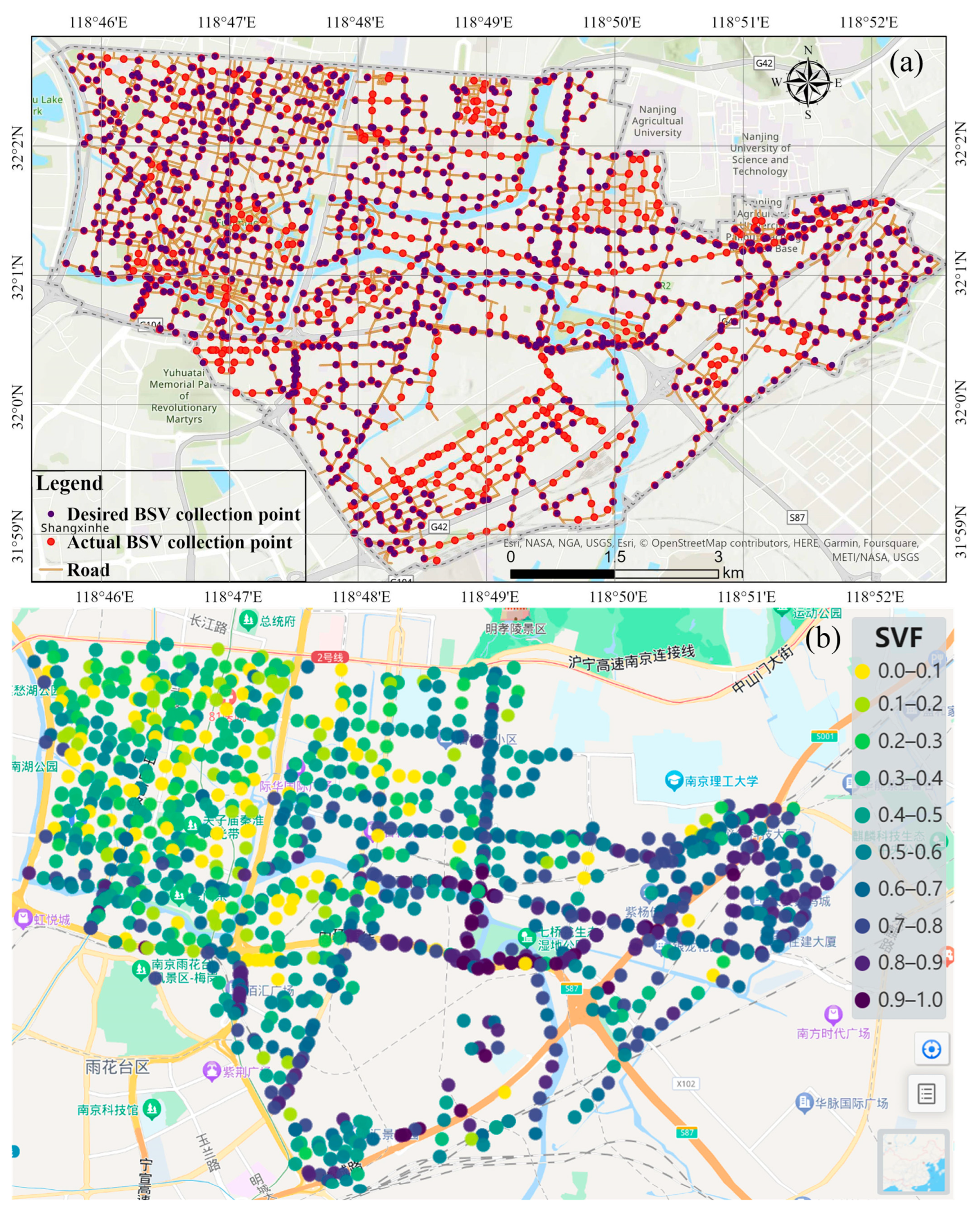
2.3. Study Area and Experimental Data

Our case study is situated in the Qinhuai District, Nanjing, China as delineated in Figure 4. Operating as one of the eight principal urban districts in Nanjing City, the Qinhuai District serves as a vital nexus for finance, business, culture, and science. By the year 2020, the district comprised 12 streets and 104 communities, spanning a total area of 49.11 km2, accommodating a resident population of 740,809. The Qinhuai District, characterized by low hills, showcases elevations decreasing towards the southeast and increasing towards the northwest. The minimum elevation is −40 m, while the maximum elevation reaches 54 m, with an average elevation of 12.82 m. The topography of the area features clearly undulating terrain, highlighting two dominant landforms—plains and hills. Additionally, the region boasts numerous surface water systems and flat terrain.
The core datasets for this study revolve around 3D buildings and urban transportation lines. The Gaode Map API facilitated the acquisition of 3D buildings and urban roads in 2019, providing crucial details and parameters currently limited to building footprints and the number of floors. The estimation of building height involved multiplying a value of 3 m per floor by the total number of floors [42,43,44]. Urban roads were categorized into four types: arterial road, branch road, expressway and trunk road, based on predefined criteria. To furnish a comprehensive understanding of the spatial distribution of buildings in the Qinhuai District, buildings were categorized into five distinct classes: low-rise building (3–9 m), multi-story building (9–21 m), middle-rise building (21–30 m), high-rise building (30–100 m) and ultra-high-rise building (>100 m), aligning with the standards outlined in the Code for Design of Civil Building—an authoritative and widely recognized standard (see Table 1).

2.4. Estimating SVF with a Simulation Method for 3D Urban Building Models

Given the low altitude of the studied area, the influence of topographical factors on this method can be disregarded. In ArcGIS Pro 3.0, the “skyline” and “skyline graph” functions are indispensable tools for visibility analysis, particularly in urban environments characterized by varying building heights [45]. The “skyline” tool identifies the visible horizon from an SVF observation point, taking into account obstructions such as 3D urban building models (see Figure 5a). This visible horizon is then depicted as the “skyline graph” (see Figure 5b), illustrating the angle of elevation to the skyline against the azimuth direction, providing a comprehensive view of the visible parts of the sky from the observer’s location. Equation (7) was utilized to ascertain SVF values from a specific SVF observation point using a generated skyline graph [26]:
S V F P A = 1 2 π s i n π 2 n i = 1 n s i n [ ( 2 i 1 ) π 2 n ] α i
where n is the total number of rings; i is the index of the ring; and αi represents the angular width of pixels of the sky in the ith ring.

3. Results

3.1. System Setting

BMapSVF stands out as an online GIS tool with a browser-based interface that enables graphical user interface interaction (see Figure 6). It seamlessly incorporates Baidu Map, a semantic segmentation model, the fisheye image projection method, and the SVF calculation method.
All features have been incorporated into the toolbox situated in the upper right corner, with the icons inside it are in SVG format:
  • Switch cities: Clicking the city list button in the top left corner initiates the switch; the map is then loaded to the corresponding city location.
  • Address search box: Address or place identification is accomplished through an automatic search in the address box. Upon clicking, the location is automatically pinpointed on the corresponding map position.
  • Panorama control: Activation of the panorama control button involves clicking and placing it on the map; revealing the covered area in the form of a blue route.
  • Location control: The positioning control button, when clicked, retrieves current position information. Preferably, the browser location interface is utilized for obtaining location information. If unsuccessful, the user IP location is invoked, and the result at the city level is returned.
  • Map toggle: Changes in map type, such as common street views, satellite views, and hybrid views of satellite and road networks, are achieved through map toggling.
  • Distance measurement: Distance measurement on the 2D map facilitates the determination of distances between measured objects.
  • Coordinate position: WGS84 and BD09 coordinates are entered into the dialog box; If the input is WGS84 coordinates, conversion to BD09 coordinates for positioning is carried out, and if it is BD09 coordinates, direct positioning occurs.
  • Sample collection: Single point sampling is executed through left-clicking, while multiple points are obtained through a csv file. SVF values are automatically calculated and stored in MySQL.
  • SVF distribution: The drawing of SVF values in colored markers on the map.
  • Map legend: The generation of symbols and colors representing SVF values.
  • Export: The exportation of results from the selected zone to a designated folder, including results in the folder and Microsoft Excel, concludes the process.
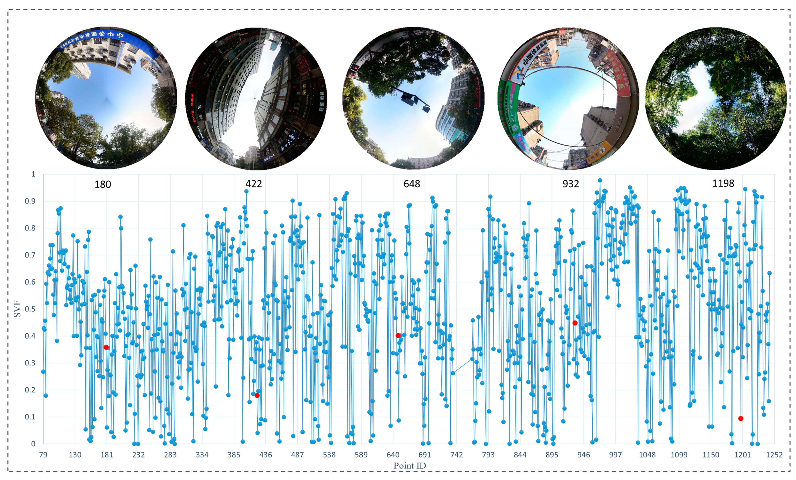
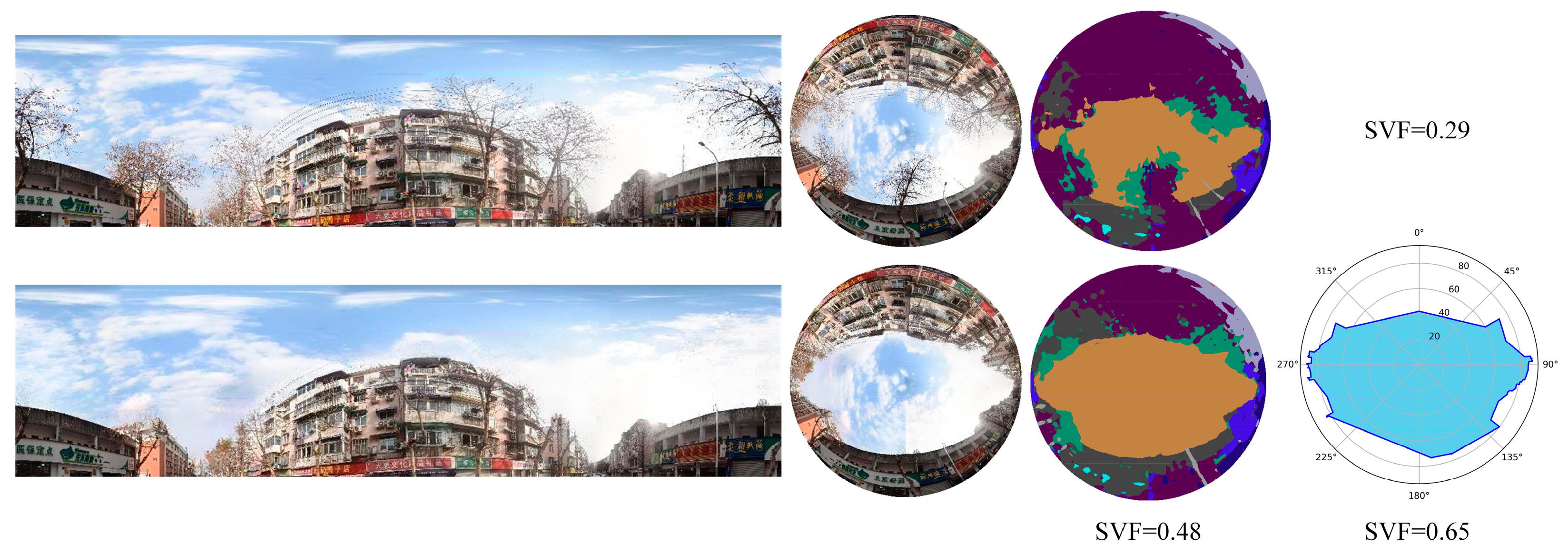
The BSV images in this study were obtained through the API of the Baidu Maps Open Platform, configuring parameters such as user access keys, field of view, image size, and latitude-longitude positions, as shown in Table 2. The maximum horizontal field of view is 360°, and the maximum vertical field of view is 180°. When the horizontal field of view is set to 360°, the image obtained through the API represents the entire panoramic view [33].
The requested parameters for BSV images, including the developer API key, image size, longitude and latitude coordinates, and horizontal field of view, are instrumental in the acquisition process. Through the BSV panorama API, URL requests are initiated to Baidu Maps, initiating a search the BSV panoramas within a specified locale and obtaining metadata in return [26] (see Figure 7). Should multiple BSV panoramas be available, the API automatically furnishes information regarding the BSV panorama in closest proximity to the input search center, with a predetermined radius of 50 m.
Within the MySQL database, the storage encompasses panoramas sourced from BSV images, accompanied by their intrinsic attribute information and the resultant SVF calculations, with the table’s fundamental structure outlined in Table 3.

3.2. Case Analysis

A total of 1433 sampling points are generated every 200 m along the road network data of the Qinhuai District, which are called the “actual BSV collection point”, SVF calculations are performed using ArcGIS Pro 3.0. The resulting longitude and latitude coordinates for each point, based on the WGS84 coordinate system, are compiled into a csv file. This file is subsequently imported into BMapSVF, initiating a search for the nearest street view image within a 25 m radius circle centered on each point, totaling 1125 sample points, called the “desired BSV collection point”. The SVF for these points is then computed, and the distribution of SVFs is visually represented across the Qinhuai District (see Figure 8).
Comprehensive data on the sampling sites collected in the Qinhuai District were stored in the database using the BMapSVF method (see Figure 9). The analysis reveals that the average and maximum SVF values were 0.51 and 0.98, respectively (see Figure 10). This observation may be attributed to the presence of fewer and sparsely distributed low-rise buildings in the southeast area of the Qinhuai District, whereas the core area exhibits a higher concentration of tall buildings, resulting in an average SVF of 0.35 with a standard deviation of 0.25.

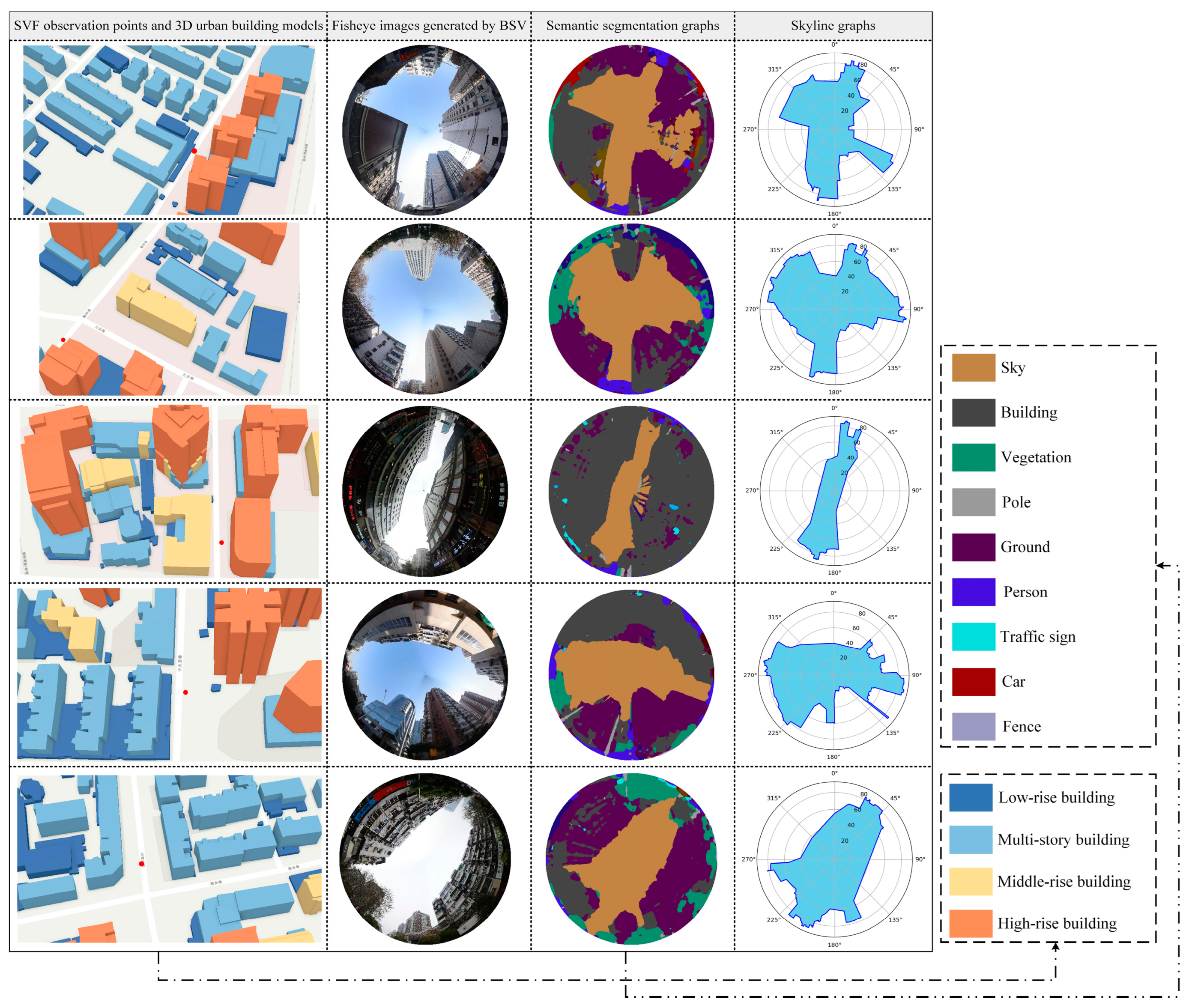
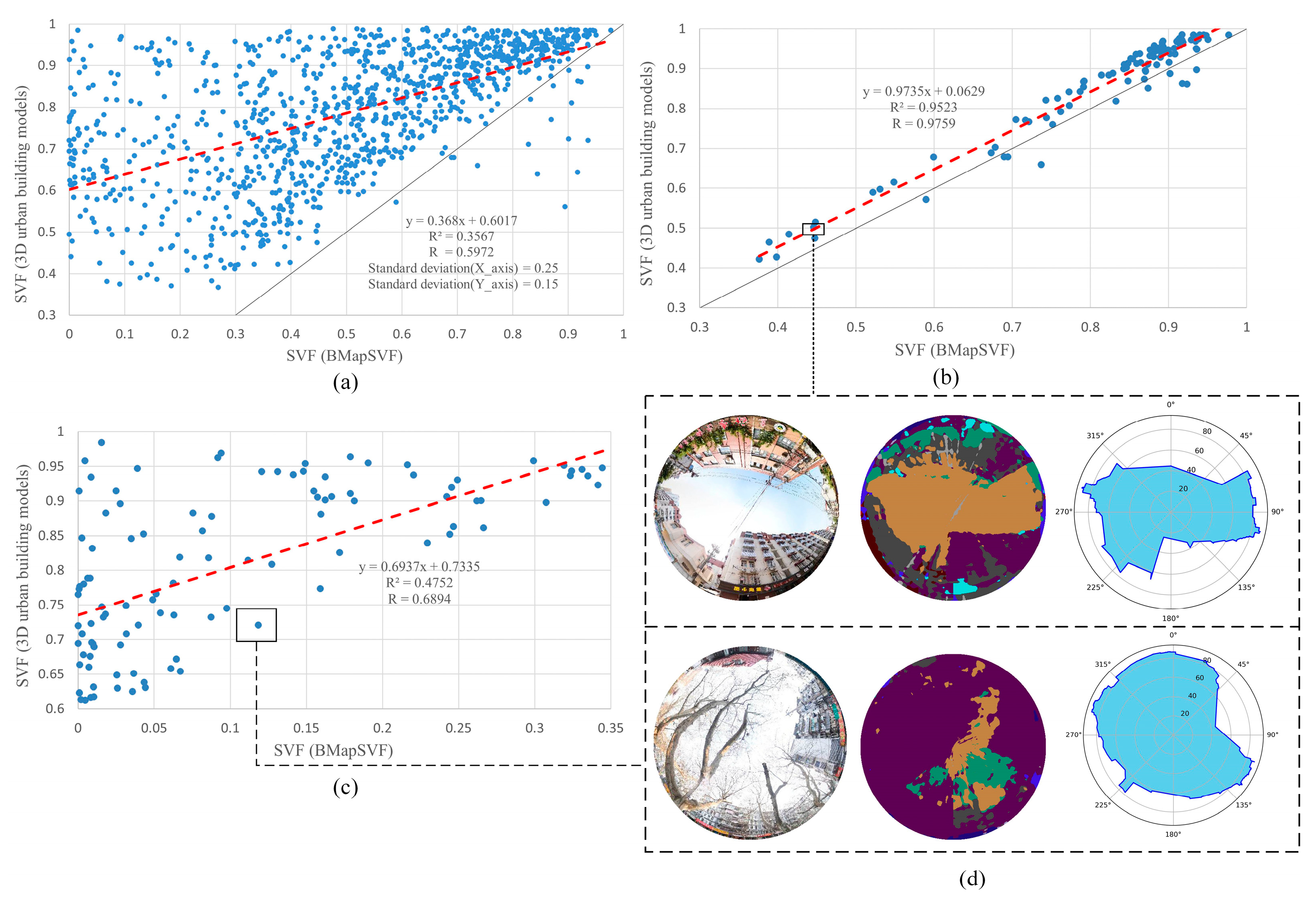
3.3. Comparison with SVF Estimation from 3D Urban Building Models

The SVF derived from BSV images is compared with results obtained from 3D urban simulations in the Qinhuai District. Firstly, the height of the camera on the BSV image acquisition vehicle is approximately 2 m. As a result, the height of the SVF 2D sampling points is standardized to 2 m and subsequently converted into 3D points. Secondly, the vector data of 2D buildings in the Qinhuai District, which includes the floor field, is multiplied by 3 to determine the height of each building, effectively transforming it into 3D buildings. The “skyline” function is then employed to generate 3D skylines, depicting the visible portion of the sky for the input SVF 3D points. Finally, based on the generated 3D skylines, the “skyline graph” tool is utilized in a separate Python script within ArcGIS Pro 3.0 to calculate the SVF value (see Figure 11).
The results demonstrate that the root mean square error (RMSE) of the SVF estimation based on the 3D urban building models and the BMapSVF method is 0.3445, the mean bias error (MBE) is −0.2816, and the correlation coefficient ® is 0.5972 (see Figure 12). The former exclusively focuses on SVF values within the architectural context, while the latter is influenced by spatial factors in complex street view images, such as trees. In the selected study area, characterized by lower tree coverage, both methods yield an RMSE of 0.0442, MBE of −0.0339, and R of 0.9784. The interval of SVF values with higher correlation is within [0.8, 1.0]. In these street view images, factors affecting the sky domain are minimal, and the geometric shape of the sky region in fisheye images is similar to that in skyline graphs. For regions with more tree coverage, the RMSE is 0.7699, MBE is 0.4642, and R is 0.6894. The correlation of SVF values is lower in these SVI, where factors influencing the sky domain are more prevalent, with trees being the most typical. When trees obstruct the sky domain, although the geometric shape of the sky region in fisheye images has some similarity with that in skyline graphs, the segmentation performance of BMapSVF for dense trees is suboptimal, leading to a decrease in SVF estimation. This paper refers to these influencing factors as spatial uncertainty.

3.4. The Uncertainty of the SVF

The concept of spatial uncertainty is introduced to describe the factors influencing the visible range of the sky in SVI, including trees that change with the seasons, traffic signs, and wires. This allows for a more accurate estimation of the SVF. The impact of spatial uncertainty on BSV scarcely alters the sky range, and SVF values obtained through both approaches appear comparable when the sky openness is moderately high. However, when spatial uncertainty exerts significant influence, it leads to considerable divergence in the estimated SVF (see Figure 13). This intervention forms the basis of our forthcoming research.
Furthermore, despite the higher semantic segmentation accuracy provided by deep neural networks, there is uncertainty introduced in the estimation of SVF, encompassing both data uncertainty and model uncertainty. Data uncertainty may arise from disparities between the source and target domains of SVI, representing an inherent attribute of data distribution. Model uncertainty is introduced by deep neural networks. Mukhoti et al. integrated a Bayesian neural network incorporating MC dropout and Concrete dropout strategies into DeepLabv3+ to qualitatively and quantitatively assess uncertainty (see Figure 14) [46]. In future work, we will delve deeper into studying the impact of data uncertainty and model uncertainty from deep neural networks on SVF estimation in SVI. It aims to analyze the sensitivity of SVF values to variations in uncertainty.

4. Discussion

In a certain sense, with the continuous and extensive coverage of BSV, BMapSVF enables the real-time collection of numerous panoramic images for calculation SVF values and generates corresponding spatial databases for the respective areas. The SVF values computed using BMapSVF can contribute to a better understanding of urban morphological characteristics. Moreover, they can be further utilized to investigate the relationships between the SVF and urban heat island effects, solar radiation, spatial environmental quality, and other factors. These findings provide a scientific basis for rational urban planning and development, offering valuable insights for decision-making processes.
Although it is not difficult for urban researchers to calculate the SVF using simple scripts, BMapSVF offers more ease of operation and user-friendliness in an online and visualized format that can be used in a browser as soon as it is deployed. Users can see the fisheye image and SVF values for each sampling point on the map. As of now, BMapSVF can be applied to different urban environments in China. The validation in this study was conducted in a research area with relatively dense building structures. To obtain test data for different urban environments, the source code of this tool has been made available in this paper, enabling users to enhance the adaptability of BMapSVF across diverse urban settings. The correct use of this tool requires the user to upload the correct sampling point file or to sample a single point directly on Baidu Map to ensure that the other functions work properly.
During the semantic segmentation of BSV panoramas, we found that our prediction model had limited capability in representing vegetation features, especially with seasonal variations. The density and coverage of vegetation significantly affect the estimation of the SVF. Therefore, it might be necessary to improve the ability of the model to accurately segment vegetation, particularly in complex scenes to obtain high-precision SVF values.
In Section 3.3, the 3D urban building models-based method was employed to compute the SVF; the results indicated a significant discrepancy between the two methods. In a study conducted by [28], the SVF estimated based on the LiDAR-Derived Digital Surface Model (DSM) was compared with the SVF estimated from SVI, yielding a correlation coefficient of 0.2818. Subsequently, we considered the influence of vegetation factors and obtained a correlation coefficient of 0.5972.
The SVF estimation method based on 3D urban building models uses building floor numbers provided by Gaode Map without considering trees factors. The significant difference between the proposed method and the SVF estimation method based on BSV images can also be attributed to this factor. This indirectly reflects that Gaode Map offers a rapid channel for acquiring three-dimensional building data, presenting considerable advantages in utilizing online resources for SVF calculations. In addition, the time of street view image acquisition and the change in building data will also affect the results of SVF estimation.
In urban scenes, the SVF value is affected by spatial uncertainty factors, especially the occlusion of trees. In general, quantitatively describing the impact of trees is a challenging issue in SVF studies. The complex geometrical shapes of trees and the seasonal changes in crown volume caused by leaf growth and falling leaves force researchers to ignore trees or apply simple geometric objects [47]. Therefore, SVI will still be employed as a data source, studying to further quantify the effect of trees on the accuracy of the SVF and to remove trees based on the context of the image in the future. We will consider more factors to continuously improve the accuracy of extracting SVF values from SVI.

5. Conclusions

This study presents the development of BMapSVF, and the source code, demo, and models are publicly available at https://github.com/Voyagerlemon/BMapSVF (accessed on 12 December 2023). It is a novel tool for easily obtaining SVF information from the massive BSV panorama database in developed cities in China. The tool is demonstrated through a complex environmental scenario in the Qinhuai District, aiming to enable fast computation of the SVF for large urban areas and further analysis of the spatial distribution of the SVF.
In all sampling points within the Qinhuai District, SVF estimation occurs through methods based on both 3D urban building models and BMapSVF, resulting in an RMSE of 0.3445, an MBE of −0.2816, and an R of 0.5972. At sampling points with limited tree coverage, the RMSE of the SVF estimates from both methods is 0.0442, the MBE is −0.0339, and the R is 0.9784. Conversely, at sampling points with substantial tree coverage, the RMSE of the SVF estimates from both methods is 0.7699, the MBE is 0.4642, and the R is 0.6894.
Within the complexities of urban settings, BMapSVF excels in delivering more refined estimations of the SVF. However, it is imperative to consider spatial uncertainty factors, particularly in the context of tree obstructions. This consideration may result in a decline in SVF values estimated through BMapSVF, further illustrating that the spatial structure of this region is more diversified than that of other urban areas.
In general, BMapSVF efficiently extracts the SVF using online map data resources, resolving limitations in online, large-scale, and rapid SVF estimation capabilities. Given that this tool has undergone testing solely in existing scenarios, users may need to assess its applicability under diverse conditions. Furthermore, the tool incorporates the intelligent retrieval of other urban spatial data, offering users flexibility based on their specific requirements.

Author Contributions

Conceptualization, H.L.; Data curation, H.X. and S.L.; Formal analysis, H.X.; Methodology, H.X., H.L. and S.L.; Software, H.X.; Supervision, H.L.; Validation, H.X.; Writing—original draft, H.X.; Writing—review and editing, H.L. All authors have read and agreed to the published version of the manuscript.

Funding

This research was funded by the National Natural Science Foundation of China, grant number 41478324.

Institutional Review Board Statement

Not applicable.

Informed Consent Statement

Not applicable.

Data Availability Statement

The study did not report any publicly archived datasets, please refer to the GitHub repository provided in this paper for specific details.

Conflicts of Interest

The authors declare no conflicts of interest.

References

  1. Middel, A.; Lukasczyk, J.; Maciejewski, R.; Demuzere, M.; Roth, M. Sky View Factor footprints for urban climate modeling. Urban Clim. 2018, 25, 120–134. [Google Scholar] [CrossRef]
  2. Poon, K.H.; Kmpf, J.H.; Tay, S.; Wong, N.H.; Reindl, T.G. Parametric study of URBAN morphology on building solar energy potential in Singapore context. Urban Clim. 2020, 33, 100624. [Google Scholar] [CrossRef]
  3. Santos Nouri, A.; Costa, J.P.; Matzarakis, A. Examining default urban-aspect-ratios and sky-view-factors to identify priorities for thermal-sensitive public space design in hot-summer Mediterranean climates: The Lisbon case. Build. Environ. 2017, 126, 442–456. [Google Scholar] [CrossRef]
  4. He, X.D.; Miao, S.G.; Shen, S.H.; Li, J.; Zhang, B.Z.; Zhang, Z.Y.; Chen, X.J. Influence of sky view factor on outdoor thermal environment and physiological equivalent temperature. Int. J. Biometeorol. 2015, 59, 285–297. [Google Scholar] [CrossRef]
  5. Zhang, J.; Gou, Z.H.; Lu, Y.; Lin, P.Y. The impact of sky view factor on thermal environments in urban parks in a subtropical coastal city of Australia. Urban For. Urban Green. 2019, 44, 18. [Google Scholar] [CrossRef]
  6. Zheng, B.H.; Li, J.Y. Evaluating the Annual Effect of the Sky View Factor on the Indoor Thermal Environment of Residential Buildings by Envi-met. Buildings 2022, 12, 787. [Google Scholar] [CrossRef]
  7. Ge, J.; Wang, Y.; Akbari, H.; Zhou, D. The effects of sky view factor on ground surface temperature in cold regions—A case from Xi’an, China. Build. Environ. 2022, 210, 108707. [Google Scholar] [CrossRef]
  8. Oke, T.R. Canyon geometry and the nocturnal urban heat island: Comparison of scale model and field observations. J. Climatol. 1981, 1, 237–254. [Google Scholar] [CrossRef]
  9. Unger, J. Intra-urban relationship between surface geometry and urban heat island: Review and new approach. Clim. Res. 2004, 27, 253–264. [Google Scholar] [CrossRef]
  10. Zhu, S.Y.; Guan, H.D.; Bennett, J.; Clay, R.; Ewenz, C.; Benger, S.; Maghrabi, A.; Millington, A.C. Influence of sky temperature distribution on sky view factor and its applications in urban heat island. Int. J. Climatol. 2013, 33, 1837–1843. [Google Scholar] [CrossRef]
  11. Chiang, Y.-C.; Liu, H.-H.; Li, D.; Ho, L.-C. Quantification through deep learning of sky view factor and greenery on urban streets during hot and cool seasons. Landsc. Urban Plan. 2023, 232, 104679. [Google Scholar] [CrossRef]
  12. Chen, L.; Ng, E.; An, X.P.; Ren, C.; Lee, M.; Wang, U.; He, Z.J. Sky view factor analysis of street canyons and its implications for daytime intra-urban air temperature differentials in high-rise, high-density urban areas of Hong Kong: A GIS-based simulation approach. Int. J. Climatol. 2012, 32, 121–136. [Google Scholar] [CrossRef]
  13. Song, B.G. Comparison of thermal environments and classification of physical environments using fisheye images with object-based classification. Urban Clim. 2023, 49, 101510. [Google Scholar] [CrossRef]
  14. Wei, R.; Song, D.; Wong, N.H.; Martin, M. Impact of urban morphology parameters on microclimate. Procedia Eng. 2016, 169, 142–149. [Google Scholar] [CrossRef]
  15. Johnson, G.T.; Watson, I.D. The Determination of view-factors in urban canyons. J. Clim. Appl. Meteorol. 1984, 23, 329–335. [Google Scholar] [CrossRef]
  16. Watson, I.D.; Johnson, G.T. Graphical estimation of sky view-factors in urban environments. J. Climatol. 1987, 7, 193–197. [Google Scholar] [CrossRef]
  17. Grimmond, C.S.B.; Potter, S.K.; Zutter, H.N.; Souch, C. Rapid methods to estimate sky-view factors applied to urban areas. Int. J. Climatol. 2001, 21, 903–913. [Google Scholar] [CrossRef]
  18. Honjo, T.; Tzu-Ping, L.; Seo, Y. Sky view factor measurement by using a spherical camera. J. Agric. Meteorol. 2019, 75, 59–66. [Google Scholar] [CrossRef]
  19. Matzarakis, A.; Matuschek, O. Sky view factor as a parameter in applied climatology—Rapid estimation by the SkyHelios model. Meteorol. Z. 2011, 20, 39–45. [Google Scholar] [CrossRef]
  20. Chapman, L.; Thornes, J.E. Real-time sky-view factor calculation and approximation. J. Atmos. Ocean. Technol. 2004, 21, 730–741. [Google Scholar] [CrossRef]
  21. Chapman, L.; Thornes, J.E.; Bradley, A.V. Sky-view factor approximation using GPS receivers. Int. J. Climatol. 2002, 22, 615–621. [Google Scholar] [CrossRef]
  22. Cheung, H.K.W.; Coles, D.; Levermore, G.J. Urban heat island analysis of Greater Manchester, UK using sky view factor analysis. Build Serv. Eng. Res. Technol. 2016, 37, 5–17. [Google Scholar] [CrossRef]
  23. Liang, J.M.; Gong, J.H.; Xie, X.P.; Sun, J. Solar3D: An Open-Source Tool for Estimating Solar Radiation in Urban Environments. ISPRS Int. Geo-Inf. 2020, 9, 524. [Google Scholar] [CrossRef]
  24. Zeng, L.Y.; Lu, J.; Li, W.Y.; Li, Y.C. A fast approach for large-scale Sky View Factor estimation using street view images. Build. Environ. 2018, 135, 74–84. [Google Scholar] [CrossRef]
  25. Yang, J.; Wong, M.S.; Menenti, M.; Nichol, J. Modeling the effective emissivity of the urban canopy using sky view factor. ISPRS J. Photogramm. Remote Sens. 2015, 105, 211–219. [Google Scholar] [CrossRef]
  26. Wang, Z.A.; Tang, G.A.; Lu, G.N.A.; Ye, C.; Zhou, F.Z.; Zhong, T. Positional error modeling of sky-view factor measurements within urban street canyons. Trans. GIS 2021, 25, 1970–1990. [Google Scholar] [CrossRef]
  27. Carrasco-Hernandez, R.; Smedley, A.R.D.; Webb, A.R. Using urban canyon geometries obtained from Google Street View for atmospheric studies: Potential applications in the calculation of street level total shortwave irradiances. Energy Build. 2015, 86, 340–348. [Google Scholar] [CrossRef]
  28. Liang, J.M.; Gong, J.H.; Sun, J.; Zhou, J.P.; Li, W.H.; Li, Y.; Liu, J.; Shen, S. Automatic Sky View Factor Estimation from Street View Photographs-A Big Data Approach. Remote Sens. 2017, 9, 411. [Google Scholar] [CrossRef]
  29. Badrinarayanan, V.; Kendall, A.; Cipolla, R. Segnet: A deep convolutional encoder-decoder architecture for image segmentation. IEEE Trans. Pattern Anal. Mach. Intell. 2017, 39, 2481–2495. [Google Scholar] [CrossRef]
  30. Gong, F.Y.; Zeng, Z.C.; Zhang, F.; Li, X.J.; Ng, E.; Norford, L.K. Mapping sky, tree, and building view factors of street canyons in a high-density urban environment. Build. Environ. 2018, 134, 155–167. [Google Scholar] [CrossRef]
  31. Xia, Y.X.; Yabuki, N.; Fukuda, T. Sky view factor estimation from street view images based on semantic segmentation. Urban Clim. 2021, 40, 14. [Google Scholar] [CrossRef]
  32. Chen, L.-C.; Zhu, Y.; Papandreou, G.; Schroff, F.; Adam, H. Encoder-decoder with atrous separable convolution for semantic image segmentation. In Proceedings of the European Conference on Computer Vision (ECCV), Munich, Germany, 8–14 September 2018; pp. 801–818. [Google Scholar]
  33. Feng, Y.; Chen, L.; He, X. Sky View Factor Calculation based on Baidu Street View Images and Its Application in Urban Heat Island Study. J. Geo-Inf. Sci. 2021, 23, 1998–2012. [Google Scholar] [CrossRef]
  34. Liang, J.M.; Gong, J.H.; Zhang, J.M.; Li, Y.; Wu, D.; Zhang, G.Y. GSV2SVF-an interactive GIS tool for sky, tree and building view factor estimation from street view photographs. Build. Environ. 2020, 168, 106475. [Google Scholar] [CrossRef]
  35. BSV Baidu Street View. Available online: https://lbs.baidu.com/faq/api?title=viewstatic-base (accessed on 30 August 2023).
  36. Chen, L.-C.; Papandreou, G.; Schroff, F.; Adam, H. Rethinking atrous convolution for semantic image segmentation. arXiv 2017, arXiv:1706.05587. [Google Scholar] [CrossRef]
  37. Cordts, M.; Omran, M.; Ramos, S.; Rehfeld, T.; Schiele, B. The Cityscapes Dataset for Semantic Urban Scene Understanding. In Proceedings of the IEEE Conference on Computer Vision and Pattern Recognition (CVPR), Las Vegas, NV, USA, 27–30 June 2016; pp. 3213–3223. [Google Scholar] [CrossRef]
  38. Zhao, Z.; Chen, Y.; Liu, J.; Shen, Z.; Liu, M. Cross-people mobile-phone based activity recognition. In Proceedings of the Twenty-Second International Joint Conference on Artificial Intelligence, Barcelona, Spain, 16–22 July 2011. [Google Scholar]
  39. Tan, C.; Sun, F.; Kong, T.; Zhang, W.; Yang, C.; Liu, C. A survey on deep transfer learning, Artificial Neural Networks and Machine Learning. In Proceedings of the 27th International Conference on Artificial Neural Networks, ICANN 2018, Rhodes, Greece, 4–7 October 2018; Proceedings, Part III 27; Springer International Publishing: Berlin/Heidelberg, Germany, 2018; pp. 270–279. [Google Scholar] [CrossRef]
  40. Li, X.J.; Ratti, C.; Seiferling, I. Quantifying the shade provision of street trees in urban landscape: A case study in Boston, USA, using Google Street View. Landsc. Urban Plan. 2018, 169, 81–91. [Google Scholar] [CrossRef]
  41. Pimentel, V.; Nickerson, B.G. Communicating and displaying real-time data with websocket. IEEE Internet Comput. 2012, 16, 45–53. [Google Scholar] [CrossRef]
  42. He, S.J.; Wang, X.Y.; Dong, J.R.; Wei, B.C.; Duan, H.M.; Jiao, J.Z.; Xie, Y.W. Three-Dimensional Urban Expansion Analysis of Valley-Type Cities: A Case Study of Chengguan District, Lanzhou, China. Sustainability 2019, 11, 5663. [Google Scholar] [CrossRef]
  43. Koziatek, O.; Dragicevic, S. A local and regional spatial index for measuring three-dimensional urban compactness growth. Envrion. Plan. B-Urban Anal. CIty Sci. 2019, 46, 143–164. [Google Scholar] [CrossRef]
  44. Yang, L.; Yang, X.; Zhang, H.P.; Ma, J.F.; Zhu, H.; Huang, X. Urban morphological regionalization based on 3D building blocks-A case in the central area of Chengdu, China. Comput. Environ. Urban Syst. 2022, 94, 101800. [Google Scholar] [CrossRef]
  45. Park, C.; Ha, J.; Lee, S. Association between Three-Dimensional Built Environment and Urban Air Temperature: Seasonal and Temporal Differences. Sustainability 2017, 9, 1338. [Google Scholar] [CrossRef]
  46. Mukhoti, J.; Gal, Y. Evaluating bayesian deep learning methods for semantic segmentation. arXiv 2018, arXiv:1811.12709. [Google Scholar]
  47. An, S.M.; Kim, B.S.; Lee, H.Y.; Kim, C.H.; Yi, C.Y.; Eum, J.H.; Woo, J.H. Three-dimensional point cloud based sky view factor analysis in complex urban settings. Int. J. Climatol. 2014, 34, 2685–2701. [Google Scholar] [CrossRef]
Figure 1. Example of the complex spatial information and multiscale phenomenon in SVI.
Applsci 14 02133 g001
Figure 2. Flow of SVF calculation based on BSV, the red dots represent the sampling points.
Applsci 14 02133 g002
Figure 3. BMapSVF system architecture.
Applsci 14 02133 g003
Figure 4. Study area: (a) positional maps featuring 3D buildings and the network of urban roads; and (b) The digital elevation model (DEM) specific to the study area.
Applsci 14 02133 g004
Figure 5. Estimation of the SVF with ArcGIS built-in tools: (a) the skyline of the SVF observation point is generated through the 3D urban building model; and (b) the skyline graph of the observing point with the SVF value.
Applsci 14 02133 g005
Figure 6. The user interface of BMapSVF.
Applsci 14 02133 g006
Figure 7. An example of a BSV panorama and its corresponding metadata collected on Fuhua Rd., Shenzhen City: (a) an illustration of the BSV panorama API request URL and the subsequent return of the BSV panorama; and (b) an illustration of the BSV panorama API request URL and the resulting metadata for the BSV panorama. This image and metadata were accessed through this URL: http://api.map.baidu.com/panorama/ (accessed on 23 September 2023).
Applsci 14 02133 g007
Figure 8. Visualization of the SVF distribution in the Qinhuai District: (a) the road network, establishing designated BSV collection points with their actual locations determined using BMapSVF; and (b) the representation of the spatial distribution of SVF on BMapSVF using ten colors from the Viridis color spectrum.
Applsci 14 02133 g008
Figure 9. Table schema of the BMapSVF database.
Applsci 14 02133 g009
Figure 10. Statistical analysis of the SVF proportions for the Qinhuai District, the blue dots represent the SVF for each sampling point, while the red dots serve as an example of SVF with significant variations due to factors such as trees and buildings causing obstruction.
Applsci 14 02133 g010
Figure 11. Fisheye images and the corresponding skyline graphs at the sampling points, the red dots represent the sampling points.
Applsci 14 02133 g011
Figure 12. The relationship between the SVF estimated based on BMapSVF and that based on the 3D urban building models: (a) comparing the results of two SVF approximation methods that consider spatial uncertainty; (b) exploring the relationship between the two methods in scenarios where trees are sparsely distributed in BSV images; (c) investigating the relationship between the two methods in cases with abundant trees in BSV images; and (d) offering examples depicting fisheye images and skyline graphs for both sparse and dense tree scenarios.
Applsci 14 02133 g012
Figure 13. Pre- and post-comparison images and SVF values for removing spatial uncertainty in BSV.
Applsci 14 02133 g013
Figure 14. Uncertainty results of semantic segmentation networks in SVI. Predictive entropy maps represent qualitative results of uncertainty. Darker shades indicate higher uncertainty [46].
Applsci 14 02133 g014
Table 1. The classification of buildings is conducted based on their respective heights.
ClassificationHeight (m)CountRatio
Low-rise building3–927,13056.31%
Multi-story building9–2113,92628.90%
Middle-rise building21–3039978.30%
High-rise building30–10030556.34%
Ultra-high-rise building>100740.15%
Table 2. Required parameters of URL.
ParametersDescription
akAPI key
widthpanorama width
heightpanorama height
locationpanorama location coordinates (longitude, latitude)
fovhorizontal direction range, range [10°, 360°]
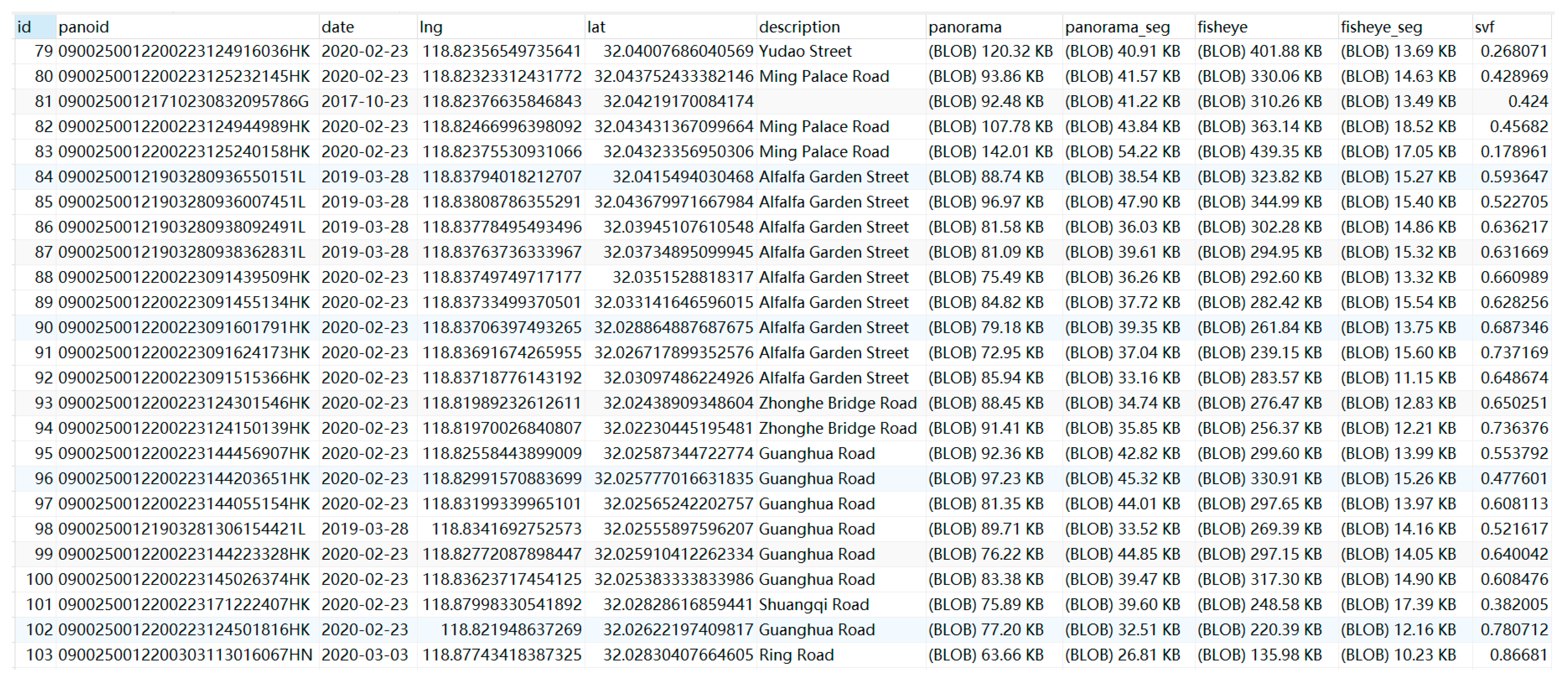
Table 3. Data structure table.
FieldField TypeNot NullDescription
idintyeskey
panoidvarcharyesthe panorama id
datedateyesacquisition of the BSV panorama
lngdoubleyesBD09 longitude
latdoubleyesBD09 latitude
descriptionvarcharnoPanorama road name
panoramalongblobyesBLOB format the BSV panorama
panorama_seglongblobyessemantic segmentation images of panoramas
fisheyelongblobyesfisheye images of panoramas
fisheye_seglongblobyesfisheye images of panorama_seg
svffloatyesSVF is calculated by BMapSVF
Disclaimer/Publisher’s Note: The statements, opinions and data contained in all publications are solely those of the individual author(s) and contributor(s) and not of MDPI and/or the editor(s). MDPI and/or the editor(s) disclaim responsibility for any injury to people or property resulting from any ideas, methods, instructions or products referred to in the content.

