Quality Analysis of Unmanned Aerial Vehicle Images Using a Resolution Target

Abstract

Unmanned aerial vehicle (UAV) photogrammetry is an emerging means of acquiring high-precision rapid spatial information and data because it is cost-effective and highly efficient. However, securing uniform quality in the results of UAV photogrammetry is difficult due to the use of low-cost navigation devices, non-surveying cameras, and rapid changes in shooting locations depending on the aircraft’s behavior. In addition, no specific procedures or guidelines exist for performing quantitative quality tests or certification methods on UAV images. Additionally, test tools for UAV image quality assessment only use the ground sample distance (GSD), often resulting in a reduced image quality compared with that of manned aircraft images. In this study, we performed a modulation transfer function (MTF) analysis using a slanted edge target and a GSD analysis to confirm the necessity of MTF analysis in UAV image quality assessments. In this study, we aimed to address this issue by conducting a modulation transfer function (MTF) analysis using a slanted edge target and a ground sample distance (GSD) analysis. This was carried out to confirm the necessity of MTF analysis in evaluating UAV image quality. Furthermore, we analyzed the impact of flight height and mounted sensors on image quality at different study sites.

1. Introduction

Images obtained using unmanned aerial vehicles (UAVs) are captured at low heights, and thus, have higher resolutions than those captured by manned aircraft and can be acquired anytime and anywhere. Additionally, UAVs are emerging as a means of acquiring high-precision rapid spatial information and data because of their low cost and high efficiency. Images obtained from UAVs are widely used in public and private institutions for surveying civil engineering and construction sites [1,2], estimating the quantity of civil works, analyzing terrain slope, in traffic applications for traffic data collection [3,4,5], are utilized in agriculture and for the environment [6,7,8] and coastline detection, and find application in the marine field [9,10] and in studying forest diseases and pests [11]. Therefore, practical applicable operational procedures such as public surveying have been established. However, it is difficult to obtain data with consistent quality and to use UAV images in practical applications because no specific procedures or methods exist for quantitatively testing or certifying the data’s quality. This difficulty has been attributed to the use of cheap navigation systems, the unsteadiness of the UAV at the time of image capture, and unfavorable weather conditions. In addition, ground sample distance (GSD) analysis is currently used for assessing the image quality [12].

Several methods are used for testing UAV image quality, including the MTF, edge response, and GSD analyses. Among previous studies on aerial image quality testing, Baer [13] proposed the spatial resolution analysis method using a circular target. The method overcomes the shortcomings of the traditional method that uses edge and slanted edge targets. Wang et al. [14] proposed a method that automatically measures the modulation transfer function (MTF) with a high success rate and acceptable accuracy using the Hough transform for detecting straight lines from manned aircraft or satellite images. Sieberth et al. [15] developed a technique that automatically filters UAV image blurring caused by camera movements induced by strong wind, turbulence, or the operator’s sudden movement. The technique enables objective analysis as it automatically detects and removes blurring from UAV images, improves image quality, and reduces time and cost compared to the traditional method based on manual detection by the operator. Orych [16] used the Siemens star to measure spatial resolution in UAV images. The Siemens star facilitates analysis and ensures objectivity in all directions as it is unaffected by flight direction. Additionally, as the Siemens star has a smaller size and smaller dimensions than those of the bar target, which is widely used for manned aircraft images, the Siemens star is an ideal resolution target for the UAV photogrammetry system, which flies at low heights. Likewise, many methods are used for testing UAV image quality, including the MTF, edge response, and GSD analyses.

However, the quality of UAV images is lower than that of manned aircraft images, in some cases because the UAV image quality test tool assesses quality using only the GSD analysis, which, unlike the MTF or edge response analyses, does not consider the contrast levels alongside image resolution. In addition, securing uniform quality in the results of UAV photogrammetry is difficult due to the use of low-cost navigation devices, non-surveying cameras, and rapid changes in shooting locations depending on the aircraft’s behavior.

To address this issue, we aimed to investigate the effect of UAV imaging altitude and the performance of mounting sensors on UAV imaging quality. We also aimed to evaluate the necessity of MTF analysis in evaluating UAV imaging quality. To achieve this, we set up inclined corners and bar targets at the shooting site, as shown in Figure 1, and captured images using four types of UAVs and one type of manned aircraft. We conducted shooting using different mounting sensors at the same shooting altitude, and the same mounting sensors were also used at different shooting heights. Subsequently, we generated the final UAV orthoimages and performed both GSD and MTF analyses on the corresponding orthoimages to draw conclusions.

2. Theoretical Background

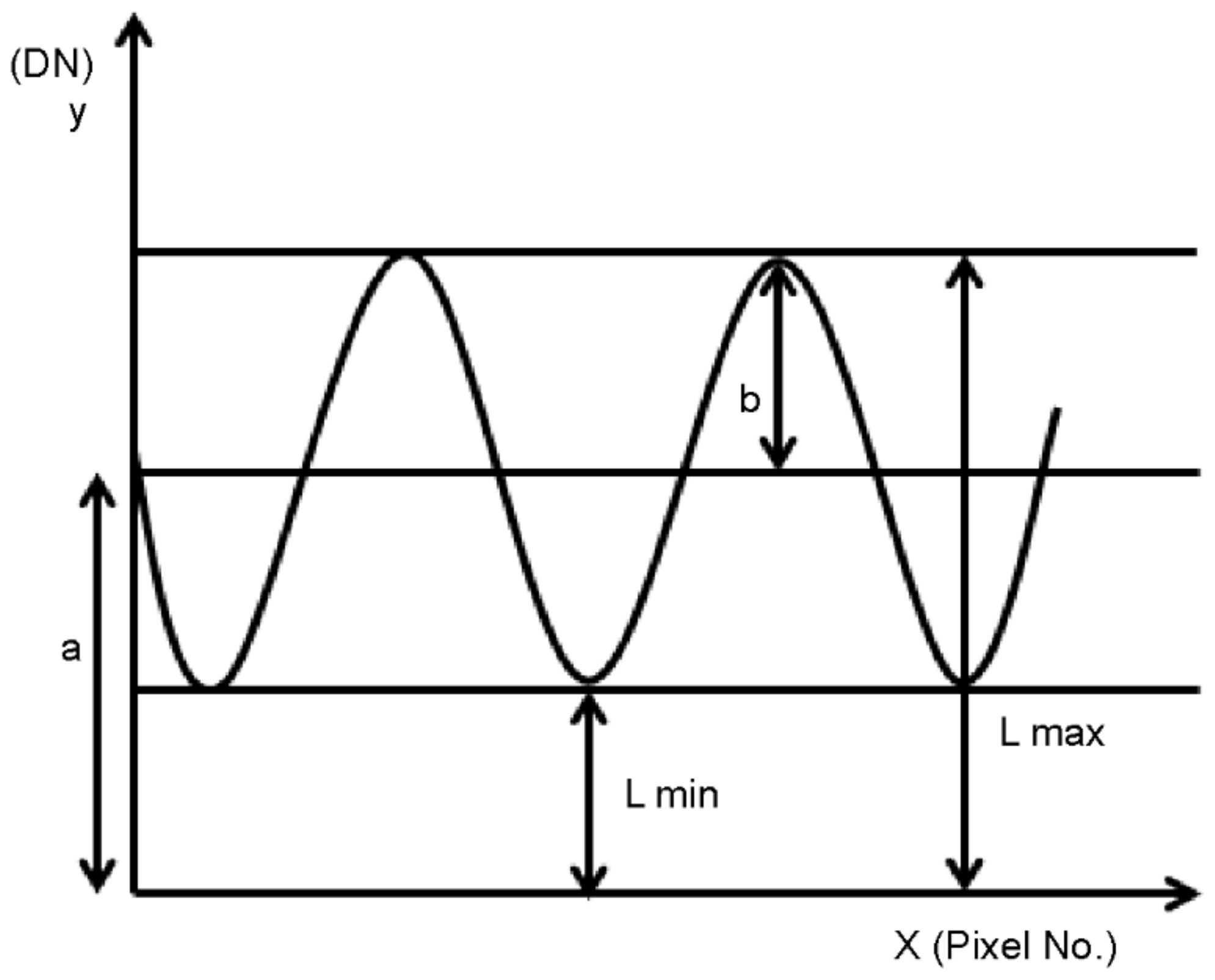
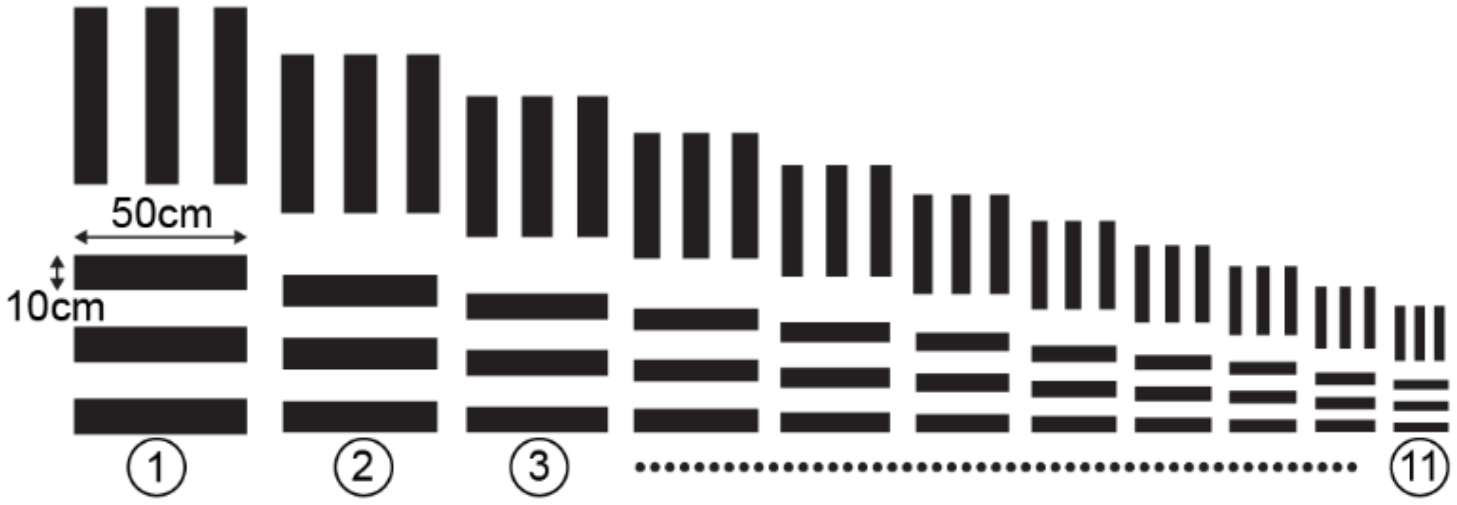
2.1. GSD Analysis Using the Bar Target

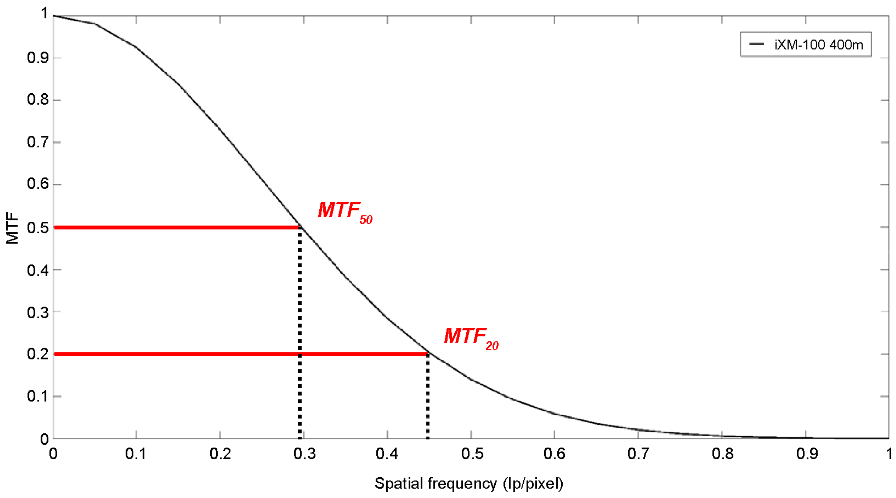
We analyzed the GSD using a bar target in addition to the MTF to determine the image resolution and contrast. We compared the results to determine the necessity of MTF analysis. The spatial resolution analysis using the bar target is described below. As illustrated in Figure 2, the modulation function in an image can be represented by digital numbers (DNs), which are not continuous for each pixel in the original image [17].

When a graph of numbers in non-continuous points is fitted by the method of least squares, the curve is expressed as a sine function in periodic form, such as Equation (1):

$$\mathrm{Y}=\mathrm{a}+\mathrm{b}\sin \omega (x-x_0),$$

(1)

where a is a coefficient for the digital numbers (DNs) in a pixel from which a curve begins before it moves toward the y-intercept; $\mathrm{b}$ represents the amplitude of the sine curve, i.e., the difference between the maximum and minimum values; $\omega$ represents the period of the sine function and is related to the image GSD measurement; $x$ represents the pixel sequence; and $x_0$ is the distance moved in parallel toward the x-axis, causing a phase change that determines the form of the sine function. Hence, an accurate image GSD can be obtained by measuring the size of the black and white lines in the imaged target and dividing the size by the spatial frequency represented in the sine function with the coefficients calculated from Equation (1).

2.2. MTF Analysis

Cameras do not provide images that perfectly represent real objects. object’s level of representation is related to the camera’s performance; the MTF value, which indicates the object’s level of representation, is used for analyzing UAV images. The MTF analysis is based on the camera’s lens and performance. The MTF value is expressed as the relative ratio of the actual modulation value of the resolution target to the modulation value of the target in an image. The MTF can be analyzed using a graph based on spatial frequency, which shows how many line pairs (lps) can be included in one pixel when black and white lines form each lp. In the MTF graph, the horizontal axis expresses spatial frequency, and the vertical axis expresses the MTF value [18].

Figure 3 illustrates the DNs extracted from an image with black and white line pairs. In this graph, the modulation value is expressed by Equation (2):

$$\mathrm{M}\mathrm{o}\mathrm{d}\mathrm{u}\mathrm{l}\mathrm{a}\mathrm{t}\mathrm{i}\mathrm{o}\mathrm{n}=\frac{l_{max}-l_{min}}{l_{max}+l_{min}}=\frac{a+b-(a-b)}{a+b+\left(a-b\right)}=\frac{2b}{2a}=\frac{a}{b}$$

(2)

The MTF value is expressed by Equation (3):

$$\mathrm{M}\mathrm{T}\mathrm{F}=\frac{{Modulation}_{Image}}{{Modulation}_{Object}},$$

(3)

where ${Modulation}_{Image}$ is the modulation value of the image, and ${Modulation}_{Object}$ is the modulation value extracted from the actual object.

$$\mathrm{M}\mathrm{T}\mathrm{F}=e^{-2{\pi }^2{{\sigma }^2}_{MTF}{K}^2},$$

(4)

The DNs extracted from UAV images taken by the iXM-100 sensor, as illustrated in Figure 4, were linearized, and an MTF graph was generated using Equation (4), where K represents the spatial frequency equivalent to the vertical axis of the MTF, and ${{\sigma }^2}_{MTF}$ is the variance of the MTF [19].

We calculated ${\sigma }_{MTF}$, the standard deviation of the MTF, and performed comparisons. We also calculated and compared ${MTF}_{50}$, a spatial frequency equivalent to 50% of the MTF graph, and ${MTF}_{20}$, a spatial frequency equivalent to 20% of the MTF graph, as illustrated in Figure 4. ${MTF}_{50}$ is an empirical criterion used in many studies, and it refers to a spatial frequency from which the boundary begins to blur in the operator’s eyes. ${MTF}_{20}$ refers to the minimum spatial frequency at which the boundary is distinguishable by the operator’s eyes. It is also an empirical criterion used in many studies.

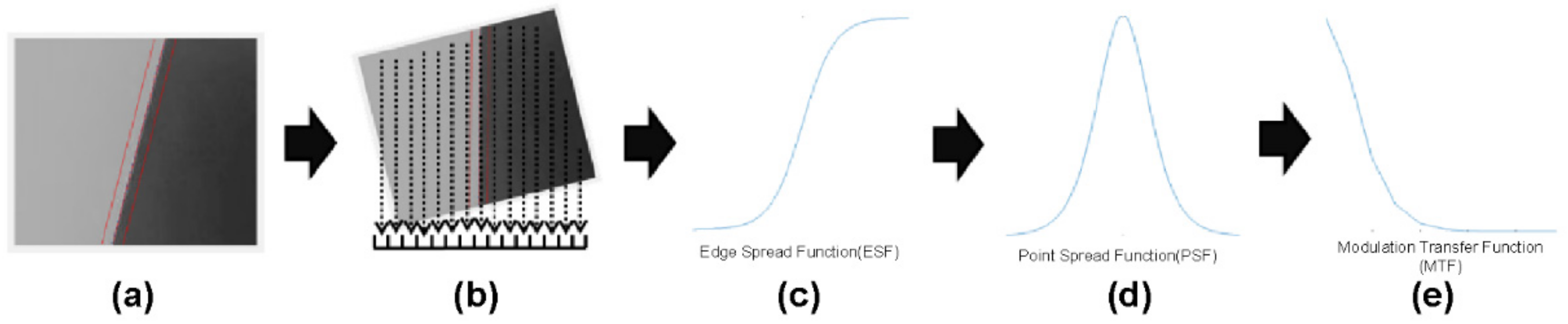
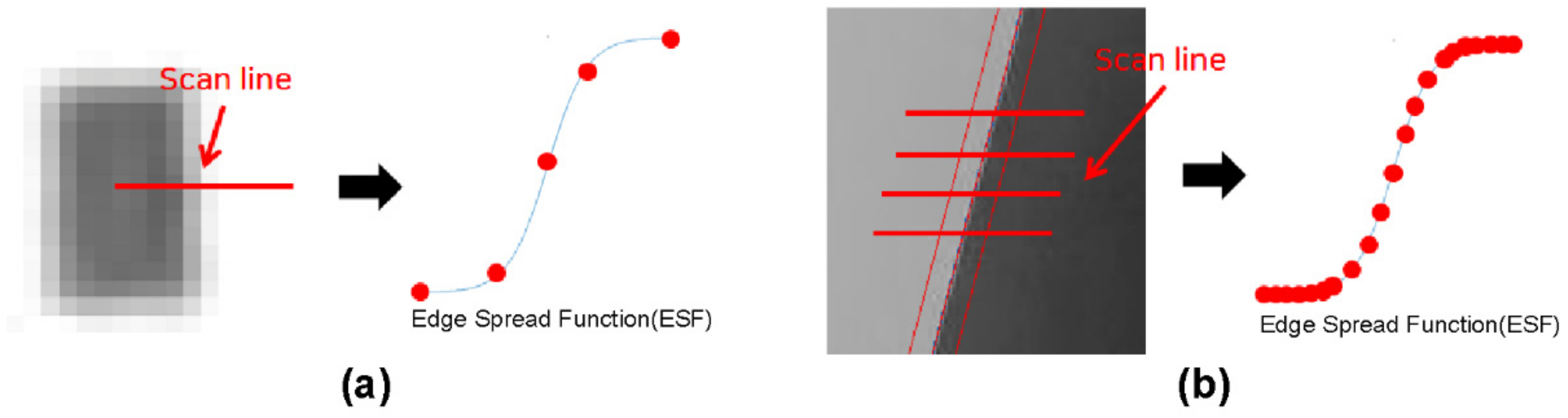
2.3. MTF Analysis Using the Slanted Edge Target

Figure 5a represents the slanted edge target and the boundary of the target is emphasized with a red dotted line. Figure 5b is the content of extracting DN from the target, and the black dotted line means extracting the DN value at the corresponding location. Figure 5c is the ESF graph generated from the extracted DN, Figure 5d is the PSF graph, and Figure 5e is the finally generated MTF graph.

The first step of the MTF analysis involves using the slanted edge target to find the boundary that is useful for analysis from the slanted edge target, as illustrated in Figure 5a. To find the boundary, a sufficient number of DNs is determined to produce the edge-spread function (ESF) and point-spread function (PSF) graphs stably. If too many DNs are extracted and analyzed, the image noise affects the MTF analysis. Sixteen DNs are typically used, but fifteen to sixteen DNs were used in this study.

In the second step, the mean of the DNs extracted from each line, as illustrated in Figure 5b, is calculated to generate the ESF illustrated in Figure 5c. Unlike the edge target, which is arrayed perpendicularly, the slanted edge target has slanted boundaries and different pixel array angles; hence, the mean DNs calculated from each line obtains the ESF without aliasing.

The most important step in an MTF analysis is detecting the boundary of the slanted edge target and extracting the DNs. If the perpendicular edge target is used, a few DNs are generated, as illustrated in Figure 6a. Figure 6b, however, shows that, if the slanted edge target is used to extract the DNs, multiple scan lines can be used, which makes it possible to extract and analyze an appropriate number of DNs across the boundary. In the case of a vertical edge target, the same set of DN values is generated at any location. However, in the case of a slanted edge target, a set of DN values is generated at different locations; thus, performing the MTF analysis is possible by extracting appropriate DN values across the entire boundary. The slanted edge target has an advantage as it obtains the ESF without aliasing from UAV images using the non-metric digital camera, and it enables a more accurate MTF analysis [20]. In the third step, the PSF graph is generated after the ESF graph is generated and differentiated, as illustrated in Figure 5d. Fitting the graph with the Gaussian function while producing the PSF graph reduces the effect of noise on the MTF value. Finally, the Fourier transform is used to generate the MTF graph from the PSF graph, as illustrated in Figure 5e.

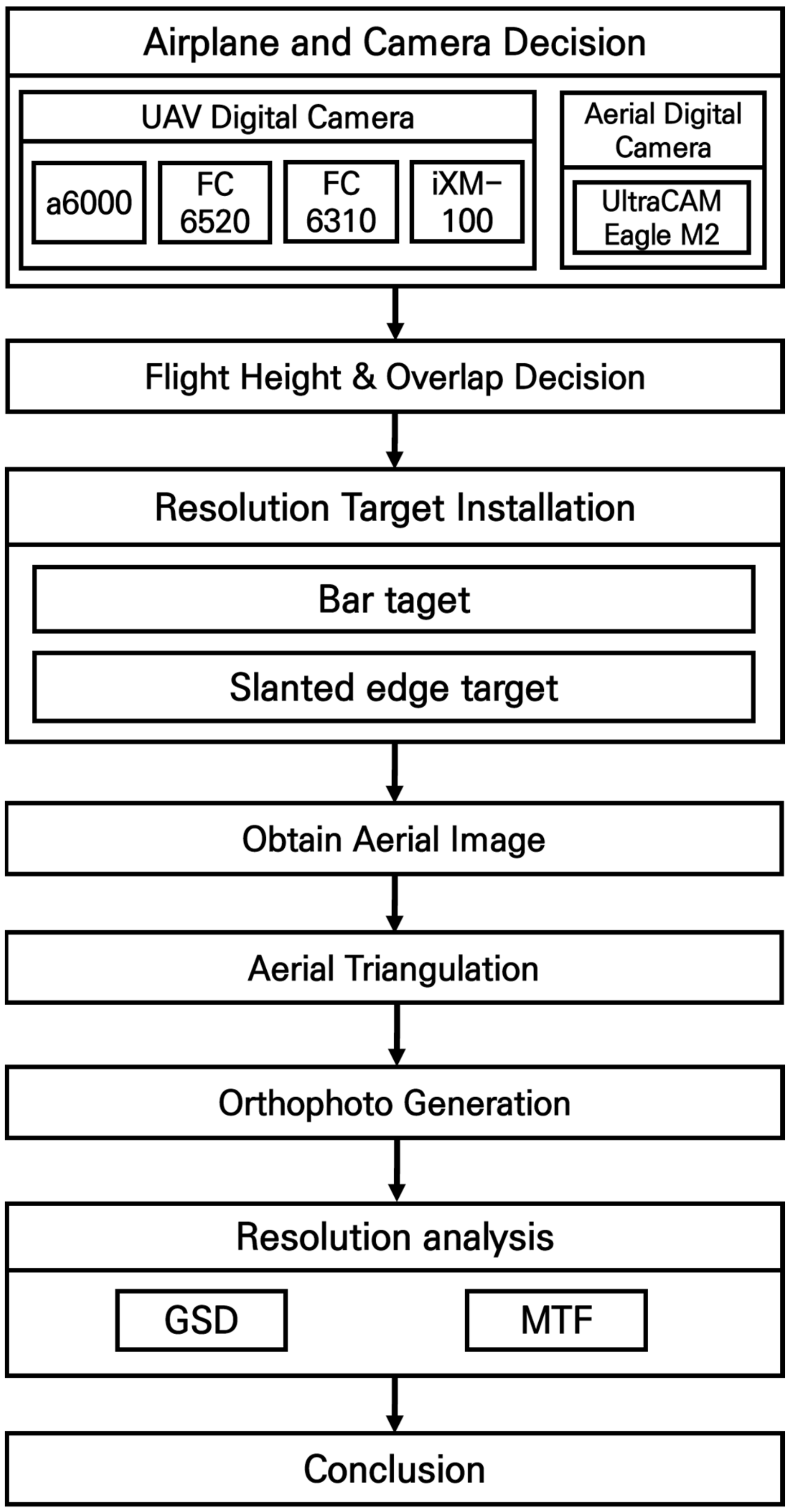
3. Materials and Methods

3.1. Specifications of Resolution Targets

3.1.1. Bar Target

The bar target in this study was developed based on the USAF 1951 test pattern, which is a resolution target used by the US Air Force to test the quality of sensors installed on UAVs, night goggles, and other image devices [21]. The USAF 1951 test pattern consists of 3 bars, and the distance between consecutive bars is fixed as a scale factor. Considering the characteristics of the unmanned aerial image, which has a higher resolution than the manned aerial image, in this study, the size of the bar pattern was successively reduced in 11 steps, as shown in Figure 7. The size was reduced by $1/\sqrt[6]{2}$ (approximately 12%) times in each step; thus, Bar 11 was 15.75 cm wide and 3.15 cm long. Therefore, the shape of a small bar can be visually identified in the image because a high-resolution sensor is mounted [21].

3.1.2. Slanted Edge Target

The image quality verification method using a slanted edge target has been widely used over the past 10 years. It has been adopted by several international standards, including the International Organization for Standardization (ISO). As shown in Figure 8, the angle of the slanted edge of the target was designed to be inclined at 5°, as stipulated in ISO 12233 [22]. In addition, the contrast between the black and white parts of the slanted edge target must be at least 40:1 in ISO 12233. However, the recently revised black and white contrast ratio is as 4:1 [22].

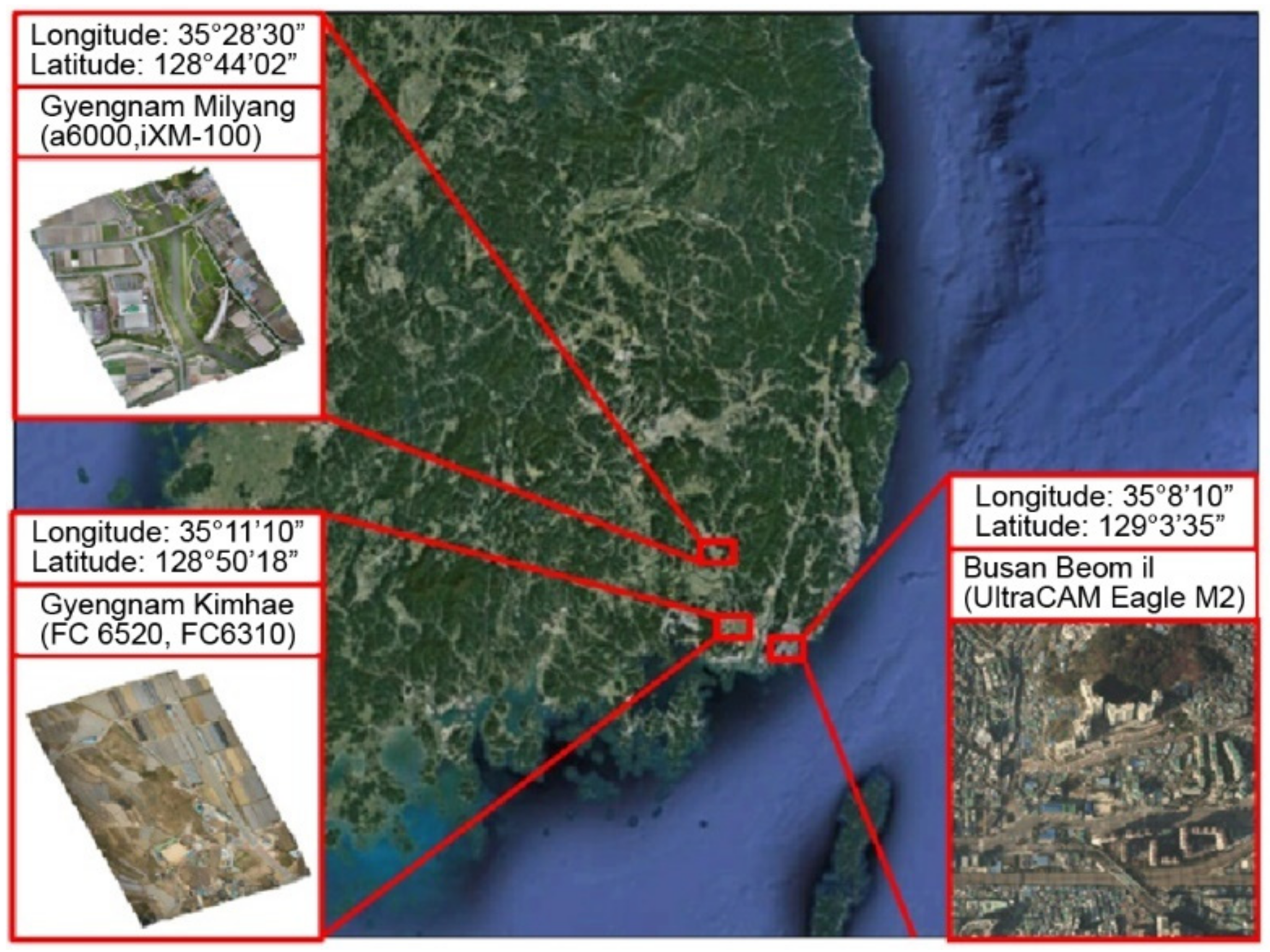
3.2. Resolution Target Installation

A resolution target was used for the UAV photogrammetry to improve the portability, ease of conducting the spatial resolution analysis of UAV photos, and outcomes, and work efficiency. The bar target was divided into 11 sizes; the largest bar was Size 1 (50 cm × 10 cm; width × height), and the size was reduced by $1\sqrt[6]{2}$ (about 12%) at every step to the smallest bar of Size 11 (15.75 cm × 3.15 cm; width × height). The slanted edge target was 60 cm × 130 cm (width × height), and the edge at the center was placed at 5°.

Three locations were selected for the UAV imaging: Miryang, Gyeongsangnam-do; Gimhae, Gyeongsangnam-do; and Beomil-dong, Busan. In Miryang, Gyeongsangnam-do, the a6000 and iXM-100 sensors were used for imaging; in Gimhae, Gyeongsangnam-do, the FC 6250 and FC 6310 sensors were used; and in Beomil-dong, Busan, the UltraCAM Eagle M2 manned aircraft sensor was used. Figure 9 shows the longitude, altitude, and coordinates of the three locations and the camera sensors used for imaging.

3.3. Image Acquisition and Processing

Table 1. Specifications of the UAVs, their cameras, and the manned aircraft sensor [23,24,25,26,27].

UAV Model	FireFLY 6 PRO	Inspire 2	Phantom Pro 4	Matrice 600	Manned Aircraft
Appearance
Camera model	a6000	FC 6520	FC 6310	iXM-100	UltraCAM Eagle M2
Focal length	20 mm	15 mm	8.8 mm	35 mm	100 mm
Pixel size	4 × 4 µm	3.28 × 3.28 µm	2.41 × 2.41 µm	3.76 × 3.76 µm	6 × 6 µm
CCD sensor size	6000 × 4000 (24 MP)	5280 × 3956 (21 MP)	5472 × 3648 (20 MP)	11,664 × 8750 (100 MP)	17,310 × 11,310 (193 MP)

lists the UAVs used to acquire the study data; these were: FireFly 6 pro (fixed-wing), Inspire 2, Phantom pro 4, and Matrice 600 (rotary-wing). The table also lists the specifications of the UltraCAM Eagle M2 manned aircraft sensor. The resolution of the camera in each UAV is also listed. In terms of the focal length, pixel size, and CCD sensor size, the iXM-100 sensor included in Matrice 600 had the best performance, followed by the a6000 sensor included in FireFLY 6 PRO, the FC 6520 sensor included in Inspire2, and the FC 6310 sensor included in Phantom pro 4. All unmanned aerial cameras were automatically set to capture the set shot-routed images.

To analyze the effects of flight height, camera performance, and imaging conditions on the quality of the UAV photos and outcomes, we designed the flight parameters as illustrated in

Table 2. Flight parameters used for analyzing UAV images.

Camera Model	Flight Height	Overlap	Area	Number of Images	Wind Velocity	Flight Date
a6000	150 m	P = 60%	720 m2	451	0.9 m/s	19 April 2011
		Q = 75%
FC 6520	150 m	P = 60%	422 m2	371	1.9 m/s	18 May 2022
		Q = 70%
FC 6310	80 m	P = 60%	894 m2	632	1.9 m/s	18 May 2022
		Q = 70%
	100 m	P = 60%	894 m2	556	1.9 m/s	18 May 2022
		Q = 70%
	150 m	P = 60%	894 m2	422	1.9 m/s	18 May 2022
		Q = 70%
iXM-100	150 m	P = 60%	462 m2	231	1.3 m/s	19 March 2028
		Q = 70%
	200 m	P = 60%	462 m2	115	1.3 m/s	19 March 2028
		Q = 70%
	400 m	P = 60%	462 m2	52	1.3 m/s	19 March 2028
		Q = 70%

. The term “overlap” refers to the degree of route overlap that occurred while capturing the UAV images. In overlap, P is the degree of overlap in the vertical direction of the photograph, and Q is the degree of overlap in the horizontal direction.

Metashape (v1.8.2, Agisoft, St. Petersburg, Russia) was used to calculate the results, and all parameters within the software were set to be the same.

4. Results

Based on the resolution target, we analyzed the quality of the images obtained by the UAVs and the manned aircraft. The results were divided into the outcomes of the GSD and MTF analyses as follows:

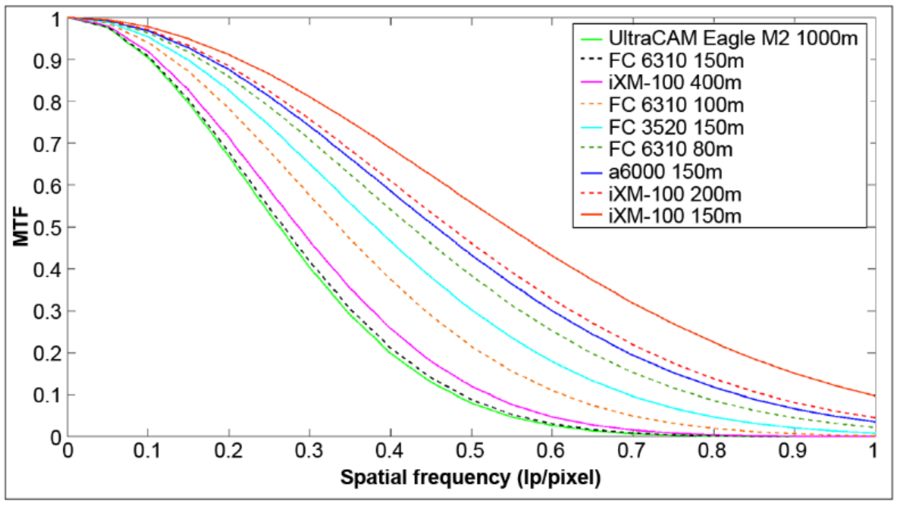
• To analyze the effect of camera performance on the quality of the UAV’s photos and outcomes, we set the flight height to be almost identical at 150 m, and the overlap at P = 60% and at Q = 70–75%. To compare the camera performance, we indicated the name of each camera model.
• Using the FC 6310 and iXM-100 sensors, we captured the images at different heights to analyze the effect of flight height on the quality of the UAV’s images and outcomes.
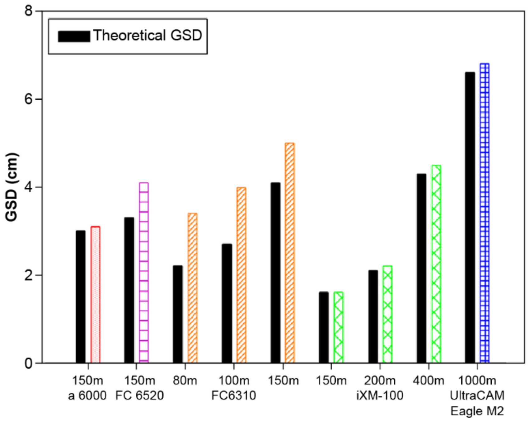
• The GSD and MTF of the manned aircraft images from the UltraCAM Eagle M2 sensor and of the UAV images from the four sensor types were analyzed and compared.

4.1. GSD Analysis

Table 3. GSD analysis results using bar target.

Camera Model	Flight Height	Bar Target	Theoretical GSD	Measured GSD
a6000	150 m		3.0 cm	3.1 cm
FC 6520	150 m		3.3 cm	4.1 cm
FC 6310	80 m		2.2 cm	3.4 cm
	100 m		2.7 cm	4.0 cm
	150 m		4.1 cm	5.0 cm
iXM-100	150 m		1.6 cm	1.6 cm
	200 m		2.1 cm	2.2 cm
	400 m		4.3 cm	4.5 cm
UltraCAM Eagle M2	1000 m		6.6 cm	6.8 cm

presents the results of the GSD analysis using the bar target. The flight height, camera focal length, and pixel size were used to calculate the theoretical GSD, which was compared with the measured GSD. Theoretical GSD can be calculated by multiplying the camera’s one-pixel size by the flight altitude and dividing by the focal length. In this context, the measured GSD deviates from the theoretical GSD, owing to errors in the correction values of the camera, the atmospheric conditions during image capture, the unmanned aerial vehicle’s dynamics, GPS error values, and other factors.

Figure 10 is a graph of the GSD results analyzed using bar targets for flight height. For FC 6310 sensors, the GSDs were 3.4 cm (80 m in height), 4.0 cm (100 m in height), and 5.0 cm (150 m in height) as the flight height increased, resulting in poor image quality. The GSDs for iXM-100 sensors decreased to 1.6 cm (150 m in height), 2.2 cm (200 m in height), and 4.5 cm (400 m in height) as the flight height increased. In addition, the GSD for the iXM-100 sensors, which showed the best performance at the same flight height of 150 m, was the best, with a value of 1.6 cm. Subsequently, the GSD values were 3.1 cm for the a6000 sensor, 4.1 cm for the FC 6520 sensor, and 5.0 cm for the FC 6310 sensor.

Figure 11 displays a graph of the theoretical and measured GSDs using the bar target. The GSDs of the FC 6520 and FC 6310 sensors differed by 18–35% from the theoretical GSD. The GSDs of the iXM-100, a6000, and UltraCAM Eagle M2 sensors, however, only differed slightly, by 0–5%, from their theoretical values. These results suggest that the FC 6520 and FC 6310 sensors were more affected than the other sensors by the factors that reduced the image quality during UAV image capturing. Hence, sensors that differed considerably from the theoretical GSD should be avoided or carefully tested.

4.2. MTF Analysis

In

Table 4. MTF analysis results using slanted edge target.

Camera Model	Flight Height	Slanted Edge Target	${\mathit{\sigma }}_{\mathit{M}\mathit{T}\mathit{F}}$	${\mathit{M}\mathit{T}\mathit{F}}_{50}$	${\mathit{M}\mathit{T}\mathit{F}}_{20}$
a6000	150 m		0.401	0.456	0.694
FC 6520	150 m		0.511	0.381	0.582
FC 6310	80 m		0.443	0.426	0.648
	100 m		0.522	0.336	0.513
	150 m		0.694	0.268	0.408
iXM-100	150 m		0.331	0.545	0.831
	200 m		0.395	0.474	0.722
	400 m		0.635	0.286	0.437
UltraCAM Eagle M2	1000 m		0.715	0.263	0.399

, ${\sigma }_{MTF}$ denotes the standard deviation of the MTF; the smaller the value of ${\sigma }_{MTF}$, the clearer the image. ${MTF}_{50}$ and ${MTF}_{20}$ were also calculated and compared. Considering the ${\sigma }_{MTF}$, the image quality worsened as the flight height increased in the MTF analysis, similar to those in the GSD, ground resolved distance (GRD), and edge response analyses.

As shown in Figure 12, the iXM-100 sensor maintained a high MTF value as the spatial frequency increased to a height of 150 m and showed significantly better MTF results than those for the other camera sensors. The ${\sigma }_{MTF}$ value for the iXM-100 sensor was the lowest at 0.331 (smaller the ${\sigma }_{MTF}$ value, better is the image quality). The image quality worsened from top to bottom in the order of the MTF curves of the sensors presented in Figure 12. Specifically, the iXM-100 sensor exhibited the best results at a height of 150 m with ${\sigma }_{MTF}$ = 0.331, ${MTF}_{50}$ = 0.545 lp/pixel, and ${MTF}_{20}$ = 0.831 lp/pixel. The UltraCAM Eagle M2 manned aircraft sensor exhibited the worst results, with ${\sigma }_{MTF}$ = 0.715, ${MTF}_{50}$ = 0.263 lp/pixel, and ${MTF}_{20}$ = 0.399 lp/pixel. At the same height of 150 m, the boundary of the black and white lp of 10 cm width began to blur from the GSD values of 3.31 cm for the iXM-100 sensor, 4.58 cm for the a6000 sensor, 3.75 cm for the FC 6520 sensor, and 2.65 cm for the FC 6310 sensor. The boundary of the black and white lp that was 10 cm in width was no longer identifiable above the values of 8.31 cm, 6.98 cm, 5.72 cm, and 4.04 cm for the iXM-100, a6000, FC 6520, and FC 6310 sensors, respectively. Moreover, the boundary of the black and white lp that was 10 cm in width started to blur from the GSD value of 2.63 cm for the UltraCAM Eagle M2 sensor, which exhibited the worst performance, and was no longer identifiable above 3.99 cm.

5. Conclusions

In this study, we acquired images from four types of UAVs and one type of manned aircraft to investigate the need for MTF analysis in UAV image quality assessment. We also examined the impact of shooting altitude and sensor performance on the quality of unmanned aerial images. An MTF analysis was conducted using a slanted edge target, while the GSD analysis was performed using a bar target.

First, the trend in ${\sigma }_{MTF}$ indicated that the image quality worsened as the flight height increased in both the MTF and GSD analyses. However, the ${\sigma }_{MTF}$ values were low for the FC 6520 and FC 6310 sensors, resulting in a slight blurring of the white object. The MTF analysis evaluates both image resolution and contrast; hence, slight blurring has a considerable effect on ${\sigma }_{MTF}$. However, the MTF analysis of the corresponding bar was not possible owing to contrast reduction of the bar target for which the visual resolution analysis was possible. The smallest bar that can be recognized as the bar target, which can be analyzed by visual resolution, determines the GSD of the corresponding image. For example, the FC 6310 sensor, at a shooting altitude of 150m, can analyze up to Bar 5, which is 6.3cm in size due to reduced contrast ratio. However, the GSD results analyzed using Bars 1–5 showed a 5cm result. Similarly, the iXM-100 sensor, at a 400m shooting altitude, can analyze up to Bar 6, which is 5.6cm in size due to reduced contrast ratio. However, the analyzed GSD result was 4.5cm. Therefore, the MTF, which can analyze both the degree of contrast and resolution of the image, was required to verify the quality of the unmanned aerial image, which experienced a deterioration in its quality owing to various factors, such as weather conditions, the use of non-surveying cameras, and low-cost navigation devices. Thus, the MTF analysis was proven to be a more objective and reliable method of analysis than the GSD analysis.

Secondly, we observed a decline in image quality for both the FC 6310 and iXM-100 sensors as shooting altitude increased. Furthermore, when comparing images captured by these sensors at the same altitude of 150 m, it was evident that the GSD and MTF values varied based on the sensor’s performance. Consequently, we confirmed that both shooting altitude and sensor performance significantly impact the image quality of UAV images.

Third, despite the UltraCAM Eagle M2 manned aircraft sensor exhibiting the poorest image quality, the results from the FC 6310 sensor were nearly identical at a height of 150 m compared to those from the UltraCAM Eagle M2 sensor. These observations suggest that obtaining high-quality UAV images during UAV photogrammetry is contingent upon the operator accurately determining appropriate camera-sensor parameters, overlapping, and UAV performance before capturing the images, regardless of the number of UAV sensors used.

In this study, we confirmed the necessity of both MTF analysis and GSD analysis for assessing image quality. This was achieved by conducting analyses at various research sites, adjusting the flight height, and using different mounted sensors, which exert the most significant influence on image quality. In future studies, if a test bed with a permanent UAV photogrammetry resolution target can be constructed to analyze the quality of the image under the same conditions, it will be possible to analyze it more quantitatively and objectively, and to accumulate data.

As a result of the analysis, it was determined that MTF analysis, which can analyze the resolution and contrast of images simultaneously, rather than GSD analysis, was a more objective and reliable method. It was found that high-quality unmanned aerial images could be obtained only when workers properly judge the performance of camera sensors, redundancy, and the aircraft’s performance.

References

1. Masita, K.; Hasan, A.; Shongwe, T. Defects Detection on 110 MW AC Wind Farm’s Turbine Generator Blades Using Drone-Based Laser and RGB Images with Res-CNN3 Detector. Appl. Sci. 2023, 13, 13046. [Google Scholar] [CrossRef]
2. Liu, Y.; Zhou, T.; Xu, J.; Hong, Y.; Pu, Q.; Wen, X. Rotating Target Detection Method of Concrete Bridge Crack Based on YOLO v5. Appl. Sci. 2023, 13, 11118. [Google Scholar] [CrossRef]
3. Lu, L.; Dai, F. Accurate road user localization in aerial images captured by unmanned aerial vehicles. Autom. Constr. 2024, 158, 105257. [Google Scholar] [CrossRef]
4. Ke, R.; Li, Z.; Tang, J.; Pan, Z.; Wang, Y. Real-Time Traffic Flow Parameter Estimation from UAV Video Based on Ensemble Classifier and Optical Flow. In IEEE Transactions on Intelligent Transportation Systems; IEEE: Piscataway, NJ, USA, 2018; pp. 54–64. [Google Scholar] [CrossRef]
5. Zhao, Y.; Zhou, L.; Wang, X.; Wang, F.; Shi, G. Highway Crack Detection and Classification Using UAV Remote Sensing Images Based on CrackNet and CrackClassification. Appl. Sci. 2023, 13, 7269. [Google Scholar] [CrossRef]
6. Ercolini, L.; Grossi, N.; Silvestri, N. A Simple Method to Estimate Weed Control Threshold by Using RGB Images from Drones. Appl. Sci. 2022, 12, 11935. [Google Scholar] [CrossRef]
7. Logan, R.D.; Torrey, M.A.; Feijó-Lima, R.; Colman, B.P.; Valett, H.M.; Shaw, J.A. UAV-Based Hyperspectral Imaging for River Algae Pigment Estimation. Remote Sens. 2023, 15, 3148. [Google Scholar] [CrossRef]
8. Rajeena, F.P.P.; Ismail, W.N.; Ali, M.A.S. A Metaheuristic Harris Hawks Optimization Algorithm for Weed Detection Using Drone Images. Appl. Sci. 2023, 13, 7083. [Google Scholar] [CrossRef]
9. Diruit, W.; Le Bris, A.; Bajjouk, T.; Richier, S.; Helias, M.; Burel, T.; Lennon, M.; Guyot, A.; Ar Gall, E. Seaweed Habitats on the Shore: Characterization through Hyperspectral UAV Imagery and Field Sampling. Remote Sens. 2022, 14, 3124. [Google Scholar] [CrossRef]
10. Fabris, M.; Balin, M.; Monego, M. High-Resolution Real-Time Coastline Detection Using GNSS RTK, Optical, and Thermal SfM Photogrammetric Data in the Po River Delta, Italy. Remote Sens. 2023, 15, 5354. [Google Scholar] [CrossRef]
11. Domingo, D.; Gómez, C.; Mauro, F.; Houdas, H.; Sangüesa-Barreda, G.; Rodríguez-Puerta, F. Canopy Structural Changes in Black Pine Trees Affected by Pine Processionary Moth Using Drone-Derived Data. Drones 2024, 8, 75. [Google Scholar] [CrossRef]
12. Sung, S.M. A Study on Spatial Resolution Analysis Methods of UAV Images. Ph.D. Dissertation, Dong-A University, Busan, Korea, 20 August 2019. [Google Scholar]
13. Baer, L.R. Circular-edge spatial frequency response test. In Proceedings Society of Photo-Optical Instrumentation Engineers, Image Quality and System Performance, San Jose, CA, USA, 18 December 2003; Yoichi Miyake, D., Rene, R., Eds.; SPIE: Bellingham, WA, USA, 2003. [Google Scholar]
14. Wang, T.; Li, S.; Li, X. An automatic MTF measurement method for remote sensing cameras. In Proceedings of the 2nd IEEE International Conference on Computer Science and Information Technology, Beijing, China, 8–11 August 2009; pp. 245–248. [Google Scholar]
15. Sieberth, T.; Wackrow, R.; Chandler, J.H. Automatic detection of blurred images in UAV image sets. ISPRS J. Photogramm. Remote Sens. 2016, 122, 1–16. [Google Scholar] [CrossRef]
16. Orych, A. Review of methods for determining the spatial resolution of UAV sensors. Int. Arch. Photogramm. Remote Sens. Spat. Inf. Sci. ISPRS Arch. 2015, XL-1/W4, 391–395. [Google Scholar] [CrossRef]
17. Lee, T.Y. Spatial Resolution Analysis of Aerial Digital Camera. Ph.D. Dissertation, Dong-A University, Busan, Korea, 2012; 50p. (In Korean with English abstract). [Google Scholar]
18. Neumann, A. Verfahren zur Auflösungsmessung Digitaler Kameras. Masters’s Thesis, University of Applied Sciences, Cologne, Germany, 2003; 70p. [Google Scholar]
19. Pedrotti, F.L.; Pedrotti, L.M. Introduction to Optics, 3rd ed.; Cambridge University Press: Cambridge, UK, 2017. [Google Scholar]
20. Crespi, M.; De Vendictis, L. A Procedure for High Resolution Satellite Imagery Quality Assessment. Sensors 2009, 9, 3289–3313. [Google Scholar] [CrossRef] [PubMed]
21. Pinkus, A.; Task, H. Measuring Observers’ Visual Acuity Through Night Vision Goggles; Defense Technical Information Center: Fort Belvoir, VA, USA, 1998. [Google Scholar]
22. ISO 12233:2000(E); Photography–Electronic Still-Picture Cameras—Resolution Measurements. ISO: Geneve, Switzerland, 2000.
23. Geo-Matching. Available online: https://geo-matching.com/uas-for-mapping-and-3d-modelling/firefly6-pro (accessed on 20 January 2024).
24. Inspire 2. Available online: https://www.dji.com/inspire-2 (accessed on 20 January 2024).
25. Support for Phantom 4 Pro. Available online: https://www.dji.com/phantom-4-pro (accessed on 20 January 2024).
26. MATRICE 600PRO. Available online: https://www.dji.com/matrice600-pro (accessed on 20 January 2024).
27. EagleM2. Available online: https://www.vexcel-imaging.com/EagleM2 (accessed on 20 January 2024).
Figure 1. Research flow chart illustrating the experimental setup and methodology.
Applsci 14 02154 g001
Figure 2. Concept of modulation value analysis.
Applsci 14 02154 g002
Figure 3. DNs extracted from an image of a pair of black and white lines.
Applsci 14 02154 g003
Figure 4. MTF graph for explaining MTF20 and MTF50 (iXM-100 400 m).
Applsci 14 02154 g004
Figure 5. MTF analysis step using slanted edge target. (a) represents the slanted edge target and the boundary of the target is emphasized with a red dotted line. (b) is the content of extracting DN from the target, and the black dotted line means extracting the DN value at the corresponding location. (c) is the ESF graph generated from the extracted DN, (d) is the PSF graph, and (e) is the finally generated MTF graph.
Applsci 14 02154 g005
Figure 6. ESF graph of edge target (a) and slanted edge target (b).
Applsci 14 02154 g006
Figure 7. Specification of simple resolution bar target for UAV photogrammetry.
Applsci 14 02154 g007
Figure 8. Specifications of the slanted edge target for UAV photogrammetry.
Applsci 14 02154 g008
Figure 9. Map of the location of the study area.
Applsci 14 02154 g009
Figure 10. Comparison of the ground sample distance (GSD) analysis results obtained using the bar target.
Applsci 14 02154 g010
Figure 11. Comparison between the theoretical GSD and measured GSD using bar target.
Applsci 14 02154 g011
Figure 12. Comparison of the MTF curves obtained from cameras using slanted edge target.
Applsci 14 02154 g012