Improved SE-ResNet Acoustic–Vibration Fusion for Rolling Bearing Composite Fault Diagnosis

Featured Application

The fault diagnosis method proposed in this paper can be applied to the diagnosis of bearings in machine tool spindle systems.

Abstract

An enhanced fault diagnosis approach for rolling bearings with composite faults using an optimized Squeeze and Excitation ResNet (SE-ResNet) model is proposed. This method integrates grid search (GS), support vector regression (SVR), ensemble empirical mode decomposition (EEMD), and low-rank multimodal fusion (LMF) to effectively handle the signals of acoustic–vibration fusion. By combining these techniques, the aim is to improve the accuracy and reliability of rolling bearing fault diagnosis. Firstly, improved EEMD combined with GS-SVR and a window function is used for rolling bearing vibration signal decomposition. Singular value methods are used to filter and reconstruct the results. Secondly, Markov transition fields (MTFs) are used to encode vibration signals into 2D images. LMF is used for the fusion of vibration and sound signals. An improved Squeeze and Excitation ResNet50 network is proposed for feature identification and classification of rolling bearing composite fault data. Finally, the method undergoes rigorous testing and evaluation using rolling bearing data. The experimental outcomes demonstrate that, in comparison to traditional neural networks, the enhanced SE-ResNet, integrated with GS-SVR-EEMD and LMF, attains superior diagnostic accuracy. Additionally, the proposed approach can be effectively utilized for diagnosing rolling bearing composite faults.

1. Introduction

Bearings have widespread applications across various mechanical equipment fields. Ensuring their stable operation serves as a crucial prerequisite for the smooth functioning of such equipment [1]. The study of fault diagnosis methods has been a popular topic of research [2,3,4]. With the advent of the era of combining the machinery industry with big data, deep learning is presently one of the most intelligent features and cutting-edge research fields in fault diagnosis.

The heart of intelligent fault diagnosis lies in the efficient acquisition, transmission, processing, reformation, and utilization of diagnostic information [5,6,7]. In turn, it can achieve the ability to accurately perform feature recognition and prediction of diagnostic objects in a given environment. For instance, convolutional neural networks (CNNs), generative adversarial networks (GANs), recurrent neural networks (RNNs), and auto encoders have been developed for fault diagnosis applications. CNNs are primarily employed for grid-like structured data, including images and speech, whereas auto encoders are predominantly utilized for unsupervised learning tasks such as data dimensionality reduction and feature extraction [8,9,10]. Notably, CNNs have garnered significant research attention. Numerous scholars have utilized them in rolling bearing fault diagnosis, achieving remarkable results. Liang et al. [11] proposed a wavelet transform and improved RNN based on the new pooling layer for dimensionality reduction of the feature map. Singular value adaptive decomposition is used for feature extraction. This method was verified on two bearing datasets for feasibility and robustness. Tao et al. [12] proposed a combination of a GAN and short-time Fourier transform. The signal undergoes a transformation into a time–frequency map via the short-time Fourier transform (STFT), serving as the input for the classification GAN. Subsequently, the classification of bearings for fault diagnosis was achieved using the bearing dataset from Case Western Reserve University. Yang et al. [13] proposed a hybrid CNN model with good robustness. This method involves combining CNN with random forest. The CNN is employed to autonomously extract features from the grayscale map of the input signal. Subsequently, a random forest algorithm is applied for fault classification. The experimental outcomes demonstrated that the model attained a diagnostic accuracy of 99.548% on the high-speed bearing dataset provided by Case Western Reserve University. Chen et al. [14] utilized a continuous wavelet transform to convert the bearing vibration data into time–frequency maps. Advanced features are extracted by constructing a CNN with a square pooling structure. The extreme learning machine serves as a robust classifier. The dataset of motor bearings served to validate the effectiveness of the proposed method. Pham et al. [15] constructed a spectrogram from the raw data through the application of the short-time Fourier transform. Then, it was sent to the CNN for fault classification. High accuracy was achieved.

The above studies indicate that neural networks can be effectively integrated with other methods. Numerous scholars have conducted pertinent research exploring the integration of neural networks with other methodologies for fault diagnosis in distinct operational environments. This further enhances the application value of neural networks. Zhou et al. [16] integrated deep CNNs with gated recurrent units for bearing fault diagnosis. The raw signals, without preprocessing, are fed into the deep CNN, and its outputs are subsequently input to the GRU. This approach effectively diagnoses faults in rolling bearings. As another example, Lei et al. [17] introduced an intelligent bearing fault diagnosis method that combines adaptive variational mode decomposition (AVMD), a deep belief network (DBN) based on mode ordering, and an extreme learning machine (ELM). This method can adaptively decompose unsteady vibration signals into temporary frequency components, organize a set of effective frequency components, and facilitate online fault diagnosis. Additionally, Jin et al. [18] proposed an enhanced CNN-based fault diagnosis approach for rotating machinery. With a reduced number of parameters, it can swiftly and precisely identify fault types, thereby enhancing the efficiency of fault diagnosis. Khorram et al. [19] explored a deep learning approach for bearing fault diagnosis, incorporating a CNN and LSTM; however, their study was limited to a specific fault type. Similarly, Hoang et al. [20], making use of multi-sensor fusion, utilized deep neural networks for bearing fault diagnosis, but their research also focused on only a single fault type. The literature on composite fault diagnosis remains limited compared to individual fault diagnosis.

The majority of the aforementioned studies focus on single-fault scenarios. With the development and wide use of machinery industry, composite faults of rolling bearings appear frequently. Fan et al. [21] introduced an intelligent diagnosis model that combines a CNN with a support vector machine, successfully diagnosing various composite faults between rolling bearings and rotors. Their results demonstrated the model’s strong generalization capabilities in identifying different composite faults. Furthermore, An et al. [22] enhanced the LeNet network by designing the LeNet-F network specifically for composite fault diagnosis. This model, validated on the K210 development board, achieved a composite fault classification accuracy of 97.41%. Zhao et al. [23] proposed a method for composite fault diagnosis in rolling bearings that employs multi-scale fuzzy entropy feature fusion. This approach improves the discriminatory power of composite fault features compared to traditional methods that are limited to extracting single fault feature information. Cheng et al. [24] introduced the enhanced periodic mode decomposition (EPMD) method, the experimental results of which indicate as an effective tool for diagnosing composite faults in rolling bearings.

Through the analysis of existing literature, rolling bearings have been found to be widely utilized in various fields, such as machine tools, steel production, and electricity generation. They serve as crucial components of rotating machinery. Effective condition monitoring and fault diagnosis are essential for their maintenance. Accurate diagnosis of faults, particularly in their early stages, will contribute significantly to the stable operation of the equipment. Composite faults in bearings are more difficult to diagnose than individual faults. Limited research exists on the utilization of an acoustic–vibration combination for addressing composite fault problems. Some models have achieved high accuracy, but are complex. Some models are simpler, but have only achieved average accuracy. Deep learning methods for diagnosing composite faults often require deeper network structures. In this article, effective noise reduction processing is conducted before fault diagnosis. This ensures precision without adding undue complexity to the network. The key aspects of this paper are as follows: Firstly, an enhanced EEMD technique, incorporating GS-SVR alongside a window function, is introduced to reduce noise in rolling bearing vibration signals. Subsequently, MTFs are employed to transform one-dimensional signal data into two-dimensional images post-noise reduction. Next, a rolling bearing composite fault diagnosis approach that makes use of the SE attention mechanism and ResNet network is proposed. Lastly, comparative analysis with alternative network structures validates the stability of the enhanced SE-ResNet, satisfying the anticipated requirements for composite fault detection.

2. Methods

2.1. GS-SVR-EEMD with Window Function

Ensemble empirical modal decomposition aids signal analysis by adding white noise to the EMD approach. Its resistance to miscibility is improved. Support vector machine regression employs an SVM approximation function to establish a nonlinear mapping between the input vectors and the feature space. Subsequently, a linear regression analysis is conducted within the feature space to formulate the decision function. The SVM function expression is as follows:

$$f\left(x_i\right)={\omega }^T{x}_i+b,$$

(1)

To address the challenge of SVM regression fitting, Vapnik and his colleagues introduced an insensitive loss coefficient to the SVM, subsequently evolving it into the SVR method. The insensitivity loss factor $\epsilon$ is as follows:

$$L_{\epsilon }\left(f\left(x_i\right)-y_i\right)=\left\{\begin{array}{c}0,\hspace{1em}\hspace{1em}\hspace{1em}\hspace{1em}\hspace{1em}\left|f\left(x_i-y_i\right)\right|\le \epsilon \\ \left|f\left(x_i-y_i\right)\right|-\epsilon ,\hspace{1em}\hspace{1em}\hspace{1em}\hspace{1em}\mathrm{else}\end{array}\right.,$$

(2)

Based on the principle of structural risk minimization, the convex quadratic programming problem of linear regression is derived. Based on the difference in the degree of relaxation between the two sides of the spacer band, the relaxation variables ${\xi }_i$ and ${\widehat{\xi }}_i$ are introduced.

$$\underset{\omega ,b,\xi ,{\xi }_i}{\min }\frac{1}{2}‖{\omega }^2‖+C{\displaystyle \sum _{i=1}^N\left({\widehat{\xi }}_i+{\xi }_i\right)},$$

(3)

where C is the penalty factor. After a Lagrange transformation, this problem is transformed into a dyadic problem.

$$\max \mathrm{G}\left(\alpha \right)=-\frac{1}{2}{\displaystyle \sum _{i,j=1}^N\left({\alpha }_i-{\widehat{\alpha }}_i\right)}\left({\alpha }_j-\widehat{\alpha }\right)〈x_i,x_j〉-\epsilon {\displaystyle \sum _{i=1}^N\left({\alpha }_i+{\widehat{\alpha }}_i\right)}+{\displaystyle \sum _{i=1}^N{y}_i\left({\alpha }_i-{\widehat{\alpha }}_i\right)},$$

(4)

In nonlinear regression problems, a kernel function is utilized to transform the nonlinear data into a higher-dimensional feature space, within which linear regression is then performed. The regression function is given as follows:

$$f\left(x\right)={\displaystyle {\sum }_{i=1}^N\left({\alpha }_i-{\widehat{\alpha }}_i\right)}\mathsf{\Phi }\left(x_i\right)\mathsf{\Phi }\left(x\right)+b={\displaystyle {\sum }_{i=1}^N\left({\alpha }_i-{\widehat{\alpha }}_i\right)}k\left(x_i,x\right)+b,$$

(5)

The kernel function employed is a Gaussian kernel function, expressed as follows:

$$\mathrm{K}\left(x_i,x\right)=e^{-g{\left|x_i-x_j\right|}^2},$$

(6)

The GS algorithm is applied to optimize the penalty factor and the parameters of the kernel function in SVR. The details of the GS-SVR process are as follows:

(1)

Determine the range of the optimization search for GS.

(2)

Determine the step size. A grid is constructed based on the varying directions of growth for the parameters. The nodes within this grid represent the corresponding parameter sets.

(3)

Iterate over each parameter in the range to be searched and take a series of discrete values for each. Train the model by taking all combinations of the values for the parameters to be tested, respectively.

(4)

The parameters that give the best results in training the model are chosen as the optimal parameter set.

(5)

The optimal parameters obtained are substituted into the SVR model.

In the methodology proposed in this paper, the initial signal undergoes endpoint extension. Samples proximal to the endpoints are chosen to constitute the training set. Subsequently, the aforementioned GS-SVR is utilized for data prediction. Predicted values are used as new boundary points for continuous prediction extension to a set value.

The endpoint extension does not guarantee that the endpoints are extreme. Therefore, a rectangular window and the Hanning window, respectively, are used to window the delayed signal. EEMD decomposition is used after the endpoint extension. Valid IMFs are obtained after removing the delayed part.

The procedure for noise reduction in the original signal is outlined as follows:

(1)

The aforementioned GS-SVR-EEMD method, incorporating a window function, is employed to decompose the original signal, yielding a sequence of IMF components along with residual signals.

(2)

The correlation coefficient between each IMF component and the original signal is calculated.

(3)

At the first local maximum in the difference of the correlation coefficients, the preceding IMF component is eliminated.

(4)

Singular value decomposition noise reduction is conducted for the remaining IMF components.

(5)

The processed signal data is obtained by accumulating the IMF components after noise reduction.

2.2. Low-Rank Multimodal Fusion

The feature fusion of multiple modalities can obtain the correlation and complementary information between different modalities. The low-rank multimodal fusion method, introduced by Liu and his colleagues, is the multimodal fusion approach utilized in this paper [25]. The details are as follows.

The set of vectors representing the M modal coded messages is ${\left\{Z_m\right\}}_{m=1}^M$. The tensor is represented by extracting the outer product of multiple modal features from the input. Prior to the computation of the outer product, the vectors are appended to the rear of each modal feature. This is done to model the interactions between subsets of the modalities. The unimodal input tensor is

$$Z={\otimes }_{m=1}^M{Z}_m,Z_m\in R^{d_m},$$

(7)

where ${\otimes }_{m=1}^M$ is the outer product of the tensor. $Z_m$ represents the input representation resulting from the vector splicing operation. The input tensor is forwarded through the linear layer to produce a vector, as follows:

$$h=g\left(Z;W,b\right)=W\times Z+b,$$

(8)

where W is the weight tensor and b is the offset. Since Z is a tensor of order M, W is a tensor of order M + 1. The dimension is $d_1\times d_2\times \dots \times d_m\times d_h$. This method requires the creation of a high-dimensional tensor. Its dimension is ${\prod }_{m=1}^M{d}_m$. The number of parameters to be learned by W will then show exponential growth. Low-rank multimodal fusion decomposes the weight tensor into a modality-specific set of low-rank factors. This allows the high-dimensional tensor to be obtained non-explicitly and h to be computed. Let the weight tensor W be a set of d_h order-M tensors. For an order-M tensor ${\overline{W}}_k\in R^{d_1\times d_2\times \dots \times d_m},k=\mathrm{1,2},\dots ,d_h$, there exists an exact form of vector decomposition:

$${\overline{W}}_k={\displaystyle \sum _{i=1}^R{\otimes }_{m=1}^M}{w}_{m,k}^{\left(i\right)},w_{m,k}^{\left(i\right)}\in R^{d_m},$$

(9)

where R, which makes the decomposition valid and minimal, is the rank of the tensor. Give this value of R to r. r decomposition factors are used to reconstruct a low-rank version of ${\overline{W}}_k$. The new weight tensor is

$$W={\displaystyle \sum _{i=1}^r{\otimes }_{m=1}^M}{w}_m^{\left(i\right)},$$

(10)

After decomposing Z into ${\left\{Z_m\right\}}_{m=1}^M$, h can be derived as

$$h=\left({\displaystyle \sum _{i=1}^r{\otimes }_{m=1}^M}{w}_m^{\left(i\right)}\right)\times Z=\underset{m=1}{\overset{M}{\Lambda }}\left[{\displaystyle \sum _{i=1}^r{w}_m^{\left(i\right)}\times Z_m}\right],$$

(11)

where ${\Lambda }_{m=1}^M\left[·\right]$ is the product of tensors. $w_m^{\left(i\right)}$ is the i-th low-rank decomposition factor of mode M. The low-rank multimodal fusion structure is shown in Figure 1.

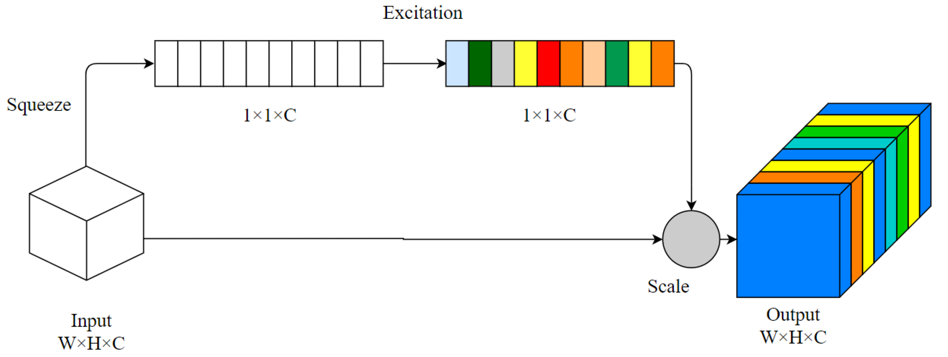
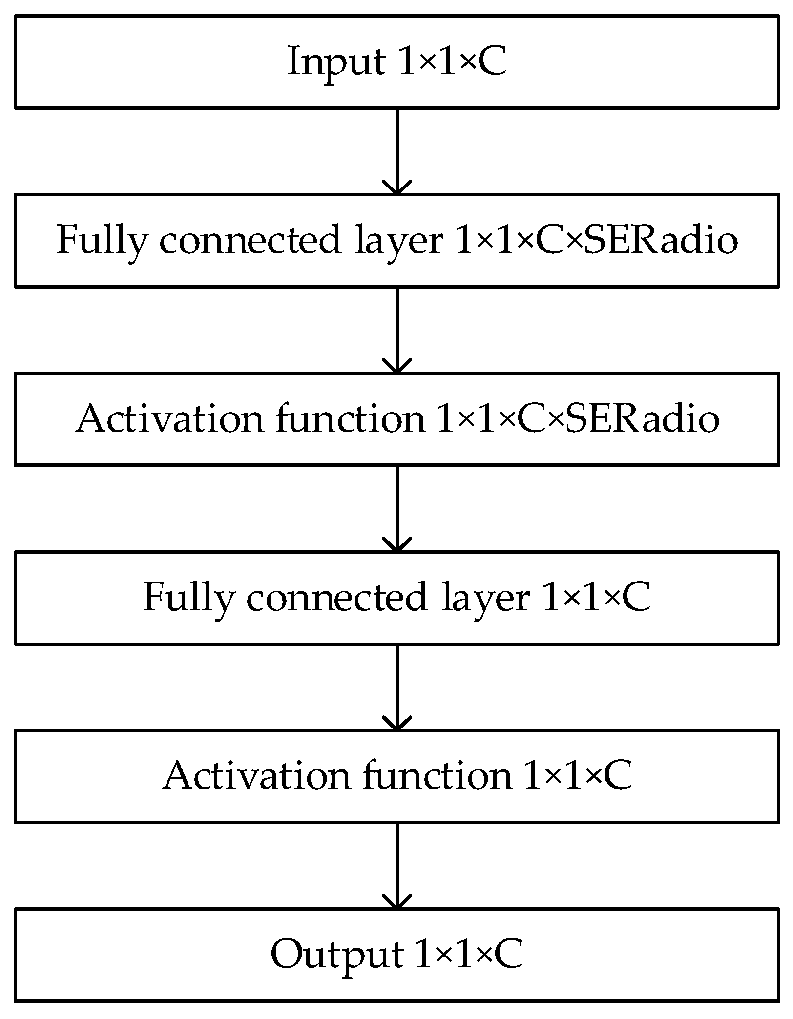
2.3. Improved SE-ResNet

The SE attention module is a representation of channel attention. It focuses on the problem of interdependence between model channels. The convolution operation first convolves each channel of the input, then sums the results of the convolution for each channel. This allows spatial features to be fused with channel features, resulting in a particularly mixed set of features. The SE module abstracts this confounding and allows the deep learning model to learn directly on the channel features. SE brings out the interdependencies between feature channels, obtaining the importance of each channel. Features on each channel are weighted, accentuating important features and suppressing secondary ones. The SE attention mechanism module can be easily ported to other network architectures. As depicted in Figure 2, the SE module has three main operations: compression, excitation, and scale. W stands for width, H stands for height, and C stands for channels.

Squeeze employs global pooling to condense the spatial characteristics of each channel into a singular global feature, effectively integrating the information from each channel feature. Subsequently, a fully connected (FC) layer is incorporated to assess the significance of each channel based on the compressed global features obtained. Figure 3 shows the excitation operation. The weight values for each channel, determined by the SE module, are individually multiplied with the matrix corresponding to the respective channel in the original feature map.

Microsoft Labs introduced ResNet in 2015. Currently, ResNet has gained widespread application in feature extraction across diverse fields. ResNet’s residual module can better utilize the shallow features of the data to obtain more critical features. In the task of feature recognition and classification, the residual module is used as the main feature extraction structure.

After several experimental comparisons, it was decided that the ResNet50 network and the SE attention module would be used in this paper, as shown in

Table 1. SE-ResNet50 network architecture.

Layer Name	Output Size	50-Layer
conv1	$112\times 112$	$7\times 7$, 64, stride2
conv2_x	$56\times 56$	$3\times 3$ max pool, stride2
		$\left[\begin{array}{c}\begin{array}{c}1\times 1,64\\ 3\times 3,64\\ 1\times 1,256\end{array}\\ fc,\left[\mathrm{16,256}\right]\end{array}\right]\times 3$
conv3_x	$28\times 28$	$\left[\begin{array}{c}\begin{array}{c}1\times 1,128\\ 3\times 3,128\\ 1\times 1,512\end{array}\\ fc,\left[\mathrm{32,512}\right]\end{array}\right]\times 4$
conv4_x	$14\times 14$	$\left[\begin{array}{c}\begin{array}{c}1\times 1,256\\ 3\times 3,256\\ 1\times 1,1024\end{array}\\ fc,\left[\mathrm{64,1024}\right]\end{array}\right]\times 6$
conv5_x	$7\times 7$	$\left[\begin{array}{c}\begin{array}{c}1\times 1,512\\ 3\times 3,512\\ 1\times 1,1048\end{array}\\ fc,\left[\mathrm{128,2048}\right]\end{array}\right]\times$ 3
	$1\times 1$	Average pool, 1000-d fc, softmax
FLOPs		$3.8 \times {10}^9$

:

3. Test Verification

3.1. Data Preprocessing

The experiment was performed on a QPZZ-II test rig, as depicted in Figure 4. The acoustic microphone and vibration sensor arrangement is shown in Figure 5. The bearings were mounted on the spindle. Two vibration sensors were placed vertically on the bearing housing to collect vibration data. Nine microphones were utilized for the measurement, with Microphone Number 0 positioned at the center to capture mono signals.

Four distinct test conditions were examined: outer race fault, inner race fault, mixed inner and outer ring failure, and normal state. The physical diagrams depicting the inner ring failure and outer ring failure are comprehensively outlined in Figure 6. The model number of the bearing was HRB N205EM. Specific parameters are detailed in

Table 2. Bearing configuration.

Pitch Diameter	Ball Diameter	Ball Number	Contact Angle
39 mm	7.5 mm	13	0°

.

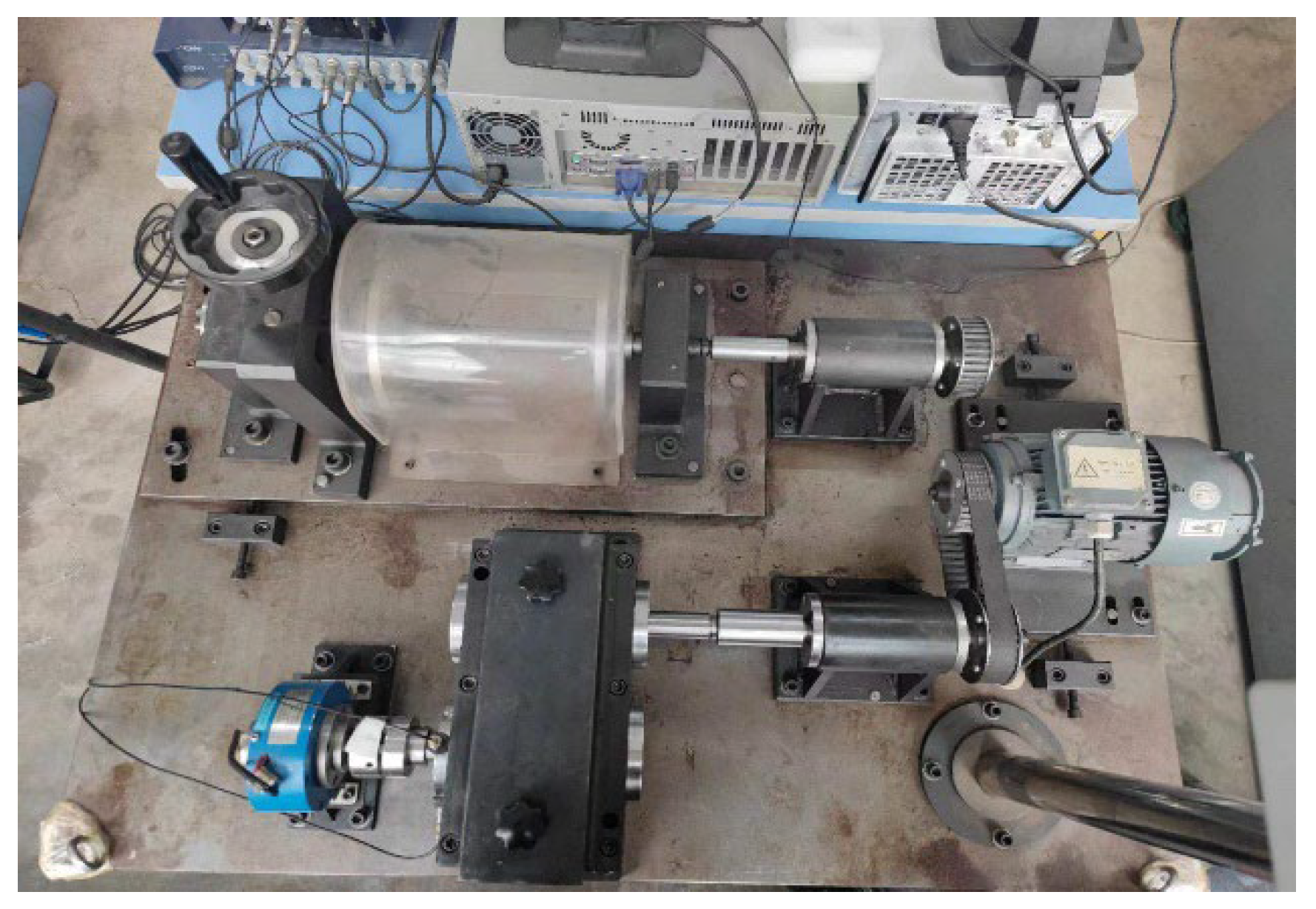
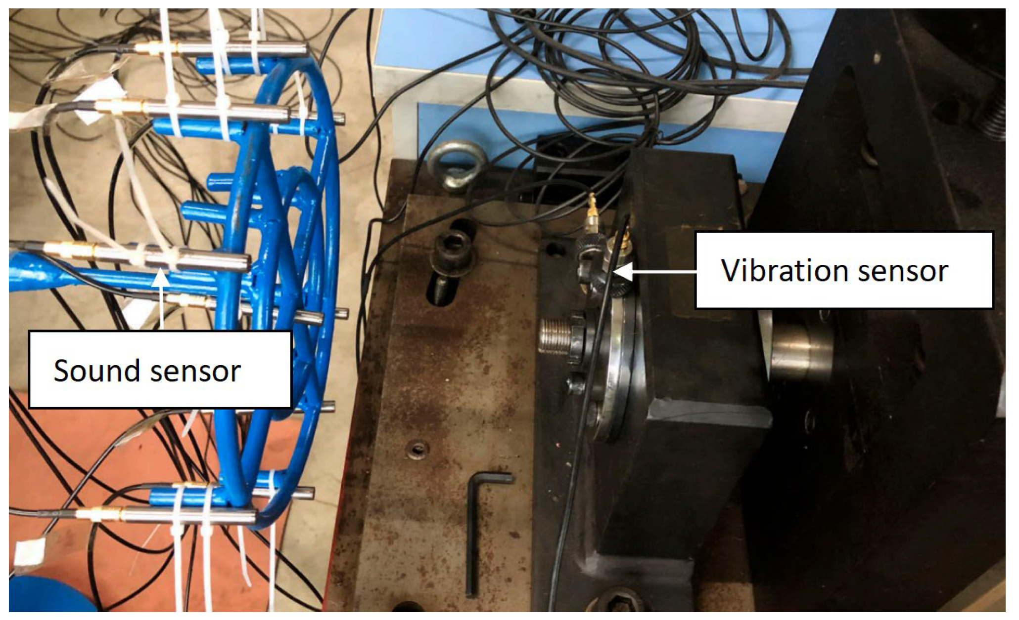
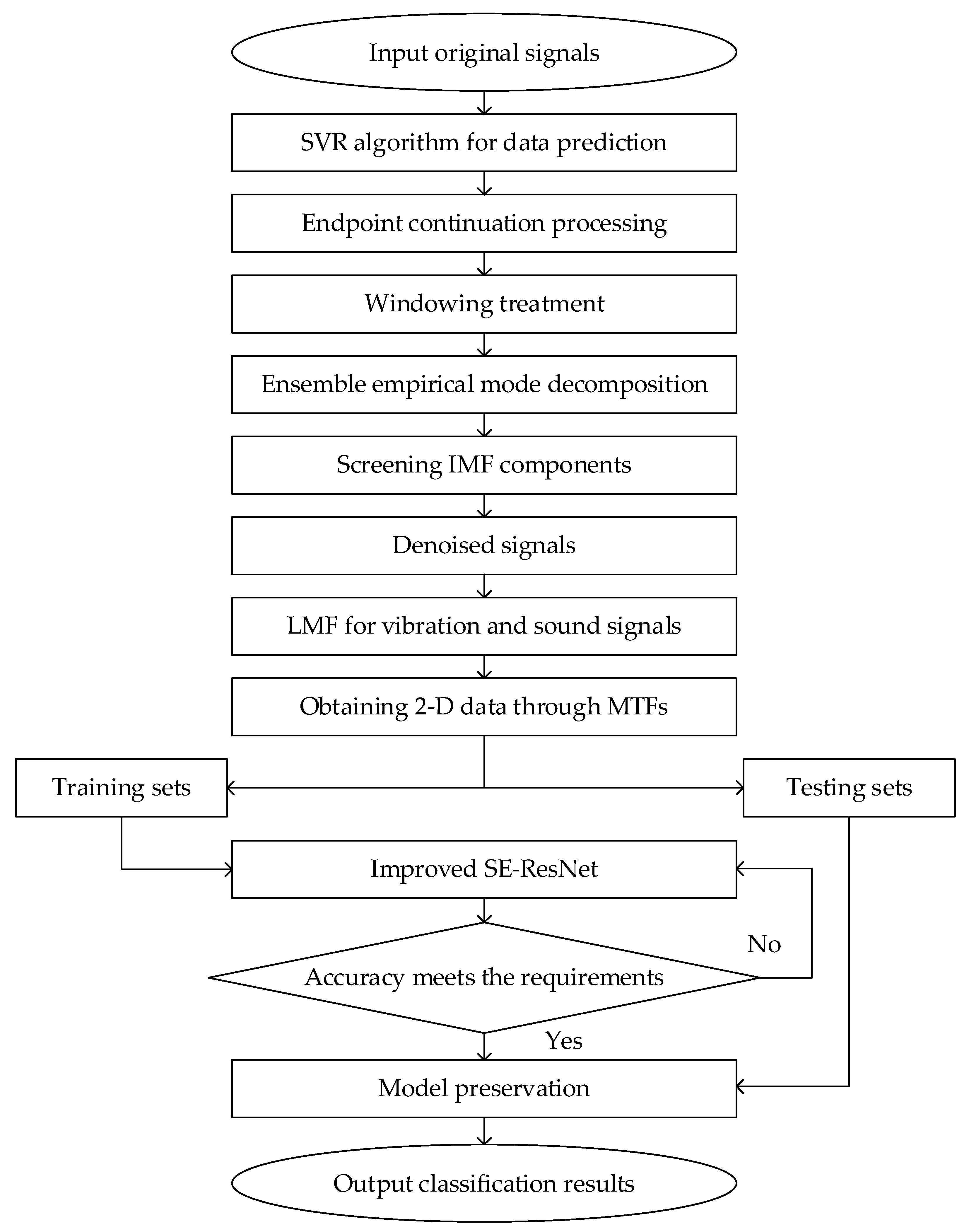
3.2. Experimental Method

The detailed experimental procedure is outlined below:

(1)

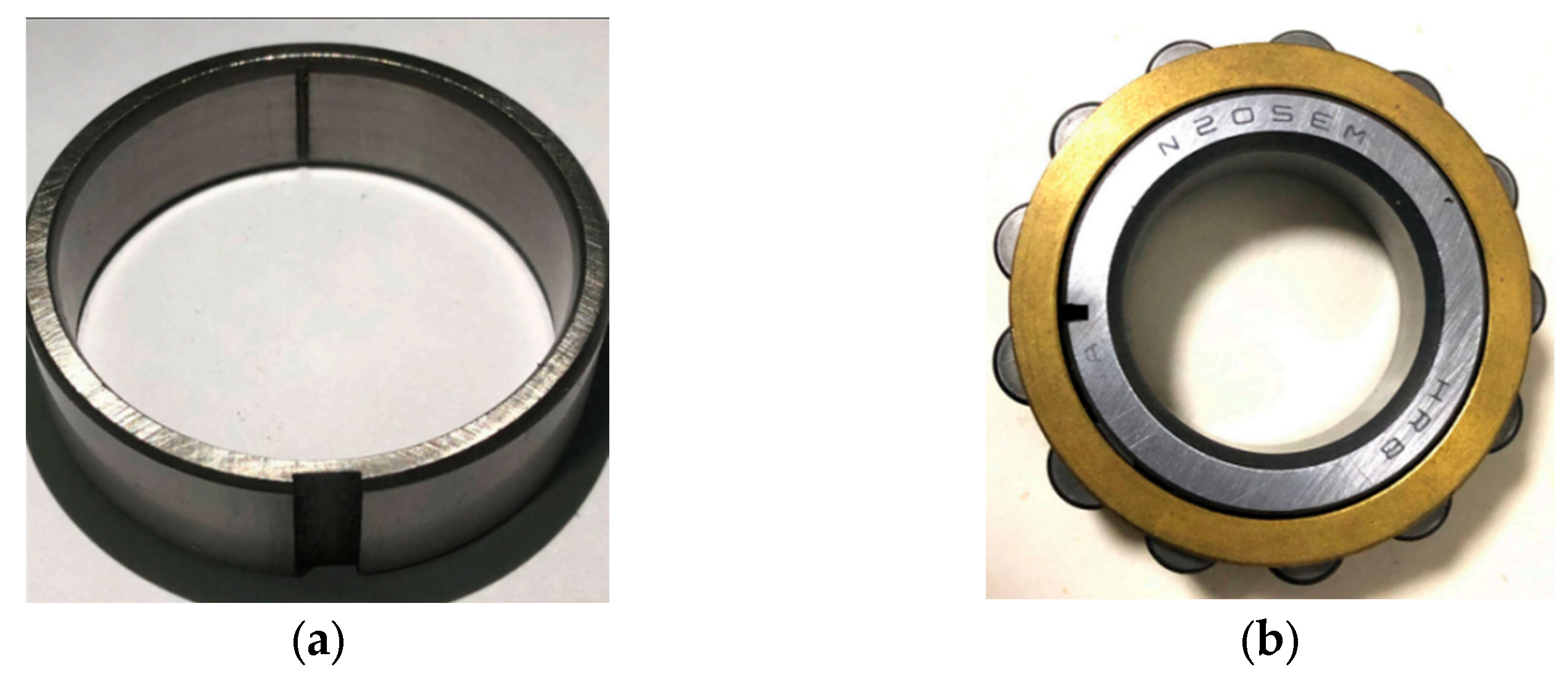
We gathered sound and vibration signals from rolling bearings under different failure forms.

(2)

The acquired signals were subjected to GS-SVR-EEMD noise reduction, respectively, and the effective eigenmode components were outputted.

(3)

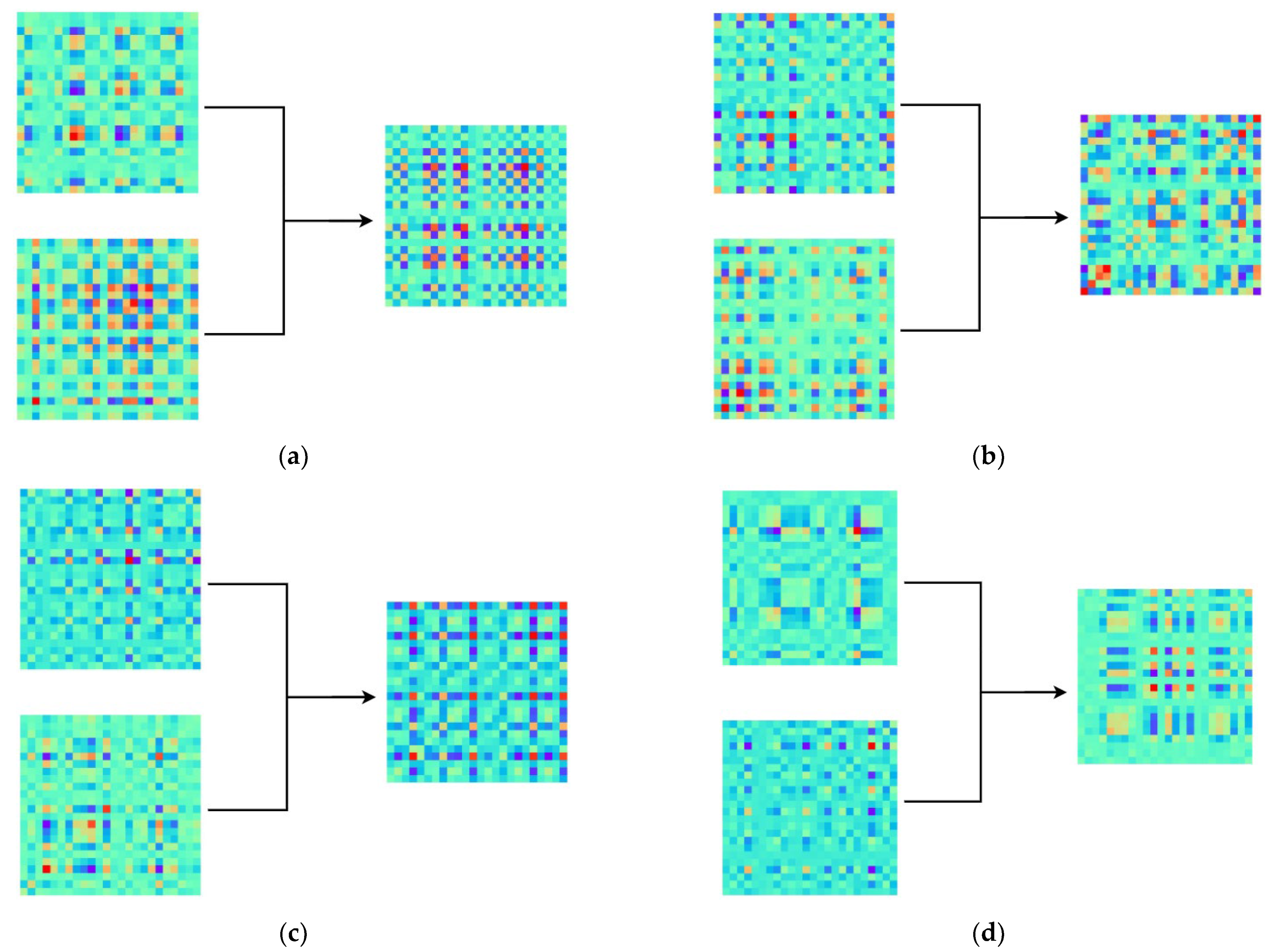
The obtained intrinsic modal components were summed. The processed sound and data signals were obtained. The sound and vibration signals were then subjected to low-rank multimodal fusion.

(4)

The abnormal situations of the sound vibration fusion dataset were checked. Z-score standardization was used to identify abnormal situations. Samples containing anomalies were deleted. The fused signal was converted to a 2D color image by Markov transition fields (MTFs).

(5)

The acquired 2D color images were partitioned into a validation set and a test set in a 3:7 ratio.

(6)

The segmented dataset was subjected to feature classification and recognition using the improved SE-ResNet network.

A flowchart of the experimental method is shown in Figure 7.

Prior to utilizing the enhanced SE-ResNet network, the dataset was transformed into an image-based format in order to facilitate feature extraction. Deep learning models such as ResNet excel in image processing, where key features can be automatically learned. By converting samples into images, the powerful feature extraction capabilities of these models can be better utilized. Moreover, employing images as input data facilitates seamless expansion and modification of the deep learning model’s structure and parameters. This flexibility enables it to adapt to different fault diagnosis tasks.

In the multimodal fusion feature process, the vibration and sound unimodal feature extraction channels $f_v$ and $f_s$ are firstly created using feed-forward neural networks. They are used to extract modal features $Z_v$ and $Z_s$ of the original vibration and sound signal data that have been preprocessed after noise reduction. The obtained modal features are then fused by the LMF method to obtain the final fused features. For specific details, please refer to Reference [25]. The processed vibration and sound signals, respectively, are transformed into 2D images by MTFs.

Figure 8 shows the signal plots of the composite fault (inner ring and outer ring), inner ring fault, outer ring fault, and normal state after acoustic–vibration fusion. It is clear from the 2D image that the signals of the composite fault are more complex than other signals. The 2D image of the composite fault is darker in color. Whether it is the sound signal or the vibration signal, the dark block tends toward the center, which indicates the existence of clustering characteristics of the sound signal and vibration signal. After multimodal fusion, the fault data information is not lost. The sound and vibration signals form a complementary posture. The features of the data are more obvious and it is easier for the convolutional neural network to recognize the fault features.

The images obtained from MTFs were scaled and cropped to pixel 224 × 224 size. In performing model training, the number of training times was set to 100, the data batch size was set to 16, and the learning rate was 0.0001.

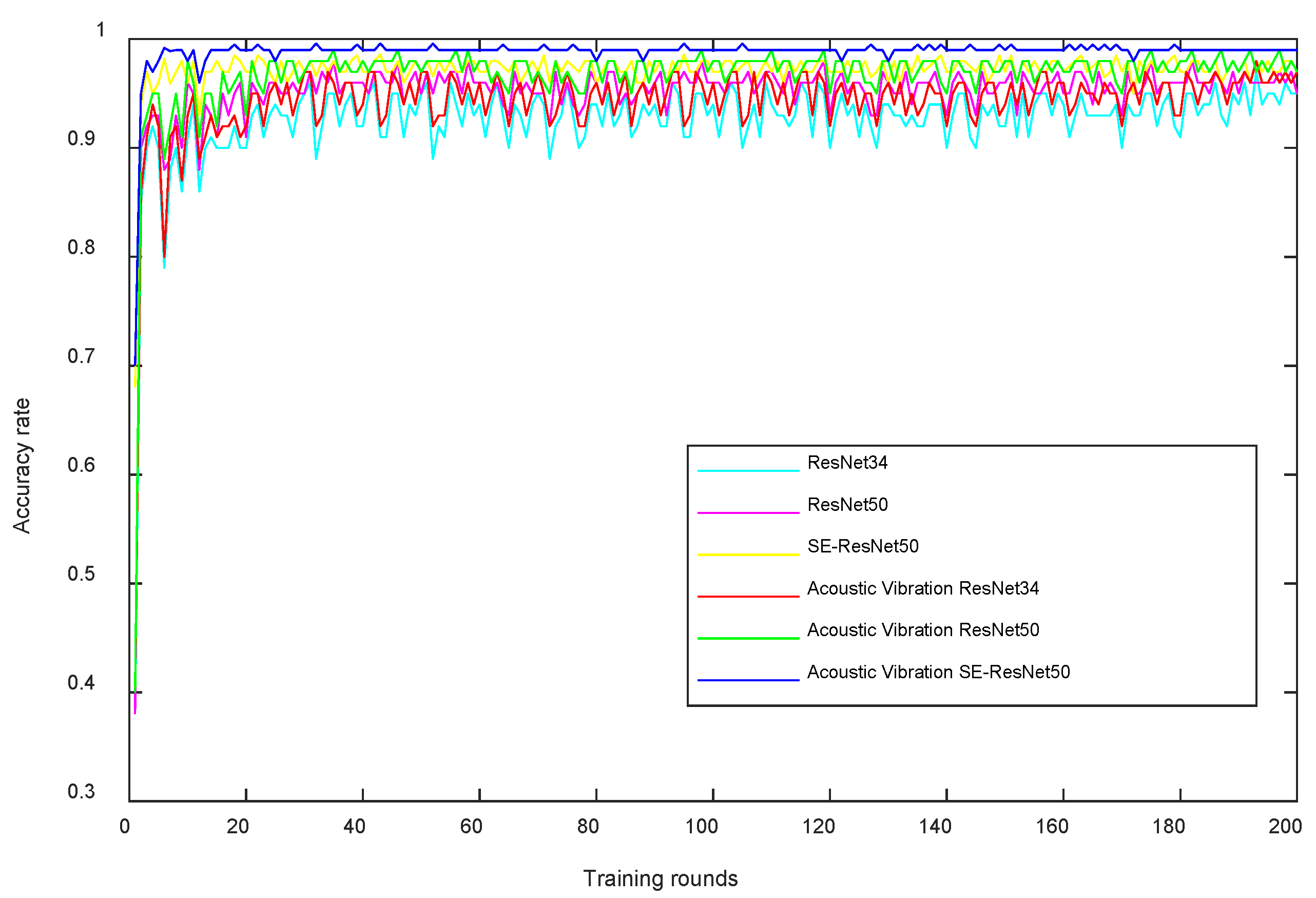
4. Results and Discussion

The ResNet34, ResNet50, SE-ResNet50, VGG-16, and AlexNet networks were used for the classification and identification of features, respectively. The input samples included two forms. One was the sample after the fusion processing of acoustic and vibration data. The sound and vibration signals were fused using the feature fusion method described above. The other was the sample that only contained vibration data. The vibration signal was processed for noise reduction and then the same fault feature classification was conducted.

Table 3. Accuracy of the feature classification.

Input Signal Type	Bearing Status	ResNet34	ResNet50	SE-ResNet50	VGG-16	AlexNet
Feature Classification for Vibration Signal	Normal State	98.03%	98.61%	99.20%	94.22%	92.34%
	Inner Ring Fault	97.41%	98.42%	98.52%	93.82%	91.72%
	Outer Ring Fault	97.52%	98.3%	99.43%	94.03%	91.63%
	Composite Fault	97.86%	98.47%	99.31%	93.16%	91.02%
Runtime/s		12	13	13	25	15
Feature Classification for Acoustic–Vibration Fusion	Normal State	98.64%	98.79%	99.73%	95.12%	92.77%
	Inner Ring Fault	98.66%	99.42%	99.62%	95.76%	92.51%
	Outer Ring Fault	98.31%	98.74%	99.81%	95.54%	91.84%
	Composite Fault	98.29%	99.15%	99.50%	94.79%	91.43%
Runtime/s		11	13	13	25	15

shows the fault feature classification accuracy.

The feature recognition accuracy of SE-ResNet50, based on vibration signals, still outperformed the other networks in fault classification accuracy. For the classification accuracy of outer ring faults, SE-ResNet50 improved by 1.13% over the ResNet50 network. After MTFs were employed, each network model classified fault features more accurately. Under normal conditions, the combined acoustic and vibrational signals improved the accuracy by 0.22% over the vibrational signals. The accuracy increased by 0.7% in the case of inner ring failure. The accuracy increased by 0.17% in the case of outer ring failure. The accuracy increased by 0.47% in the case of the composite fault. This demonstrates that acoustic and vibration signals are complementary in terms of information. By utilizing fused acoustic–vibration input signals, the accuracy of fault diagnosis can be enhanced.

Under identical input conditions, a comparison was made between the execution times of five distinct networks. The findings indicate that the running time of VGG-16 was roughly double that of the other four networks. The running times of ResNet34, ResNet50, SE-ResNet50, and AlexNet were very close to each other. This indicates that the improved SE-ResNet network ensures computational efficiency while improving accuracy.

The MTFs sample set and LMF sample set were individually employed as inputs. Figure 9 and Figure 10 present the performance outcomes of the ResNet34, ResNet50, and SE-ResNet50 models across 200 training sessions. As the number of iterations approaches 10, the loss value steadily converges, indicating the model’s stability and the absence of overfitting. It fully reflects the excellent feature representation ability of MTFs and LMF in signal classification. Different models are compared, highlighting the superiority of sound–vibration fusion. It complements and superimposes the features of sound and vibration signals, making them easier to classify and recognize. Compared to traditional networks, the SE-ResNet50 network demonstrates superior classification capabilities. In the test of acoustic–vibration fusion, SE-ResNet50 converged faster with an accuracy of 99.02%.

5. Conclusions

Targeting the composite fault diagnosis of rolling bearings, an improved SE-ResNet diagnosis method was proposed. Upon experimental verification using bearing data, the following conclusions were reached:

(1)

An improved EEMD method based on GS-SVR with a window function was used for noise reduction of the original signal. The singular value method was used to filter and reconstruct the decomposed IMF components. The pre-processing made the signal easier to analyze.

(2)

The data were converted from Markov variation fields to a 2D image, which facilitated feature recognition by a convolutional neural network. The introduction of SE in the ResNet50 network yielded a great accuracy improvement with a small amount of computation.

(3)

The LMF method was utilized to obtain the sound and vibration signal modal correlation features, and the inter-modal interrelationships were considered. The sophistication of the improved SE-ResNet method for composite fault diagnosis of rolling bearings was demonstrated experimentally.

Furthermore, this article collects data under the same time and rotation speed. The number of samples is controllable. In industrial equipment, the normal operation time is much longer than the fault time. This results in less fault samples. During operation, the noise of mechanical equipment has an immeasurable impact on sound signals. This issue deserves further investigation.

References

1. Jose, E.R.; Jose, A.A.; Claudia, M. Comprehensive diagnosis of localized rolling bearing faults during rotating machine start-up via vibration envelope analysis. Electronics 2024, 13, 375. [Google Scholar]
2. Sumika, C.; Govind, V.; Rajesh, K.; Radoslaw, Z.; Munish, K.G.; Pradeep, K. An adaptive feature mode decomposition based on a novel health indicator for bearing fault diagnosis. Measurement 2024, 226, 114191. [Google Scholar]
3. Gu, H.; Liu, W.; Gao, Q.; Zhang, Y. A review on wind turbines gearbox fault diagnosis methods. J. Vibroeng. 2021, 3, 26–43. [Google Scholar] [CrossRef]
4. Vidal-Puig, S.; Vitale, R.; Ferrer, A. Data-driven supervised fault diagnosis methods based on latent variable models: A comparative study. Chemom. Intell. Lab. Syst. 2019, 187, 41–52. [Google Scholar] [CrossRef]
5. Wang, K.; Gao, B.; Shan, S.; Wang, R.; Wang, X. Research on rolling bearing fault diagnosis method based on ECA-MRANet. Appl. Sci. 2024, 14, 551. [Google Scholar] [CrossRef]
6. Tian, Y.; Pan, G. An unsupervised regularization and dropout based deep neural network and its application for thermal error prediction. Appl. Sci. 2020, 10, 2870. [Google Scholar] [CrossRef]
7. Gu, X.; Xie, Y.; Tian, Y.; Liu, T. A light weight neural network based on GAF and ECA for bearing fault diagnosis. Metals 2023, 13, 822. [Google Scholar] [CrossRef]
8. Mao, W.; He, J.; Li, Y.; Yan, Y. Bearing fault diagnosis with auto-encoder extreme learning machine: A comparative study. Proc. Inst. Mech. Eng. Part C J. Mech. Eng. Sci. 2017, 231, 1560–1578. [Google Scholar] [CrossRef]
9. Saucedo-Dorantes, J.; Arellano-Espitia, F.; Delgado-Prieto, M.; Osornio-Rios, R.A. Diagnosis methodology based on deep feature learning for fault identification in metallic, Hybrid and Ceramic Bearings. Sensors 2021, 21, 5832. [Google Scholar] [CrossRef]
10. Zeng, M.; Li, S.; Li, R.; Lu, J.; Xu, K.; Li, X.; Wang, Y.; Du, J. A hierarchical sparse discriminant autoencoder for bearing fault diagnosis. Appl. Sci. 2022, 12, 818. [Google Scholar] [CrossRef]
11. Liang, P.; Wang, W.; Yuan, X.; Liu, S.; Zhang, L.; Cheng, Y. Intelligent fault diagnosis of rolling bearing based on wavelet transform and improved ResNet under noisy labels and environment. Eng. Appl. Artif. Intell. 2022, 115, 105269. [Google Scholar] [CrossRef]
12. Tao, H.; Wang, P.; Chen, Y.; Stojanovic, V.; Yang, H. An unsupervised fault diagnosis method for rolling bearing using STFT and generative neural networks. J. Frankl. Inst. 2020, 357, 7286–7307. [Google Scholar] [CrossRef]
13. Yang, S.; Yang, P.; Yu, H.; Bai, J.; Feng, W.; Su, Y.; Si, Y. A 2DCNN-RF model for offshore wind turbine high-speed bearing-fault diagnosis under noisy environment. Energies 2022, 15, 3340. [Google Scholar] [CrossRef]
14. Chen, Z.; Gryllias, K.; Li, W. Mechanical fault diagnosis using convolutional neural networks and extreme learning machine. Mech. Syst. Signal Process. 2019, 133, 106272. [Google Scholar] [CrossRef]
15. Pham, M.T.; Kim, J.M.; Kim, C.H. Deep learning-based bearing fault diagnosis method for embedded systems. Sensors 2020, 20, 6886. [Google Scholar] [CrossRef]
16. Zhou, Z.; Wang, H.; Li, Z.; Chen, W. Fault diagnosis of rolling bearing based on deep convolutional neural network and gated recurrent unit. J. Adv. Mech. Des. Syst. Manuf. 2023, 17, JAMDSM0017. [Google Scholar] [CrossRef]
17. Lei, X.; Lu, N.; Chen, C.; Wang, C. An AVMD-DBN-ELM model for bearing fault diagnosis. Sensors 2022, 22, 9369. [Google Scholar] [CrossRef] [PubMed]
18. Jin, T.; Yan, C.; Chen, C.; Yang, Z.; Tian, H.; Wang, S. Light neural network with fewer parameters based on CNN for fault diagnosis of rotating machinery. Measurement 2021, 181, 109639. [Google Scholar] [CrossRef]
19. Khorram, A.; Khalooei, M.; Rezghi, M. End-to-end CNN + LSTM deep learning approach for bearing fault diagnosis. Appl. Intell. 2021, 51, 736–751. [Google Scholar] [CrossRef]
20. Hoang, D.T.; Tran, X.T.; Van, M.; Kang, H.J. A deep Neural Network-Based feature fusion for bearing fault diagnosis. Sensors 2021, 21, 244. [Google Scholar] [CrossRef]
21. Han, H.; Xue, C.; Ma, J.; Cao, X.; Zhang, X. A novel intelligent diagnosis method of rolling bearing and rotor composite faults based on vibration signal-to-image mapping and CNN-SVM. Meas. Sci. Technol. 2023, 34, 044008. [Google Scholar]
22. An, Z.; Wu, F.; Zhang, C.; Ma, J.; Sun, B.; Tang, B.; Liu, Y. Deep learning-based composite fault diagnosis. IEEE J. Emerg. Sel. Top. Circuits Syst. 2023, 13, 572–581. [Google Scholar] [CrossRef]
23. Zhao, Y.; Fan, Y.; Li, H.; Gao, X. Rolling bearing composite fault diagnosis method based on EEMD fusion feature. J. Mech. Sci. Technol. 2022, 36, 4563–4570. [Google Scholar] [CrossRef]
24. Cheng, J.; Yang, Y.; Shao, H.; Pan, H.; Zheng, J.; Cheng, J. Enhanced periodic mode decomposition and its application to composite fault diagnosis of rolling bearings. ISA Trans. 2022, 125, 474–491. [Google Scholar] [CrossRef]
25. Liu, Z.; Shen, Y.; Lakshminarasimhan, V.B.; Liang, P.P.; Bagher Zadeh, A.; Morency, L.P. Efficient low-rank multimodal fusion with modality-specific factors. arXiv 2018, arXiv:180600064. [Google Scholar]
Figure 1. Low-rank multimodal fusion.
Applsci 14 02182 g001
Figure 2. Squeeze and Extraction Module.
Applsci 14 02182 g002
Figure 3. Excitation operation.
Applsci 14 02182 g003
Figure 4. Test rig.
Applsci 14 02182 g004
Figure 5. Sensor arrangement.
Applsci 14 02182 g005
Figure 6. Bearing fault conditions: (a) outer race fault and (b) inner race fault.
Applsci 14 02182 g006
Figure 7. Diagnosis flowchart.
Applsci 14 02182 g007
Figure 8. Diagram of acoustic–vibration fusion: (a) composite fault; (b) inner ring fault; (c) outer ring fault; and (d) normal state.
Applsci 14 02182 g008
Figure 9. Training accuracy.
Applsci 14 02182 g009
Figure 10. Loss comparison.
Applsci 14 02182 g010