Bandgap Dynamics in Locally Resonant Metastructures: A General Theory of Internal Resonator Coupling

Abstract

The dynamics of metastructures, incorporating both conventional and internally coupled resonators, are investigated to enhance vibration suppression capabilities through a novel mathematical framework. A close-form formulation and a transfer function methodology are introduced, integrating control system theory with metastructure analysis, offering new insights into the role of internal coupling. The findings reveal that precise internal coupling, when matched exactly to the stiffness of the resonator, enables the clear formation of secondary bandgaps, significantly influencing the vibration isolation efficacy of the metastructure. Although the study primarily focuses on theoretical and numerical analyses, the implications of adjusting mass distribution on resonators are also explored. This formulation methodology enables the adjustment of bandgap characteristics, underscoring the potential for adaptive control over bandgaps in metastructures. Such capabilities are crucial for tailoring the vibration isolation and energy harvesting functionalities in mechanically resonant systems, especially when applied to demanding heavy-duty applications.

1. Introduction

Locally resonant metamaterials have revolutionized the field of material science by enabling the manipulation of mechanical waves through unique structural designs that are not possible with conventional materials. Such metamaterials utilize an intricate arrangement of embedded resonators to selectively amplify or attenuate waves, yielding capabilities like enhanced vibration isolation, targeted wave trapping, and precise steering. The cross-disciplinary value of these materials is evident in their wide-ranging applications, from improving acoustic insulation and energy harvesting to managing seismic waves and developing advanced sensors.

The concept of metamaterials is not exclusive to structural dynamics; its origins can be traced back to research in optics by Shelby et al. [1], and it has since become a subject of extensive study in various fields, including acoustics. Moreover, the concept of mechanical locally resonant metamaterials was first introduced by Liu et al. [2], who demonstrated an elastic locally resonant bandgap phenomenon, akin to a mass-spring oscillator. Since then, various types of mechanical locally resonant metamaterials have been extensively investigated in the literature.

The field of resonator couplings and dispersion has seen substantial progress in recent years. For instance, Hazra et al. [3] innovated a superconducting architecture utilizing a ring resonator for multiqubit connectivity, enhancing the efficiency of quantum processors. In the realm of optics and spectroscopy, Rozenman et al. [4] developed a novel experimental setup to measure the dispersion of organic exciton polaritons, revealing the quantized interactions between light and matter in organic materials. Additionally, Li et al. [5] demonstrated the coherent internally coupled distant magnonic resonators via superconducting circuits for integrated magnonic networks that can operate coherently at quantum-compatible scales.

From optics and materials science to structural vibration and energy harvesting, these advancements bridge diverse fields to pioneer new applications and efficiencies. Hu et al. [6] proposed a modified metamaterial beam that combined vibration suppression and energy harvesting functions in internally coupled resonators in the low-frequency range. In their design, local resonators were alternately coupled, with piezoelectric elements attached for energy conversion. Oyelade and Oladimeji [7] also contributed by introducing a novel metamaterial with a multiresonator mass-in-mass lattice system, where the internal coupling was achieved through a linear spring, leading to the formation of two additional bandgaps over conventional designs.

The research trajectory in metastructure system formulation has been significantly advanced by Erturk et al. [8], who developed a robust framework that culminates in transfer functions, allowing for nuanced manipulation and control of system responses. Sugino et al.’s mathematical framework, leveraging Laplace transformations, further simplifies the analysis of metastructures, especially in damping low-frequency vibrations, thus enhancing the practical applicability of these complex systems in engineering solutions. Sugino et al. [9] developed the mathematical framework using Laplace transformations for analyzing locally resonant metastructures, simplifying examination of their responses, and deriving a closed-form expression for bandgap frequency range, validated through dispersion analysis and experimental tests.

Traditional methods focus on dispersion analysis and limit the scope of analysis to wave propagation without offering insights into control strategies. This work develops a mathematical framework to derive a close-form formulation for analyzing both conventional and internally coupled resonators in metastructures, integrating control system theory and the transfer function method to provide enhanced control mechanisms and bandgap tuning methods through resonator stiffness adjustments. This advancement has the potential to revolutionize metastructural design for industrial applications, enabling the creation of structures with multiple bandgaps and diverse functionalities.

This framework not only enhances our understanding of metastructures but also provides novel methods for tuning bandgaps, thereby improving vibration isolation and facilitating energy harvesting. With implications spanning industrial machinery and noise cancellation, these advancements promise to revolutionize engineering practices by enabling more efficient and effective control mechanisms in various industrial applications.

This work addresses the knowledge gap in linear internal coupling in metastructures, and aims to improve wave manipulation and dynamic control through a new mathematical framework, expanding the applications and functionalities of metastructures.

It claims that transfer function methodology can model and control metastructure dynamics, including internally coupled resonators. It highlights a gap in understanding linear internal coupling effects on bandgap manipulation, and demonstrates the maintenance of primary bandgaps and the emergence of secondary bandgaps through internal coupling, suggesting adjustable resonator mass distribution for further tuning.

This leads to the following research questions:

• How does internal coupling affect the bandgap characteristics of a metastructure?
• What is the role of internal coupling in enhancing or merging bandgaps for vibration isolation in continuous (distributed) metastructures?
• Can the integration of control system theory and transfer function methodology lead to real-time adaptive tuning of metastructure bandgaps?
• Can an alternative method, such as modifying the mass distribution on resonators, offer a practical way to alter bandgap characteristics without restructuring, while also being suitable for heavy-duty applications where piezoelectric solutions are less viable?

The key contributions of this paper are as follows:

• We enable the transfer function approach as an analysis method for metastructures, enhancing dynamic bandgap characteristics through the use of different functionalities and precise control engineering techniques.
• We develop a mathematical method for formulating closed-form equations describing the behaviors of internally coupled resonators, providing a deeper understanding of their impact on metastructure dynamics.
• We address the challenge of merging bandgaps from internally coupled and conventional resonators, offering insights into continuous vibration control in distributed systems.

The structure of the remaining sections of this paper is as follows: Section 2 delves into the methodology, detailing the theoretical foundations and optimization strategies employed for bandgap generation. Results and discussion are presented in Section 3, where the implications of the applied methodologies are interpreted in the context of mechanical system design and enhancement. A “Finite Element Study” is detailed in Section 4, showcasing the vibrational behaviors and bandgap characteristics of the metastructures under study. This section includes a focused examination of the effects of spatial variations on bandgap properties, emphasizing the utility and implications of these findings for practical applications. Finally, Section 5 concludes the paper, summarizing the key findings and proposing directions for future research.

2. Modal Analysis and Bandgap Formation in Mechanical Metastructures

The research primarily employs modal analysis in the design and optimization of mechanical locally resonant metastructures. This analysis is crucial for identifying key vibration characteristics, such as natural frequencies, mode shapes, and modal damping ratios, under specific conditions. These insights enable the engineering of metastructures with tailored mechanical wave propagation behaviors.

The study employs a distributed parameter model approach, utilizing partial differential equations (PDEs) to capture the system dynamics more precisely than lumped parameter models. This methodology is particularly applicable to systems where spatial variations are non-negligible, affecting phenomena such as wave propagation, heat transfer, and fluid dynamics. Analytical models are derived using modal analysis through the frequency determinant method, providing a solid theoretical foundation for understanding the intricate behavior of internally coupled resonators within metastructures.

The standard distributed model of the metastructure under investigation, subject to base excitation and external forces, is illustrated in Figure 1. Employing Newtonian mechanics and drawing from classical vibration textbooks, the behavior of the metastructure is captured by the following partial differential equation, as detailed in Equation (1).

$$\mathcal{L}w(x,t)+\mathcal{C}\frac{\partial w(x,t)}{\partial t}+\mathcal{M}\frac{{\partial }^{2}w(x,t)}{\partial t^2}-\sum _{r=1}^{N_r}\left(k_r{z}_r\left(t\right)+c_r\frac{\partial z_r\left(t\right)}{\partial t}\right)\delta \left(x-x_r\right)={\mathcal{F}}_{b_m}(x,t)$$

(1)

which includes structural flexibility $\mathcal{L}$, damping $\mathcal{C}$, and inertia $\mathcal{M}$. The interaction with the resonators is represented by the summation term, encompassing the stiffness $k_r$, damping $c_r$, and location $x_r$ of each resonator. The dynamic of the system is a linear homogeneous differential operator, exhibiting orders of $2p$ and $2q$, respectively, with $q\le p$. The spatial coordinate x extends over domain D. The function $w(x,t)$ captures the system’s relative transverse vibration compared to the base motion, essentially reflecting the displacement at specific points relative to the base’s harmonic movement. On the other hand, $z_r\left(t\right)$ denotes the resonator’s relative vibration in absolute coordinates, providing insight into its displacement to the overall structure’s vibration. The $\delta (x-x_r)$ is the Kronecker delta function to pinpoint the resonators’ locations on the beam, with $x_r$ specifying the position of the r-th resonator. Moreover, $\mathcal{F}$ symbolizes the external force, distributed across D, and incorporates the impact of the base excitation on the beam.

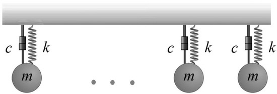
Figure 1. Example of standard locally resonant metastructures, where m represents the mass of the resonators, c is the damping, and k is the stiffness of the resonators.

Similarly, the governing equation for the resonators, derived from Newton’s second law of motion, is expressed as follows:

$$m_r\frac{{\partial }^2{z}_r\left(t\right)}{\partial t^2}+c_r\frac{\partial z_r\left(t\right)}{\partial t}+k_r{z}_r\left(t\right)+m_r\frac{{\partial }^{2}w\left(x_r,t\right)}{\partial t^2}={\mathcal{F}}_{b_r}\left(t\right)$$

(2)

The boundary conditions for the system, as outlined in Equation (1), are defined by Equation (3), where each ${\mathcal{B}}_i$ is a linear homogeneous differential operator of order no greater than $2p-1$.

$${\mathcal{B}}_i\left[w(x,t)\right]=0,i=1,2,\dots ,p$$

(3)

Proportional damping, a method often used in real-world structures for estimating natural frequencies and mode shapes, relates the damping matrix to the mass and stiffness matrices. This concept allows $\mathcal{C}$ to be expressed as a combination of mass and stiffness operators $\mathcal{L}$ and $\mathcal{M}$, as shown in Equation (4), with $c_1$ and $c_2$ being non-negative constants, determined based on the physical properties of the system. However, engineers usually use experimental modal analysis or fit data from vibration tests to find them. This approach, as referenced in [10], maintains consistent mode shapes and similar natural frequencies for both damped and undamped systems.

$$\mathcal{C}=c_1\mathcal{L}+c_2\mathcal{M}$$

(4)

The eigenfunctions ${\varphi }_m\left(x\right)$ of the system are derived by solving the eigenvalue problem of the undamped version of Equation (1), presented in Equation (5).

$$\mathcal{L}\left[{\varphi }_m\left(x\right)\right]={\lambda }_m\mathcal{M}\left[{\varphi }_m\left(x\right)\right],m=1,2,\dots ,N_m$$

(5)

The symbol ${\lambda }_m$ represents an eigenvalue associated with the mth eigenfunction ${\varphi }_m\left(x\right)$ of the system. For structures like beams equipped with resonators, the system is defined by coupled differential equations for each resonator and the structure itself. These equations account for the mutual influence of each component on the system’s dynamics. The mode shapes of the base structure alone are not the exact mode shapes of the entire metastructure, but using them simplifies the analysis significantly. The solution to Equation (5) is provided in Appendix A.

In the case of an Euler beam spanning domain $D=[0,L]$, assumed to be linearly elastic and homogeneous, the operators $\mathcal{L}$, $\mathcal{M}$, $\mathcal{C}$, ${\mathcal{B}}_1$, and ${\mathcal{B}}_2$ are defined in terms of the beam’s physical properties: flexural rigidity ($EI$), density ($\rho$), and cross-sectional area (A).

$$\begin{array}{cc}\hfill \mathcal{L}& =EI\frac{{\partial }^4}{\partial x^4},\mathcal{M}=\rho A,\mathcal{C}=c,\hfill \\ \hfill {\mathcal{B}}_1& =1,{\mathcal{B}}_2=EI\frac{{\partial }^2}{\partial x^2}\hfill \end{array}$$

(6)

In advancing the understanding of modal expansion in the system, the orthogonality of eigenfunctions is critical for solving Equation (1). The self-adjoint (Hermitian) nature of the eigenvalue problem ensures this orthogonality. For any two eigenfunctions ${\varphi }_m\left(x\right)$ and ${\varphi }_n\left(x\right)$, the problem is self-adjoint if they satisfy the conditions given in Equation (7), as highlighted by [11].

$$\begin{array}{c}{\int }_D{\varphi }_m\left(x\right)\mathcal{L}\left[{\varphi }_n\left(x\right)\right]dx={\int }_D{\varphi }_n\left(x\right)\mathcal{L}\left[{\varphi }_m\left(x\right)\right]dx\\ {\int }_D{\varphi }_m\left(x\right)\mathcal{M}\left[{\varphi }_n\left(x\right)\right]dx={\int }_D{\varphi }_n\left(x\right)\mathcal{M}\left[{\varphi }_m\left(x\right)\right]dx.\end{array}$$

(7)

When considering unique eigenvalues ${\omega }_m^2$ and ${\omega }_n^2$ with their respective eigenfunctions ${\varphi }_m\left(x\right)$ and ${\varphi }_n\left(x\right)$, these functions are normalized with respect to $\mathcal{M}$. This normalization leads to the generalized orthogonality condition outlined in Equations (8) and (9), with ${\delta }_{mn}$ being the Kronecker delta function.

$${\int }_D{\varphi }_m\left(x\right)\mathcal{M}\left[{\varphi }_n\left(x\right)\right]dx={\delta }_{mn}$$

(8)

and

$${\int }_D{\varphi }_m\left(x\right)\mathcal{L}\left[{\varphi }_n\left(x\right)\right]dx={\delta }_{mn}{\omega }_m^2$$

(9)

Assuming proportional damping, the structural damping characteristics are captured by Equation (10). Here, ${\zeta }_m$ denotes the damping ratio of the m-th mode, which is precisely defined in Equation (11) utilizing the constants $c_1$ and $c_2$. Equations (8)–(10) are integral to constructing a set of orthonormal eigenfunctions, which together form a complete basis for the solution space pertinent to the eigenvalue problem.

$${\int }_D{\varphi }_m\left(x\right)\mathcal{C}\left[w_m\left(x\right)\right]dx=c_1{\delta }_{mn}{\omega }_m^2+c_2{\delta }_{mn}=2{\delta }_{mn}{\zeta }_m{\omega }_m$$

(10)

with

$${\zeta }_m=\frac{1}{2{\omega }_m}\left(c_1{\omega }_m^2+c_2\right)$$

(11)

Modal decomposition is a method used to describe the structure’s vibration across a domain D by representing it as a sum of modal shapes in one direction. This method assumes that the behavior of the structure can be accurately captured using a finite set of modes. For instance, the Euler–Bernoulli beam theory, commonly used in these analyses, may not provide sufficient accuracy in high-frequency situations. This technique, widely used in modal analysis, produces convergent solutions to the boundary value problem as formulated.

Using modal decomposition, the beam’s deflection in the domain D is expressed as a sum of modal shapes in one direction. This assumes that the behavior of the beam can be accurately represented by a finite number of modes, as expressed in Equation (12):

$$w(x,t)=\sum _{m=1}^{N_m}{\varphi }_m\left(x\right)z_m\left(t\right),$$

(12)

Here, ${\varphi }_m\left(x\right)$ denotes the spatial mode shape, and $z_m\left(t\right)$ is the time-dependent modal coordinate for the m-th mode. These modal representations are crucial in modeling the dynamics of a flexible beam with integrated discrete resonators.

Incorporating the modal expansion from Equation (12) into the system’s governing differential equation, given by Equation (1), yields Equation (13). This resultant equation effectively combines the modal decomposition with the system’s differential operators, capturing the influence of the resonators. It provides a complete representation of the beam’s dynamic response, encompassing both the modal characteristics and the interactive effects of the resonators.

$$\begin{array}{cc}\hfill & \mathcal{L}\sum _{m=1}^{N_m}{\varphi }_m\left(x\right)z_m\left(t\right)+\mathcal{C}\frac{\partial }{\partial t}\sum _{m=1}^{N_m}{\varphi }_m\left(x\right)z_m\left(t\right)+\mathcal{M}\frac{{\partial }^2}{\partial t^2}\sum _{m=1}^{N_m}{\varphi }_m\left(x\right)z_m\left(t\right)-\hfill \\ \hfill & \sum _{r=1}^{N_r}\left(k_r{z}_r\left(t\right)+c_r\frac{d{z}_r\left(t\right)}{dt}\right)\delta \left(x-x_r\right)={\mathcal{F}}_{b_m}(x,t)\hfill \end{array}$$

(13)

Multiplying Equation (13) by ${\varphi }_n\left(x\right)$ and integrating over the domain D, and applying the orthogonality conditions Equations (8)–(11) of the mode shapes, gives

$${\ddot{z}}_m\left(t\right)+2{\zeta }_m{\omega }_m{\dot{z}}_m\left(t\right)+{\omega }_m^2{z}_m\left(t\right)-\sum _{r=1}^{N_r}{m}_r{\omega }_r^2{z}_r\left(t\right){\varphi }_m\left(x_r\right)={\mathcal{Q}}_{b_m}(x,t),m=1,2,\dots ,N_m$$

(14)

Similarly for resonators, substituting the modal expansion Equations (12) into (2) yields

$${\ddot{z}}_r\left(t\right)+2{\zeta }_r{\omega }_r{\dot{z}}_r\left(t\right)+{\omega }_r^2{z}_r\left(t\right)+\sum _{m=1}^{N_m}{\ddot{z}}_m\left(t\right){\varphi }_m\left(x_r\right)={\mathcal{Q}}_{b_r}\left(t\right),r=1,2,\dots ,N_r$$

(15)

Here, $N_m$ and $N_r$ denote the number of modes and resonators, respectively. Each mode has a specific modal frequency ${\omega }_m$, and each resonator has a mass $m_r$ and its own natural frequency ${\omega }_r$. The damping ratios ${\zeta }_m$ for the modes and ${\zeta }_r$ for the resonators quantify energy dissipation.

To simplify, the superscript “dot” indicates time derivatives, and “prime” indicates spatial derivatives. Each equation in the model represents the dynamics of modal coordinates or resonator displacement as a second-order ordinary differential equation. The dynamics are influenced by modal and resonator parameters (natural frequencies ${\omega }_m$ and ${\omega }_r$, damping ratios ${\zeta }_m$ and ${\zeta }_r$), their interactions, and base excitation forces (${\mathcal{Q}}_{b_m}$ and ${\mathcal{Q}}_{b_r}$).

Decoupling of these equations is achieved through an orthogonal transformation, involving pre- and post-multiplication by the mode shape matrix. This leads to diagonalization of the mass and stiffness matrices, thanks to the orthogonality of eigenvectors to both matrices. The result is a set of decoupled ordinary differential equations. This normal mode method applies in the absence of damping or with proportional damping, where the damping matrix is a linear combination of the mass and stiffness matrices. The transformation becomes orthonormal when the mode shape is normalized to the mass matrix.

Combining the structural dynamics represented in Equation (14) with the dynamics of resonators from Equation (15) enables the coupling of inertial terms and decoupling of stiffness in the system, facilitating analysis in the frequency domain. This process is expressed in Equation (16), where ${\mathcal{H}}_{b_m}(x,t)$ is determined by integrating the effects of external forces, base motion, and damping into a net external force, as shown in Equation (17). Equations (15) and (16) together form a set of coupled second-order linear ordinary differential equations, which, upon solving, yield the mode shapes and resonant frequencies of the entire system and its steady-state response to harmonic excitation.

$$\begin{array}{cc}\hfill & {\ddot{z}}_m\left(t\right)+2{\zeta }_m{\omega }_m{\dot{z}}_m\left(t\right)+{\omega }_m^2{z}_m\left(t\right)+\sum _{r=1}^{N_r}{m}_r{\varphi }_m\left(x_r\right)\sum _{p=1}^{N_m}{\ddot{z}}_m\left(t\right){\varphi }_p\left(x_r\right)+\hfill \\ \hfill & \sum _{r=1}^{N_r}{m}_r{\ddot{z}}_r\left(t\right){\varphi }_m\left(x_r\right)+2\sum _{r=1}^{N_r}{m}_r{\varphi }_m\left(x_r\right){\zeta }_r{\omega }_r{\dot{z}}_r\left(t\right)={\mathcal{H}}_{b_m}(x,t),m=1,2,\dots ,N_m\hfill \end{array}$$

(16)

$$\begin{array}{cc}\hfill & {\mathcal{H}}_{b_m}(x,t)={\int }_0^L{\mathcal{F}}_e(x,t){\varphi }_m\left(x\right)dx-{\ddot{w}}_b\left(t\right)\left({\int }_0^L\mathcal{M}{\varphi }_m\left(x\right)dx+\sum _{r=1}^{N_r}{m}_r{\varphi }_m\left(x_r\right)\right)-\hfill \\ \hfill & {\dot{w}}_b\left(t\right){\int }_0^L\mathcal{C}{\varphi }_m\left(x\right)dx\hfill \end{array}$$

(17)

The Laplace transform is applied to the system of equations, assuming zero initial conditions, to transition the analysis to the frequency domain, as seen in Equations (18) and (19). In these equations, $Z_m\left(s\right)$ and $Z_r\left(s\right)$ represent the Laplace transforms of the modal and resonator displacements, respectively. This transformation simplifies the algebraic manipulation and analysis of the system’s dynamics.

$$Z_r\left(s\right)=\frac{{\mathcal{Q}}_{b_r}\left(s\right)-{\sum }_{m=1}^{N_m}{s}^2{Z}_m\left(s\right){\varphi }_m\left(x_r\right)}{s^2+2{\zeta }_r{\omega }_{r}s+{\omega }_r^2},r=1,2,\dots ,N_r$$

(18)

$$\begin{array}{cc}\hfill & s^2{Z}_m\left(s\right)+2{\zeta }_m{\omega }_{m}s{Z}_m\left(s\right)+{\omega }_m^2{Z}_m\left(s\right)+\sum _{r=1}^{N_r}{m}_r{\varphi }_m\left(x_r\right)\sum _{p=1}^{N_m}{s}^2{Z}_p\left(s\right){\varphi }_p\left(x_r\right)+\hfill \\ \hfill & \sum _{r=1}^{N_r}{m}_r{s}^2{Z}_r\left(s\right){\varphi }_m\left(x_r\right)+2\sum _{r=1}^{N_r}{m}_r{\varphi }_m\left(x_r\right){\zeta }_r{\omega }_{r}s{Z}_r\left(s\right)=H_{b_m}\left(s\right),m=1,2,\dots ,N_m\hfill \end{array}$$

(19)

For a deeper analytical understanding, applying Equation (18) to the Laplace transform of Equation (14) yields the following expression in Equation (20).

$$\begin{array}{cc}\hfill & (s^2+2{\zeta }_m{\omega }_{m}s+{\omega }_m^2)Z_m\left(s\right)-\sum _{r=1}^{N_r}{m}_r{\omega }_r^2\left(\frac{{\mathcal{Q}}_{b_r}\left(s\right)-{\sum }_{p=1}^{N_m}{s}^2{Z}_p\left(s\right){\varphi }_p\left(x_r\right)}{s^2+2{\zeta }_r{\omega }_{r}s+{\omega }_r^2}\right){\varphi }_m\left(x_r\right)={\mathcal{Q}}_{b_m}\left(s\right),\hfill \\ \hfill & m=1,2,\dots ,N_m\hfill \end{array}$$

(20)

The analysis focuses on the transfer function $\frac{Z_m}{{\mathcal{Q}}_{b_m}}$, particularly when the effect of ${\mathcal{Q}}_{b_r}$ is ignored. Here, the mass ratio $\mu$, a dimensionless quantity, relates the mass of each resonator to a differential mass element of the system and is defined as $\mu =\frac{m_r}{m\left(x_r\right)d{x}_r}$, where $m\left(x_r\right)$ represents the mass per unit length at $x_r$ and $d{x}_r$ is an infinitesimal segment length at this point. To simplify the system of equations, it is assumed that an infinite number of resonators are distributed throughout the entire domain of x, and the regions represented by $x_r$ become infinitesimally small.

$$\underset{N_r\to \infty }{lim}\sum _{r=1}^{N_r}m\left(x_r\right){\varphi }_m\left(x_r\right){\varphi }_p\left(x_r\right)d{x}_r\approx {\int }_0^{L}m\left(x\right){\varphi }_m\left(x\right){\varphi }_p\left(x\right)dx={\delta }_{mp},m,p=1,2,\dots$$

(21)

Applying these assumptions results in the following expression:

$$\begin{array}{cc}\hfill & \frac{Z_m\left(s\right)}{Q_{b_m}\left(s\right)}=\frac{1}{s^2\left(1+\frac{\mu (2{\zeta }_r{\omega }_{r}s+{\omega }_r^2)}{s^2+2{\zeta }_r{\omega }_{r}s+{\omega }_r^2}\right)+2{\zeta }_m{\omega }_{m}s+{\omega }_m^2}\hfill \\ \hfill & m=1,2,\dots ,N_m\hfill \end{array}$$

(22)

Equation (22) indicates that resonators add a frequency-dependent mass to the system. With the assumption of an infinite resonator distribution, leading to continuous spatial displacements, similar reductions apply to the resonator displacements. By substituting Equations (22) into (18) and transitioning from the discrete $x_r$ to a continuous spatial domain x, a simplified equation emerges as presented in Equation (23).

$$Z_r(x,s)=-\frac{s^2}{s^2+2{\zeta }_r{\omega }_{r}s+{\omega }_r^2}\sum _{m=1}^{N_m}\frac{Q_{b_m}\left(s\right){\varphi }_m\left(x\right)}{s^2\left(1+\frac{\mu ({\omega }_r^2+2{\zeta }_r{\omega }_{r}s)}{s^2+2{\zeta }_r{\omega }_{r}s+{\omega }_r^2}\right)+2{\zeta }_m{\omega }_{m}s+{\omega }_m^2}$$

(23)

Equation (23) defines the motion $Z_r(x,s)$ of resonators along the beam in the Laplace domain, influenced by modal forces $Q_{b_m}\left(s\right)$. The displacement of the resonators is presented as a weighted sum of the beam’s modal shapes:

$$Z_r(x,s)=\sum _{m=1}^{N_m}{\Psi }_m\left(s\right){\varphi }_m\left(x\right)$$

(24)

Equation (25) expresses the relationship between the modal force $Q_{b_m}\left(s\right)$ and the modal coordinate ${\Psi }_m\left(s\right)$ in the Laplace domain. It illustrates how resonator displacements are influenced by the modes of the structure:

$$\frac{{\Psi }_m\left(s\right)}{Q_{b_m}\left(s\right)}=\frac{-s^2}{\left[s^2+2{\zeta }_r{\omega }_{r}s+{\omega }_r^2\right]\left[s^2\left(1+\frac{\mu ({\omega }_r^2+2{\zeta }_r{\omega }_{r}s)}{s^2+2{\zeta }_r{\omega }_{r}s+{\omega }_r^2}\right)+2{\zeta }_m{\omega }_{m}s+{\omega }_m^2\right]},m=1,2,\dots ,N_m$$

(25)

The transfer function in Equation (25) clarifies how the input forces are transformed into modal responses. The function’s poles, indicative of the system’s natural frequencies, are the points at which the system exhibits peak responses.

By introducing an internal linear coupling term, $\kappa$, within the resonators illustrated in Figure 2, the system evolves into internally coupled resonators. This transformation creates an environment where the displacements of the resonators are no longer independent but are coupled. Specifically, the displacement of one resonator influences the displacement of the other, establishing a dynamic interaction. The energy associated with this coupling is quantified by the coupling potential energy, in which each pair of resonators (1 and 2, 3 and 4, 5 and 6, etc.) forms a system with two degrees of freedom: $V_c\left(t\right)=\frac{1}{2}\kappa {\left(z_{r_1}\left(t\right)-z_{r_2}\left(t\right)+w\left(x_{r_1},t\right)-w\left(x_{r_2},t\right)\right)}^2$. The equations for the coupled oscillator system can be formulated as follows:

$$\begin{array}{cc}\hfill & {\ddot{z}}_m\left(t\right)+2{\zeta }_m{\omega }_m{\dot{z}}_m\left(t\right)+{\omega }_m^2{z}_m\left(t\right)-\sum _{r=1}^{N_r/2}\left(m_{2r-1}{\omega }_{2r-1}^2{z}_{2r-1}\left(t\right){\varphi }_m\left(x_{2r-1}\right)\right.+\hfill \\ \hfill & \left.m_{2r}{\omega }_{2r}^2{z}_{2r}\left(t\right){\varphi }_m\left(x_{2r}\right)\right)={\mathcal{Q}}_{b_m},m=1,2,\dots ,N_m,\mathrm{and}{N}_r\in 2\mathbb{N}\hfill \end{array}$$

(26)

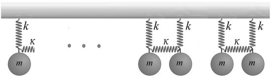
Figure 2. Locally resonant metastructures with internally coupled resonators. Each pair of resonators forms one unit cell, with m representing the mass of the resonators, c the damping, k the stiffness of the resonators, and $\kappa$ the internal coupling stiffness between them.

Meanwhile, the equation for the resonators is given by the following:

$$\begin{array}{cc}\hfill & {\ddot{z}}_{2r-1}\left(t\right)+2{\xi }_{2r-1}{\omega }_{2r-1}{\dot{z}}_{2r-1}\left(t\right)+{\omega }_{2r-1}^2{z}_{2r-1}\left(t\right)+\sum _{m=1}^{N_m}{\ddot{z}}_m\left(t\right){\varphi }_m\left(x_{2r-1}\right)+\hfill \\ \hfill & \beta \frac{\kappa }{m_{2r-1}}={\mathcal{Q}}_{b_{2r-1}},r=1,2,\dots ,N_r/2\hfill \end{array}$$

(27)

$$\begin{array}{cc}\hfill & {\ddot{z}}_{2r}\left(t\right)+2{\xi }_{2r}{\omega }_{2r}{\dot{z}}_{2r}\left(t\right)+{\omega }_{2r}^2{z}_{2r}\left(t\right)+\sum _{m=1}^{N_m}{\ddot{z}}_m\left(t\right){\varphi }_m\left(x_{2r}\right)\hfill \\ \hfill & -\beta \frac{\kappa }{m_{2r}}={\mathcal{Q}}_{b_{2r}},r=1,2,\dots ,N_r/2\hfill \end{array}$$

(28)

where

$$\beta =z_{2r-1}\left(t\right)-z_{2r}\left(t\right)+\sum _{m=1}^{N_m}{z}_m\left(t\right){\varphi }_m\left(x_{2r-1}\right)-\sum _{m=1}^{N_m}{z}_m\left(t\right){\varphi }_m\left(x_{2r}\right)$$

(29)

These equations characterize the underlying dynamics of both the beam and the internally linear coupled resonator system. The Laplace transform of Equation (26) with zero initial conditions results in Equation (30).

$$\begin{array}{cc}\hfill & (s^2+2{\zeta }_m{\omega }_{m}s+{\omega }_m^2)Z_m\left(s\right)-\sum _{r=1}^{N_r/2}\left(m_{2r-1}{\omega }_{2r-1}^2{Z}_{2r-1}\left(s\right){\varphi }_m\left(x_{2r-1}\right)+\right.\hfill \\ \hfill & \left.m_{2r}{\omega }_{2r}^2{Z}_{2r}\left(s\right){\varphi }_m\left(x_{2r}\right)\right)=Q_{b_m}\left(s\right)\hfill \end{array}$$

(30)

Given that the forces ${\mathcal{Q}}_{b_{2r-1}}$ and ${\mathcal{Q}}_{b_{2r}}$ are equal to $-{\ddot{w}}_b\left(t\right)$, and considering that $m_{2r-1}=m_{2r}$ or identical mass $m_r$ for all resonators, along with the distribution of numerous resonators along a beam, it is assumed that the derivative of position within each unit cell is the same, indicated by $d{x}_{2r-1}=d{x}_{2r}$. This reflects a uniform position derivative across all resonators. Furthermore, the following relationships are established: $m_{2r-1}=\mu m\left(x_{2r-1}\right)d{x}_{2r-1}$, and $m_{2r}=\mu m\left(x_{2r}\right)d{x}_{2r}$.

$$\underset{N_r\to \infty }{lim}\sum _{r=1}^{N_r/2}m\left(x_{2r-1}\right){\varphi }_m\left(x_{2r-1}\right){\varphi }_p\left(x_{2r-1}\right)d{x}_{2r-1}=\frac{1}{2}{\delta }_{mp},m,p=1,2,\dots$$

(31)

$$\underset{N_r\to \infty }{lim}\sum _{r=1}^{N_r/2}m\left(x_{2r}\right){\varphi }_m\left(x_{2r}\right){\varphi }_p\left(x_{2r}\right)d{x}_{2r}=\frac{1}{2}{\delta }_{mp},m,p=1,2,\dots$$

(32)

Taking the Laplace transform of Equations (27) and (28), and applying the orthogonality of the mode shapes, as demonstrated in Equations (31) and (32), results in the derivation of the transfer function for a metastructure with internally coupled resonators, as represented in Equation (33).

$$\frac{Z_m\left(s\right)}{Q_{b_m}\left(s\right)}=\frac{1}{s^2\left(1+\frac{\mu {\omega }_{2r-1}^2}{s^2+{\omega }_{2r-1}^2}\right)\left(1+\frac{\frac{\mu }{4}{\omega }_{2r}^2}{s^2+{\omega }_{2r}^2}\right)+{\omega }_m^2}m=1,2,\dots ,N_m$$

(33)

The transfer function presented in Equation (33) incorporates coupling effects through the $\kappa$ parameter, allowing for the interaction between multiple resonators, denoted as ${\omega }_{2r-1}$ and ${\omega }_{2r}$. This interaction can lead to complex dynamic behavior, including the potential for multiple bandgaps or more pronounced resonant effects. The integration of damping elements for both the plain structure and the resonators can be conveniently executed at this stage.

In distributed parameter systems, such as beams, the resonators are two-degree-of-freedom (2 DOF) systems. It can be proven that ${\omega }_{2r-1}={\omega }_r$, where ${\omega }_r$ is the natural frequency of a resonator when it is not coupled with its adjacent resonator. Additionally, ${\omega }_{2r}=\sqrt{{\omega }_{2r-1}^2+\frac{2\kappa }{m_r}}$, where $\kappa$ is the mechanical coupling coefficient and $m_r$ is the mass of the resonator. This framework leads to the formation of secondary bandgaps in metastructures with internally coupled resonators. These bandgaps are associated with a 180-degree phase shift in the resonators. Consequently, such metastructures exhibit both primary and secondary bandgaps, a distinct feature compared to traditional structures. The condition of no stretching in the coupling spring essentially renders its influence negligible. Consequently, this scenario simplifies the equation, reducing it to a form that corresponds to the conventional metastructure dynamics, as established in Equation (22). This simplification allows for a more straightforward analysis of the metastructure by reverting to a more basic, yet fundamental, form of the equation. On the other hand, if the resonators differ in frequency or have the same frequency but with a phase difference, the parameter $\kappa$ experiences stretching. This results in an additional pole and zero, creating an extra bandgap.

Now, leveraging the transfer function method enables the utilization of the well-known root locus analysis. By considering the modal response as the closed-loop transfer function of a negative feedback system, which incorporates a proportional feedback gain of ${\omega }_m^2$, and defining the feedforward transfer function as $G\left(s\right)$, as specified in Equation (34), one can observe this interpretation.

$$G\left(s\right)=\frac{s^2+{\omega }_{2r-1}^2}{s^2\left(s^2+{\omega }_{2r-1}^2+\mu {\omega }_{2r-1}^2\right)}\frac{s^2+{\omega }_{2r-1}^2+\frac{2\kappa }{m_r}}{\left(s^2+(1+\left(\frac{\mu }{4}\right))({\omega }_{2r-1}^2+\frac{2\kappa }{m_r})\right)}$$

(34)

The first transfer function accurately represents what is found in a conventional metastructure. This function has two poles at the origin, characteristic of a system’s inherent response dynamics. It includes an additional pole at $\sqrt{1+\mu }{\omega }_{2r-1}$, influenced by the mass of the resonators. This pole is responsible for creating a bandgap with a length of $\sqrt{1+\mu }$, indicative of the system’s frequency-selective behavior. The internal coupling of resonators introduces additional dynamics, particularly influencing the system’s behavior near resonant frequencies. The second transfer function introduces terms that model the added poles and zeros in the metastructure due to the internal coupling of resonators. In this function, the roots progress from zero at ${\omega }_{2r}$ to a pole at $\sqrt{1+\frac{\mu }{4}}{\omega }_{2r}$, creating a bandgap with a length of $\sqrt{1+\frac{\mu }{4}}$.

The comparative analysis of the root locus plots for a conventional metamaterial and a metamaterial with internal resonator coupling, as depicted in Figure 3 and Figure 4, clearly indicate the influence of the coupling term $\kappa$ on the system dynamics. Figure 3 illustrates the resonance characteristics and bandgap frequencies of a metastructure, as indicated by the poles of its transfer function. The system’s resonances correspond to the imaginary components of these poles. Modal responses of the plain beam are modeled as a closed-loop transfer function with proportional feedback. Bandgap edge frequencies are identified using root locus analysis, with specific zeros and poles on the imaginary axis determining these frequencies. Notably, within the bandgap defined by ${\omega }_{2r-1}<\omega <{\omega }_{2r-1}\sqrt{1+\mu }$, and ${\omega }_{2r}<\omega <{\omega }_{2r}\sqrt{1+\frac{\mu }{4}}$, no poles are present. Root locus analysis is advantageous for evaluating general linear attachments and facilitating the creation of multiple bandgaps.

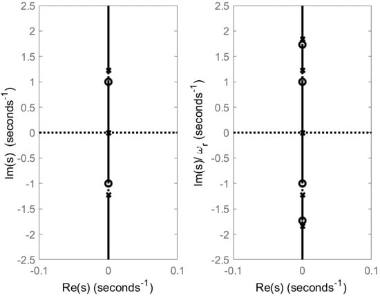
Figure 3. (Left) Conventional metastructure root locus with ${\omega }_m=0.5$, ${\omega }_{2r-1}={\omega }_r=1$, $k_r=1$, $m_r=1$, and $\mu =0.5$. (Right) Metastructure with internal coupling, showing narrow bandgap with ${\omega }_m=0.5$, ${\omega }_{2r}=1.7$, $\kappa =k_r$, and $\mu =0.5$. Internal coupling’s impact on system dynamics is highlighted by the additional bandgap in the right plot.

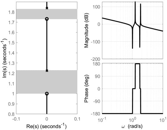
Figure 4. Bode and root locus plots for Equation (34). (Left) Root locus with $K={\omega }_m^2$, showing conventional and internally coupled bandgap for $\mu =0.5$ and $\kappa =1$. Markers: system poles at ${\omega }_m^2=0$, solid lines: pole trajectory as ${\omega }_m^2$ increases. Grey region: bandgap frequency range. (Right) Bode plot showing frequency response, including resonance from coupling effect.

As mentioned earlier, the introduction of $\kappa$ in the coupled system leads to additional zeros and poles, as evidenced by the second root locus in Figure 4. This modification is characterized by the resonant frequencies ${\omega }_{2r-1}=1(\mathrm{rad}/\mathrm{s})$ and ${\omega }_{2r}=1.7(\mathrm{rad}/\mathrm{s})$, suggesting the emergence of a second bandgap. Moreover, the root locus plot in Figure 4 (left) indicates that the internal coupling parameter influences the system’s pole trajectories. Conversely, the Bode plot (right) reveals a pronounced resonant peak, suggesting an increased selective sensitivity to certain frequencies. While the phase response indicates the overall system’s stability under the new coupling condition, it must be carefully evaluated to ensure robustness, especially in control applications where stability is critical.

Dispersion Analysis and Model Validation of Internally Coupled Resonators by Plane Wave Expansion Method

The plane wave expansion (PWE) method is commonly used for analyzing the propagation of waves in periodic structures, and provides valuable insights into the behavior of these waves, facilitating the design and optimization of these periodic structures for a wide range of applications, such as vibration suppression and energy harvesting [12,13].

The transverse displacement of a metastructure with linearly internally coupled resonators in absolute coordinates is defined as $W_t(x,t)={\widehat{W}}_t{e}^{i\left(G_{n}x-\omega t\right)}$ for the beam, $z_{2r-1}\left(t\right)={\widehat{z}}_{2r-1}{e}^{i\left(\omega t\right)}$ for the first resonator, and $z_{2r}\left(t\right)={\widehat{z}}_{2r}{e}^{i\left(\omega t\right)}$ for the second resonator. The dispersion relation emerges from applying periodic boundary conditions to find nontrivial solutions. The relationship between frequency $\omega$ and wavevector $G_n$ in one-directional transformation is established by multiplying the variable’s amplitude with $exp\left(i\left(G_{n}x-\omega t\right)\right)$. With both $k_{r_1}=k_{r_2}=k_r$ and $m_{r_1}=m_{r_2}=m_r$, the equation simplifies as follows:

$$C_1{\omega }^6+C_2{\omega }^4+C_3{\omega }^2+C_4=0$$

(35)

where:

$$\begin{array}{cc}\hfill C_1& =-A{m}_r^2\rho ,\hfill \\ \hfill C_2& =m_r^2\left(EI{G}_n^4+2k_r\right)+2A\rho m_r\kappa +2A\rho m_r{k}_r,\hfill \\ \hfill C_3& =-\left(2\kappa m_r{k}_r+A\rho k_r^2+2A\rho \kappa k_r+EI{G}_n^4{m}_r^2\left(\kappa +2k_r\right)\right),\hfill \\ \hfill C_4& =EI{G}_n^4\left(2\kappa k_r+k_r^2\right).\hfill \end{array}$$

(36)

3. Results and Discussion

The rectangular beam under investigation has the following dimensions: a length of 0.91 m ($L_m$), a width of 40 mm ($w_m$), and a height of 3 mm ($h_m$). The material used for the beam has a density of 2710 km per cubic meter (${\rho }_m$) and a modulus of elasticity of 52 GPa ($E_m$). The beam is characterized by a damping ratio of 0.03 (${\zeta }_m$), and the analysis considers a total of eight vibration modes ($N_m$). Each resonator ($N_r$) within the system has a mass of 80 g ($m_r$) and a spring constant of 380 kilonewtons per meter ($k_r$). The damping ratio for the resonators is also set at 0.03 (${\zeta }_r$).

Figure 5 depicts the dispersion curve of the internally coupled metamaterial beam ($\kappa =k_r$) using the plane wave expansion method. The target frequency corresponds to the resonator frequency. The diagram illustrates two bandgaps: the first is associated with the in-plane behavior of both resonators within each unit cell, while the second bandgap emerges due to the out-of-plane behavior of the two resonators in each unit cell. Here, $G_n$ represents the wave vector number and a denotes the lattice size.

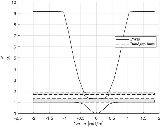
Figure 5. Dispersion curve of an internally coupled metamaterial beam, displaying two distinct bandgaps resulting from in-plane and out-of-plane resonator behavior.

Figure 6 illustrates the transmittance characteristics of a metamaterial beam with internal resonator coupling in terms of tip displacement relative to the base displacement in absolute coordinates. The presence of a common initial bandgap aligns with the theoretical expectations discussed earlier, assuming that all resonators resonate at the same frequency (${\omega }_{2r-1}={\omega }_{2r}={\omega }_r$) and maintain identical phase relationships. In the case of the internally coupled metastructure, an additional bandgap is observed, which substantiates the theoretical premise that variations in resonator frequencies or phase differences can extend the parameter $\kappa$. This extension, facilitated by the assumption of a massless coupling spring, introduces new dynamics to the system by adding an extra pole and zero, resulting in the creation of an additional bandgap. The primary bandgap occurs at the target frequency, which corresponds to the resonator’s frequency adjusted by the length factor $\sqrt{1+\mu }$. The secondary bandgap’s location is contingent upon the stiffness of the internal coupling and is defined by the length factor $\sqrt{1+\frac{\mu }{4}}$. Notably, the dips in the graph signify areas of low transmittance, indicating reduced vibration at the beam’s tip and effectively marking the bandgap regions.

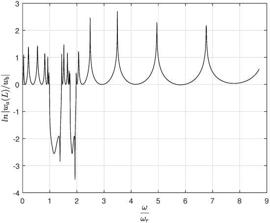
Figure 6. Transmittance plot for a metamaterial beam with internal resonator coupling ($k=k_r$) comprising eight resonators, which equates to four unit cells.

Figure 7 presents a graphical analysis illustrating the influence of varying internal coupling spring constant values, denoted as $\kappa$, on the bandgap frequencies within a metastructure. Notably, alterations in $\kappa$ do not induce substantial shifts in the frequency edges of the primary first bandgap. However, as $\kappa$ increases, it introduces additional, narrower gaps at frequencies above the rest of the second bandgap. These narrower gaps underscore the sensitivity of the metastructure’s dynamic response to specific ranges of internal coupling strength.

Figure 7. Analysis of the influence of internal coupling stiffness $\kappa$ on the metastructure’s bandgap frequencies in Equation (33), showing the consistent edge of the first bandgap and the emergence of narrow higher-frequency gaps within certain $\kappa$ ranges.

Figure 8 presents a contour plot of the transmittance across the metastructure as a function of the normalized internal coupling strength, $\kappa /{\omega }_r$, and normalized frequency, $\omega /{\omega }_r$. The color gradient represents the logarithmic scale of transmittance, indicating the level of wave attenuation within the metastructure. Dark regions correspond to high attenuation levels, signifying the presence of bandgaps. As observed, the contour lines delineate the boundaries of the bandgaps, which become more distinct with specific values of internal coupling strength. This visualization provides a comprehensive understanding of how internal coupling affects the bandgap frequencies, offering insights into the precise tuning of the metastructure’s vibrational properties. It can be seen that the emergence of additional bandgaps occurs within certain ranges of $\kappa$, demonstrating the metastructure’s sensitivity to variations in internal coupling. The plot serves as a detailed map for predicting the dynamic behavior of the metastructure under varying conditions of internal coupling, which is critical for applications requiring targeted vibration isolation frequencies.

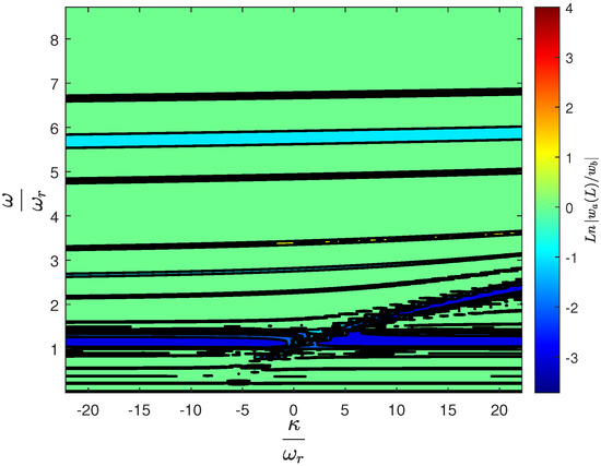
Figure 8. Transmittance contour plot against normalized internal coupling strength and frequency, highlighting bandgap boundaries and the metastructure’s sensitivity to $\kappa$ variations.

The results reveal that metastructures with internally coupled resonators retain the primary bandgap found in conventional metastructures but also introduce an additional, thinner bandgap at a higher frequency. This secondary bandgap remains separate from the primary one, making it challenging to use internal coupling to merge both bandgaps for vibration isolation in continuous and distributed metastructures. This difficulty arises because the second bandgap’s nature is linked to a 180-degree phase change in resonators with identical natural frequencies $\left({\omega }_r\right)$. It would be beneficial to investigate the impact of varying ${\omega }_r$ in different unit cells. Despite these challenges, it is noteworthy that in lumped systems, metastructures with internally coupled resonators significantly widen the bandgap compared to conventional configurations.

4. Finite Element Study

The dynamic behavior of metastructures incorporating internally coupled resonators is investigated using finite element method (FEM) simulations, affirming theoretical predictions. The analysis outputs present the vibrational modes of the metastructure. These modes are expressed as amplitude variations across a spectrum of normalized frequencies, with a particular focus on resonant frequencies pertinent to bandgap development. Significant findings from the analysis illustrate the variance in bandgap distribution and intensity of resonant peaks as a function of stiffness ratio. This implies a substantial relationship between internal coupling stiffness and the dynamic response of the metastructure. Visualization of these results not only confirms primary and secondary bandgap presence but also aligns with the theoretical implications of internal resonator coupling. Figure 9 concentrates on the transmissibility for a specific stiffness ratio $\kappa$, reflecting a critical scenario where $\kappa$ is precisely matched with the resonator’s stiffness $\left(\kappa /{\omega }_r=0.003\right)$, an essential condition for optimal bandgap definition. This particular observation underscores the necessity of accurate internal coupling stiffness to achieve the designed dynamic response.

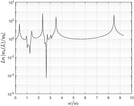
Figure 9. Transmissibility for a cantilever beam with stiffness ratio $\kappa$ equal to $k_r$, demonstrating optimal internal coupling for bandgap clarity.

However, deviations from the ideal $\kappa$ value lead to pronounced disorder within the system’s response, emphasizing the metastructure’s sensitivity to variations in internal coupling stiffness. Such irregularities pose challenges for ensuring predictability and consistent performance in practical applications, thus advocating for stringent precision in design and manufacturing processes.

The contour plot depicted in Figure 10 utilizes a binary representation to mark regions of transmittance reduction, set at $log\left({10}^{-0.1}\right)$. The provided binary representation displays two distinct white regions against a cyan background, illustrating the transmittance levels across various stiffness ratios $\kappa$ and normalized frequencies. The first white region, located at the target resonator frequency ${\omega }_r$, corresponds to a bandgap typically observed in conventional metamaterials. This bandgap represents a frequency range where the structure prevents wave propagation, thereby indicating a strong vibration isolation capability at the resonant frequency of the metamaterial. The second white region appears at a higher frequency range and signifies the impact of internal coupling within the metamaterial structure. This additional bandgap is a result of the specific design and internal resonator interactions that are a characteristic of the studied metastructures. The emergence of this second bandgap highlights the effect of internal coupling on the extension of vibration isolation performance to higher frequency ranges.

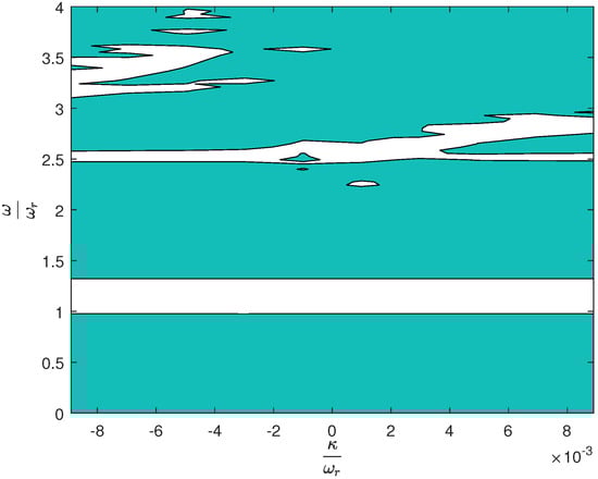
Figure 10. Binary contour plot illustrating the presence and absence of transmittance corresponding to bandgaps as a function of stiffness ratio $\kappa$ and normalized frequency.

Impact of Spacial Variations on Bandgap Characteristics

The established methodology enables manipulation of the transfer function, thereby permitting exploration into how adjustments in the mass placement on a resonator affect bandgap traits, a key factor for refining bandgap properties within a closed-loop control system.

This section explores adjusting resonator stiffness while maintaining constant mass, a method beneficial for heavy machinery applications where traditional piezoelectric solutions may fall short. Stiffness tuning, as opposed to piezoelectric adjustments, offers a more durable and practical solution for these demanding environments. The current study examines a conventional metastructure that does not incorporate internally coupled resonators. The resonators are of the cantilever type, with a mass that can be positioned along the length from the tip to the base. The specific parameters defining the metastructure and resonators are as follows: eight resonators ($N_r=8$), with the beam dimensions being 300 mm in length, 25 mm in width, and 3 mm in height. The material density is 2700 kg/m³, and the modulus of elasticity is 69.5 GPa. The damping ratio of the structure and resonators is the same, at 0.01. An attached mass ($m_a$) of 3.8 g is placed at distances that vary from 20 to 57.3 mm along the resonator. The natural frequency of the resonator (${\omega }_r$), when the attached mass is at the tip, is 32 Hz. This setup allows for an exploration of the resonator stiffness’s impact on the bandgap properties of the metastructure.

Figure 11 provides a 3D visualization of how the position of the attached mass along the length of a resonator affects the bandgap frequencies in a metastructure. The natural frequency at which the bandgap starts is denoted as ${\omega }_r$, corresponding to the case when the mass is located at the tip of the resonator. The graph demonstrates that as the mass moves closer to the base of the resonator—decreasing $\delta$—the resonator’s stiffness increases, leading to a rise in ${\omega }_r$ and a subsequent shift of the bandgap towards higher frequencies.

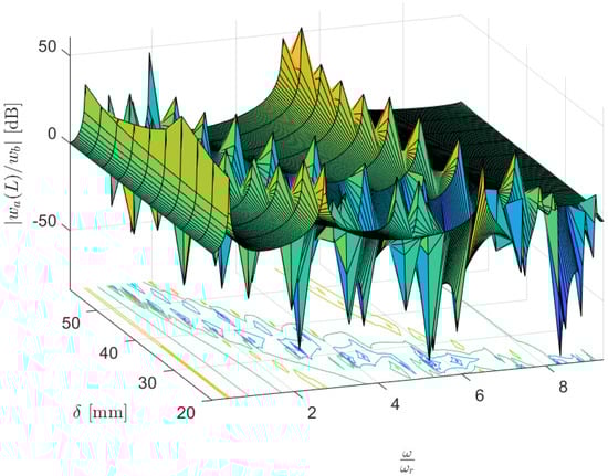
Figure 11. A 3D plot showing the shift in bandgap frequency related to mass positioning on the resonator, with delta $\left(\delta \right)$ representing the mass location from the resonator’s tip to base.

The contour plot in the x–y plane clearly depicts the bandgap’s initiation at the initial natural frequency ${\omega }_r$ when the mass is at the resonator’s tip. From there, the bandgap expands and moves as the location of the mass changes. This shift is particularly crucial for applications requiring tunable vibration isolation, as it shows the potential to adjust the bandgap frequency by simply repositioning the resonator mass without altering the resonator or structure itself.

The binary representation in Figure 12 illustrates the influence of the mass location along the resonator on the bandgap frequencies. With the bandgap depth limit set at a decibel ratio of output to input displacement of 0.2, the plot shows that when the attached mass is positioned at the tip of the resonator, the bandgap originates at the resonator frequency ${\omega }_r$. The white areas in the binary representation correlate to the regions of significant transmittance reduction, effectively mapping the bandgap’s presence and evolution as the mass moves closer to the resonator’s base.

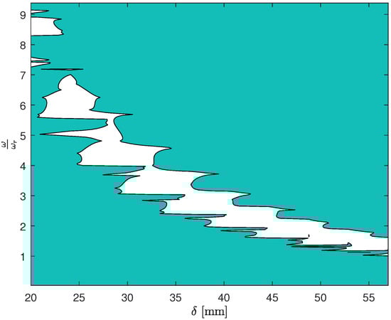
Figure 12. Binary contour plot of bandgap presence against resonator mass placement ($\delta$) and normalized frequency ($\omega /{\omega }_r$), with white areas indicating effective vibration isolation regions.

5. Conclusions

This study explored the dynamic behavior of metastructures, focusing on those with conventional configurations and those augmented with internally coupled resonators, through a theoretical lens. The development of analytical models deepened our understanding of bandgap dynamics, highlighting the prediction of primary and secondary bandgaps as influenced by internal coupling stiffness. Finite element analysis (FEA) corroborated these theoretical insights, yet it also exposed complexities beyond the analytical models’ scope. Insights gained from this study stress the importance of accurately accounting for the physical characteristics of internal couplings and achieving exact stiffness ratios. Additionally, this work shows that adjusting the natural frequencies of resonators through stiffness manipulation—via the strategic positioning of mounted masses—provides a viable approach for customizing vibration isolation solutions. This strategy is particularly relevant for environments subjected to heavy loads and extreme conditions, offering tailored responses to complex vibrational challenges.

The principal contributions of this research are as follows:

• We established a novel transfer function approach for the analysis of metastructures, diverging from traditional bandgap investigation methods such as dispersion analysis and wave finite element methods.
• We applied root locus analysis and transfer function modeling, offering new perspectives on metastructure control.
• We demonstrated the enhanced dynamic bandgap characteristics achievable through the use of internally coupled resonators, incorporating control engineering techniques for refined metastructure management.

This research showcases the fusion of control system theory with metastructure analysis, presenting a groundbreaking approach for the precise manipulation of bandgaps. This methodology not only marks a significant advancement in the understanding and application of vibration control technologies but also opens new avenues for energy-efficient solutions across multiple industries. Specifically, in the automotive sector, the integration of metastructures can significantly reduce noise and vibrations, enhancing vehicle durability. In civil engineering, buildings and infrastructure equipped with optimized bandgaps offer enhanced protection against environmental vibrations and seismic activities. Moreover, the innovative application of these metastructures in energy harvesting from vibrational bandgaps paves the way for smart buildings to achieve superior energy sustainability.

Future studies will prioritize empirical validation through experimentation to confirm the theoretical and numerical models’ applicability in real-world scenarios. Subsequent research will focus on fabricating metastructures with internally coupled resonators, with a particular emphasis on manufacturing precision to accurately match the stiffness of the resonators, thereby ensuring optimal system performance. Additionally, the integration of piezoelectric materials for vibration suppression and energy harvesting will be explored, aiming to enhance the functional versatility of these advanced materials.

References

- Shelby, R.A.; Smith, D.R.; Schultz, S. Experimental verification of a negative index of refraction. Science 2001, 292, 77–79. [Google Scholar] [CrossRef] [PubMed]
- Liu, Z.; Zhang, X.; Mao, Y.; Zhu, Y.; Yang, Z.; Chan, C.T.; Sheng, P. Locally resonant sonic materials. Science 2000, 289, 1734–1736. [Google Scholar] [CrossRef] [PubMed]
- Hazra, S.; Bhattacharjee, A.; Chand, M.; Salunkhe, K.V.; Gopalakrishnan, S.; Patankar, M.P.; Vijay, R. Ring-resonator-based coupling architecture for enhanced connectivity in a superconducting multiqubit network. Phys. Rev. Appl. 2021, 16, 024018. [Google Scholar] [CrossRef]
- Rozenman, G.G.; Peisakhov, A.; Zadok, N. Dispersion of organic exciton polaritons—A novel undergraduate experiment. Eur. J. Phys. 2022, 43, 035301. [Google Scholar] [CrossRef]
- Li, Y.; Yefremenko, V.G.; Lisovenko, M.; Trevillian, C.; Polakovic, T.; Cecil, T.W.; Barry, P.S.; Pearson, J.; Divan, R.; Tyberkevych, V.; et al. Coherent coupling of two remote magnonic resonators mediated by superconducting circuits. Phys. Rev. Lett. 2022, 128, 047701. [Google Scholar] [CrossRef]
- Hu, G.; Tang, L.; Das, R. Internally coupled metamaterial beam for simultaneous vibration suppression and low frequency energy harvesting. J. Appl. Phys. 2018, 123, 055107. [Google Scholar] [CrossRef]
- Oyelade, A.O.; Oladimeji, O.J. Coupled multiresonators acoustic metamaterial for vibration suppression in civil engineering structures. Forces Mech. 2021, 5, 100052. [Google Scholar] [CrossRef]
- Erturk, A.; Inman, D.J. A distributed parameter electromechanical model for cantilevered piezoelectric energy harvesters. J. Vib. Acoust. 2008, 130, 041002. [Google Scholar] [CrossRef]
- Sugino, C.; Xia, Y.; Leadenham, S.; Ruzzene, M.; Erturk, A. A general theory for bandgap estimation in locally resonant metastructures. J. Sound Vib. 2017, 406, 104–123. [Google Scholar] [CrossRef]
- Hansen, C.; Snyder, S.; Qiu, X.; Brooks, L.; Moreau, D. Active Control of Noise and Vibration; CRC Press: Boca Raton, FL, USA, 2012. [Google Scholar]
- Meirovitch, L. Fundamentals of Vibrations; Waveland Press: Long Grove, IL, USA, 2010. [Google Scholar]
- Li, F.L.; Zhang, C.; Wang, Y.S. Band structure analysis of phononic crystals with imperfect interface layers by the BEM. Eng. Anal. Bound. Elem. 2021, 131, 240–257. [Google Scholar] [CrossRef]
- Lei, L.; Miao, L.; Zheng, H.; Wu, P.; Lu, M. Band gap extending of locally resonant phononic crystal with outward hierarchical structure. Appl. Phys. A 2022, 128, 492. [Google Scholar] [CrossRef]
- Rao, S.S. Vibration of Continuous Systems; John Wiley & Sons: Hoboken, NJ, USA, 2019. [Google Scholar]
Disclaimer/Publisher’s Note: The statements, opinions and data contained in all publications are solely those of the individual author(s) and contributor(s) and not of MDPI and/or the editor(s). MDPI and/or the editor(s) disclaim responsibility for any injury to people or property resulting from any ideas, methods, instructions or products referred to in the content. |
© 2024 by the authors. Licensee MDPI, Basel, Switzerland. This article is an open access article distributed under the terms and conditions of the Creative Commons Attribution (CC BY) license (https://creativecommons.org/licenses/by/4.0/).