Optimal Opacity-Enforcing Supervisory Control of Discrete Event Systems on Choosing Cost

Abstract

To ensure opacity, it is optimal to retain as many as possible occurring event sequences. Contrary to this problem, the other optimal goal is to preserve the minimal occurring event sequences. Based on the choosing cost, an optimal opacity-enforcing problem with minimal discount choosing cost is presented under two constraints in this paper. The first constraint is the opacity of the controlled system. The second is the retention of the secret to the maximum. To solve the model, two scenarios on opacity are considered. For the two scenarios, some algorithms are presented to achieve the optimal solution for the model by using the method of dynamic programming. Then, the solutions produced by the algorithms are proved to be correct by theoretical proof. Finally, some illustrations and an application example on location privacy protection for the algorithms are given.

1. Introduction

In modern society, when important information about enterprises is released online, it generally needs to be as complete as possible. In order to keep the security and opacity of important data transmission, it is necessary to use some unimportant data to confuse and make it difficult to distinguish from an adversary. The more information is used to confuse important data, the better it is. Therefore, some papers (e.g., [1,2,3,4]) discussed the issue of maximum opaque sublanguages. However, in reality, due to the cost involved in using data transmission, less unimportant data and lower transmission costs are preferred. Therefore, this paper proposes an optimization mathematical model to find the most cost-effective information to confuse the important data to be released and proposes an algorithm to obtain the optimal control strategy.

In 2004, opacity was first introduced to analyze cryptographic protocols in [5]. In 2005, the research modeled as Petri nets in [6] brought opacity to the field of discrete event systems (DES). Afterward, the research on opacity in DES boomed up. In DES models, the definition of opacity was divided into two cases: language-based opacity [1,7,8] (e.g., strong opacity [7], weak opacity [7], non-opacity [7]) and state-based opacity [6,9,10,11,12,13] (e.g., current-state opacity [6,9], initial-state opacity [6], initial-and-final-state opacity [13], K-step opacity [9,10,11], infinite-step opacity [12,14]). In ref. [15], the works of [13] were extended, and it was shown that the various notions of opacity can be transformable to each other. Then, in Ref. [16], the existing notions of opacity were unified and a general framework was provided. With the definition of opacity, the verification approach was investigated in the previous works. Once a system was not opaque, supervisory control theory [1,4,17] or the enforcement approach [18,19,20,21,22] were presented to ensure opacity in the system. In general, supervisory control theory restricts the behavior of the system to ensure opacity, whereas the enforcement approach does not restrict but modifies the output of the system to ensure opacity. For example, in Ref. [1], fix-point theory was used to check the opacity of the closed system at every iteration to achieve the maximal permissive supervisor on condensed state estimates. In Ref. [4], the maximal permissive supervisor was obtained using the refining of the plant and observer instead of condensed state estimates. In Ref. [17], strong infinite- and k-step opacity was transformed into a language and an algorithm was presented to enforce infinite- and k-step opacity by a supervisor. In Ref. [18], the synthesis of insertion function was extended from current-state opacity [23] to infinite-step opacity and K-step opacity. In Ref. [19], fictitious events were inserted at the output of the systems to enforce the opacity of the system. And some works [20,21] extended the method of [19], where the authors of Ref. [20] discussed the problem of opacity enforcement under energy constraints and the authors of Ref. [21] studied supervisory control under local mean payoff constraints. In Ref. [22], current-state opacity was verified and enforced based on an algebraic state space approach for partially observed finite automaton.

To ensure opacity, in Ref. [24], some algorithms were proposed to design a controller to control information released to the public. And then, in Ref. [25], the work of [24] was extended, and then an algorithm was presented for finding minimal information release policies for non-opacity. In Ref. [26], a reward was assigned for revealing the information of each transition and the maximum guaranteed payoff policy was found for the weighted DES. In Ref. [27], a dynamic information release mechanism was proposed to verify current-state opacity where information is partially released and state-dependent.

To ensure opacity, the secret is preserved by enabling/disabling some events to restrict the behavior of the system. If cost functions are defined in DES, two types of optimal supervisory control problems are developed: one is for event cost, and the other is for control cost. For example, in Ref. [28], the cost of events was defined to design a supervisor to minimize the total cost to reach the desired states. Then, in Ref. [29], the framework was extended to the partial observation of the system. Afterward, in Ref. [30], the mean payoff supervisory control problem was investigated for a system where each event has an integer associated with it. In [31,32], the costs of choosing control input and occurring event were defined and two optimal problems to minimize the maximal discounted total cost among all possible strings generated in the systems were solved using Markov decision processes.

In contrast to the supremal opaque sublanguage of the plant in [1,2,3,4,8], we want to find a ‘smallest’ closed controllable sublanguage of the plant, concerning which the secret is not only opaque but also ‘largest’. Since the class of opaque languages is not closed under intersection [8], ‘smallest’ does not refer to set inclusion, but to minimal discount total choosing cost. On the other hand, ‘largest’ refers to set inclusion, where it means the union of all the elements of the class of confused secret. To describe the optimal problem, a non-linear optimal supervisory control model is proposed by introducing the concept of choosing cost.

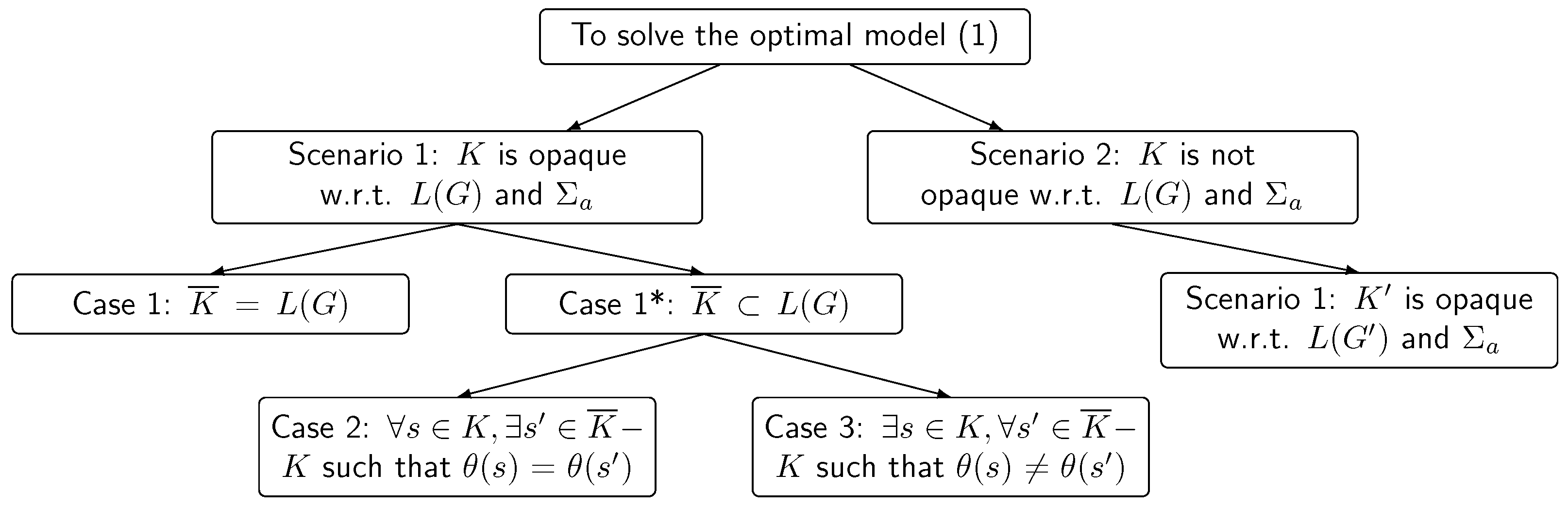
The paper is organized as follows. Section 2 establishes the background on supervisory control theory, opacity, and choosing cost of DES. In Section 3, we present an optimal supervisory control problem that is modeled by non-linear programming with two constraint conditions. In Section 4, we propose two scenarios to show the computational process of the optimal problem. The first scenario is divided into three cases in Section 5, where we suppose that the plant can ensure the secret is opaque, and some algorithms and theorems are put forward to the solution of the optimal problem. In Section 6, a generalized algorithm and theorem are proposed under the second scenario, where the plant cannot ensure the secret is opaque. Finally, the main contribution of the work is discussed in Section 7.

2. Preliminary

2.1. Supervisory Control Theory

We consider a DES modeled by a determined finite transition system, $G=(Q,\Sigma ,\delta ,q_0)$, where Q is a finite set of states, $\Sigma$ is a finite set of events labeled in the transition, partial function $\delta :\Sigma \times Q\to Q$ is the transition function and $q_0\in Q$ is the initial state. A run of G is a finite non-empty sequence, $q_0{\sigma }_1{q}_1{\sigma }_2\cdots q_{n-1}{\sigma }_n$, where $q_i\in Q,{\sigma }_{i+1}\in \Sigma$ and $q_{i+1}=\delta (q_i,{\sigma }_i)$ for $i=1\cdots n-1$. The trace $tr\left(\rho \right)$ of run $\rho$ is ${\sigma }_1{\sigma }_2\cdots {\sigma }_n$. The languages of G are the set of all traces of runs of G, and they are denoted $L\left(G\right)=\{s\in {\Sigma }^{*}|\delta (s,q_0)!\}$. Event set $\Sigma$ is assumed to be partitioned into controllable event set ${\Sigma }_c$ and uncontrollable event set ${\Sigma }_u$, where $\Sigma ={\Sigma }_c\dot{\cup }{\Sigma }_u$. Each subset of events is a control pattern, and the set of all control patterns is denoted by $\Gamma =\left\{\gamma \right|{\Sigma }_u\subseteq \gamma \subseteq \Sigma \}$. A supervisor for G is any map f: $L\left(G\right)\to \Gamma$. For system G, we denote ${\Gamma }^{L\left(G\right)}$ as the set of supervisors. The closed behavior of $f/G$, i.e., G under the supervision of f, is defined to be language $L(f/G)\subseteq L\left(G\right)$ described as follows:

• $ϵ\in L(f/G)$;
• $s\sigma \in L(f/G)\iff s\in L(f/G),s\sigma \in L\left(G\right),\sigma \in f\left(s\right)$.

For language $K\subseteq L\left(G\right)$, notation $\overline{K}$ is said to be the prefix(-closure) of K. K is said to be (prefix-)closed if $\overline{K}=K$.

Definition 1 

([33]). We consider non-empty language K. Then, K is controllable if $\overline{K}{\Sigma }_u\cap L\left(G\right)\subseteq \overline{K}$.

A necessary and sufficient condition for the existence of a supervisor is given as follows:

Theorem 1 

([33]). We consider non-empty language $K\subseteq L\left(G\right)$. Then, there exists supervisor f such that $L(f/G)=K$ if and only if K is a controllable and closed language.

2.2. Supervisory Control for Opacity

Assuming that the adversary can be aware of any supervisor’s control policy, a subset ${\Sigma }_a$ of the events can be seen by the adversary through an observable function, $\theta$: ${\Sigma }^{*}\to {\Sigma }_a^{*}$. An adversary’s observation of the system is denoted by $obs\left(G\right)=\{Q_a,{\Sigma }_a,{\delta }_a,q_{0a}\}$, which is an observer of system G. If an observer of the system is unable to determine some secret information, we offer the following equivalent definitions of opacity:

Definition 2 

([1]). We consider system G and non-empty language K. For any $s\in K\cap L\left(G\right)$, if there exists $s^{\prime }\in L\left(G\right)-K$ such that $\theta \left(s\right)=\theta \left(s^{\prime }\right)$, we say K is (strongly) opaque with respect to $L\left(G\right)$ and ${\Sigma }_a$.

Definition 3 

([7]). We consider system G and non-empty language K. K is strongly opaque with respect to $L\left(G\right)$ and θ if $\theta \left(K\right)\subseteq \theta \left(L\right(G)-K)$.

If the condition of Definition 2 cannot be met, we say K is not (strongly) opaque with respect to $L\left(G\right)$ and ${\Sigma }_a$. For the definition of non-opacity, it is different from that of [7].

In [8], since opaque language has a desirable property that it is closed under union, there exist supremal controllable closed and opaque sublanguages of the system [1,4]. In [1,4,8], different works about supremal controllable closed and opaque sublanguage are computed.

2.3. The Definition of Choosing Cost

In [31,32], two optimal control models of DES are presented based on the costs of choosing a control input and an event occurring, respectively. In this paper, the choosing cost is obtained from the definition of the cost of choosing the control input after some string of [31,32]. For a given DES G, we let $c(s,\gamma )$ be the cost of choosing control input $\gamma$ at string s, where $s\in L\left(G\right)$, $\gamma \in \Gamma$ and $c(s,\gamma )$ is nonnegative. For any supervisor f: $L\left(G\right)\to \Gamma$, we call $c(s,f)=c(s,f(s\left)\right)$ the cost of choosing $f\left(s\right)$ after s under the supervision of f. All in all, we simply call $c(s,\gamma )$ (or $c(s,f)$) the choosing cost.

3. Optimal Supervisory Control Model on Opacity

In the section, an optimal supervisory control model is constructed to minimize the choosing cost of the controlled system which is opaque. Given system G and secret $K\subseteq L\left(G\right)$, as shown in [1], secret K is a regular language. For secret K, we suppose there exists a set of secret states $Q_s\subseteq Q$ which can recognize secret K, i.e., $s\in K$ iff $\delta (q_0,s)\in Q_s$.

To show the cost of information released, we introduce the cost of choosing control input in [31,32] and define the total choosing cost as follows:

Definition 4. 

Given closed-loop behavior $L(f/G)$, the discount total choosing cost of $L(f/G)$ is defined as $V(L(f/G),f)={\displaystyle \sum _{s\in L(f/G)}}{\beta }^{\left|s\right|}c(s,f)$, where f is a supervisor controlling system G and $\beta >0$ is a discount factor. For convenience, $V\left(L\right(f/G),f)$ is simplified as $V\left(L\right(f/G\left)\right)$.

For system G, if there exist two supervisors $f_1$ and $f_2$ such that $L(f_1/G)\subseteq L(f_2/G)$, it is obvious that $V\left(L(f_1/G)\right)\le V\left(L(f_2/G)\right)$ by Definition 4.

To obtain the discount total choosing cost, we definite discount cost by the sum of choosing cost after s under f.

Definition 5. 

We consider s, $t_n={\sigma }_1{\sigma }_2\cdots {\sigma }_n$ and $t_k={\sigma }_1{\sigma }_2\cdots {\sigma }_k(0\le k\le n,t_0=ϵ)$. Then, $V_s\left(t_n\right)={\displaystyle \sum _{k=0}^n}{\beta }^{\left|s\right|+k}c(s{t}_k,f_{s{t}_n})$ is said to be the discount cost of choosing $t_n$ after s under f, where $f_{s{t}_n}\left(s{t}_k\right)=f\left(s{t}_k\right)\cap {\Sigma }_{s{t}_n}\left(s{t}_k\right)$ and ${\Sigma }_{s{t}_n}\left(s{t}_k\right)=\left\{\sigma \right|s{t}_k\sigma \in \overline{s{t}_n}\}$. Particularly, if $k=0$, i.e., $t_0=ϵ$, then $V_s\left(ϵ\right)={\beta }^{\left|s\right|}c(s,\varphi )=0$; if $s=ϵ$, then $s{t}_n=t_n$ and $V_{ϵ}\left(t_n\right)={\displaystyle \sum _{k=0}^n}{\beta }^{k}c(t_k,f_{t_n})$, where $t_0=ϵ$ means that choosing $f\left(s\right)$ at s has nothing to do with Σ.

In Definition 5, if some string can be divided into two pieces, a formula is formulated to simplify the computation of discount cost in the following conclusions:

Proposition 1. 

We consider $t=s{t}^{\prime }$. Then, we have $V_{ϵ}\left(t\right)=V_{ϵ}\left(s\right)+V_s\left(t^{\prime }\right)$.

Proof. 

For $t=s{t}^{\prime }$, we proved the following formula, where $s={\sigma }_1{\sigma }_2\cdots {\sigma }_{\left|s\right|}$ and $t^{\prime }={\sigma }_{\left|s\right|+1}{\sigma }_{\left|s\right|+2}\cdots {\sigma }_{\left|s\right|+n}$:

$$\begin{array}{ccc}\hfill V_{ϵ}\left(t\right)& & =\sum _{k=0}^{\left|s\right|+n}{\beta }^{k}c(t_k,f_t)\hfill \\ & & =c(ϵ,f_s)+\beta c({\sigma }_1,f_s)+\cdots +{\beta }^{\left|s\right|}c(s,f_s)+\sum _{k=1}^n{\beta }^{\left|s\right|+k}c(s{t}_k^{\prime },f_{s{t}^{\prime }})\hfill \\ & & =\sum _{k=0}^{\left|s\right|}{\beta }^{k}c({\sigma }_1\cdots {\sigma }_k,f_s)+\sum _{k=0}^n{\beta }^{\left|s\right|+k}c(s{t}_k^{\prime },f_{s{t}^{\prime }})\hfill \\ & & =V_{ϵ}\left(s\right)+V_s\left(t^{\prime }\right)\hfill \end{array}$$

  □

To generalize the above Proposition 1, we have the following conclusion as Proposition 2:

Proposition 2. 

We consider $s=s_1{s}_2\cdots s_k\in L\left(G\right)$. Then, we have $V_{ϵ}\left(s\right)=V_{ϵ}\left(s_1\right)+V_{s_1}\left(s_2\right)+\cdots +V_{s_1{s}_2\cdots s_{k-1}}\left(s_k\right)$.

Proof. 

The proof can proceed by induction.

Base case: If $k=1$, then it holds that $V_{ϵ}\left(s\right)=V_{ϵ}\left(s_1\right)$.

Inductive hypothesis: Suppose that we have $V_{ϵ}(s_1\cdots s_{j-1}{s}_j)=V_{ϵ}\left(s_1\right)+V_{s_1}\left(s_2\right)+\cdots +V_{s_1{s}_2\cdots s_{j-1}}\left(s_j\right)$ if $k=j$.

Inductive step: For $k=j+1$, we prove that $V_{ϵ}(s_1\cdots s_{j-1}{s}_j{s}_{j+1})=V_{ϵ}\left(s_1\right)+V_{s_1}\left(s_2\right)+\cdots +V_{s_1{s}_2\cdots s_{j-1}}\left(s_j\right)+V_{s_1{s}_2\cdots s_j}\left(s_{j+1}\right)$.

By Definition 5, we have the following, which completes the inductive step:

$$\begin{array}{ccc}\hfill V_{ϵ}\left(s\right)& & =V_{ϵ}(s_1\cdots s_{j-1}{s}_j{s}_{j+1})\hfill \\ & & =V_{ϵ}(s_1\cdots s_{j-1}{s}_j)+V_{s_1\cdots s_{j-1}{s}_j}\left(s_{j+1}\right)\hfill \\ & & (\because \mathrm{Proposition} 1)\hfill \\ & & =V_{ϵ}\left(s_1\right)+V_{s_1}\left(s_2\right)+\cdots +V_{s_1{s}_2\cdots s_{j-1}}\left(s_j\right)+V_{s_1\cdots s_{j-1}{s}_j}\left(s_{j+1}\right)\hfill \\ & & (\because \mathrm{Hypothesis}k=j)\hfill \end{array}$$

  □

To obtain the discount total choosing cost, we formulate Algorithm 1 to obtain $V\left(L\right(f/G\left)\right)$ by the computation of $V_s\left(s^{\prime }\right)$.

Algorithm 1 Computing $V\left(L\right(f/G\left)\right)$, the discount total choosing cost of $L(f/G)$

Input: $L(f/G)$; Output: $V\left(L\right(f/G\left)\right)$.  1: Let root = $q_0$.  2: Let $Q_v=Q$.  3: for $q\in Q-\left\{q_0\right\}$do  4:   Compute the in-degree of state q.  5:   if in-degree of state q is more than 1 then  6:    Copy state q and its successor states and traces based on its in-degree.  7:    Insert the states q and its successor into Q and $Q_v$.  8:   end if  9: end for   10: for $q\in Q-\left\{q_0\right\}$do   11:   Compute the out-degree of state q.   12:   if out-degree =1 then   13:    Concatenate the transitions from q’s parent to q’s child via q, i.e., achieve a transition ($q’\mathrm{s}\mathrm{parent}\stackrel{ab}{\to }q’\mathrm{child}$) from the transitions ($q’\mathrm{s}\mathrm{parent}\stackrel{a}{\to }q$ and $q\stackrel{b}{\to }q’\mathrm{s}\mathrm{child}$).   14:    $Q=Q-\left\{q\right\}$   15:   end if   16: end for   17: At some node q, if there exists a transition s from root to q and a transition $s^{\prime }$ from q to its child (i.e., root $\stackrel{s}{\to }q\stackrel{s^{\prime }}{\to }q$’s child), we have $V_s\left(s^{\prime }\right)$.   18: By breadth-first search, we traverse all the nodes and have $V\left(L(f/G)\right)={\displaystyle \sum _{q\in Q_v}}{V}_s\left(s^{\prime }\right)$   19: return $V\left(L\right(f/G\left)\right)$

As shown in Algorithm 1, closed-system $f/G$ can be transformed into a tree automaton, where the closed-system is language-equivalent with the tree automaton. To obtain the longest common prefix of some strings, we need to compute the out-degree of each node. In the tree automaton, if the out-degree of some node is greater than one, the string from the root to the node must be the longest common prefix of some strings from the root to the leaves via the node.

To show the computational process of Algorithm 1, an example is given to obtain the discount total choosing cost.

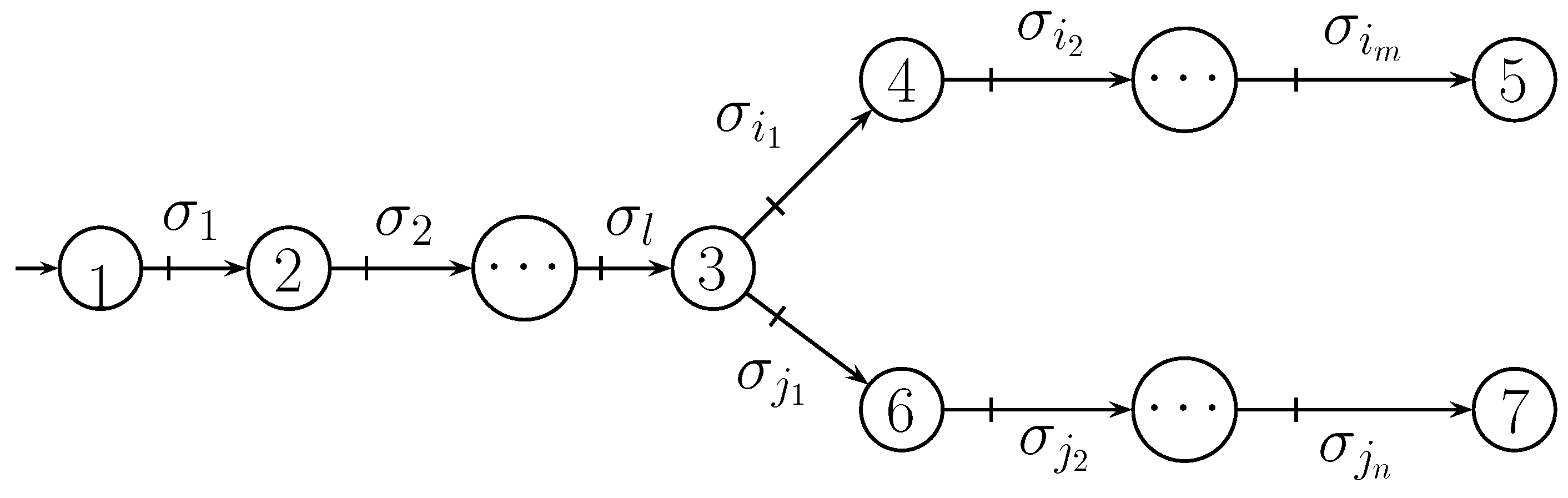
Example 1. 

Suppose that $L(f/G)=\{\overline{s_1},\overline{s_2}\}$ and t is the longest common prefix of $s_1$ and $s_2$. To simplify the process of computation in Definition 4, we denote $t={\sigma }_1\cdots {\sigma }_l,t_1={\sigma }_{i_1}\cdots {\sigma }_{i_m}$ and $t_2={\sigma }_{j_1}\cdots {\sigma }_{j_n}$ such that $s_1=t{t}_1$ and $s_2=t{t}_2$. By Definition 4, we have the following equation:  

$$\begin{array}{ccc}\hfill V\left(\{\overline{s_1},\overline{s_2}\}\right)& =& \sum _{k=0}^l{\beta }^{k}c({\sigma }_1\cdots {\sigma }_k,f_{{\sigma }_1\cdots {\sigma }_l})+{\beta }^l\sum _{k=0}^m{\beta }^{k}c({\sigma }_1\cdots {\sigma }_l{\sigma }_{i_1}\cdots {\sigma }_{i_k},f_{{\sigma }_1\cdots {\sigma }_l{\sigma }_{i_1}\cdots {\sigma }_{i_m}})\hfill \\ & & +{\beta }^l\sum _{k=0}^n{\beta }^{k}c({\sigma }_1\cdots {\sigma }_l{\sigma }_{j_1}\cdots {\sigma }_{j_k},f_{{\sigma }_1\cdots {\sigma }_l{\sigma }_{j_1}\cdots {\sigma }_{j_n}})\hfill \\ & =& V_{ϵ}\left(t\right)+V_t\left(t_1\right)+V_t\left(t_2\right)\hfill \\ & =& V_{ϵ}\left(t{t}_1\right)+V_t\left(t_2\right)\hfill \\ & =& V_{ϵ}\left(s_1\right)+V_t\left(t_2\right)\hfill \\ & =& V_{ϵ}\left(s_2\right)+V_t\left(t_1\right)\hfill \end{array}$$

According to Algorithm 1, we transform $L(f/G)$ in Figure 1 into a tree automaton shown in Figure 2.

By Figure 2 and Algorithm 1, we have the following formula:

$$\begin{array}{ccc}\hfill V\left(\{\overline{s_1},\overline{s_2}\}\right)& =& V_{ϵ}\left(t\right)+V_t\left(t_1\right)+V_t\left(t_2\right)\hfill \\ & =& V_{ϵ}\left(t{t}_1\right)+V_t\left(t_2\right)\hfill \\ & =& V_{ϵ}\left(s_1\right)+V_t\left(t_2\right)\hfill \\ & =& V_{ϵ}\left(s_2\right)+V_t\left(t_1\right)\hfill \end{array}$$

If there exists language K such that $\overline{K}\subseteq L(f/G)$, the discount total choosing cost of $\overline{K}$ can be denoted by $V\left(\overline{K}\right)$ and obtained as shown in Algorithm 1. If we denote $V(L(f/G)-\overline{K})$ by $V\left(L(f/g)\right)-V\left(\overline{K}\right)$, we can also obtain the discount cost using Definition 5. $V(L(f/G)-\overline{K})$ means to compute the choosing cost outside of $\overline{K}$ in $L(f/G)$. Next, we continue the above Example 1.

Example 2. 

In Figure 1, we assume there exists state subset $Q_K=\{4,6\}$ such that $K=t({\sigma }_{i1}+{\sigma }_{j1})$. By Algorithm 1, we obtain a tree automaton based on $\overline{K}$ shown in Figure 3. So, it holds that $V\left(\overline{K}\right)=V_{ϵ}\left(t\right)+V_t\left({\sigma }_{i1}\right)+V_t\left({\sigma }_{j1}\right)$. According to the formulas of $V\left(L\right(f/G)$ and $V\left(\overline{K}\right)$, we have the following equation:  

$$\begin{array}{ccc}\hfill V(L(f/G)-\overline{K})& =& [V_{ϵ}\left(t\right)+V_t\left(t_1\right)+V_t\left(t_2\right)]-[V_{ϵ}\left(t\right)+V_t\left({\sigma }_{i1}\right)+V_t\left({\sigma }_{j1}\right)]\hfill \\ & =& V_t\left(t_1\right)-V_t\left({\sigma }_{i1}\right)+V_t\left(t_2\right)-V_t\left({\sigma }_{j1}\right)\hfill \\ & =& V_{t{\sigma }_{i1}}({\sigma }_{i2}\cdots {\sigma }_{im})+V_{t{\sigma }_{j1}}({\sigma }_{j2}\cdots {\sigma }_{jn})\hfill \end{array}$$

For the system and the secret, we propose an optimal problem to synthesize a supervisor such that the discount total choosing cost of the controlled system is minimal.

Optimal opacity-enforcing problem. Given system G and secret $K\subseteq L\left(G\right)$, we find supervisor f such that $L(f/G)$ satisfies the following conditions:

1.

K is opaque with respect to $L(f/G)$ and ${\Sigma }_a$;

2.

All the secret information that has not been leaked in G remains in the closed-loop system $f/G$;

3.

For closed-loop behavior $L(f/G)$, discount total choosing cost $V\left(L\right(f/G\left)\right)$ is minimal.

In Condition 1 of the above problem, if K is opaque with respect to $L(f/G)$ and ${\Sigma }_a$, we have $\theta (K\cap L(f/G\left)\right)\subseteq \theta \left(L\right(f/G)-K)$ by Definition 3.

In Condition 2, if the supremal controllable and closed sublanguage of $L\left(G\right)$ are denoted by $L(g/G)$ [4], the largest secret K permitted by supervisor f is $L(g/G)\cap K$. So, all the secret information that is not leaked in G is $L(g/G)\cap K$. Therefore, the second condition implies that $K\cap L(f/G)=K\cap L(g/G)$ holds.

In Condition 3, we hope that objective function $V\left(L\right(f/G\left)\right)$ is minimal.

Based on the above optimal problem and its analysis, a non-linear optimal model is formulated as follows:

$$\begin{array}{c}\hfill \begin{array}{cc}\hfill min& V\left(L\right(f/G\left)\right)\hfill \\ \hfill s.t.& \theta (K\cap L(f/G\left)\right)\subseteq \theta \left(L\right(f/G)-K)\hfill \\ & K\cap L(f/G)=K\cap L(g/G)\hfill \\ & f\in {\Gamma }^{L\left(G\right)}\hfill \end{array}\end{array}$$

(1)

For the above optimal Model (1), the objective function means that the supervised system’s discount total choosing cost is minimal. And the first constraint condition means that K is opaque with respect to the controlled system. The latter implies that the biggest number of secrets not to be disclosed is in the controlled system.

4. Solution of Optimal Model on Choosing Cost

In this section, we first make the following assumption:

Assumption 1. 

If $s\in L\left(G\right)$ and $\gamma ={\Sigma }_u$, then we have $c(s,\gamma )=0$.

For Assumption 1, we suppose that any uncontrollable event’s choosing cost is 0.

Under the assumption, we consider the following two scenarios to solve optimal Model (1) in the following sections:

• Scenario 1 Secret K is opaque with respect to $L\left(G\right)$ and ${\Sigma }_a$.
• Scenario 2 Secret K is not opaque with respect to $L\left(G\right)$ and ${\Sigma }_a$.

Figure 4 illustrates the classification process of optimal Model (1) in the upcoming sections, i.e., Section 5 and Section 6.

In the process depicted in Figure 4, the main method used is verification of the opacity of some systems in Algorithm 2. The specific process is as follows:

Algorithm 2 How to know which scenario or case is available

1: if K is opaque with respect to $L\left(G\right)$ and ${\Sigma }_a$ then  2:    Scenario 1 (in Section 5) is available;  3:   if $\overline{K}==L\left(G\right)$ then  4:    Case 1 (in Section 5.1) is available;  5:   else  6:    if K is opaque with respect to $\overline{K}$ and ${\Sigma }_a$ then  7:     Case 2 (in Section 5.2) is available;  8:    else  9:     Case 3 (in Section 5.3) is available;   10:    end if   11:   end if   12: else   13:    Scenario 2 (in Section 6) is available.   14: end if   15: return

5. Scenario 1: Secret K Is Opaque with Respect to L(G) and ${\Sigma }_{\mathbf{a}}$

We consider language $L\left(G\right)$ and regular language (secret) $K\subseteq L\left(G\right)$. By [4], we have $L\left(G\right)=L(g/G)$ for the reason that $L(g/G)$ is the supremal opaque sublanguage of $L\left(G\right)$. Therefore, the second condition of Model (1) is equivalent to formula $K\cap L(f/G)=K$, which implies that $K\subseteq L(f/G)$. Since $L(f/G)$ is prefix-closed, it is obvious that $K\subseteq L(f/G)$ is equivalent to formula $\overline{K}\subseteq L(f/G)$. So, in Model (1), the second constraint condition can be equivalently reduced to $\overline{K}\subseteq L(f/G)$. And then, optimal Model (1) can be displayed as the following Model (2):

$$\begin{array}{c}\hfill \begin{array}{cc}\hfill min& V\left(L\right(f/G\left)\right)\hfill \\ \hfill s.t.& \theta (K\cap L(f/G\left)\right)\subseteq \theta \left(L\right(f/G)-K)\hfill \\ & \overline{K}\subseteq L(f/G)\hfill \\ & f\in {\Gamma }^{L\left(G\right)}\hfill \end{array}\end{array}$$

(2)

To solve optimal Model (2), we consider the following three cases:

5.1. Case 1: $\overline{K}=L\left(G\right)$

We have $L\left(G\right)\subseteq L(f/G)$ in Condition 2 of Model (2). To ensure the feasible region is not empty, we can obtain supervisor f such that $L\left(G\right)=L(f/G)$. So, we have the following theorem:

Theorem 2. 

We have system G and secret $K\subseteq L\left(G\right)$. In Case 1 of Scenario 1, $L\left(G\right)=L(f/G)$ is an optimal solution of optimal Model (2).

Proof. 

From the above analysis, it is obvious that $L\left(G\right)=L(f/G)$ is the unique solution of the feasible set. So, $V\left(L\right(f/G\left)\right)$ is minimal.   □

5.2. Case 2: $\overline{K}\subset L\left(G\right)$ and $\forall s\in K,\exists s^{\prime }\in \overline{K}-K$ Such That $\theta \left(s\right)=\theta \left(s^{\prime }\right)$

In Case 2, the condition means that any secret cannot be distinguished from some non-secret in closure $\overline{K}$.

For secret K and its closure $\overline{K}$, we have $\theta \left(K\right)\subseteq \theta (\overline{K}-K)\subset \theta (L\left(G\right)-K)$. If there exists a closed-loop system $f/G$ such that $\overline{K}\subseteq L(f/G)$, it obviously can ensure the opacity of secret K. So, the feasible region of Model (2) is not empty.

To find supervisor f, we infer whether $\overline{K}$ is controllable with respect to $L\left(G\right)$.

• If $\overline{K}$ is controllable with respect to $L\left(G\right)$, there exists supervisor f such that $L(f/G)=\overline{K}$. For closed-loop behavior $L(f/G)$, it satisfies the two constraint conditions of Model (2). So, the feasible region of Model (2) is not empty.
• If $\overline{K}$ is not controllable with respect to $L\left(G\right)$, we can find a controllable and closed superlanguage ${\overline{K}}^{\downarrow }$ of $\overline{K}$. Superlanguage ${\overline{K}}^{\downarrow }$ not only ensures the opacity of K(in Theorem A1 of Appendix A), but also maximizes secret K. So, the feasible region of Model (2) is not empty.

According to the above analysis, the following Theorem 3 states that an optimal solution of Model (2) can be obtained using the controllability of $\overline{K}$ or superlanguage ${\overline{K}}^{\downarrow }$.

Theorem 3. 

We consider system G and secret $K\subseteq L\left(G\right)$. In Case 2 of Scenario 1, we have the following conclusions about the optimal solution of Model (2):

1 

If $\overline{K}$ is controllable with respect to $L\left(G\right)$, there exists supervisor f such that $L(f/G)=\overline{K}$, which is the optimal solution of Model (2).

2 

If $\overline{K}$ is not controllable with respect to $L\left(G\right)$, there exists supervisor f such that $L(f/G)={\overline{K}}^{\downarrow }$, which is the optimal solution of Model (2).

Proof. 

Firstly, we prove that closed-loop behavior $L(f/G)$ of Theorem 3 is a feasible solution of optimal Model (2).

If $\overline{K}$ is controllable with respect to $L\left(G\right)$, $\overline{K}$ is a closed and controllable sublanguage of $L\left(G\right)$. So, there exists supervisor f such that $L(f/G)=\overline{K}$. If $\overline{K}$ is not controllable with respect to $L\left(G\right)$, it is obvious that ${\overline{K}}^{\downarrow }$ is the infimal closed and controllable superlanguage of $\overline{K}$. So, there exists supervisor f such that $L(f/G)={\overline{K}}^{\downarrow }$.

Therefore, we have $\overline{K}\subseteq L(f/G)$ which means constraint Condition 2 of Model (2) is true.

By Theorem A1 of Appendix A, we conclude that $L(f/G)$ can ensure the opacity of K under Case 2 of Scenario 1, which implies that constraint Condition 1 of Model (2) is true.

From the above points, it is true that $L(f/G)$ in Theorem 3 is a feasible solution of Model (2).

Next, we prove by contraction that the discount total choosing costs of $L(f/G)$ produced in Theorem 3 are minimal. We assume that there exists feasible solution $L(f^{\prime }/G)(\ne L(f/G))$ of Model (2) such that $V\left(L(f^{\prime }/G)\right)<V\left(L(f/G)\right)$.

According to constraint ondition 2, we have $\overline{K}\subseteq L(f^{\prime }/G)$. Afterward, we consider the controllability of $\overline{K}$.

If $\overline{K}$ is controllable, it holds that $L(f/G)=\overline{K}$ by Theorem 1, which means $L(f/G)\subseteq L(f^{\prime }/G)$. So, we have $V\left(L(f/G)\right)\le V\left(L(f^{\prime }/G)\right)$, which contracts with $V\left(L(f^{\prime }/G)\right)<V\left(L(f/G)\right)$.

If $\overline{K}$ is not controllable, it holds that $\overline{K}\subseteq L(f/G)={\overline{K}}^{\downarrow }$ by Theorem 1. For any $s\in {\overline{K}}^{\downarrow }-\overline{K}$, there exists $t\le s$ such that $t\in \overline{K}$ and $s=t{\Sigma }_u^{*}$ hold. As shown in Proposition 2 and Assumption 1, we have $V_{ϵ}\left(s\right)=V_{ϵ}\left(t\right)+V_t\left({\Sigma }_u^{*}\right)=V_{ϵ}\left(t\right)$. So, it holds that $V\left(\overline{K}\right)=V\left({\overline{K}}^{\downarrow }\right)=V\left(L(f/G)\right)$. According to formula $\overline{K}\subseteq L(f^{\prime }/G)$, it is true that $V\left(L(f/G)\right)\le V\left(L(f^{\prime }/G)\right)$, which contracts with $V\left(L(f^{\prime }/G)\right)<V\left(L(f/G)\right)$.

In summary, it is true that $V\left(L(f/G)\right)\le V\left(L(f^{\prime }/G)\right)$, which means that the discount total choosing costs of $L(f/G)$ in Theorem 3 are minimal.   □

According to the proof of Theorem 3, we have the following corollaries:

Corollary 1. 

We consider language L. If new language $L^{\prime }$ is considered as the concatenation of any string of L with an uncontrollable string (i.e., ${\Sigma }_u^{*}$), then the discount total choosing costs of L and $L^{\prime }$ are the same, that is, $V\left(L\right)=V\left(L^{\prime }\right)$.

Corollary 2. 

We consider system G and secret $K\subseteq L\left(G\right)$. In Case 2 of Scenario 1, $V\left(\overline{K}\right)=V\left({\overline{K}}^{\downarrow }\right)=V\left(L(f/G)\right)$ holds, where $L(f/G)$ is the closed-loop system in Theorem 3.

Example 3. 

We consider finite transition system $G=(Q,\Sigma ,\delta ,q_0)$ shown in Figure 5, where ${\Sigma }_u=\{f,t\}$. Obviously, for system G, Assumption 1 is true. We suppose that secret $K=\{a,ab,aebgt\}$, which can be recognized by $Q_s=\{3,6,16\}$. To show choosing cost $c(s,\gamma )$, label $p\underset{·|n}{\to }q$ means that if there is a transition from p to q by ·, notation n denotes choosing cost $c(s,·)$. For control input Γ, the cost of choosing $\gamma \in \Gamma$ is defined as $c(s,\gamma )={\displaystyle \sum _{\sigma \in \gamma }}c(s,\sigma )$.

We assume that the adversary has complete knowledge of the supervisor’s control policy. From the adversary’s view, the adversary can see a partial set of events, denoted by ${\Sigma }_a=\{a,b,d,f,g\}$. For secret K, it can be verified that K is opaque with respect to $L\left(G\right)$ and ${\Sigma }_a$ (Scenario 1). To reduce the choosing cost, closed-loop system $L(f/G)$ can be obtained in Theorem 3, where $L(f/G)=\{ϵ,t,a,ab,abt,abtf,ae,aeb,aeb,aebg,aebgt\}$ is shown in Figure 6.

By Definition 5 and Algorithm 1, $V\left(L(f/G)\right)=V_{ϵ}\left(t\right)+V_{ϵ}\left(a\right)+V_a\left(ebgt\right)+V_a\left(btf\right)=$ 1.726 is minimal.

5.3. Case 3: $\overline{K}\subset L\left(G\right)$ and $\exists s\in K,\forall s^{\prime }\in \overline{K}-K$ Such That $\theta \left(s\right)\ne \theta \left(s^{\prime }\right)$

In Case 3, the condition means that there exists some secret in K such that all the non-secrets confused with them are outside of $\overline{K}$.

For $L\left(G\right)$, we let $\underline{K}=\{s\in K|\forall s^{\prime }\in \overline{K}-K,\theta \left(s\right)\ne \theta \left(s^{\prime }\right)\}$ be a set of some secret which cannot be confused by any string in $\overline{K}-K$, and $L=\{s\in L\left(G\right)-K|\theta \left(s\right)\subseteq \theta \left(\underline{K}\right)\}$ be a set of strings which can confuse the secret of $\underline{K}$. For language L, we call $\left[s\right]=\{s^{\prime }\in L|\theta \left(s\right)=\theta \left(s^{\prime }\right)\}$ the coset (or equivalence class) of s with respect to L and $\theta$, where $s^{\prime }$ is said to be the equivalent string of s. And $L/[·]$ is defined as the quotient set of L with respect to coset $[·]$. For a determined finite transition system, the number of strings in L is finite and the length of each string of L is finite, too. Obviously, coset $[·]$ and quotient set $L/[·]$ are also finite.

To solve Model (2), Algorithm 3 shown as follows is proposed by referring to Function 1 (seen in Algorithm 4) and Function 2 (seen in Algorithm 5).

Algorithm 3 Optimal supervisory control I

Input: Automaton G, secret K and choosing cost $c(s,\gamma )$; Output: Closed-loop language $L(f/G)$.  1: Construct language $L=\{s\in L\left(G\right)-K|\theta \left(s\right)\subseteq \theta \left(\underline{K}\right)\}$  2: $j=1$  3: for $s\in \underline{K}$ do  4:   $\left[s\right]=\{s^{\prime }\in L|\theta \left(s\right)=\theta \left(s^{\prime }\right)\}$  5:   if $\left[s\right]=\varphi$ then  6:    Continue  7:   end if  8:   $H_j=\left[s\right]$  9:   $L=L-\left[s\right]$   10:   $j=j+1$   11: end for   12: $H=\left\{H_j\right|j\in \{1,2,\cdots ,j-1\}$   13: $V=function1(L/[·],K)$   14: $\mathrm{Label}=function2(H,V)$   15: In Label, find and sort from $t_s$ to $t_t$, i.e., $t_s\to s_1\to s_2\to \cdots \to s_{j-1}\to t_t$   16: $\overline{K^{\prime }}=\overline{K}\cup \left\{\overline{s_1}\right\}\cup \cdots \cup \left\{\overline{s_{j-1}}\right\}$   17: By Theorem 3, $L(f/G)$ can be got from $\overline{K^{\prime }}$   18: return $L(f/G)$

In Line 13 of Algorithm 3, Function 1 (in Algorithm 4) shows how to compute the choosing cost outside of the closure of secret K. For a quotient set, we take any string of a coset and obtain a prefix with a maximal length in the closure of the secret. And then, we compute the discount cost of choosing the remaining string after the prefix. The specific process is shown in Algorithm 4.

In Line 14 of Algorithm 3, Function 2 constructs a weighted directed diagram with multi-stages and produces a path with minimal discount total choosing cost. For the diagram, the elements of a set H are regarded as the stages, and the elements of $H_i$ are defined as the nodes of each stage. Based on dynamic programming, the optimal weight between different nodes of adjacent stages is obtained in Function 3 (in Algorithm 6). Then, the weighted directed diagram is obtained. For every node of the diagram, an ordered pair is obtained by employing Function 3 (in Algorithm 6). For the ordered pair, the first element is the set of shortest paths with minimal discount total choosing cost from the starting node to the current node, and the second is the discount total choosing cost of the path. When the current node is the ending node, the path with minimal discount total choosing cost is obtained. The specific processes are shown in Algorithms 5 and 6.

Algorithm 4 Calculation of the choosing cost $V=function1(R,K)$ outside of $\overline{K}$

Input: Quotient set R and secret K; Output: Choosing cost V outside of $\overline{K}$.  1: for $\left[s\right]\in R$ do  2:   for $s\in \left[s\right]$ do  3:    let n be the length of s, and s is denoted by $s={\sigma }_1{\sigma }_2\cdots {\sigma }_n$  4:    $i=n-1$  5:    take $s=s_{i}t$, and suppose that $s_i={\sigma }_1\cdots {\sigma }_i,t={\sigma }_{i+1}\cdots ,{\sigma }_n$  6:    while $i<n$ do  7:     if $i==-1$ then  8:      $s_i=ϵ$  9:      Break   10:     end if   11:     if $s_i\in \overline{K}$ then   12:      Break   13:     end if   14:     $i=i-1$   15:    end while   16:    compute the cost t after $s_i$, that is $V_{s_i}\left(t\right)$   17:   end for   18: end for   19: return $V=\left\{V_{s_i}\left(t\right)\right|s^{\prime }=s_{i}t,s^{\prime }\in \left[s\right],s_i\in \overline{K},s_i{\sigma }_{i+1}\in \overline{s}-\overline{K}\}$

Algorithm 5 Finding the set of strings ${\mathrm{Label}}_{t_t}=function2(H,V)$ whose choosing cost of the path from the starting node is minimal

Input: $H=\{H_1,H_2,\cdots ,H_{\left|H\right|}\}$ and V, where $\left|H\right|$ is the number of the elements of H; Output: the strings set ${\mathrm{Label}}_{t_t}$ of the shorted path from the starting node to the ending node.  1: $H_0=\left\{t_s\right\}$  2: ${\mathrm{Label}}_{t_s}=\left\{t_s\right\}$  3: for $j=1:1:\left|H\right|$ do  4:   for $s\in H_j$ do  5:    if $j=1$ then  6:     $a_{t_s,s}=V_{s_i}\left(t\right)$  7:     ${\mathrm{Label}}_s={\mathrm{Label}}_{t_s}\cup \left\{s\right\}$  8:     $V_{min}\left(s\right)=a_{t_s,s}$  9:    else   10:     for $s^{\prime }\in H_{j-1}$ do   11:      $a_{s^{\prime },s}=function3(s^{\prime },s,{\mathrm{Label}}_{s^{\prime }},V_{min}\left(s^{\prime }\right))$   12:      $V_{s^{\prime }}\left(s\right)=V_{min}\left(s^{\prime }\right)+a_{s^{\prime },s}$   13:     end for   14:     $s^{\prime }=argmin\{V_{s^{\prime }}\left(s\right),s^{\prime }\in H_{j-1}\}$   15:     ${\mathrm{Label}}_s={\mathrm{Label}}_{s^{\prime }}\cup \left\{s\right\}$   16:     $V_{min}\left(s\right)=V_{s^{\prime }}\left(s\right)$   17:    end if   18:   end for   19: end for   20: $H_{j+1}=\left\{t_t\right\}$   21: for $s\in H_j$ do   22:   $a_{s,t_t}=0$   23: end for   24: $s^{\prime }=argmin\left\{V_{min}\left(s\right)\right|s\in H_{\left|H\right|}\}$   25: ${\mathrm{Label}}_{t_t}={\mathrm{Label}}_{s^{\prime }}\cup \left\{t_t\right\}$   26: return ${\mathrm{Label}}_{t_t}$

Algorithm 6 Computing optimal weight value $a_{s^{\prime },s}=function3(s^{\prime },s,{\mathrm{Label}}_{s^{\prime }},V_{min}\left(s^{\prime }\right))$ between $s^{\prime }$ and s

Input: $s^{\prime },s,{\mathrm{Label}}_{s^{\prime }},V_{min}\left(s^{\prime }\right)$; Output: Optimal weight value $a_{s^{\prime },s}$ from node $s^{\prime }$ to node s.  1: $a_{s^{\prime },s}=\infty$  2: for $s^{\prime \prime }\in {\mathrm{Label}}_{s^{\prime }}$ do  3:   compute the longest common prefix $s_1$ of s and $s^{″}$ such that $s=s_1{t}_1$ and $s^{\prime \prime }=s_1{t}_1^{\prime }$, and $t_1\ne t_1^{\prime }$  4:   if $t_1^{\prime }=ϵ$ then  5:    compute the cost $t_1$ after $s_1$, $V_{s_1}\left(t_1\right)$  6:    $a_{s^{\prime },s}=min\{a_{s^{\prime },s},V_{s_1}\left(t_1\right)\}$  7:   else  8:    if $t_1=ϵ$ then  9:     $a_{s^{\prime },s}=0$   10:     Break   11:    else   12:     $a_{s^{\prime },s}=min\{a_{s^{\prime },s},V_{s_1}\left(t_1\right)\}$   13:    end if   14:   end if   15: end for   16: return $a_{s^{\prime },s}$

According to the calculation process of Algorithm 3, we have the following theorem to show the solution of Model (2):

Theorem 4. 

We consider system G and secret $K\subseteq L\left(G\right)$. In Case 3 of Scenario 1, closed-loop behavior $L(f/G)$ produced in Algorithm 3 is an optimal solution of Model (2).

Proof. 

We first show that closed-loop behavior $L(f/G)$ produced in Algorithm 3 is a feasible solution of optimal Model (2).

1.

Proof of the opacity (the first constraint condition).

As shown in Case 3, the secret of $K-\underline{K}$ can be confused by the non-secret strings of $\overline{K}$. For $\underline{K}$, all the non-secrets in $L\left(G\right)$ which cannot be distinguished form the secret in $\underline{K}$ are in ${\cup }_j{H}_j$ of Line 12. At Lines 14 and 15, string $s_i$ is from $H_i$, where $i=\{1,2,\cdots ,j-1\}$. At Lines 15 and 16, we have $\overline{K}\subseteq L(f/G)$ and $\{s_1,s_2,\cdots ,s_{j-1}\}\subseteq L(f/G)$. So, closed-loop behavior $L(f/G)$ produced in Algorithm 3 can ensure the opacity of secret K.

2.

Proof of the secret remaining in the closed-loop system being maximal (the second constraint condition).

According to Lines 15 and 16, it holds that $\overline{K}\subseteq L(f/G)$. So, the second constraint condition is true.

To sum up, the closed-loop behavior $L(f/G)$ obtained in Algorithm 3 is a feasible solution of optimal Model (2).

Secondly, we show that the discount total choosing cost of closed-loop behavior $L(f/G)$ produced by Algorithm 3 is minimal.

Since it holds that $\overline{K}\subseteq L(f/G)$, the discount total choosing cost of $L(f/G)$ can be computed as follows:

$$\begin{array}{c}\hfill \begin{array}{c}\hfill V\left(L(f/G)\right)=V\left(\overline{K}\right)+V(L(f/G)-\overline{K}).\end{array}\end{array}$$

(3)

$V\left(\overline{K}\right)$ is finite. To minimize the discount total choosing cost of $L(f/G)$, we need to show $V(L(f/G)-\overline{K})$ is minimal using Formula (3). As shown in Line 1 of Algorithm 3, it is obvious that language L contains all the non-secrets in $L\left(G\right)$, which cannot be distinguished from all the secrets of $\underline{K}$. So, if we want to make $V(L(f/G)-\overline{K})$ minimal, all the strings s in $L(f/G)-\overline{K}$ must come from L. And then $L(f/G)-\overline{K}\subseteq L$ holds. According to Lines 3–11 of Algorithm 3, we have $L={\cup }_j{H}_j$. And all the strings in $H_j$ can confuse one secret of $\underline{K}$ and its equivalent secret. Only one string is chosen in each set, $H_j$ of H, which is the necessary condition to minimize $V(L(f/G)-\overline{K})$.

At Line 13 of Algorithm 3 (i.e., function 1 of Algorithm 4), all the strings $s=s_{i}t$ in L are traversed and choosing cost $V_{s_i}\left(t\right)$ after $s_i\in \overline{K}$ can be obtained, where $t={\sigma }_{i+1}\cdots {\sigma }_n$ and $s_i{\sigma }_{i+1}\notin \overline{K}$.

At Line 14 of Algorithm 3, a diagram with multi-stages is constructed in ${\cup }_j{H}_j\cup \left\{t_s\right\}\cup \left\{t_t\right\}$, where initial node $t_s$ and ending node $t_t$ are virtual, $H_j$ is the set of nodes in the jth stage. To only pick a string in each $H_j$, we find a path from $t_s$ to $t_t$. And then, Algorithm 6 is proposed to optimize weight $a_{s^{\prime },s}$ of transition from node $s^{\prime }$ to node s between adjacent stages. For optimal weight, it is obvious that the discount total choosing cost of each node (i.e., string) of the path is equal to the total weight of the path (at Line 12 of Algorithm 5). At Lines 3–19 of Algorithm 5, the shortest path ${\mathrm{Label}}_s$ and its minimal discount total choosing cost $V_{min}\left(s\right)$ of the jth stage can be obtained by ${\mathrm{Label}}_{s^{\prime }}$ and $V_{min}\left(s^{\prime }\right)$ of the $(j-1)$th stage based on dynamical programming. As shown in the above analysis about Line 14 of Algorithm 3 (i.e., Function 2 in Algorithm 5), the first element ${\mathrm{Label}}_{s^{\prime }}$ of the ordered pair (${\mathrm{Label}}_{s^{\prime }},V_{min}\left(s^{\prime }\right)$) is the shorted path (i.e., the set of strings) with minimal discount total choosing cost from starting node $t_s$ to current node $s^{\prime }$, and the second $V_{min}\left(s^{\prime }\right)$ is the discount total choosing cost of the path. When the current node is $t_t$ (i.e., Line 20 of Algorithm 5), ${\mathrm{Label}}_{t_t}$ is the shorted path from the initial to the ending node and $V_{min}\left(t_t\right)$ is the minimal discount total choosing cost of the path (see Lines 21–25 of Algorithm 5). So, ${\mathrm{Label}}_{t_t}$ is the subset of L, whose discount total choosing cost is minimal and whose strings can confuse all the secrets of $\underline{K}$.

At Lines 16 and 17 of Algorithm 3, closed-loop behavior $L(f/G)$ can be ensured to be controllable and closed by Corollary 2. The discount total choosing $L(f/G)$ is minimal as shown in the above analysis.

All in all, closed-loop behavior $L(f/G)$ produced in Algorithm 3 is an optimal solution of Model (2).   □

Example 4. 

We consider finite transition system $G=(Q,\Sigma ,\delta ,q_0)$ and secret $K=\{a,ab,aebg,aebgt\}$ shown in Figure 7, where ${\Sigma }_u=\{f,t\}$ and K can be recognized by $Q_s=\{3,6,13,16\}$. We suppose that the adversary has complete knowledge of the supervisor’s control policy, and the observed set of events by the adversary is ${\Sigma }_a=\{a,d,f,g,t\}$. It is verified that K is opaque with respect to $L\left(G\right)$ and ${\Sigma }_a$. But K is not opaque with respect to $\overline{K}$ and ${\Sigma }_a$, i.e., secret $aebg,aebgt$ cannot be confused by any non-secret of $\overline{K}$. Case 3 of Scenario 1 is fulfilled and Assumption 1 is true. Next, we construct closed-loop behavior $L(f/G)$ using Algorithm 3.

For system G and secret K, we obtain language $\underline{K}=\{aebg,aebgt\}$, where the strings in $\underline{K}$ cannot be confused by any strings of $\overline{K}$. From the opacity of $L\left(G\right)$, we can find sub-language $L=\{aebgte,aebgbt,aebgb,eabgt,eabg,eabeg,eabegt\}$, whose strings cannot be distinguished with the secret in $\underline{K}$. For language L, we offer the following computational process:

We take $aebg\in \underline{K}$, and then we have $\theta \left(aebg\right)=ag$ and $H_1=\left[aebg\right]=\{eabg,eabeg,aebgb\}$.

We take $aebgt\in \underline{K}$, and then we have $\theta \left(aebgt\right)=agt$ and $H_2\left[aebgt\right]=\{eabgt,eabegt,aebgte,aebgbt\}$.

So, quotient set $L/[·]=\left\{\{eabg,eabeg,aebgb\},\{eabgt,eabegt,aebgte,aebgbt\}\right\}$ is a partition of L.

For $\left[aebg\right]$, we can compute the choosing cost of the suffix of the non-secret string out of $\overline{K}$ in the first stage (seen in Function 1 of Algorithm 4).

If $s=eabg$, we have $ϵ\in \overline{K}$ and $V_{ϵ}\left(eabg\right)=5.126$.

If $s=eabeg$, we have $ϵ\in \overline{K}$ and $V_{ϵ}\left(eabeg\right)=5.1256$.

If $s=aebgb$, we have $aebg\in \overline{K}$ and $V_{aebg}\left(b\right)=0.0002$.

For coset $\left[aebgt\right]$, we can similarly obtain the following in the second stage:

If $s=eabgt$, we have $ϵ\in \overline{K}$ and $V_{ϵ}\left(eabgt\right)=5.126$.

If $s=eabegt$, we have $ϵ\in \overline{K}$ and $V_{ϵ}\left(eabegt\right)=5.1256$.

If $s=aebgte$, we have $aebgt\in \overline{K}$ and $V_{aebgt}\left(e\right)=0.00005$.

If $s=aebgbt$, we have $aebg\in \overline{K}$ and $V_{aebg}\left(bt\right)=0.0002$.

Based on $H_1,H_2$ and the choosing cost out of $\overline{K}$ above, a weighted directed diagram shown in Figure 8 is constructed using Algorithm 5 calling Algorithm 6. In the diagram, every node denoted by ⊙ is shown as a fraction. For the fraction, its numerator is non-secret string $s=s_i{\sigma }_{i+1}\cdots {\sigma }_{i+k}$ in ${\cup }_{j=1}^2{H}_j$, and its denominator is $V_{s_i}\left(t\right)$, where $s_i\in \overline{K}$ and $s_i{\sigma }_{i+1}\notin \overline{K}$.

To show the weight between nodes of adjacent stages, some weight is given as follows by Definition 5:

$V_{eabg}\left(t\right)=0,V_{eab}\left(egt\right)=0.0056,V_{eabeg}\left(t\right)=0,V_{eab}\left(gt\right)=0.006,V_{aebgb}\left(t\right)=0$.

By Algorithm 5, label $Labe{l}_s$ and minimal choosing cost $V_{min}\left(s\right)$ of a path from initial node $t_s$ to current node s are computed in

Table 1. The set $Labe{l}_s$ of shortest path and its minimal discount total choosing cost $V_{min}\left(s\right)$ at every node s of the diagram.

s	j = 0	j = 1	j = 2	j = 3
	Labels, ${\mathit{V}}_{\mathbf{min}}$ (s)	Labels, ${\mathit{V}}_{\mathbf{min}}$ (s)	Labels, ${\mathit{V}}_{\mathbf{min}}$ (s)	Labels, ${\mathit{V}}_{\mathbf{min}}$ (s)>
$t_s$	$\left\{t_s\right\},0$
$eabg$		$\{t_s,eabg\},5.126$
$eabeg$		$\{t_s,eabeg\},5.1256$
$aebgb$		$\{t_s,aebgb\},0.0002$
$eabgt$			$\{t_s,eabg,eabgt\},5.126$
$eabegt$			$\{t_s,eabeg,eabegt\},5.1256$
$aebgbt$			$\{t_s,aebgb,aebgbt\},0.0002$
$aebgte$			$\{t_s,aebgb,aebgte\},0.00025$
$t_t$				$\{t_s,aebgb,aebgbt,t_t\},0.0002$

.

In Table 1, we have $Labe{l}_{t_t}=\{t_s,aebgb,aebgbt,t_t\}$ for ending node $t_t$. From Line 16 of Algorithm 3, we know that the shortest path is $t_s\to aebgb\to aebgbt\to t_t$. So, it holds that $minV(L(f/G)-\overline{K})=0.0002$. Since $V\left(\overline{K}\right)=1.726$ (by Algorithm 1) is finite, $V\left(L\right(f/G\left)\right)=1.726+0.0002=1.7262$. So, in Line 17, we have $L(f/G)=\{\overline{t},\overline{abtf},\overline{aebgt},\overline{aebgbt}\}$ shown in Figure 9.

In Figure 9, it is verified that $V\left(L\right(f/G\left)\right)=1.7262$ by Algorithm 1.

6. Scenario 2: Secret K Is Not Opaque with Respect to L(G) and ${\Sigma }_{\mathbf{a}}$

For system G and secret $K\subseteq L\left(G\right)$, if K is not opaque with respect to $L\left(G\right)$ and ${\Sigma }_a$; we need to design a supervisor to prohibit all the secrets disclosed. To obtain the supervisor, we can use the method of [1,4] to end up with the maximal permission sublanguage of $L\left(G\right)$ which can ensure the opacity of K. Then, Scenario 1 is fulfilled. Next, we propose Algorithm 7 to solve Model (1).

Algorithm 7 Optimal supervisory control II

Input: Automaton G, secret K, and choosing cost $c(s,\gamma )$; Output: Closed-loop behavior $L(f/G)$.  1: Compute the observer $obs\left(G\right)$ of G  2: Compute the parallel composition $G\Vert obs\left(G\right)$  3: For the parallel composition $G\Vert obs\left(G\right)$, find supervisor g such that $L(g/G)$ is the maximal permissive closed-loop behavior which can ensure K opaque [1,4].  4: $G^{\prime }=g/G$  5: $K^{\prime }=K\cap L(g/G)$  6: if $\overline{K^{\prime }}=L\left(G^{\prime }\right)$then  7:   Design supervisor $f^{\prime }$ such that $L(f^{\prime }/G^{\prime })=L\left(G^{\prime }\right)$  8: else  9:   if $\forall s\in K^{\prime },\exists \overline{K^{\prime }}-K^{\prime }s.t.\theta \left(s\right)=\theta \left(s^{\prime }\right)$ then   10:    Design supervisor $f^{\prime }$ from $\overline{K^{\prime }}$ by Theorem 3, and then output closed-loop behavior $L(f^{\prime }/G^{\prime })$   11:   else   12:    Perform Algorithm 3 to design supervisor $f^{\prime }$, and then output closed-loop behavior $L(f^{\prime }/G^{\prime })$   13:   end if   14: end if   15: $L(f/G)=L(f^{\prime }/G^{\prime })$   16: return $L(f/G)$

According to the above algorithm, we first construct maximal permissive supervisor g to enforce the opacity of K. And then, it is verified that closed-loop behavior $L(g/G)$ and restricted secret $K\cap L(g/G)$ meet the requirements of Scenario 1. As shown in Theorem 2, Theorem 3, and Theorem 4, we can conclude that Algorithm 7 can produce an optimal solution of Model (1).

Theorem 5. 

We consider system G and secret $K\subseteq L\left(G\right)$. In Scenario 2, closed-loop behavior $L(f/G)$ obtained in Algorithm 7 is an optimal solution of Model (1).

Proof. 

Firstly, we prove that $L(f^{\prime }/G^{\prime })$ is a controllable and closed sublanguage of $L\left(G\right)$. As shown in Lines 7, 10, and 12, $L(f^{\prime }/G^{\prime })$ is a closed sublanguage of $L\left(G\right)$. Next, we prove $L(f^{\prime }/G^{\prime })$ is controllable with respect to $L\left(G\right)$.

$$\begin{array}{ccc}& & \forall s\in L(f^{\prime }/G^{\prime }),\sigma \in {\Sigma }_u,s\sigma \in L\left(G\right)\hfill \\ \hfill \Rightarrow & & s\in L(g/G),\sigma \in {\Sigma }_u,s\sigma \in L\left(G\right)\hfill \\ & & (\because L(f^{\prime }/G^{\prime })\subseteq L\left(G^{\prime }\right)=L(g/G))\hfill \\ \hfill \Rightarrow & & s\sigma \in L(g/G)\hfill \\ & & (\because L(g/G\left)\mathrm{is}\mathrm{controllable}\mathrm{with}\mathrm{respect}\mathrm{to}L\right(G\left)\right)\hfill \\ \hfill \Rightarrow & & s\sigma \in L(f^{\prime }/G^{\prime })\hfill \\ & & (\because L(f^{\prime }/G^{\prime })\mathrm{is}\mathrm{controllable}\mathrm{with}\mathrm{respect}\mathrm{to}L(g/G))\hfill \end{array}$$

$L(f^{\prime }/G^{\prime })$ is a controllable and closed sublanguage of $L\left(G\right)$. At Line 15, there exits supervisor f such that $L(f/G)=L(f^{\prime }/G^{\prime })$.

Secondly, we show that closed-loop behavior $L(f/G)$ produced by Algorithm 7 is a feasible solution of Model (1).

1.

Showing the opacity of $L(f/G)$.

In Lines 3–5, it is obvious that $K^{\prime }$ is opaque with respect to $L\left(G^{\prime }\right)$ and ${\Sigma }_a$. At Lines 6–14, by Theorems 2–4, it holds that $K^{\prime }$ is opaque with respect to $L(f^{\prime }/G^{\prime })$ and ${\Sigma }_a$, which implies that $\theta (K^{\prime }\cap L(f^{\prime }/G^{\prime }))\subseteq \theta (L(f^{\prime }/G^{\prime })-K^{\prime })$. According to Lines 4, 5, and 15, we have $\theta (K\cap L(f/G\left)\right)\subseteq \theta \left(L\right(f/G)-K\cap L(g/G\left)\right)$. Since $L(f/G)\subseteq L(g/G)$, we have $\theta \left(L\right(f/G)-K\cap L(g/G\left)\right)\subseteq \theta \left(L\right(f/G)-K\cap L(f/G\left)\right)$. So, $\theta (K\cap L(f/G\left)\right)\subseteq \theta \left(L\right(f/G)-K\cap L(f/G\left)\right)$ holds, which means $\theta (K\cap L(f/G\left)\right)\subseteq \theta \left(L\right(f/G)-K)$ is true. Therefore, K is opaque with respect to $L(f/G)$ and ${\Sigma }_a$.

2.

Showing that closed-loop behavior $L(f/G)$ can preserve the maximal secret information.

For system $G^{\prime }$ and secret $K^{\prime }$, at Lines 4–14, it is obvious that $L(f^{\prime }/G^{\prime })$ is a feasible solution of Model (2), which implies that $\overline{K^{\prime }}\subseteq L(f^{\prime }/G^{\prime })$. Since $K\cap L(g/G)=K^{\prime }$ at Line 5 and $L(f/G)=L(f^{\prime }/G^{\prime })$ at Line 15, it holds that $K\cap L(g/G)\subseteq L(f/G)$, which implies that $K\cap L(g/G)\subseteq K\cap L(f/G)$. Since $L(f^{\prime }/G^{\prime })\subseteq L\left(G^{\prime }\right)$ holds, it is true that $L(f/G)\subseteq L(g/G)$. So, we have $K\cap L(f/G)\subseteq K\cap L(g/G)$. Therefore, we have $K\cap L(f/G)=K\cap L(g/G)$.

To conclude, closed-loop behavior $L(f/G)$ produced by Algorithm 7 is a feasible solution of Model (1).

Finally, we show that the discount total choosing cost of $L(f/G)$ produced by Algorithm 7 is minimal for Model (1).

We assume that closed-loop behavior $L(f/G)$ produced by Algorithm 7 is not the optimal solution of Model (1). So, there exists supervisor $f_1$ such that $L(f_1/G)$ is a feasible solution of Model (1) and $V\left(L(f_1/G)\right)<V\left(L(f/G)\right)$ holds. For Model (1), the two constrain conditions are satisfied for $L(f_1/G)$. The two conditions mean that $K\cap L(f_1/G)$ is opaque with respect to $L(f_1/G)$ and ${\Sigma }_a$, and $K\cap L(f_1/G)=K\cap L(g/G)$ holds. As shown in Line 5, we have $K^{\prime }=K\cap L(f_1/G)$. Taking $G_1=f_1/G$, it holds that $\overline{K^{\prime }}\subseteq L\left(G_1\right)$. Based on the assumption about $L(f_1/G)$ and $L(g/G)$, we have $L(f_1/G)\subseteq L(g/G)$. Then, we consider the following two cases:

Case 1 

If $L(f_1/G)=L(g/G)$, we discuss the relation between $\overline{K^{\prime }}$ and $L\left(G_1\right)$.

1.1 

If $\overline{K^{\prime }}=L\left(G_1\right)$, it holds that $L(f_1/G)=L(f/G)$ at Lines 6 and 7, which contracts with the assumption that $V\left(L(f_1/G)\right)<V\left(L(f/G)\right)$.

1.2 

If $\overline{K^{\prime }}\subset L\left(G_1\right)$, it holds that $V\left(L(f/G)\right)\le V\left(L(f_1/G)\right)$ by Theorems 3 and 4 at Lines 9–13, which contracts with the assumption that $V\left(L(f_1/G)\right)<V\left(L(f/G)\right)$.

Case 2 

If $L(f_1/G)\subset L(g/G)$, it is true that $s\notin \overline{K^{\prime }}$ for any $s\in L(g/G)-L(f_1/G)$ because of formulas $\overline{K^{\prime }}\subseteq L\left(G_1\right)$ and $L(f_1/G)=L\left(G_1\right)$, which implies that s is out of $\overline{K^{\prime }}$. Then, we discuss the relation between $\overline{K^{\prime }}$ and $L\left(G_1\right)$ again.

2.1 

If $\overline{K^{\prime }}=L\left(G_1\right)$, there exists $s^{\prime }\in \overline{K^{\prime }}-K^{\prime }$ such that $\theta \left(s\right)=\theta \left(s^{\prime }\right)$ for any $s\in K^{\prime }$, which means that all the secret strings in $K^{\prime }$ can be confused by the non-secret string in $\overline{K^{\prime }}$. By Corollary 2, it holds that $V\left(L(f_1/G)\right)=V\left(\overline{K^{\prime }}\right)$. In Lines 9 and 10, it is true that $V\left(L(f/G)\right)=V\left(\overline{K^{\prime }}\right)$. So, it holds that $V\left(L(f/G)\right)=V\left(L(f_1/G)\right)$, which contracts with assumption that $V\left(L(f_1/G)\right)<V\left(L(f/G)\right)$.

2.2 

If $\overline{K^{\prime }}\subset L\left(G_1\right)$, we discuss the following two sub-cases:

2.2.1 

If there exists $s^{\prime }\in \overline{K^{\prime }}-K^{\prime }$ such that $\theta \left(s\right)=\theta \left(s^{\prime }\right)$ for any $s\in K^{\prime }$, it is obvious that $V\left(L(f_1/G)\right)=V\left(\overline{K^{\prime }}\right)$ by Corollary 2. At Lines 9, 10 and 15 of Algorithm 7, it holds that $V\left(L(f/G)\right)=V\left(\overline{K^{\prime }}\right)$. So, it is true that $V\left(L(f/G)\right)=V\left(L(f_1/G)\right)$, which contracts with assumption that $V\left(L(f_1/G)\right)<V\left(L(f/G)\right)$.

2.2.2 

If there exists $s\in K^{\prime }$ such that $\theta \left(s\right)\ne \theta \left(s^{\prime }\right)$ for any $s^{\prime }\in \overline{K^{\prime }}-K^{\prime }$, we have the following formulas:

$$\begin{array}{c}\hfill V\left(L(f_1/G)\right)=V(\overline{K^{\prime }},f_1)+V(L(f_1/G)-\overline{K^{\prime }})\end{array}$$

(4)

$$\begin{array}{c}\hfill V\left(L(f/G)\right)=V(\overline{K^{\prime }},f)+V(L(f/G)-\overline{K^{\prime }}).\end{array}$$

(5)

Owing to the definition of feasible solution, we have $\overline{K^{\prime }}\subseteq L(f_1/G)$ and $\overline{K^{\prime }}\subseteq L(f/G)$. So, it holds that $V(\overline{K^{\prime }},f_1)=V(\overline{K^{\prime }},f)$. For the remaining part of Formulas (4) and (5), we construct two weight directed diagrams $T_1$ and T, where $T_1$ (or T) is produced in Algorithm 5 (e.g., Line 14 of Algorithm 3) if $\left(f_1/G,K^{\prime },c(s,\gamma )\right)$ (or $\left(g/G,K^{\prime },c(s,\gamma )\right)$) is inputted in Algorithm 3.

By the constructions of L and H in Algorithm 3, it is obvious that $T_1⊑T$ (i.e., $T_1$ is a sub-diagram of T) and that $a_{s^{\prime },s}^{T_1}\ge a_{s^{\prime },s}^T$, where $a_{s^{\prime },s}^{T_1}$ (and $a_{s^{\prime },s}^T$) is the weight of arc $(s,s^{\prime })$ in diagram $T_1$ (and T, respectively). So, the sum of the weight of the shortest path of T is less than that of $T_1$, which implies that $V(L(f/G)-\overline{K^{\prime }})\le V(L(f_1/G)-\overline{K^{\prime }})$. According to Formulas (4) and (5), we have $V\left(L(f/G)\right)\le V\left(L(f_1/G)\right)$, which contracts with assumption that $V\left(L(f_1/G)\right)<V\left(L(f/G)\right)$.

To conclude, it is true that $V\left(L(f/G)\right)\le V\left(L(f_1/G)\right)$, which implies that the discount total choosing cost of closed-loop behavior $L(f/G)$ produced by Algorithm 7 is minimal for optimal Model (1). □

To show the effectiveness of Algorithm 7, we introduce the model of [1] to compute the optimal choosing control strategy.

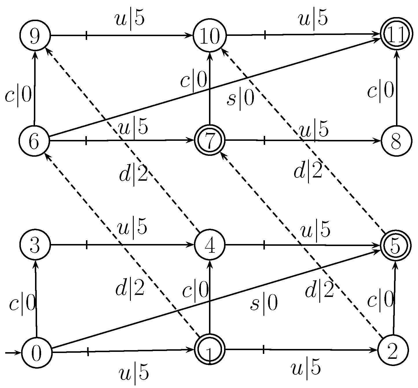
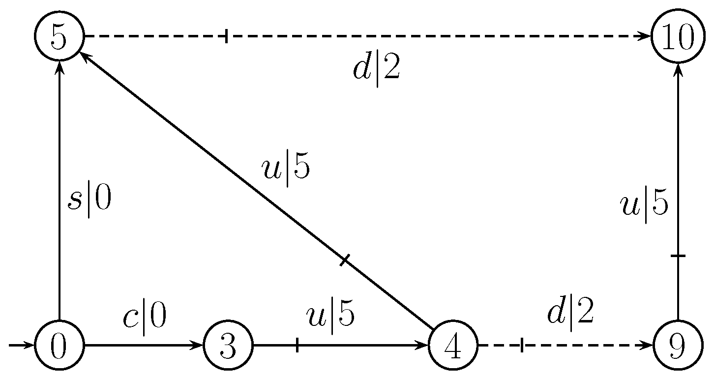
Example 5. 

We consider transition system G [1] shown in Figure 10, which models all sequences of possible moves of an agent in a three-storey building with a south wing and a north wing, both equipped with lifts and both connected by a corridor at each floor. Moreover, there is a staircase that leads from the first floor in the south wing to the third floor in the north wing. The agent starts from the first floor in the south wing. They can walk up the stairs (s) or walk through the corridors (c) from south to north without any control. The lifts can be used several times one floor upwards (u) and at most once on floor downwards (d) altogether. The moves of the lifts are controllable. Thus, ${\Sigma }_c=\{u,d\}$. The secret is that the agent is either on the second floor in the south wing or on the third floor in the north wing, i.e., $Q_s=\{1,5,7,11\}$ marked by a double circle. The adversary may gather the exact subsequence of moves in ${\Sigma }_a=\{u,c,s\}$ from sensors, but they cannot observe the downwards moves of the lifts.

For every transition of system G, the choosing cost is shown in Figure 10. In [1], there are a unique supremal prefix-closed and controllable sublanguage $L(f/G)$ (shown in Figure 11) of $L\left(G\right)$ such that secret S is opaque with respect to $L(f/G)$ and ${\Sigma }_a$. So, $V\left(\overline{K^{\prime }}\right)=V_{ϵ}\left(s\right)+V_{ϵ}\left(cuu\right)=0+0.55=0.55$.

We suppose that choosing cost $c(s,\gamma )$ is inserted in G and $g/G$, shown in Figure 10 and Figure 11, respectively. According to Line 12 of Algorithm 7 (i.e., Algorithm 3), $\underline{K^{\prime }}=\{s,cuu\}$ and $L=\{sd,cuud\}$. By the process of Algorithm 3, we have $H_1=\left\{sd\right\}$ and $H_2=\left\{cuud\right\}$, which means there exists only one path (shown in Figure 12) from the starting node to the ending node. So, $\underset{f\in {\Gamma }^{L\left(G\right)}}{min}V(L(f/G)-\overline{K^{\prime }})=V_s\left(d\right)+V_{cuu}\left(d\right)=0.2+0.002=0.202$.

At Lines 16 and 17 of Algorithm 3, it is obvious that $L(f/G)$ is shown in Figure 13, which has the minimal discount total choosing cost $V(f/G)=V(\overline{K^{\prime }},f)+V(L(f/G)-\overline{K^{\prime }})=0.55+0.202=0.752$.

The optimal supervisory control defined by $L(f/G)$ prevents the agent from using the lift of the south wing and the lift of the north wing from the second floor to the third floor at any time after they used this lift downwards, as well as the lift of the north wing downwards on the second floor.

7. Conclusions

When opacity-enforcing supervisory control is considered in Discrete Event Systems, we have to face another problem, i.e., cost. In reality, we hope we can reduce the cost while preserving the opacity of the supervised system. So, an optimal supervisory control model is formulated to enforce opacity by a supervisor with minimal discount total choosing cost. In the model, the objective function is to minimize the discount total choosing cost of closed-loop behavior, and the two constraint conditions are given: one is to enforce the opacity of closed-loop behavior, the other is to preserve the maximal part of secret information for closed-loop behavior. To solve the above optimal model, some algorithms and theorems are formulated from simplicity to complexity.

In this paper, the plant is modeled by the Finite Transition System, because coset $[·]$ and quotient set $L/[·]$ in Algorithms 3 and 4 may be infinite in Finite State Machine. To break the restriction, we will adopt a finite state to replace infinite event string and introduce the optimal control problem to Finite State Machine, which is our future work.