Displacement Reconstruction Based on Physics-Informed DeepONet Regularizing Geometric Differential Equations of Beam or Plate

Abstract

Physics-informed DeepONet (PI_DeepONet) is utilized for the reconstruction task of structural displacement based on measured strain. For beam and plate structures, the PI_DeepONet is built by regularizing the strain–displacement relation and boundary conditions, referred to as geometric differential equations (GDEs) in this paper, and the training datasets are constructed by modeling strain functions with mean-zero Gaussian random fields. For the GDEs with more than one Neumann boundary condition, an algorithm is proposed to balance the interplay between different loss terms. The algorithm updates the weight of each loss term adaptively using the back-propagated gradient statistics during the training process. The trained network essentially serves as a solution operator of GDEs, which directly maps the strain function to the displacement function. We demonstrate the application of the proposed method in the displacement reconstruction of Euler–Bernoulli beams and Kirchhoff plates, without any paired strain–displacement observations. The PI_DeepONet exhibits remarkable precision in the displacement reconstruction, with the reconstructed results achieving a close proximity, surpassing 99%, to the finite element calculations.

1. Introduction

Structural Health Monitoring (SHM) is dedicated to evaluating the health and performance of engineering structures, such as buildings, bridges, airplanes, ships, etc. Among the various parameters inspected by SHM, structural displacement is one of the most valuable pieces of information when evaluating both safety and serviceability [1,2]. By observing the long-term displacement history of a structure, the degree of deterioration and damage can be determined [3]. Given these considerations, the researchers have explored different methods to measure the displacement of structures. The methods of structural displacement measurement can be classified into two main categories: direct and indirect methods. Direct methods involve the utilization of devices such as laser displacement sensors, micrometers, radar, GPS, and digital cameras to directly capture structural displacement data [4,5]. Indirect methods generally rely on easily accessible parameters such as velocity, acceleration, and strain, which can be converted to displacement [6]. Strain is one of the most easily measurable parameters of the structure using various strain sensors, such as strain gauges and fiber Bragg grating (FBG) sensors. The FBG sensors are particularly useful for measuring strain due to their high resolution and accuracy. Moreover, the FBG strain sensors are less susceptible to environmental factors and minimally impact the structural responses. The aim of this study is to develop a method for real-time displacement reconstruction with FBG-based strain gauges.

The techniques for reconstructing displacement from surface strain measurements on a structure have been extensively studied. There are five main methods for strain-based displacement reconstruction, including the Ko method [7,8], curvature method [9,10], modal-based method [11,12], inverse finite element method (iFEM) [13,14], and deep learning method [3,15,16]. The Ko method is based on Euler–Bernoulli beam theory and reconstructs the displacement by integrating the strain segment by segment [7]. The performance of the Ko method is constrained by the assumption that the strain is linearly distributed in each segment of the beam. The curvature method reconstructs the displacement of the structure by transforming the strain information into curvature information [10], and the reconstruction accuracy is significantly influenced by the accumulated error. The modal-based method links the discrete strain with the displacement through the transformation relationship between strain and displacement mode shapes [12]. However, the modal-based method necessitates the assistance of finite element models to improve the reconstruction accuracy in most scenarios [17]. The iFEM is based on the conventional finite element method (FEM) and the weighted least-squares variational principle to reconstruct the displacement via strain [14]. This necessitates sophisticated designs of inverse finite element and measurement layout, as well as a complex programming process. In real applications, sensors cannot be applied to the entire structure due to practical constraints and economic limitations, and the insufficiently described strain field on the structure limits its implementation in accurate displacement field computations. Furthermore, the sophisticated calculations in iFEM make the real-time monitoring of structural displacement impossible [18]. In recent years, notable advancements have been achieved in the field of deep learning. Ding et al. [16] employed a back-propagation network to directly fit the relationship between strain and displacement for carbon fiber composite laminates. Moon [3] reconstructed the vertical displacement of a bridge from strains using an artificial neural network. The strain-based displacement reconstructions obtained through the deep learning method can eliminate the dependence on mechanical properties and increase computational efficiency. However, the effectiveness of the conventional deep learning method heavily relies on training datasets that include expected mechanical responses [18], and building these training datasets is often challenging and costly.

To diminish the reliance of neural networks on paired input–output observations, Raissi [19] formalized physics-informed neural networks (PINN) in 2019. In various physics and engineering scenarios, priori knowledge in the form of partial differential equations (PDEs) usually exists between input and output observations (e.g., strain–displacement equations in elastic mechanics, Navier–Stokes equations in fluid mechanics). The PINN incorporates the prior knowledge as physical loss terms into the loss function of the neural network. Guided by physical loss terms, PINN requires fewer or no paired input–output observations to be trained and provides better generalization. The application of PINN has expanded to various fields, including fluid mechanics [20], biomedicine [21], materials science [22], fracture mechanics [23], power systems [24], and scientific machine learning (SciML) [25]. Therefore, PINN is a highly promising technique for addressing the issue of displacement reconstruction.

Using PINN to reconstruct structural displacement essentially means solving a solution operator that maps the strain function to the displacement function. The Deep Operator Network (DeepONet) [26] is a novel operator learning architecture motivated by Chen’s (1995) universal approximation theorem [27]. The DeepONet significantly reduces the computational cost of solving operator regression problems and provides better generalization and faster convergence compared to traditional fully connected networks. Drawing inspiration from PINN, physics-informed DeepONet (PI_DeepONet) [28] was proposed to efficiently learn a solution operator of PDEs. The PI_DeepONet is an extension of DeepONet and satisfies the underlying PDEs by incorporating them into the loss function of the DeepONet. The PI_DeepONet has shown good performance in diverse fields, such as the prediction of crack path [29], solving heat conduction equations [30], and the prediction of instability waves in hypersonic boundary layers [31].

In this paper, PI_DeepONet is applied to solve geometric differential equations (GDEs) of beam and plate structures with various restrictions. According to the Euler–Bernoulli beam theory and the Kirchhoff plate theory, the strain–displacement relations and boundary conditions of a structure are represented in the differential form. The strain–displacement relations, together with the boundary conditions of the structure, are called GDEs in this paper. Utilizing the automatic differentiation techniques in deep learning [32,33], each GDEs equation is formulated as a loss term of the PI_DeepONet. The PI_DeepONet used to regularize the GDEs is trained to be a solution operator of GDEs, and the solution operator of the beam or plate is utilized to directly map the strain function to the displacement function under diverse loading conditions. Compared to traditional methods, such as the finite difference method (FDM) [34] and the finite element method (FEM), PI_DeepONet is a mesh-free approach and could break the curse of dimensionality [33].

Due to the insufficient understanding of the regular mechanism at present, PINN has a tendency to converge to an incorrect solution in some scenarios. The loss function of PINN is a weighted combination of different loss terms, resulting in low training efficiency if the weights are selected inappropriately. Therefore, many methods have been proposed to assign a proper weight to each loss term. Bu et al. [35] proposed two approaches, named annealing and cold start, to tune the weights of the loss terms in the initial or final period. Remco et al. [36] obtained optimal weights by defining the upper and lower bounds for different loss terms. However, these non-adaptive methods cannot guarantee that the assigned weights remain optimal throughout the entire PINN training process. Research has been implemented to adaptively balance the interplay among loss terms. Kim et al. [37] utilized the Dynamic Pull Method (DPM) to dynamically manipulate the weights of each loss term during the training process of PINN. Xiang et al. [38] built Gaussian probabilistic models for loss terms and adaptively updated the learning weights based on maximum likelihood estimation. These methods are dedicated to balancing the interplay between loss terms via the magnitudes of the loss terms, but pay little attention to the backpropagation gradients of each loss term with respect to the parameters of PINN. However, the gradients are essential for updating the parameters through the gradient descent method. Wang [39] highlighted that the gradients of each loss term may become extremely unbalanced during the training process. In that scenario, the neural network may struggle to fit each loss term evenly, resulting in incorrect convergence. To maintain the balance in the gradients of loss terms of the PI_DeepONet during the training process, we propose an algorithm that can update the weights adaptively, utilizing the back-propagated gradient statistics.

In this paper, the PI_DeepONet is constructed to serve as the solution operator of GDEs in beam and plate structures, which can efficiently solve the GDEs to reconstruct the displacement from strain under various loading conditions. This paper is structured as follows. In Section 2, the GDEs of the beam and plate under various restrictions are constructed. In Section 3, we provide the framework and implement the PI_DeepONet for the displacement reconstruction of beam and plate structures. The algorithm used to update weights adaptively according to the gradient statistics of each individual loss is also proposed in Section 3. In Section 4, the effectiveness of PI_DeepONet in the application of displacement reconstruction is validated via FEM. In Section 5, we present the main conclusions of our research.

2. Problem Description

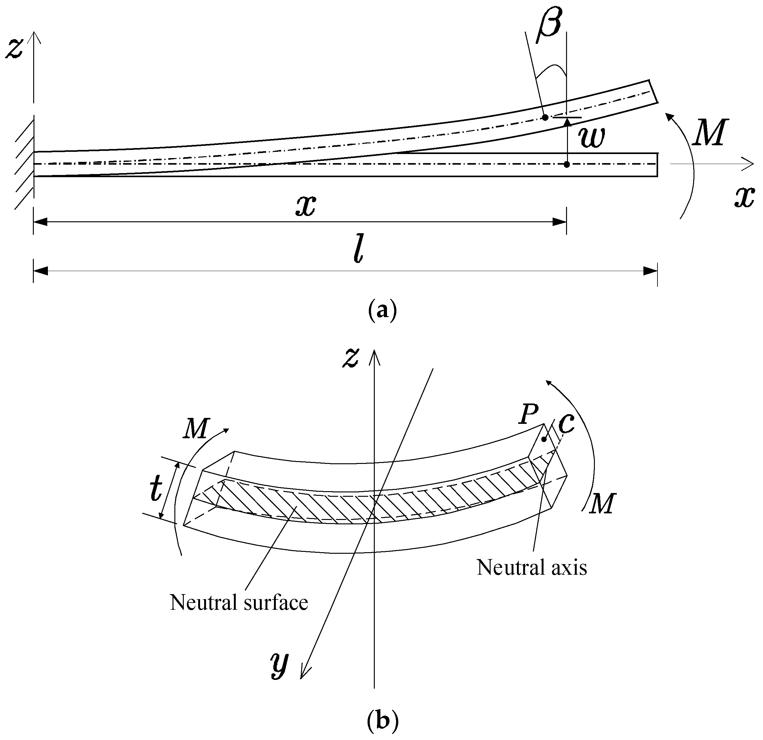
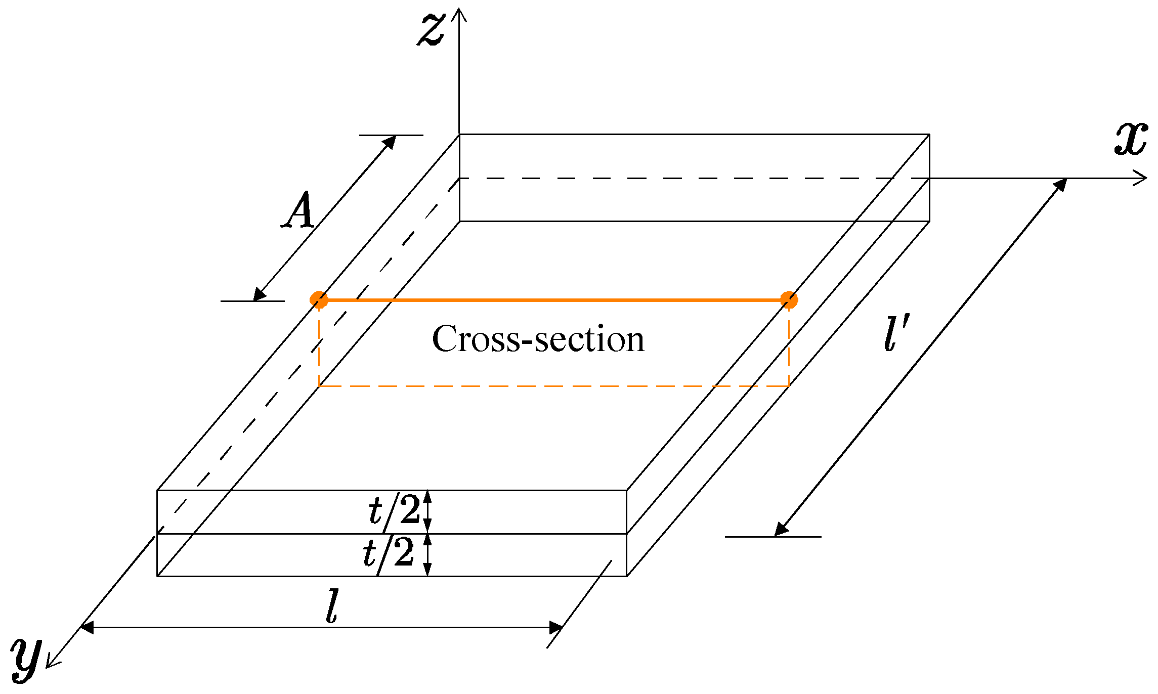
This paper focuses on reconstructing the displacement of Euler–Bernoulli beams and Kirchhoff plates. Figure 1 illustrates the Cartesian coordinate system used for the beam analysis in this study.

Figure 1. Cartesian coordinate system used for the beam analysis: (a) displacement of the beam and (b) micro-segment of the beam.

In Figure 1, the $x$ -coordinate is taken along the length of the beam; the $z$ -coordinate is taken along the thickness (the height) of the beam. The $\beta$ denotes the rotating angle of the cross-section and $w$ denotes the vertical displacement along the coordinate $z$. The beam has a length of $l$ and a thickness of $t$. According to Euler–Bernoulli beam theory (EBT), the normal strain at point $P$ on the cross-section of the beam can be expressed as follows:

$${\epsilon }_x^P=\frac{-c}{\rho }$$

(1)

in which $c$ is the perpendicular distance from the point $P$ to the neutral axis and $\rho$ is the radius of curvature of the neutral surface of the beam. In the case of small displacements, the curvature of the neutral surface can be expressed as follows:

$$\frac{1}{\rho }=\pm \frac{w^{″}}{{\left(1+{w^{\prime }}^2\right)}^{3/2}}\approx \pm w^{″}=\frac{d^{2}w}{d{x}^2}$$

(2)

By aligning Equation (2) with Equation (1), the relationship between strain and displacement at point $P$ can be expressed as follows:

$${\epsilon }_x^P=-c\frac{d^{2}w\left(x_P\right)}{d{x}^2}$$

(3)

in which $x_P$ is the coordinate of point $P$ along the coordinate $x$. In practice, strain measuring points can only be arranged at the surface of the beam. For beams with regular cross-sections and uniform thickness, the distance, $c$, from the strain measuring points to the neutral axis is half of the thickness, $t$. Therefore, based on Equation (3), the strain–displacement relation on the upper surface of the beam can be expressed as follows:

$${\epsilon }_x\left(x\right)=-0.5t\frac{d^{2}w\left(x\right)}{d{x}^2},\hspace{1em}x\in \left[0,l\right]$$

(4)

Figure 2 illustrates the Cartesian coordinate system used for the plate analysis, in which $t$ denotes the thickness and $(l,l^{\prime })$ denotes the lengths along the coordinate axes, respectively.

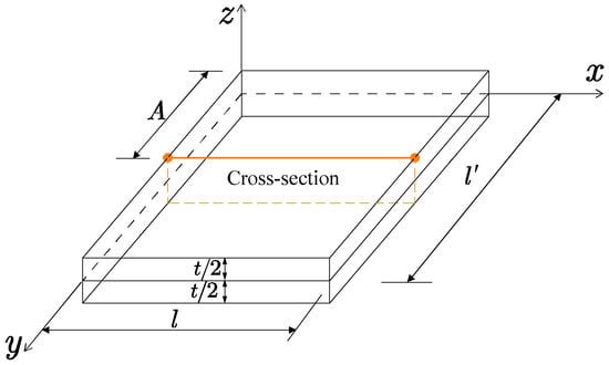
Figure 2. Cartesian coordinate system used for the plate analysis.

According to the classical Kirchhoff plate theory (CPT), the shear strains ${\gamma }_{zx}$ and ${\gamma }_{zy}$ of the plate remain zero, which can be written as follows:

$$\{\begin{array}{l}{\gamma }_{zx}=\frac{\partial u}{\partial z}+\frac{\partial w}{\partial x}=0\hfill \\ {\gamma }_{zy}=\frac{\partial v}{\partial z}+\frac{\partial w}{\partial y}=0\hfill \end{array}$$

(5)

where $\left(u,v\right)$ are the displacement components along the $\left(x,y\right)$ coordinate directions, respectively, and $w$ is the vertical displacement along coordinate $z$. Integrating Equation (5) while taking into account that ${\left(u\right)}_{z=0}=0$ and ${\left(v\right)}_{z=0}=0$ in CPT, the geometric relationship between $u$, $v$ and $w$ can be obtained as follows:

$$\{\begin{array}{l}u=-z\frac{\partial w}{\partial x}\hfill \\ v=-z\frac{\partial w}{\partial y}\hfill \end{array}$$

(6)

Considering that the strain measuring points can only be located on the surface of the plate in practice, we take the first derivative on both sides of Equation (6). Therefore, the strain–displacement relation on the surface of the plate can be expressed as follows:

$$\{\begin{array}{l}{\epsilon }_x\left(x,y\right)=-0.5t\frac{{\partial }^{2}w\left(x,y\right)}{\partial x^2}\hfill \\ {\epsilon }_y\left(x,y\right)=-0.5t\frac{{\partial }^{2}w\left(x,y\right)}{\partial y^2}\hfill \end{array},\hspace{1em}\left(x,y\right)\in \left[0,l\right]\times [0,l^{\prime }]$$

(7)

in which (${\epsilon }_x$,${\epsilon }_y$ ) are the strain components along the $\left(x,y\right)$ coordinate directions, respectively. For the line (see Figure 2) at $y=A(A\in [0,l^{\prime }\left]\right)$ on a cross-section parallel to the plane $xOz$, the strain–displacement relation (7) of the plate degenerates into the same form as that of the beam. Therefore, we only need the strain along the $x$ coordinate direction to reconstruct the vertical displacement of the cross-section at $y=A$.

The boundary restrictions of the beam or plate are categorized as free, simply supported, clamped, and elastically supported. We neglect the case of elastically supported boundary restrictions and consider only the geometric boundary conditions specifying $w$ or $\frac{dw}{dx}$. The corresponding boundary conditions for each restriction are presented in Table 1.

Table 1. Boundary conditions for different restrictions.

Restriction	Boundary Conditions
Free	$w$ or $\frac{dw}{dx}$ are not specified
Simply supported	$w=0$
Clamped	$w=0,\frac{dw}{dx}=0$

The strain–displacement relations, together with the boundary conditions of the structure, are referred to as GDEs in this paper. In Table 1, the boundary conditions can be categorized into the Dirichlet boundary condition, specifying $w$, and the Neumann boundary condition, specifying $\frac{dw}{dx}$. To facilitate the training of the network, the Dirichlet boundary conditions at all boundaries are combined into one equation. As such, the general form of the GDEs can be expressed as follows:

$$\{\begin{array}{l}\mathcal{P}\left(x,\epsilon ,w\right)=0,\hspace{1em}\hspace{1em}x\in \Omega \hfill \\ {\mathcal{N}}_i\left(x,\epsilon ,w\right)=0,\hspace{1em}\hspace{1em}x\in \partial {\Omega }_i,i=1,\dots ,H\hfill \\ \mathcal{D}\left(x,\epsilon ,w\right)=0,\hspace{1em}\hspace{1em}x\in \partial {\Omega }_1+\partial {\Omega }_2+\dots +\partial {\Omega }_J\hfill \end{array}$$

(8)

in which $\mathcal{P}$ is the general differential operator that defines the strain–displacement relation, ${\left\{{\mathcal{N}}_i\right\}}_{i=1}^H$ and $\mathcal{D}$ denote the Neumann boundary conditions and Dirichlet boundary conditions, respectively, $H$ and $J$ denote the numbers of Neumann boundary conditions and Dirichlet boundary conditions, respectively, and $\Omega \subset ℝ$ and $\partial \Omega$ denote the geometric domain and the boundary region of the structure, respectively.

In summary, solving the GDEs under different loading conditions with the full-field strain, as described in Equation (8), can reconstruct the structural displacement. However, the arrangement of strain measuring points is constrained in practice, resulting in an unknown strain distribution between adjacent measuring points. Therefore, the numerical solution of GDEs is confronted with inherent challenges. Indeed, the process of reconstructing displacement from strain under different loading conditions essentially constitutes an operator regression problem. To effectively perform the operator regression while removing the dependence on full-field strain, a physics-informed DeepONet based on the GDEs is constructed in this paper.

3. Methodology

3.1. Physics-Informed DeepONet

DeepONet was designed to acquire abstract nonlinear operator mapping functions between Banach spaces of infinite dimensions [26]. Compared to fully connected neural networks, DeepONet significantly decreases the generalization error while guaranteeing a smaller approximation error. By introducing an efficient regular mechanism, PI_DeepONet biases the output of the DeepONet model to ensure physical consistency. Here, we present a brief overview of the concept and architecture of the PI_DeepONet.

Let $\mathcal{U}$ and $\mathcal{W}$ be two separate branch spaces. Our purpose is to learn the solution operator $G$ that maps strain function $\epsilon \in \mathcal{U}$ to displacement function $w\in \mathcal{W}$, which is defined as follows:

$$G\left(\epsilon \right)=w$$

(9)

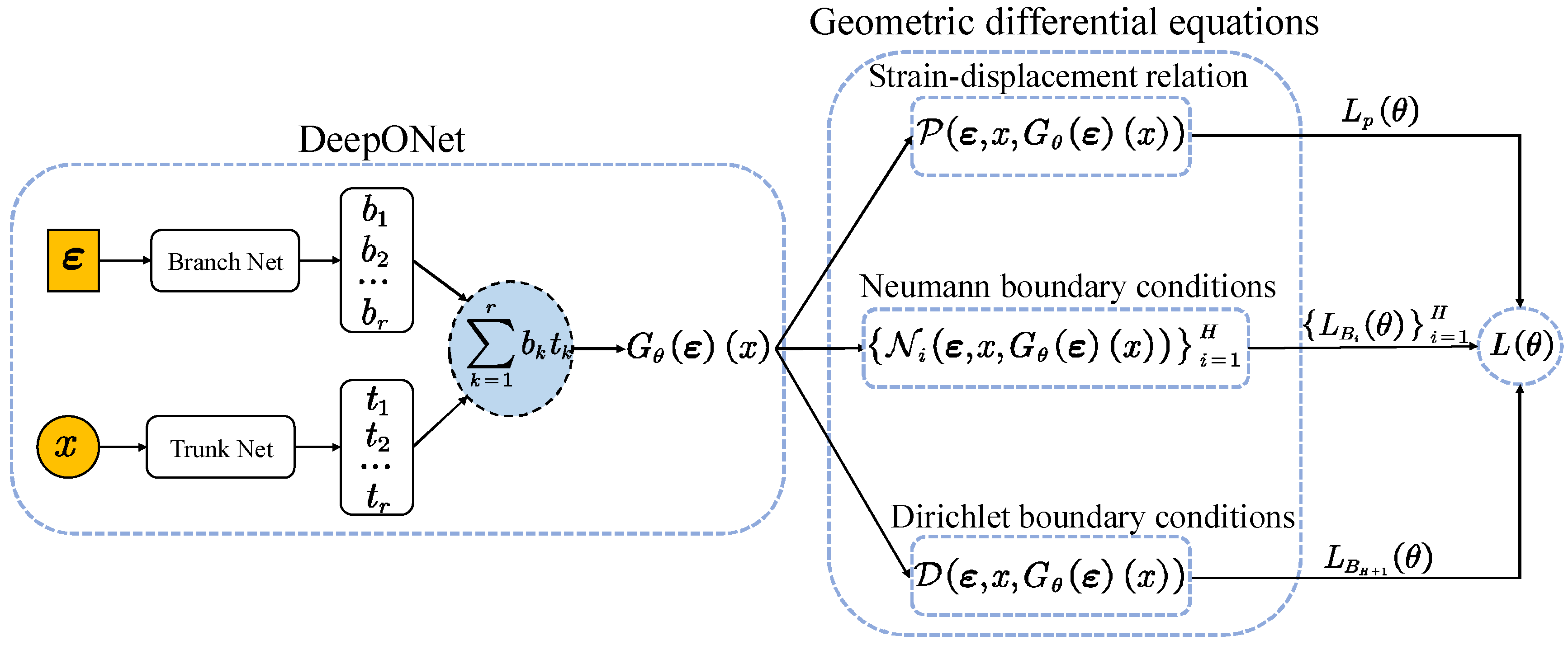
The solution operator $G$ is represented by the DeepONet $G_{\theta }$, in which $\theta$ denotes all trainable parameters of the DeepONet. The architecture of the DeepONet is shown in Figure 3. The DeepONet consists of two separate neural networks, called branch net and trunk net, respectively.

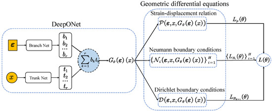
Figure 3. Architecture of physics-informed DeepONet regularizing geometric differential equations.

The branch net receives the strain function $\epsilon$ as its input. The strain values at $m$ locations are used for the expression of the strain function $\epsilon$ as follows:

$$\epsilon =[\epsilon {(x}^{\left(1\right)}),\epsilon {(x}^{\left(2\right)}),\cdots ,\epsilon {(x}^{\left(m\right)})]$$

(10)

After the $\epsilon$ is fed into the branch net, a feature embedding ${\left[b_1,b_2,\dots ,b_{\begin{array}{c}r\end{array}}\right]}^T\in {ℝ}^r$ is returned as the output. The trunk net receives the coordinate $x$ as an input, which is one-dimensional in this paper. The feature embedding ${\left[t_1,t_2,\dots ,t_{\begin{array}{c}r\end{array}}\right]}^T\in {ℝ}^r$ is the output of the trunk network. It is worth noting that the output layers of both the trunk net and the branch net consist of the same number of neurons. The number of neurons in the input layer of the trunk net and branch net can be determined based on the dimension of the inputs $x,\epsilon$. The final output of DeepONet is obtained by computing the inner product of the feature embeddings of the trunk net and branch net. Thus, after inputting the strain function $\epsilon$ and the coordinate $x$, DeepONet returns the displacement prediction at the $x$ coordinate as follows:

$$G_{\theta }\left(\epsilon \right)\left(x\right)={\displaystyle \sum _k^r{b}_k\left(\epsilon \left(x^{\left(1\right)}),\epsilon \right(x^{\left(2\right)}),\cdots ,\epsilon \left(x^{\left(m\right)}\right)\right)t_k\left(x\right)}={\displaystyle \sum _{k=1}^r{b}_k{t}_k}$$

(11)

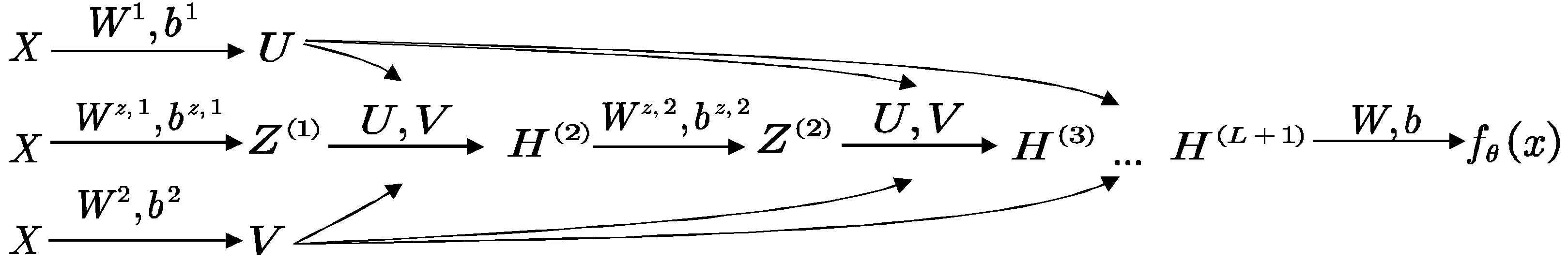
Classical networks, such as the fully connected neural network (FNN), convolutional neural network (CNN), or recurrent neural network (RNN), can be chosen as the trunk net and brank net according to the input structure. In this paper, an improved fully connected network architecture, proposed by Wang et al. [39], is employed. In contrast to the FNN, the improved architecture introduces two transformer networks that map the input variables to a high-dimensional feature space. The improved architecture explicitly considers multiplicative interactions among input dimensions and enhances the hidden states by introducing residual connections. The forward-propagation of the improved architecture can be expressed as follows:

$$U=\sigma \left(X{W}^1+b^1\right),V=\sigma \left(X{W}^2+b^2\right)$$

(12)

$$Z^{\left(1\right)}=\sigma \left(X{W}^{z,1}+b^{z,1}\right)$$

(13)

$$H^{(k+1)}=\left(1-Z^{\left(k\right)}\right)\odot U+Z^{\left(k\right)}\odot V,\hspace{1em}k=1,\dots ,L$$

(14)

$$Z^{\left(k\right)}=\sigma \left(H^{\left(k\right)}{W}^{z,k}+b^{z,k}\right),\hspace{1em}k=2,\dots ,L$$

(15)

$$f_{\theta }\left(x\right)=H^{(L+1)}W+b$$

(16)

In Equations (12)–(16), $\odot$ represents the inner product matrix multiplication, $\sigma$ represents the activation function, $X$ represents the input to the network, $W$ and $b$ represent the weights and bias of each layer of the network, and $f_{\theta }\left(x\right)$ represents the final output of the network. The new network requires additional training of the weights and biases of the two transformer networks compared to the FNN. Figure 4 illustrates the architecture of the new network.

Figure 4. Architecture of the new network serving as the trunk net and branch net.

The training dataset of the DeepONet is a triplet $\left[\epsilon ,x,w\left(x\right)\right]$ which takes the following form:

$$\left[\left[\begin{array}{c}⋮\\ {\mathbf{\epsilon }}_i \left(x^{\left(1\right)}\right),{\mathbf{\epsilon }}_i \left(x^{\left(2\right)}\right),\cdots ,{\mathbf{\epsilon }}_i \left(x^{\left(m\right)}\right)\\ {\mathbf{\epsilon }}_i \left(x^{\left(1\right)}\right),{\mathbf{\epsilon }}_i \left(x^{\left(2\right)}\right),\cdots ,{\mathbf{\epsilon }}_i \left(x^{\left(m\right)}\right)\\ ⋮\\ {\mathbf{\epsilon }}_i \left(x^{\left(1\right)}\right),{\mathbf{\epsilon }}_i \left(x^{\left(2\right)}\right),\cdots ,{\mathbf{\epsilon }}_i \left(x^{\left(m\right)}\right)\\ ⋮\end{array}\right],\left[\begin{array}{c}⋮\\ x^{\left(1\right)}\\ x^{\left(2\right)}\\ ⋮\\ x^{\left(P\right)}\\ ⋮\end{array}\right],\left[\begin{array}{c}⋮\\ {\mathbf{\omega }}_i \left(x_1\right)\\ {\mathbf{\omega }}_i \left(x_2\right)\\ ⋮\\ {\mathbf{\omega }}_i \left(x_P\right)\\ ⋮\end{array}\right]\right]$$

(17)

in which ${\left\{{\epsilon }_i\right\}}_{i=1}^N$ denote $N$ separate strain functions, ${\left\{x_j\right\}}_{j=1}^P$ denote $P$ coordinates in the domain of $G_{\theta }\left({\epsilon }_i\right)$, and $w_i\left(x_j\right)$ is the corresponding true displacement observed at $x_{\begin{array}{c}j\end{array}}$. The loss of the DeepONet during training in the form of mean square error can be expressed as follows:

$$L_d\left(\theta \right)=\frac{1}{NP}{\displaystyle \sum _{i=1}^N{\displaystyle \sum _{j=1}^P{\left|G_{\theta }\left({\epsilon }_i\right)\left(x_j\right)-w_i\left(x_j\right)\right|}^2}}$$

(18)

where $L_d\left(\theta \right)$ is the loss determined by paired strain–displacement observations, called data-driven loss.

As a purely data-driven network, the prediction error and generalization error of the DeepONet heavily depend on the quantity and quality of the training data. To eliminate the necessity for training data, GDEs can be formulated as the loss terms of the DeepONet used to construct the PI_DeepONet, as shown in Figure 3.

To construct the PI_DeepONet, let $\epsilon ,x$ be the inputs of the branch net and trunk net of the DeepONet, respectively, and $G_{\theta }\left(\epsilon \right)\left(x\right)$ be the output of the DeepONet; then, the physical constraint residuals generated by the lack of satisfaction of the GDEs can be expressed as follows:

$$R_p\left(\theta \right)\left(x,\epsilon \right)=\left|\left(x,\epsilon \left(x\right),G_{\theta }\left(\epsilon \right)\left(x\right)\right)\right|$$

(19)

$$R_{N_i}\left(\theta \right)\left(x,\epsilon \right)=\left|{\mathcal{N}}_i\left(x,\epsilon \left(x\right),G_{\theta }\left(\epsilon \right)\left(x\right)\right)\right|,\hspace{1em}i=1,\dots ,H$$

(20)

$$R_D\left(\theta \right)\left(x,\epsilon \right)=\left|\mathcal{D}\left(x,\epsilon \left(x\right),G_{\theta }\left(\epsilon \right)\left(x\right)\right)\right|$$

(21)

in which $R_p$, $R_{N_i}$, and $R_D$ are the residuals generated by the unsatisfaction of the strain–displacement relation, Neumann boundary conditions, and Dirichlet boundary conditions defined in GDEs, respectively. Then, the loss function, in the form of the mean square error computed by physical constraint residuals, can be expressed as follows:

$$L_p\left(\theta \right)=\frac{1}{Nm}{\displaystyle \sum _{i=1}^N{\displaystyle \sum _{j=1}^m{\left|R_p\left(\theta \right)\left(x^{\left(j\right)},{\epsilon }_i\right)\right|}^2}}$$

(22)

$$L_{B_i}\left(\theta \right)=\frac{1}{N{Q}_i}{\displaystyle \sum _{k=1}^N{\displaystyle \sum _{j=1}^{Q_i}{\left|R_{N_i}\left(\theta \right)\left(x_{B_i}^{\left(j\right)},{\epsilon }_{\begin{array}{c}k\end{array}}\right)\right|}^2},\hspace{1em}i=1,\dots ,H}$$

(23)

$$L_{B_{H+1}}\left(\theta \right)=\frac{1}{N{Q}_{H+1}}{\displaystyle \sum _{k=1}^N{\displaystyle \sum _{j=1}^{Q_{H+1}}{\left|R_D\left(\theta \right)\left(x_{B_{H+1}}^{\left(j\right)},{\epsilon }_{\begin{array}{c}k\end{array}}\right)\right|}^2}}$$

(24)

in which $L_p\left(\theta \right)$ and ${\left\{L_{B_i}\left(\theta \right)\right\}}_{i=1}^{H+1}$ are the losses of the strain–displacement relation and boundary conditions, ${\left\{x^{\left(j\right)}\right\}}_{j=1}^m$ are $m$ locations at which the strain is used for the expression of the strain function $\epsilon$, and ${\left\{x_B^{\left(j\right)}\right\}}_{j=1}^{Q_i}$ are sets of collocation points sampled from the corresponding boundary region. The $L_p\left(\theta \right)$ and ${\left\{L_{B_i}\left(\theta \right)\right\}}_{i=1}^{H+1}$ are computed in the complete absence of paired strain–displacement observations, called physics-driven losses. By adding physics-driven losses to the data-driven loss of the DeepONet, PI_DeepONet is constructed. In fact, the solution operator mapping the strain function into the displacement function can be completely defined by the GDEs. Thus, the PI_DeepONet can converge to the correct solution operator by minimizing only the physics-driven losses. As such, the aggregate loss of the PI_DeepONet we constructed can be expressed as follows:

$$L\left(\theta \right)={\lambda }_p{L}_p\left(\theta \right)+{\displaystyle \sum _{i=1}^{H+1}{\lambda }_i{L}_{B_i}\left(\theta \right)}$$

(25)

in which ${\lambda }_p$ and ${\lambda }_i$ are the weights used to equalize the losses. The weights of the losses can be chosen empirically or adjusted as hyperparameters of the network.

3.2. Implementation of the PI_DeepONet

In this section, we provide a concise overview of the implementation of the PI_DeepONet described above. The building and training process of all the PI_DeepONet described in this paper are implemented in the JAX framework.

To reconstruct the displacement in different scenarios, it is imperative to build a PI_DeepONet with an appropriate architecture. The architecture of the PI_DeepONet needs to be determined based on the arrangement of the strain measuring points. To predict the displacement $w$ via strain $\epsilon$, let the coordinates of surface strain measuring points be ${\left\{x^{\left(i\right)}\right\}}_{i=1}^m$. The numbers of neurons in the input layer of the branch net and the trunk net are equal to the dimensions of coordinate $x^{\left(i\right)}$ and the measured strain $\epsilon$, respectively. There is no specific requirement for the hidden layer architectures of the trunk net and branch net, but they can be adjusted appropriately to improve the fitting ability of the PI_DeepONet. All the trunk nets and branch nets of the PI_DeepONet built in this paper have three hidden layers, with 1000 neurons per layer. After the architecture of the PI_DeepONet is determined, the physics-driven losses are determined based on the GDEs of the structure.

Training the PI_DeepONet necessitates the construction of a training dataset for each physics-driven loss. The trained PI_DeepONet serving as the solution operator should be capable of providing the solution function of the GDEs for arbitrary function inputs. Therefore, function $\epsilon$, used for training the PI_DeepONet, is not required to be derived from simulation or experimentation. Here, we used mean-zero Gaussian random fields (GRF) to model random strain functions ${\epsilon }^r$ to construct the corresponding training datasets for each physics-driven loss as follows:

$${\epsilon }^r~\mathcal{G}\left(0,k_l\left(x_1,x_2\right)\right)$$

(26)

with an exponential quadratic covariance kernel $k_l(x_1,x_2)=\exp (-||x_1-x_2|{|}^2/2l^2)$ with a length scale parameter $l$ > 0. The parameter $l$ determines the complexity of the ${\epsilon }^r$, and a larger $l$ will produce a smoother ${\epsilon }^r$. The ${\epsilon }^r$ are represented by discrete values evaluated at the coordinates of the strain measuring points of the structure. We only need quantities of strain, instead of paired strain–displacement observations, to construct the training datasets. Different physics-driven losses correspond to the different training datasets. For instance, the training dataset of $L_p\left(\theta \right)$ takes the following form:

$$\left[\left[\begin{array}{c}⋮\\ {\mathit{\epsilon }}_i^r\left(x^{\left(1\right)}\right),{\mathit{\epsilon }}_i^r\left(x^{\left(2\right)}\right),\cdots ,{\mathit{\epsilon }}_i^r\left(x^{\left(m\right)}\right)\\ {\mathit{\epsilon }}_i^r\left(x^{\left(1\right)}\right),{\mathit{\epsilon }}_i^r\left(x^{\left(2\right)}\right),\cdots ,{\mathit{\epsilon }}_i^r\left(x^{\left(m\right)}\right)\\ ⋮\\ {\mathit{\epsilon }}_i^r\left(x^{\left(1\right)}\right),{\mathit{\epsilon }}_i^r\left(x^{\left(2\right)}\right),\cdots ,{\mathit{\epsilon }}_i^r\left(x^{\left(m\right)}\right)\\ ⋮\end{array}\right],\left[\begin{array}{c}⋮\\ x^{\left(1\right)}\\ x^{\left(2\right)}\\ ⋮\\ x^{\left(m\right)}\\ ⋮\end{array}\right],\left[\begin{array}{c}⋮\\ {\mathit{\epsilon }}_i^r\left(x^{\left(1\right)}\right)\\ {\mathit{\epsilon }}_i^r\left(x^{\left(2\right)}\right)\\ ⋮\\ {\mathit{\epsilon }}_i^r\left(x^{\left(m\right)}\right)\\ ⋮\end{array}\right]\right]$$

(27)

in which ${\left\{{\epsilon }_i^r\right\}}_{i=1}^N$ denotes $N$ separate random strain functions, modeled by GRF.

The PI_DeepONet can be trained once the training datasets have been constructed. The PI_DeepONet is first initialized using the Glorot normal scheme and then updates the parameters using a small-batch stochastic gradient descent method [28], expressed as follows:

$${\theta }_{n+1}={\theta }_n-\frac{\eta }{\Phi }\sum _{k=1}^{\Phi }({\lambda }_p{\nabla }_{\theta }{L}_p^k\left({\theta }_n,x_k,{\epsilon }_k\right)+\sum _{i=1}^{H+1}{\lambda }_i{\nabla }_{\theta }{L}_{B_i}^k\left({\theta }_n,x_k,{\epsilon }_k\right))$$

(28)

in which $L_p^k\left({\theta }_n\right)={\left|R_p\left({\theta }_n\right)\left(x_k,{\epsilon }_k\right)\right|}^2$, $L_{B_i}^k\left({\theta }_n\right)={\left|R_{B_i}\left({\theta }_n\right)\left(x_k,{\epsilon }_k\right)\right|}^2$, $\Phi$ denotes the batch size in the training process and $\eta$ denotes the learning rate. The $\Phi$ is set to be 256 in this paper. In the training process of the PI_DeepONet, physics-driven losses are computed using their corresponding training datasets; then, the aggregate loss $L\left(\theta \right)$ is computed by a weighted sum of the losses. The $L\left(\theta \right)$ is minimized using the Adam optimizer with an initial learning rate of 0.001. We used exponential learning rate decay with a decay rate of 0.9 every 1000 training iterations. The hyperbolic tangent function (Tanh) was used as the activation function for the PI_DeepONet. We minimized the loss of PI_DeepONet for 80,000 iterations and recorded the state of the PI_DeepONet every 100 iterations.

3.3. Updating Weights Adaptively for the PI_DeepONet

In contrast to the Dirichlet boundary condition, the Neumann boundary condition is formed with partial derivative terms. Thus, the loss terms of the PI_DeepONet will become fairly complex for GDEs with multiple Neumann boundary conditions. Due to the insufficient understanding of the regular mechanism at present, PI_DeepONet has a tendency to converge to an incorrect solution when the loss terms of the PI_DeepONet are complex.

Using gradient descent to update the parameters of the PI_DeepONet, the $n$ -th step of gradient descent can be expressed as Equation (28). The gradients used to update the parameters are a weighted sum of the gradients of each individual loss. Thus, in situations where the gradients of each individual loss exhibit significant imbalance, the gradients with smaller values are more likely to be underestimated, resulting in poor fitting for the corresponding physics-driven loss. The imbalance of the gradients of each individual loss is quite serious when the PI_DeepONet has complex loss terms. As such, it is essential to employ effective measures to alleviate the imbalance among the gradients of each loss.

In fact, the imbalance can be mitigated by selecting appropriate weights for each loss. However, the gradient distributions of the losses change constantly throughout the training process. Therefore, it is not feasible to establish a predetermined set of weights to maintain balanced gradient distributions during the whole training process. To address that issue, an algorithm for updating weights adaptively is proposed, as summarized in Algorithm 1. Algorithm 1 is designed to automatically adjust the weights during model training using the back-propagated gradient statistics. The gradient distributions of each loss will remain balanced after the updated weights are applied.

Algorithm 1: Updating weights adaptively for the PI_DeepONet
Consider a PI_DeepONet $G_{\theta }\left(u\right)\left(x\right)$ with parameters $\theta$ and a loss function
$$L\left(\theta \right)={\lambda }_s{L}_s\left(\theta \right)+{\displaystyle \sum _{i=1}^M{\lambda }_i{L}_i\left(\theta \right)}$$ (29)
in which $L_s\left(\theta \right)$ is the base loss for the updating of weights; ${\left\{L_i\left(\theta \right)\right\}}_{i=1}^M$ represents all other losses; $\lambda$ represents the weight of each loss. Then, use $S$ steps of a gradient descent algorithm to update the parameters $\theta$ as follows: for $n=1,\cdots ,S$ do
	(a) Calculate the transit weights ${\widehat{\lambda }}_i$ as follows: $${\widehat{\lambda }}_i={\lambda }_s\frac{\overline{\left|{\nabla }_{{\theta }^t}{L}_s\left({\theta }_n\right)\right|}+\overline{\left|{\nabla }_{{\theta }^b}{L}_s\left({\theta }_n\right)\right|}}{\overline{\left|{\nabla }_{{\theta }^t}{L}_i\left({\theta }_n\right)\right|}+\overline{\left|{\nabla }_{{\theta }^b}{L}_i\left({\theta }_n\right)\right|}},\hspace{1em}i=1,2,\dots ,M$$ (30)
	in which $\overline{\left|{\nabla }_{\theta }L\left({\theta }_n\right)\right|}$ denotes the average of the absolute values of the gradients of $L\left({\theta }_n\right)$ with respect to parameters $\theta$, ${\theta }^{\begin{array}{c}t\end{array}}$ denotes all parameters of the trunk net, and ${\theta }^b$ denotes all parameters of the branch net. (b) Update the weights ${\lambda }_i$ using a weighted average of the following form: $${\lambda }_i=\left(1-\alpha \right){\lambda }_i+\alpha {\widehat{\lambda }}_i,\hspace{1em}i=1,2,\dots ,M$$ (31)
	(c) Update the parameters $\theta$ using the following gradient descent: $${\theta }_{n+1}={\theta }_n-\eta {\lambda }_s{\nabla }_{\theta }{L}_s\left({\theta }_n\right)-\eta {\displaystyle \sum _{i=1}^M{\lambda }_i{\nabla }_{\theta }{L}_i\left({\theta }_n\right)}$$ (32)
end
Hyper-parameter $\alpha$ is recommended to be 0.9.

Due to the stochasticity of the gradient descent updates, it is expected that the instantaneous values of the gradients computed above will exhibit high variance. Thus, the hyper-parameter $\alpha$ is introduced to Algorithm 1, and the actual weights ${\lambda }_i$ are weighted averages based on their previously calculated values. The updates of the weights in Equations (30) and (31) can occur at every iteration of the gradient descent loop or at a user-specified frequency (e.g., every 100 gradient descent steps). When Algorithm 1 is utilized for the network training in this paper, weights assigned the initial value of 1 are updated at a frequency of one iteration, and the loss of Dirichlet boundary condition is selected as the base loss.

4. Results

In this section, we validate the effectiveness of PI_DeepONet in displacement reconstruction. The strain and displacement of the structure under various loading conditions were simulated by FEM. Using the simulated strains in the selected strain measurement points and the coordinates of displacement measurement points as the inputs, the PI_DeepONet output the reconstructed displacements. The performance of PI_DeepONet was evaluated by comparing the reconstructed displacement with the FEM calculation.

The finite element method calculates displacements by solving the global stiffness equation under known loading conditions and boundary conditions. The global stiffness equation of a structure is expressed as follows:

$$Kd=R$$

(33)

in which $K$ denotes the global stiffness matrix; $d$ and $R$ denote the global node displacement and global node force. After the $d$ is solved, the strain ${\epsilon }^e$ in each element can be calculated as follows:

$${\epsilon }^e=B{d}^e$$

(34)

in which $B$ denotes the element strain matrix and $d^e$ denotes the element node displacement.

4.1. Beam

Here, we evaluate the reconstruction performance of PI_DeepONet for rectangular section beams with various restrictions. The beams with an elastic modulus of 210 Gpa and a Poisson’s ratio of 0.3 were simulated by the finite element analysis software ANSYS2021R1.

4.1.1. Displacement Reconstruction for Rectangular Section Beam

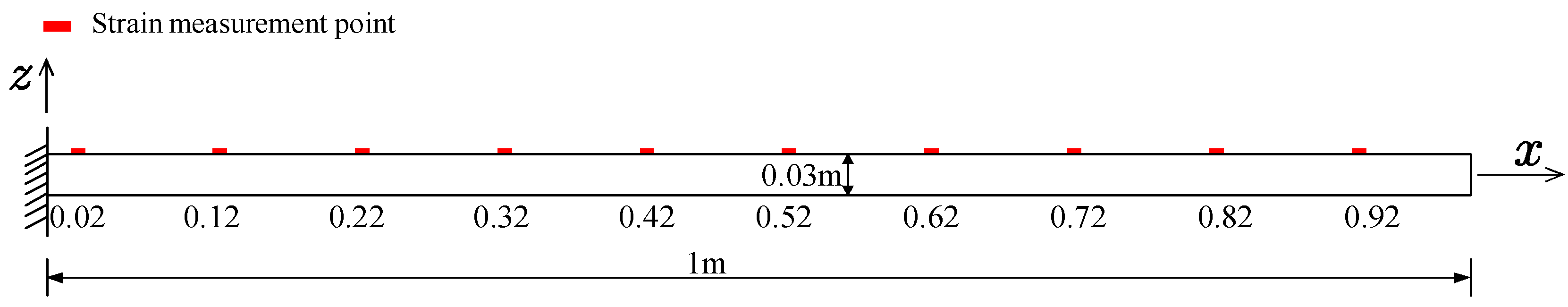
This section focuses on reconstructing the displacement for the rectangular section beam with different restrictions. The restrictions of the beam used for the displacement reconstruction were clamped at one end, simply supported–simply supported, clamped–simply supported, and clamped–clamped. Figure 5 shows the geometric model of the beam with one end clamped. The thickness of the beam is 0.03 m. To reconstruct the vertical displacement, 10 strain measuring points were arranged on the surface of the beam, as shown in Figure 5. The $x$ coordinates of the strain measuring points are ${\left\{0.02+0.1\left(i-1\right)\right\}}_{i=1}^{10}$ (m).

Figure 5. The geometric model of the beam with one end clamped.

To reconstruct the displacement of the beam, a corresponding PI_DeepONet for different restrictions was built and trained. Here, we present the specific implementation of the PI_DeepONet using the beam with one end clamped as the example. Based on the arrangement of the strain measuring points, the numbers of neurons in the input layer of the branch net and the trunk net were designed to be 10 and 1, respectively. Both trunk net and branch net have three hidden layers, with 1000 neurons per layer. Combining the strain–displacement relation and boundary conditions, the GDEs of the beam with one end clamped can be expressed as follows:

$$\{\begin{array}{c}{\epsilon }_x\left(x\right)+0.5t\frac{d^{2}w\left(x\right)}{d{x}^2}=0\\ \frac{dw\left(x\right)}{dx}=0,\hspace{1em}x=0\\ w\left(x\right)=0,\hspace{1em}x=0\end{array}$$

(35)

According to the GDEs of the beam, each individual physics-driven loss and the aggregate loss of the PI_DeepONet can be defined as follows:

$$L_p\left(\theta \right)=\frac{1}{Nm}{\displaystyle \sum _{i=1}^N{\displaystyle \sum _{j=1}^m{\left|{\epsilon }_i\left(x^{\left(j\right)}\right)+0.5t\frac{d^2{G}_{\theta }\left({\epsilon }_i\right)\left(x^{\left(j\right)}\right)}{d{x}^2}\right|}^2}}$$

(36)

$$L_{B_1}\left(\theta \right)=\frac{1}{N{Q}_1}{\displaystyle \sum _{i=1}^N{\displaystyle \sum _{j=1}^{Q_1}{\left|\frac{d{G}_{\theta }\left({\epsilon }_i^r\right)\left(x_{B_1}^{\left(j\right)}\right)}{dx}-0\right|}^2}},\hspace{1em}{x}_{B_1}^{\left(j\right)}=0$$

(37)

$$L_{B_2}\left(\theta \right)=\frac{1}{N{Q}_2}{\displaystyle \sum _{i=1}^N{\displaystyle \sum _{j=1}^{Q_2}{\left|G_{\theta }\left({\epsilon }_i^r\right)\left(x_{B_2}^{\left(j\right)}\right)-0\right|}^2}},\hspace{1em}{x}_{B_2}^{\left(j\right)}=0$$

(38)

$$L\left(\theta \right)={\lambda }_p{L}_p\left(\theta \right)+{\lambda }_1{L}_{B_1}\left(\theta \right)+{\lambda }_2{L}_{B_2}\left(\theta \right)$$

(39)

in which ${\left\{x^{\left(j\right)}\right\}}_{i=1}^m$ are coordinates of the strain measuring points, and $\left({\lambda }_p,{\lambda }_1,{\lambda }_2\right)$ are the weights of the losses.

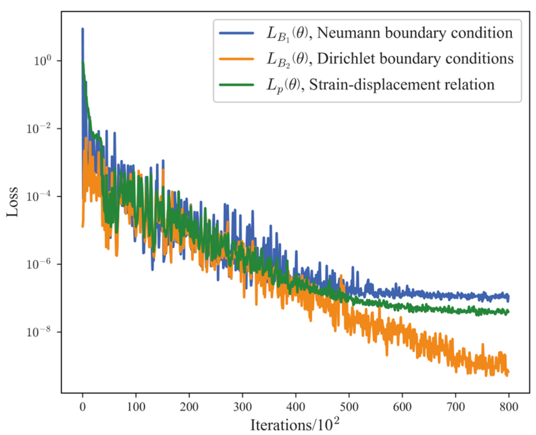
To construct the training datasets for each individual loss, 1000 random strain functions ${\epsilon }^r$ were modeled using GRF. After the training datasets had been constructed, 80,000 iterations of gradient descent were performed to train the PI_DeepONet. The convergence process of each physics-driven loss is shown in Figure 6. The PI_DeepONet converged to the solution operator of the GDEs by minimizing each individual physics-driven loss of GDEs to less than ${10}^{-6}$.

Figure 6. Convergence process of each loss when training the PI_DeepONet for the beam with one end clamped.

Similarly, for the beam with other restrictions, a corresponding PI_DeepONet was built and trained to reconstruct the displacement. For the beam with the restrictions of clamped–clamped, the Neumann boundary conditions at both ends of the beam need to be fitted simultaneously by the PI_DeepONet, resulting in complex loss terms. In this scenario, to mitigate the imbalance between the gradients of each loss throughout the training process, Algorithm 1 was used to perform gradient descent iterations. Recording the updated weights every 100 iterations, the convergent evolutions of the weights when training the PI_DeepONet are summarized in Figure 7.

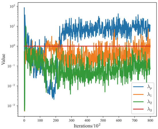
Figure 7. Convergent evolution of the weight of the each physics-driven loss when training the PI_DeepONet for the beam with two ends clamped using Algorithm 1: ${\lambda }_p$ denotes the weight of loss of strain–displacement relation, ${\lambda }_1$ and ${\lambda }_2$ denote the weights of the loss of Neumann boundary conditions at point $x$ = 0 m and $x$ = 1 m, respectively, and ${\lambda }_3$ denotes the weight of the loss of Dirichlet boundary conditions.

For the beam, it is also important to reconstruct rotating angle $\beta$ of the cross-section (see Figure 1). In the case of small displacements, rotating angle $\beta$ can be calculated by taking the first-order derivative of the displacement with respect to coordinate $x$. The displacement is the output of the PI_DeepONet, and coordinate $x$ is one of the inputs. Thus, after inputting strain function ${\epsilon }_i$ and coordinate $x_j$, rotating angle $\beta$ at coordinate $x_j$ can be calculated via PI_DeepONet as follows:

$$\beta =\frac{d{G}_{\theta }\left({\epsilon }_i\right)\left(x_j\right)}{dx}$$

(40)

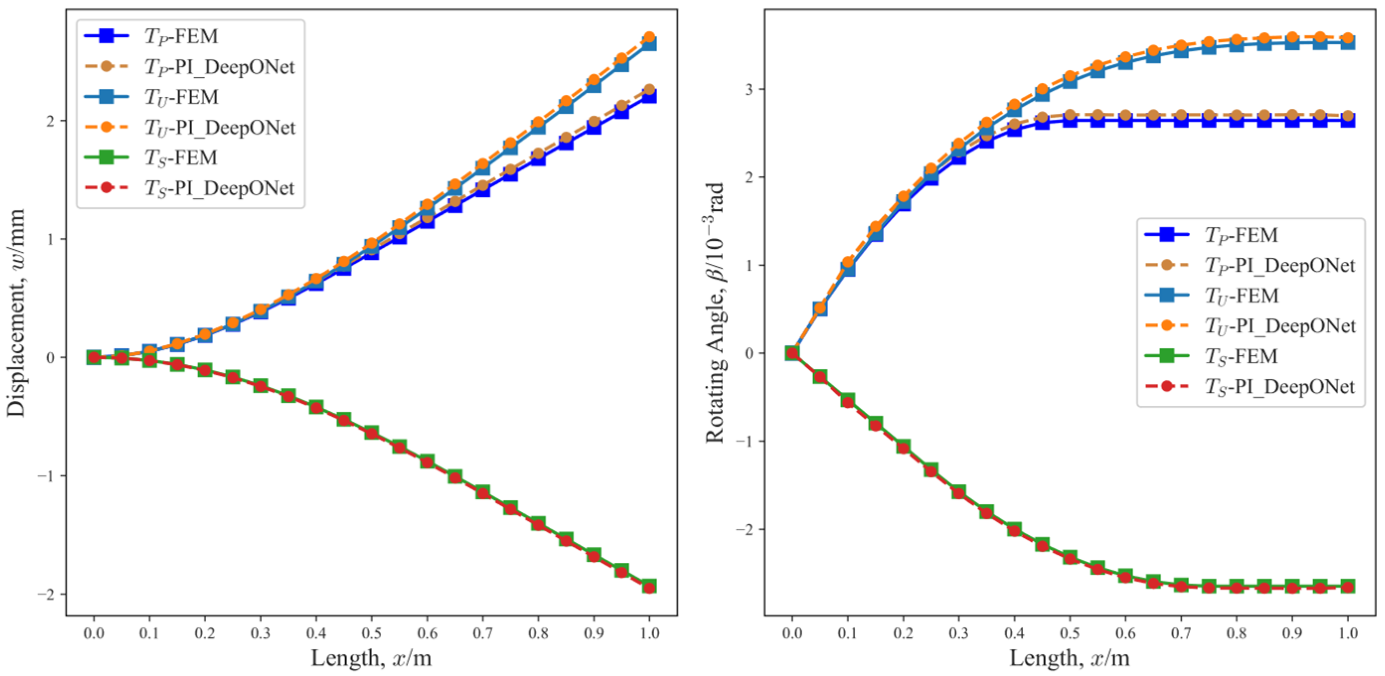
In order to evaluate the performance of the PI_DeepONet, the reconstructed displacement and rotating angle of the beam under three loading conditions were compared to those simulated by FEM. The magnitude and position of each load applied to the beam are shown in Table 2, in which $T_P$ denotes a point force applied at a certain location, $T_U$ denotes uniform pressure applied to the surface of the structure, and $T_S$ denotes two point forces acting in opposite directions at different locations. The reconstruction results of the PI_DeepONet are shown in Figure 8, Figure 9, Figure 10 and Figure 11, in which the $x$ coordinates of displacement and the rotating angle measurement points are ${\left\{0.05\left(i-1\right)\right\}}_{i=1}^{21}$ (m). The fitting accuracy, indicating the degree of agreement between the reconstructed terms and the simulated terms, was used to evaluate the performance of PI_DeepONet. The fitting accuracies of PI_DeepONet for the beam with different restrictions are shown in Table 3. The results show that the reconstructed displacement and rotating angle are basically consistent with the simulated results, and the fitting accuracies are all above 0.99. The results verify the excellent performance of the PI_DeepONet on the reconstruction of displacement and rotating angle for beam. Furthermore, no strain measuring points are positioned at the boundaries ($x=0$ m and $x=1$ m) of the beam, demonstrating that our method is not reliant on the full-field strain.

Table 2. Loads applied to the beam.

Loading Conditions	Magnitude and Position of Each Load
Point load $T_P$	300 N at $x$ = 0.5 m
Uniform pressure $T_U$	0.01 Mpa on the upper surface of the beam
Staggered load $T_S$	150 N at = 0.25 m; −150 N at $x$ = 0.75 m

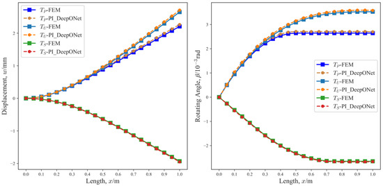
Figure 8. Reconstruction results of the displacement and rotating angle of the beam with one end clamped under different loading conditions.

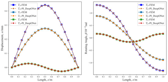
Figure 9. Reconstruction results of the displacement and rotating angle of the beam with the restrictions of simply supported–simply supported under different loading conditions.

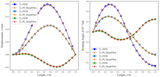
Figure 10. Reconstruction results of the displacement and rotating angle of the beam with the restrictions of clamped–simply supported under different loading conditions.

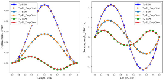
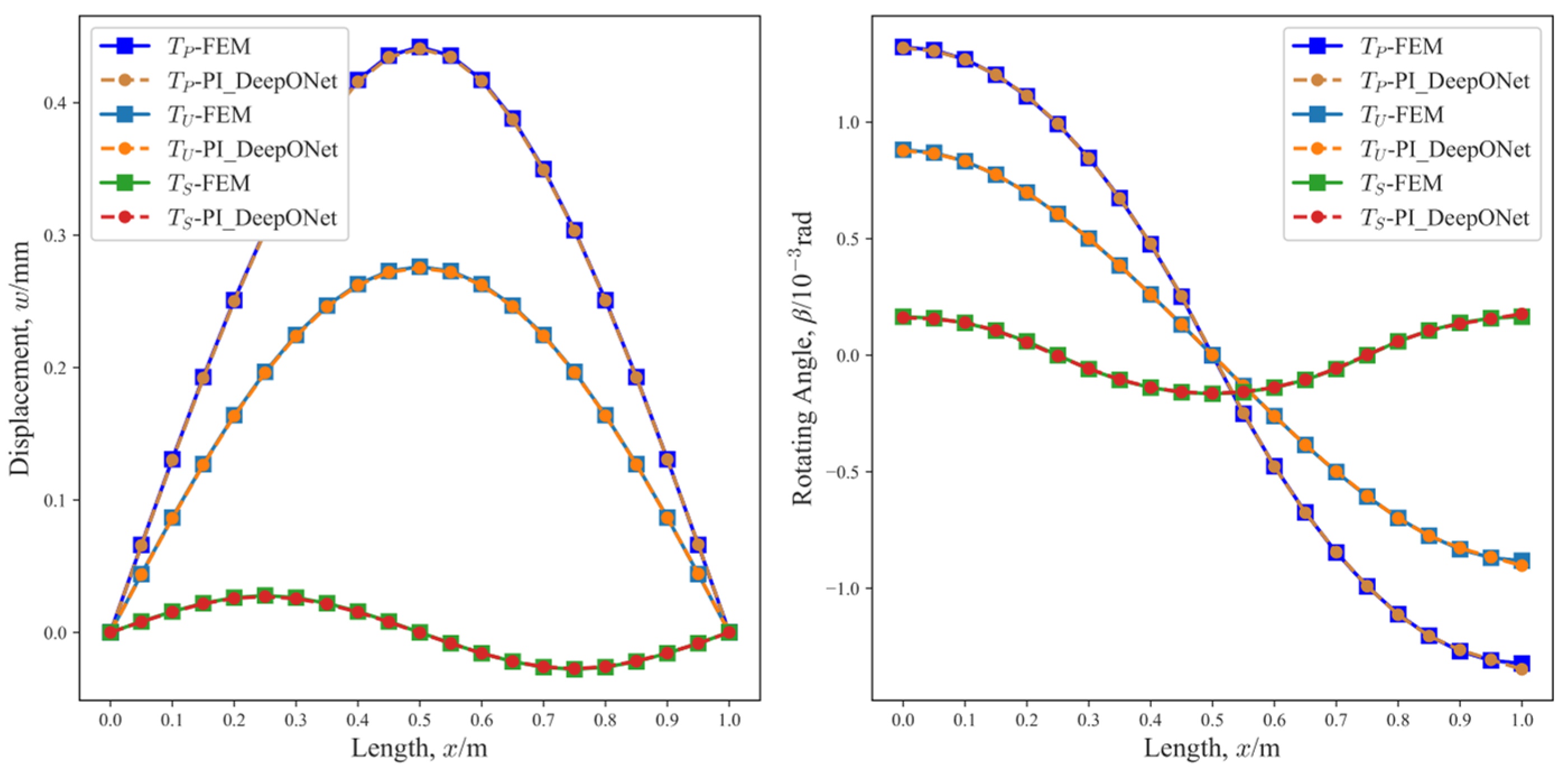
Figure 11. Reconstruction results of the displacement and rotating angle of the beam with the restrictions of clamped–clamped under different loading conditions.

Table 3. Fitting accuracy of the PI_DeepONet for the beam.

Restrictions	Displacement Fitting Accuracy			Rotating Angle Fitting Accuracy
	${\mathit{T}}_{\mathit{P}}$	${\mathit{T}}_{\mathit{U}}$	${\mathit{T}}_{\mathit{S}}$	${\mathit{T}}_{\mathit{P}}$	${\mathit{T}}_{\mathit{U}}$	${\mathit{T}}_{\mathit{S}}$
one end clamped	0.9979	0.9984	0.9996	0.9937	0.9965	0.9993
simply supported–simply supported	0.9999	0.9999	0.9996	0.9999	0.9999	0.9993
clamped–simply supported	0.9997	0.9998	0.9979	0.9997	0.9992	0.9959
clamped–clamped	0.9998	0.9999	0.9962	0.9997	0.9995	0.9973

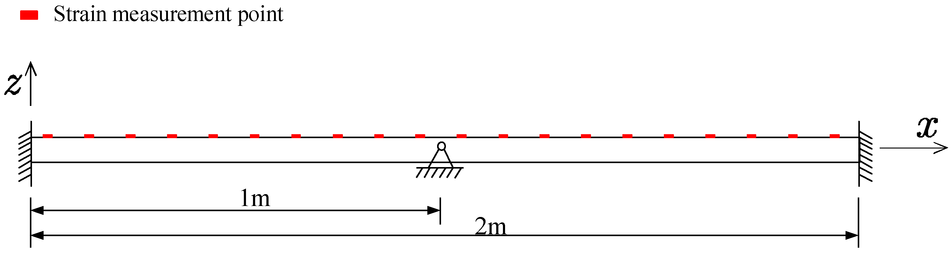
4.1.2. Displacement Reconstruction for Multi-Span Beam

The performance of PI_DeepONet was also evaluated for the multi-span beam. Figure 12 shows the geometric model of the multi-span beam with the restrictions of clamped–simply supported–clamped. There are 20 strain measuring points arranged on the surface of the multi-span beam to reconstruct the displacement and rotating angle. The $x$ coordinates of the strain measuring points are ${\left\{0.02+0.01\left(i-1\right)\right\}}_{i=1}^{20}$ (m). We reconstructed the displacement and rotating angle for the multi-span beam with three boundaries: clamped–simply supported–clamped, clamped–simply supported–simply supported and three points simply supported.

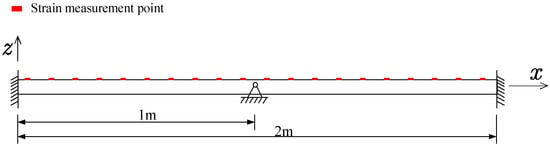
Figure 12. Geometric model of the multi-span beam with the restrictions of clamped–simply supported–clamped.

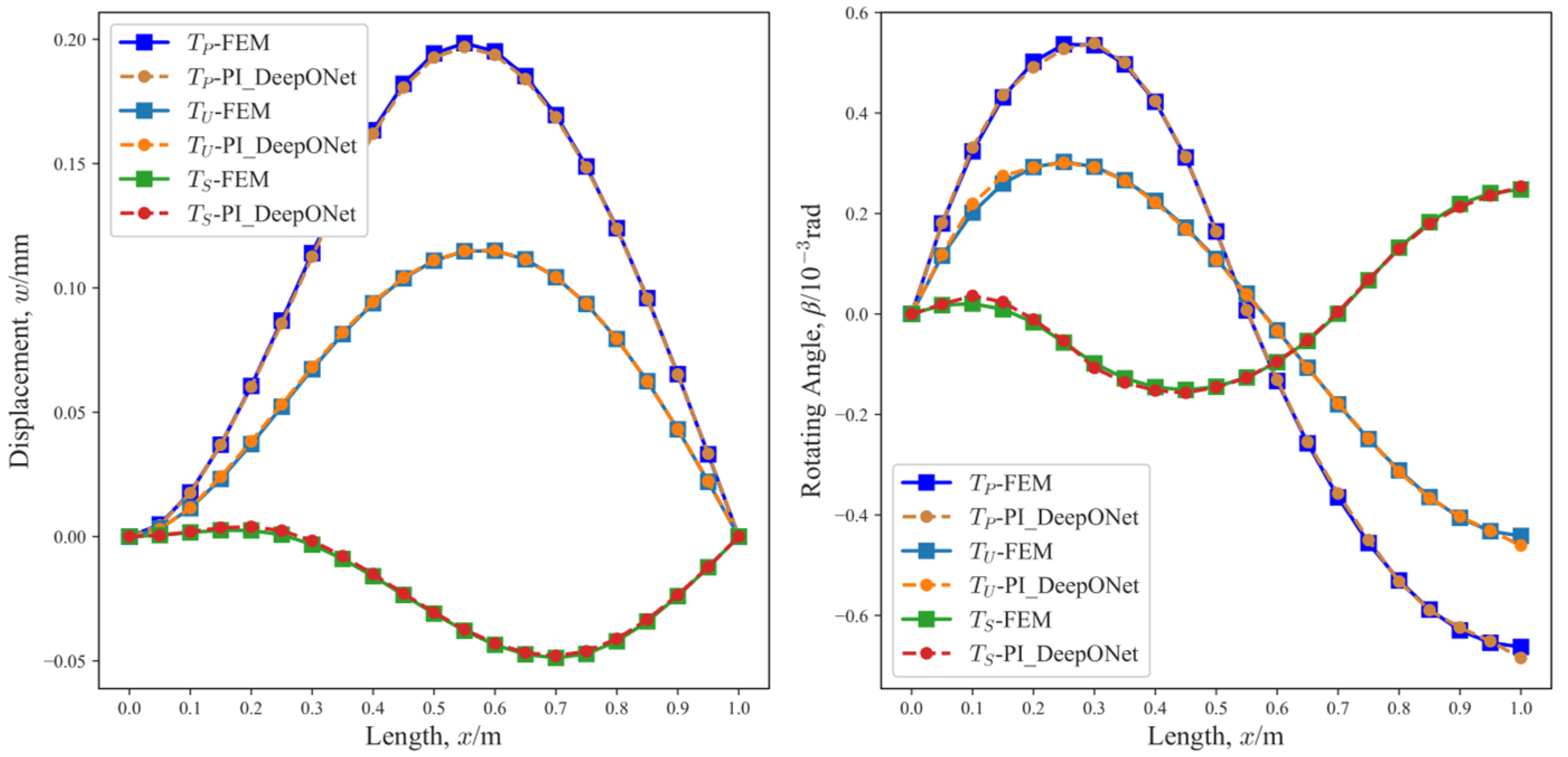
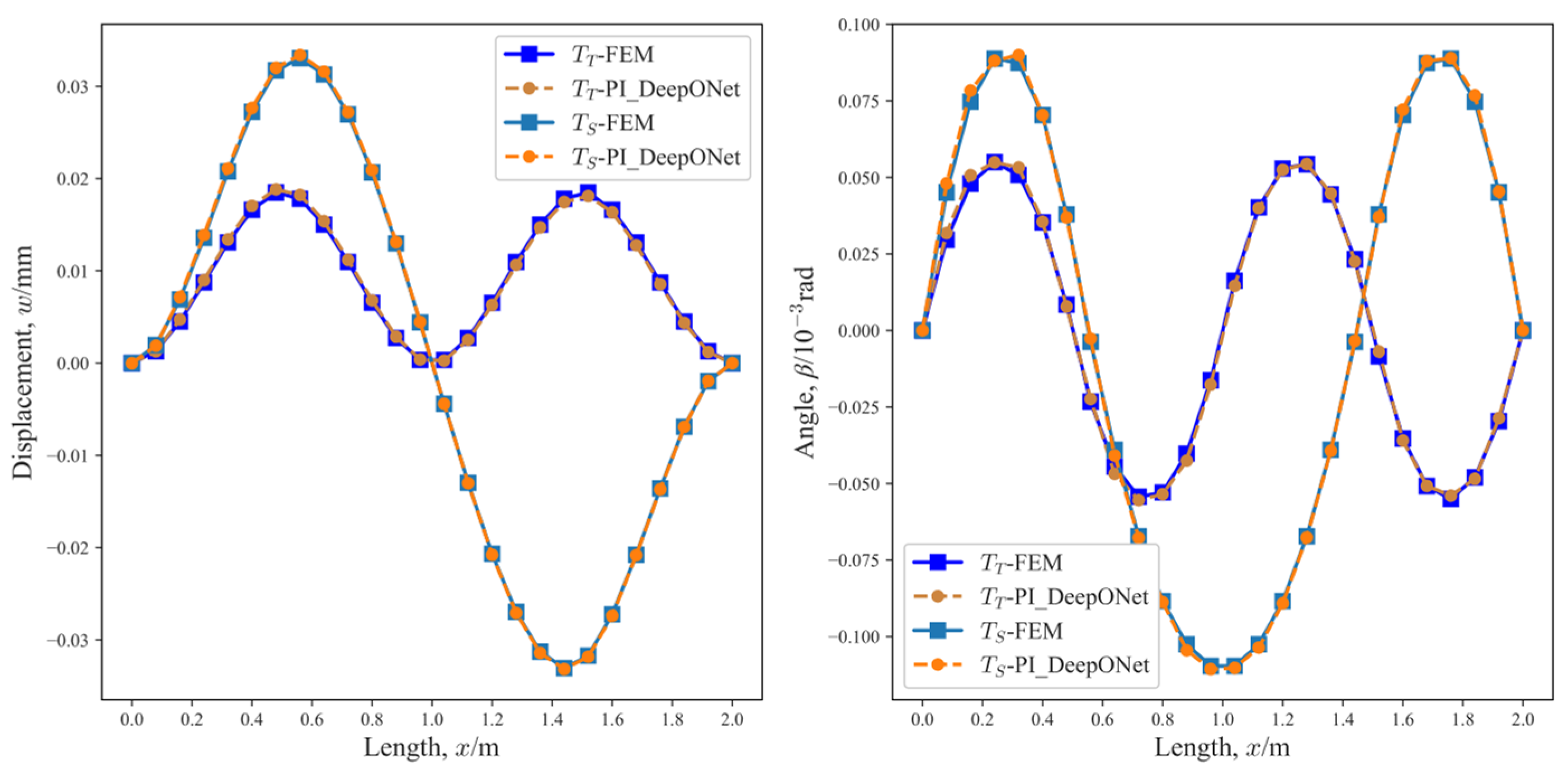
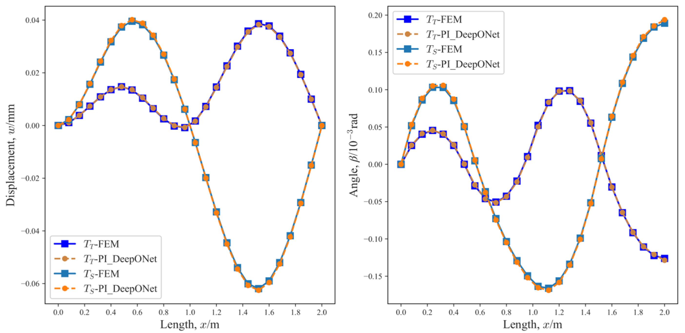
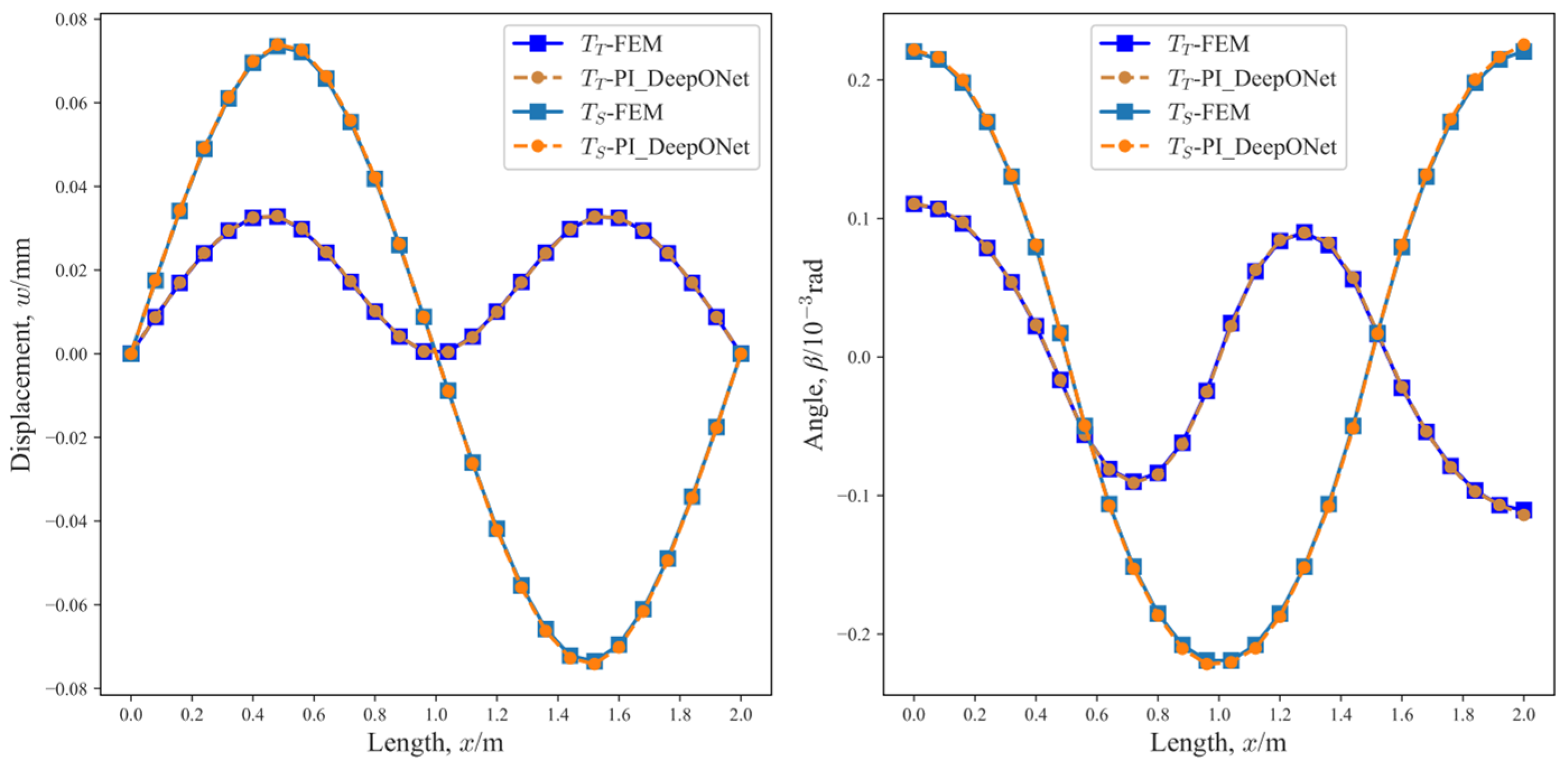
Table 4 shows the magnitude and position of the loads applied to the multi-span beam, in which $T_T$ denotes two point forces acting in the same direction but at different locations. Figure 13, Figure 14 and Figure 15 show the reconstruction results of the PI_DeepONet evaluated at $x$ coordinates ${\left\{0.08\left(i-1\right)\right\}}_{i=1}^{26}$ (m). The fitting accuracies are summarized in Table 5. Based on the reconstruction results, it is evident that the PI_DeepONet can accurately reconstruct the displacement and rotating angle of the multi-span beam.

Table 4. Loads applied to the multi-span beam.

Loading Conditions	Magnitude and Position of Each Load
Two-point loads $T_T$	5 N at $x$ = 0.5 m; 5 N at $x$ = 1.5 m
Staggered load $T_S$	5 N at $x$ = 0.5 m; −5 N at $x$ = 1.5 m

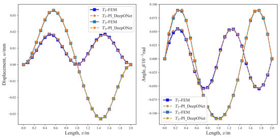
Figure 13. Reconstruction results of the displacement and rotating angle of the multi-span beam with the restrictions of clamped–simply supported–clamped.

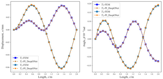
Figure 14. Reconstruction results of the displacement and rotating angle of the multi-span beam with the restrictions of clamped–simply supported–simply supported.

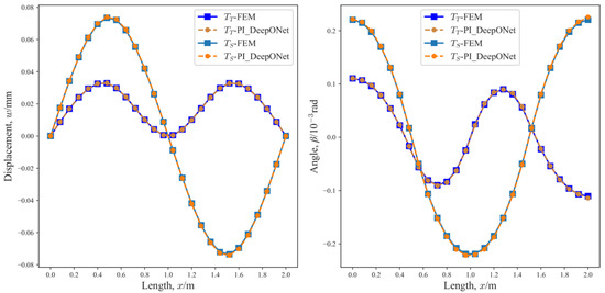
Figure 15. Reconstruction results of the displacement and rotating angle of the multi-span beam with the restrictions of three points simply supported.

Table 5. Fitting accuracy of the PI_DeepONet for the multi-span beam.

Restrictions	Displacement Fitting Accuracy		Rotating Angle Fitting Accuracy
	${\mathit{T}}_{\mathit{T}}$	${\mathit{T}}_{\mathit{S}}$	${\mathit{T}}_{\mathit{T}}$	${\mathit{T}}_{\mathit{S}}$
clamped–simply supported–clamped	0.9983	0.9999	0.9986	0.9994
clamped–simply supported–simply supported	0.9998	0.9998	0.9998	0.9997
three points simply supported	0.9999	0.9999	0.9998	0.9998

4.2. Plate

The reconstruction performance of PI_DeepONet is evaluated in this section using a rectangular plate with various restrictions and a cantilevered triangle plate with variable thickness. The plates with an elastic modulus of 210 Gpa and a Poisson’s ratio of 0.3 were simulated by the finite element analysis software ANSYS2021R1.

4.2.1. Displacement Reconstruction for Rectangular Plate

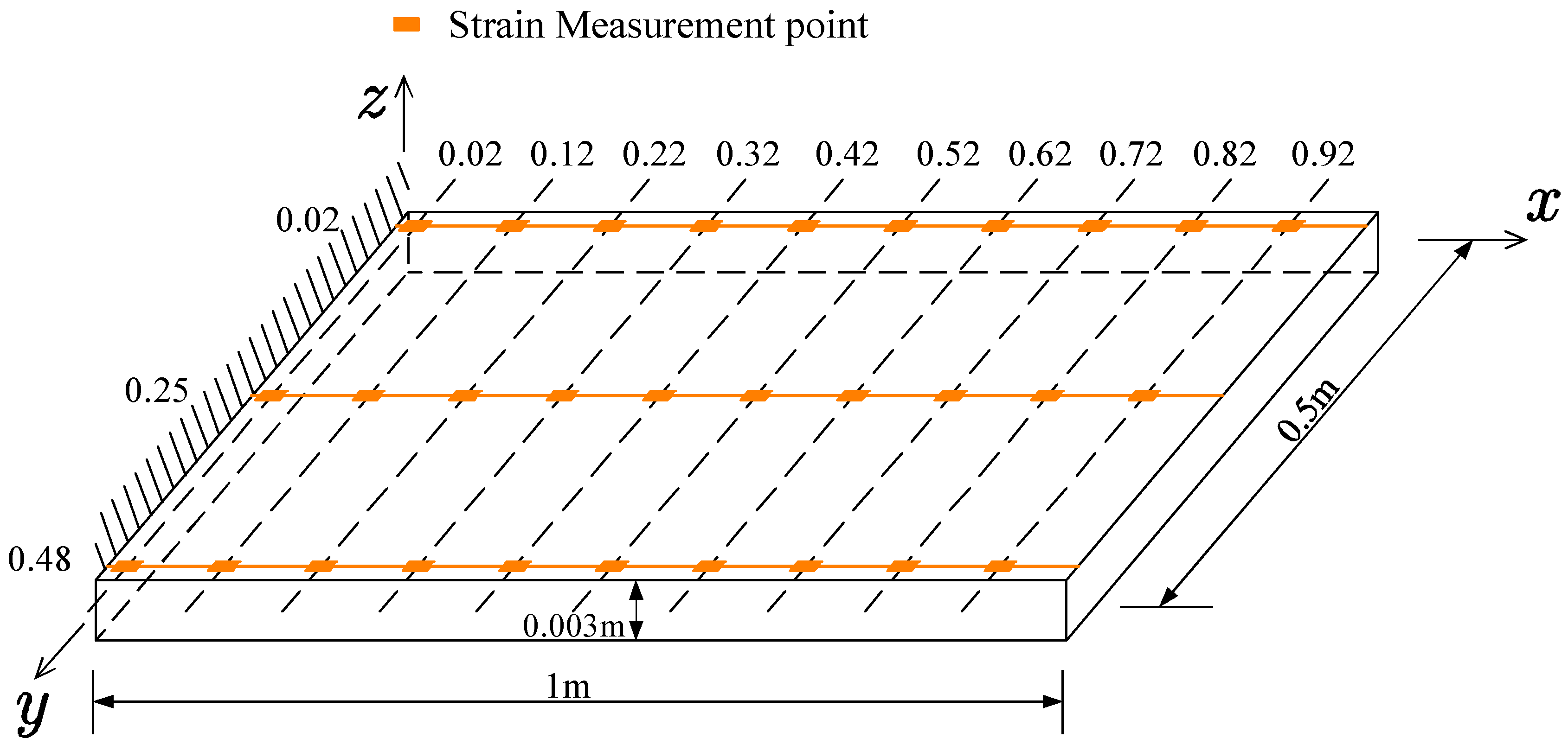
In this section, a rectangular thin plate is utilized to verify the reconstruction performance of PI_DeepONet. The plate is restricted at two opposite sides and free on the remaining two sides. The restrictions applied to the plate are one side clamped, simply supported-simply supported, clamped-simply supported, and clamped-clamped, respectively. Figure 16 shows the geometric model of the plate with one side clamped. There are 30 strain measuring points arranged on the three parallel lines along the $x$ coordinate direction. The $y$ coordinates of the three parallel lines are (0.02 m, 0.25 m, 0.48 m), respectively. The $x$ coordinates of the strain measuring points on each line are ${\left\{0.02+0.01\left(i-1\right)\right\}}_i^{10}$ (m). All the arranged measuring points modeling FBG-based strain gauges detect the strain in the $x$ coordinate direction.

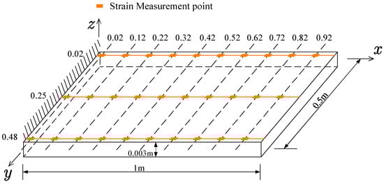
Figure 16. The geometric model of the plate with one side clamped.

The strain–displacement relation and restrictions along three parallel lines share the GDEs of the unified form. The GDEs along the parallel lines were used for formulating the physics losses for PI_DeepONet. For plates with different restrictions, a corresponding PI_DeepONet was built and trained separately to reconstruct the displacement.

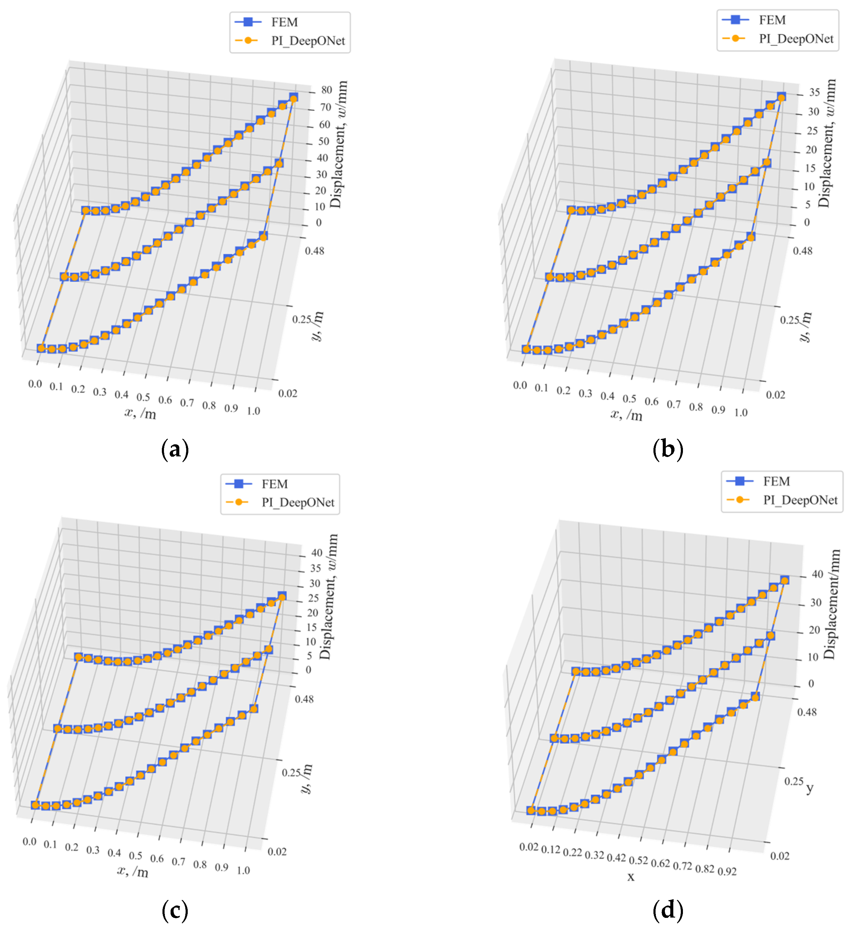
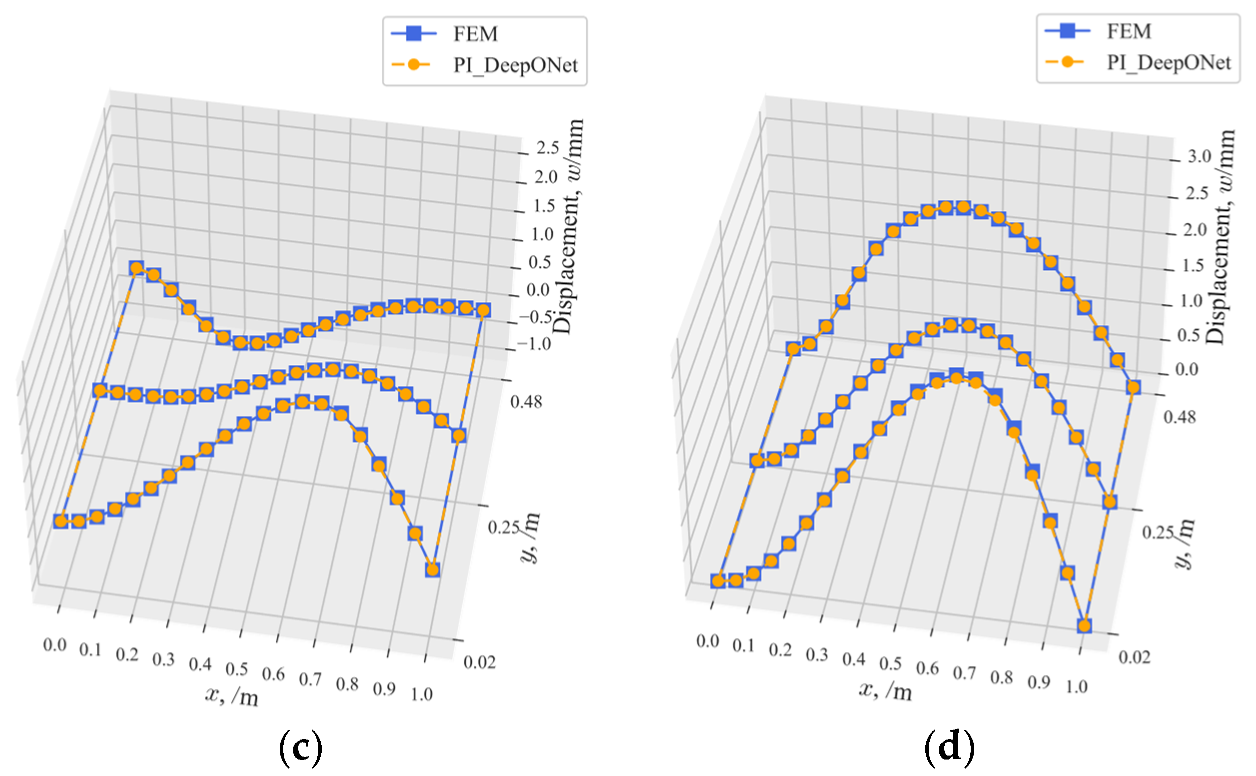
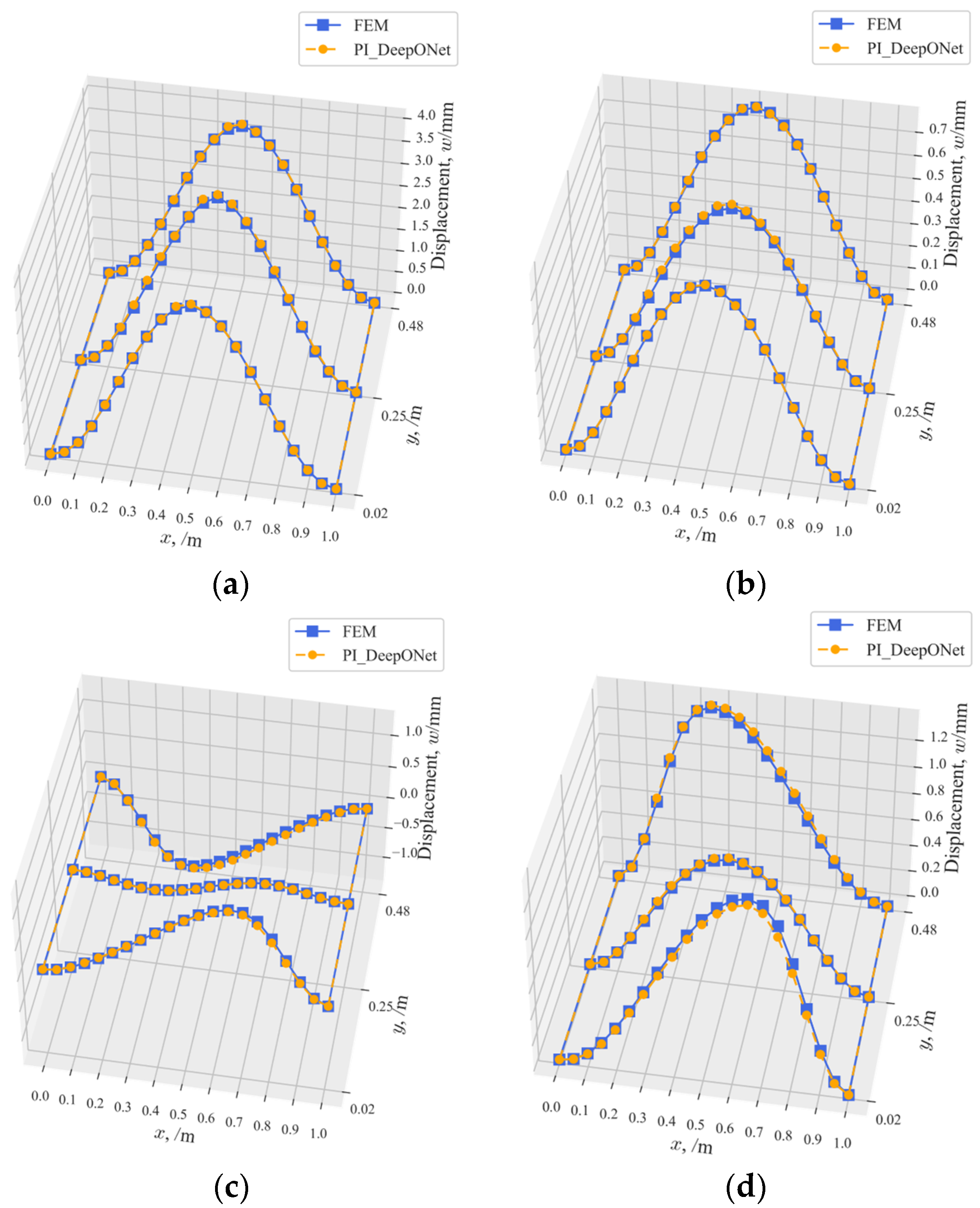
The strain and displacement were simulated by FEM under four loading conditions. The loads applied to the plate are shown in Table 6. Inputting the simulated strain and the coordinate of displacement measuring point on each line, the reconstructed displacement at the displacement measuring point can be outputted by the PI_DeepONet. The $x$ coordinates of the displacement measuring points on each line are ${\left\{0.05\left(i-1\right)\right\}}_{i=1}^{21}$ (m). The reconstructed displacement was compared with the FEM-simulated one and the results are shown in Figure 17, Figure 18, Figure 19 and Figure 20. The fitting accuracy of the PI_DeepONet for the plate is shown in Table 7. The results indicate that the reconstructed displacement generally matches the FEM-simulated displacement, which demonstrates the broad applicability of PI_DeepONet.

Table 6. Loads applied to the plate.

Loading Conditions	Magnitude and Position of Each Load
Point load $T_P$	200 N at ($x$ = 0.5 m, $y$ = 0.25 m)
Uniform pressure $T_U$	150 Pa on the upper surface
Staggered loads $T_S$	50 N at ($x$ = 0.75 m, $y$ = 0 m); −50 N at ($x$ = 0.25 m, $y$ = 0.5 m)
Two-points loads $T_T$	50 N at ($x$ = 0.75 m, $y$ = 0 m); 50 N at ($x$ = 0.25 m, $y$ = 0.5 m)

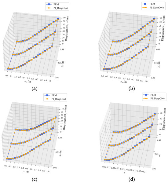
Figure 17. Reconstruction results of the displacement for the plate with one side clamped under different loading conditions: (a) reconstruction results under loading condition $T_P$, (b) reconstruction results under loading condition $T_U$, (c) reconstruction results under loading condition $T_S$, and (d) reconstruction results under loading condition $T_T$.

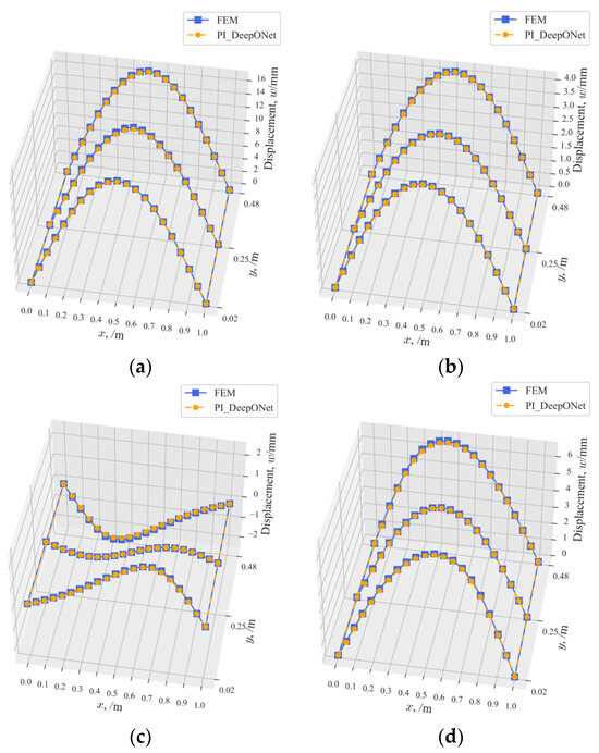
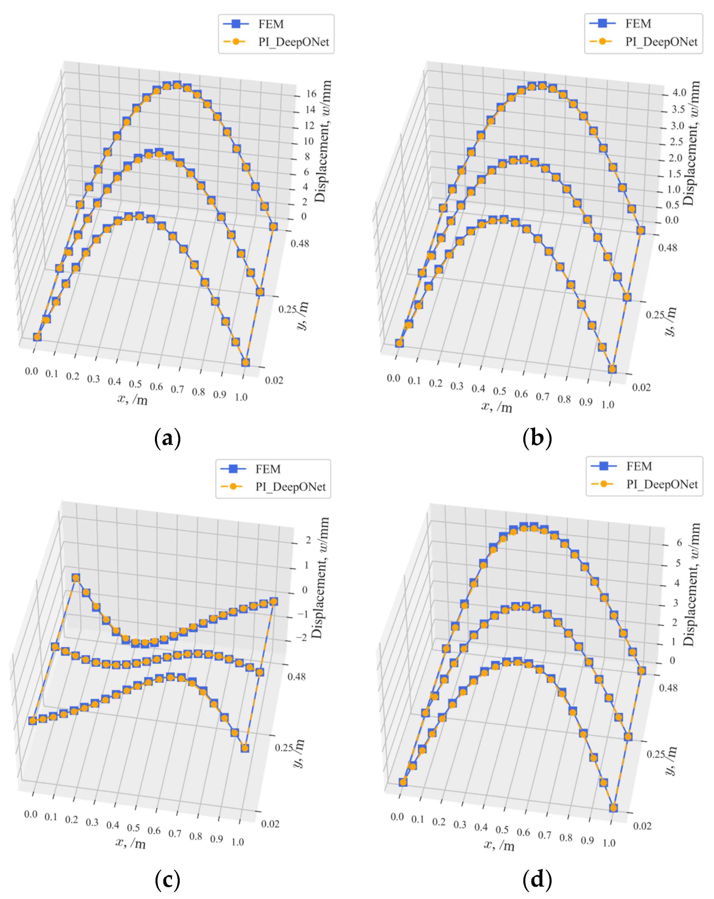
Figure 18. Reconstruction results of the displacement for the plate with two sides simply supported under different loading conditions: (a) reconstruction results under loading condition $T_P$, (b) reconstruction results under loading condition $T_U$, (c) reconstruction results under loading condition $T_S$, and (d) reconstruction results under loading condition $T_T$.

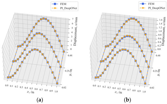
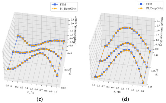
Figure 19. Reconstruction results of the displacement for the plate with one side clamped and one side simply supported under different loading conditions: (a) reconstruction results under loading condition $T_P$, (b) reconstruction results under loading condition $T_U$, (c) reconstruction results under loading condition $T_S$, and (d) reconstruction results under loading condition $T_T$.

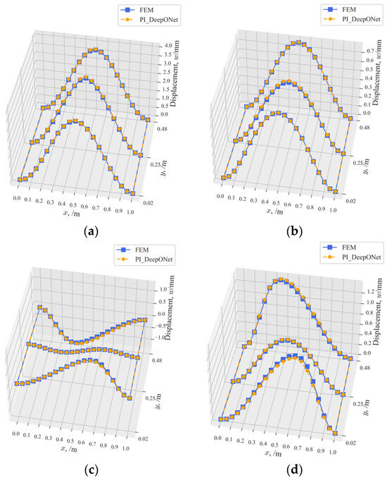
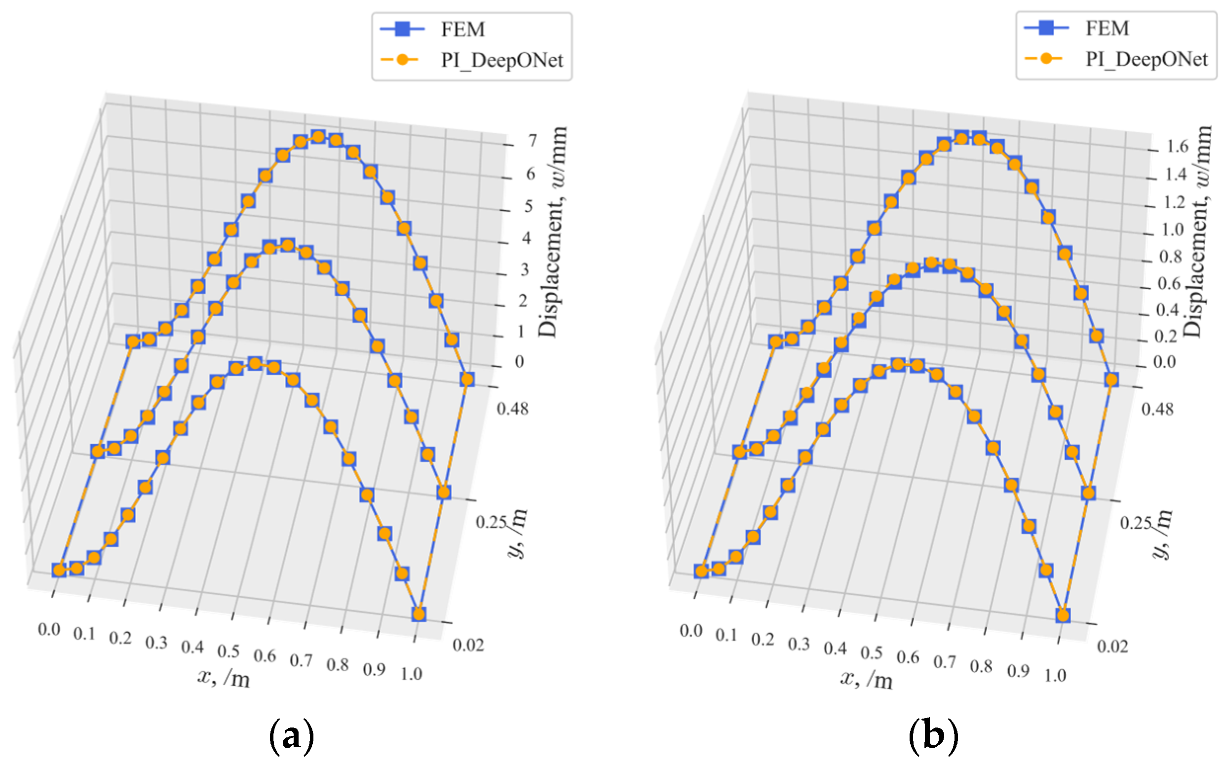
Figure 20. Reconstruction results of the displacement for the plate with two sides clamped under different loading conditions: (a) reconstruction results under loading condition $T_P$, (b) reconstruction results under loading condition $T_U$, (c) reconstruction results under loading condition $T_S$, and (d) reconstruction results under loading condition $T_T$.

Table 7. Fitting accuracy of the PI_DeepONet for the plate.

Restrictions	Displacement Fitting Accuracy
	${\mathit{T}}_{\mathit{P}}$	${\mathit{T}}_{\mathit{U}}$	${\mathit{T}}_{\mathit{S}}$	${\mathit{T}}_{\mathit{T}}$
one side clamped	0.9995	0.9996	0.9996	0.9997
simply supported–simply supported	0.9991	0.9995	0.9991	0.9989
clamped–simply supported	0.9999	0.9996	0.9997	0.9994
clamped–clamped	0.9995	0.9993	0.9984	0.9966

4.2.2. Displacement Reconstruction for Triangle Plate with Variable Thickness

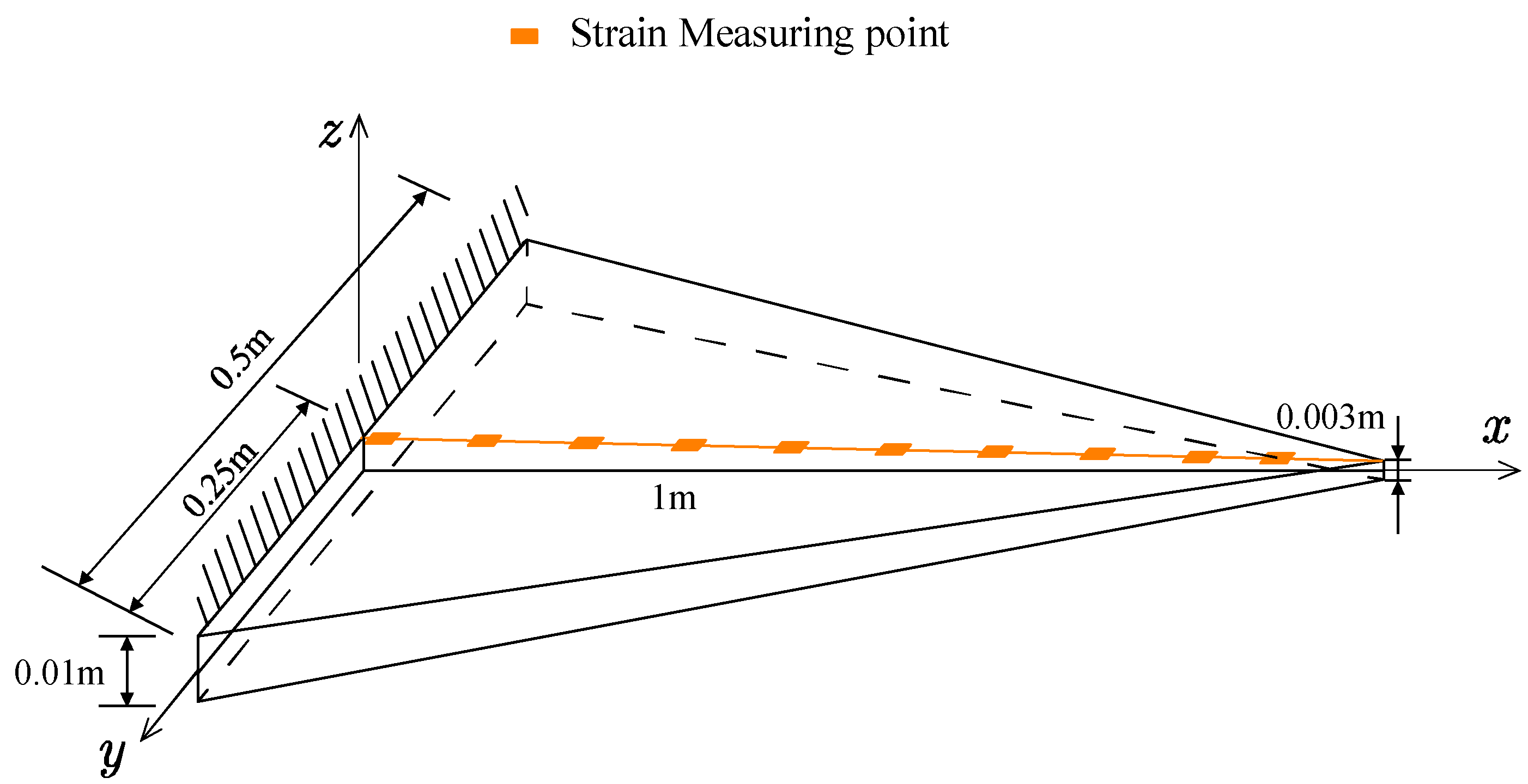
In this section, the displacement of a cantilevered triangle plate with variable thickness is reconstructed by PI_DeepONet. The geometric model of the triangle plate is shown in Figure 21. The thickness of the triangular plate varies linearly in the $x$ direction. We arranged 10 strain measuring points on the centerline of the upper surface to reconstruct the corresponding displacement. The $x$ coordinates of the strain measuring points are ${\left\{0.02+0.01\left(i-1\right)\right\}}_{i=1}^{10}$ (m).

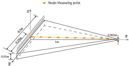
Figure 21. The geometric model of the cantilevered triangle plate with variable cross-section.

Since the thickness of the plate is variable, the strain–displacement relation described in Equation (7) should be updated as follows

$$\{\begin{array}{l}{\epsilon }_x\left(x,y\right)=-0.5t\left(x\right)\frac{{\partial }^{2}w\left(x,y\right)}{\partial x^2}\hfill \\ {\epsilon }_y\left(x,y\right)=-0.5t\left(x\right)\frac{{\partial }^{2}w\left(x,y\right)}{\partial y^2}\hfill \end{array}$$

(41)

in which $t\left(x\right)=-0.007x+0.01$ (m) for the triangle plate shown in Figure 21.

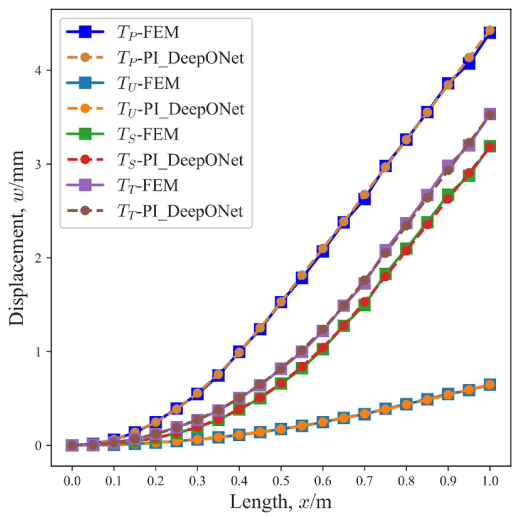
Using the GDEs of the cantilevered triangle plate as the loss terms, the PI_DeepONet was built and trained. We reconstructed the centerline displacement of the triangle plate under four loading conditions via PI_DeepONet. The loads applied to the triangle plate are shown in Table 8. The $x$ coordinates of the location where the displacements were reconstructed are ${\left\{0.05\left(i-1\right)\right\}}_{i=1}^{21}$ (m). Figure 22 shows the curves of the reconstructed displacements and the simulated ones. The fitting accuracies of the PI_DeepONet for the cantilevered triangle plate are summarized in Table 9. The fitting accuracies under four loading conditions are all above 0.99, indicating the excellent agreement between the reconstructed displacements and the FEM-simulated results.

Table 8. Loads applied to the triangle plate with variable thickness.

Loading Conditions	Magnitude and Position of Each Load
Point load $T_P$	100 N at (= 0.5 m, $y$ = 0 m)
Uniform pressure $T_U$	150 Pa on the upper surface
Staggered loads $T_S$	50 N at ($x$ = 0.75 m, $y$ = −0.0625 m); −50 N at ($x$ = 0.25 m, $y$ = 0.1875 m)
Two-point loads $T_T$	50 N at ($x$ = 0.75 m, $y$ = −0.0625 m); 50 N at ($x$ = 0.25 m, $y$ = 0.1875 m)

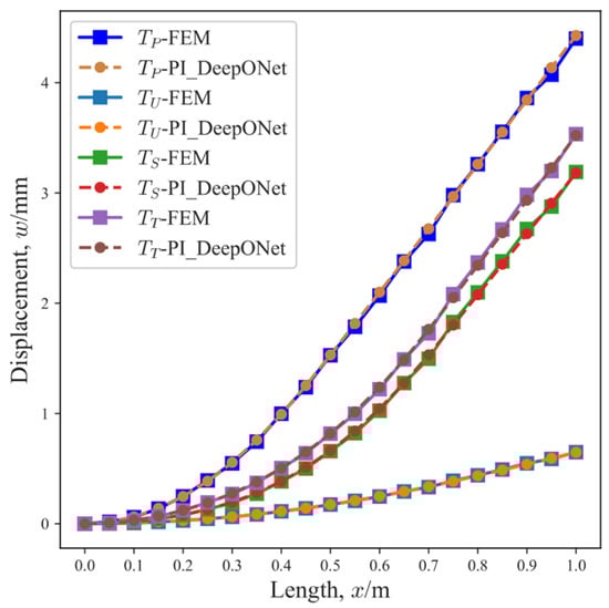
Figure 22. Reconstruction results of the displacement for the triangle plate with variable thickness.

Table 9. Fitting accuracy of the PI_DeepONet for the triangle plate with variable thickness.

Loading Conditions	Displacement Fitting Accuracy
Point load $T_P$	0.9999
Uniform load $T_U$	0.9997
Staggered load $T_S$	0.9998
Two points $T_T$	0.9997

4.3. Discussion

4.3.1. Sensitivity Analysis for Strain Measurement Points

The performance of the strain-based displacement reconstruction methods is significantly affected by the arrangement of strain measurement points. In this section, the sensitivity of the reconstruction accuracy of the PI_DeepONet to the locations and number of strain measurement points is analyzed.

In the numerical examples we presented in Section 4.1 and Section 4.2, the strain measurement points are uniformly distributed and the distance between adjacent strain measurement points is constant. To investigate whether PI_DeepONet relies on uniformly arranged measurement points, we performed the same reconstruction task for the beam via randomly arranged strain measurement points. The relative errors at the maximum response are compared in Table 10. The results show that the reconstructed accuracies for the randomly and uniformly arranged points are essentially consistent, indicating the low sensitivity of PI_DeepONet to the locations of strain measurement points.

Table 10. Relative errors in the maximum response calculated by the PI_DeepONet via uniformly arranged measurement points and randomly arranged measurement points for the beam with different restrictions.

Restrictions	Relative Errors
	Uniformly Arranged Strain Measurement Points			Randomly Arranged Strain Measurement Points
	${\mathit{T}}_{\mathit{P}}$	${\mathit{T}}_{\mathit{U}}$	${\mathit{T}}_{\mathit{S}}$	${\mathit{T}}_{\mathit{P}}$	${\mathit{T}}_{\mathit{U}}$	${\mathit{T}}_{\mathit{S}}$
one end clamped	2.5%	2.2%	1.0%	2.7%	1.4%	0.055%
simply supported–simply supported	0.32%	0.29%	2.9%	0.78%	0.013%	1.1%
clamped–simply supported	0.78%	0.013%	1.7%	1.1%	0.024%	1.3%
clamped–clamped	1.0%	0.088%	0.74%	0.30%	0.44%	1.1%

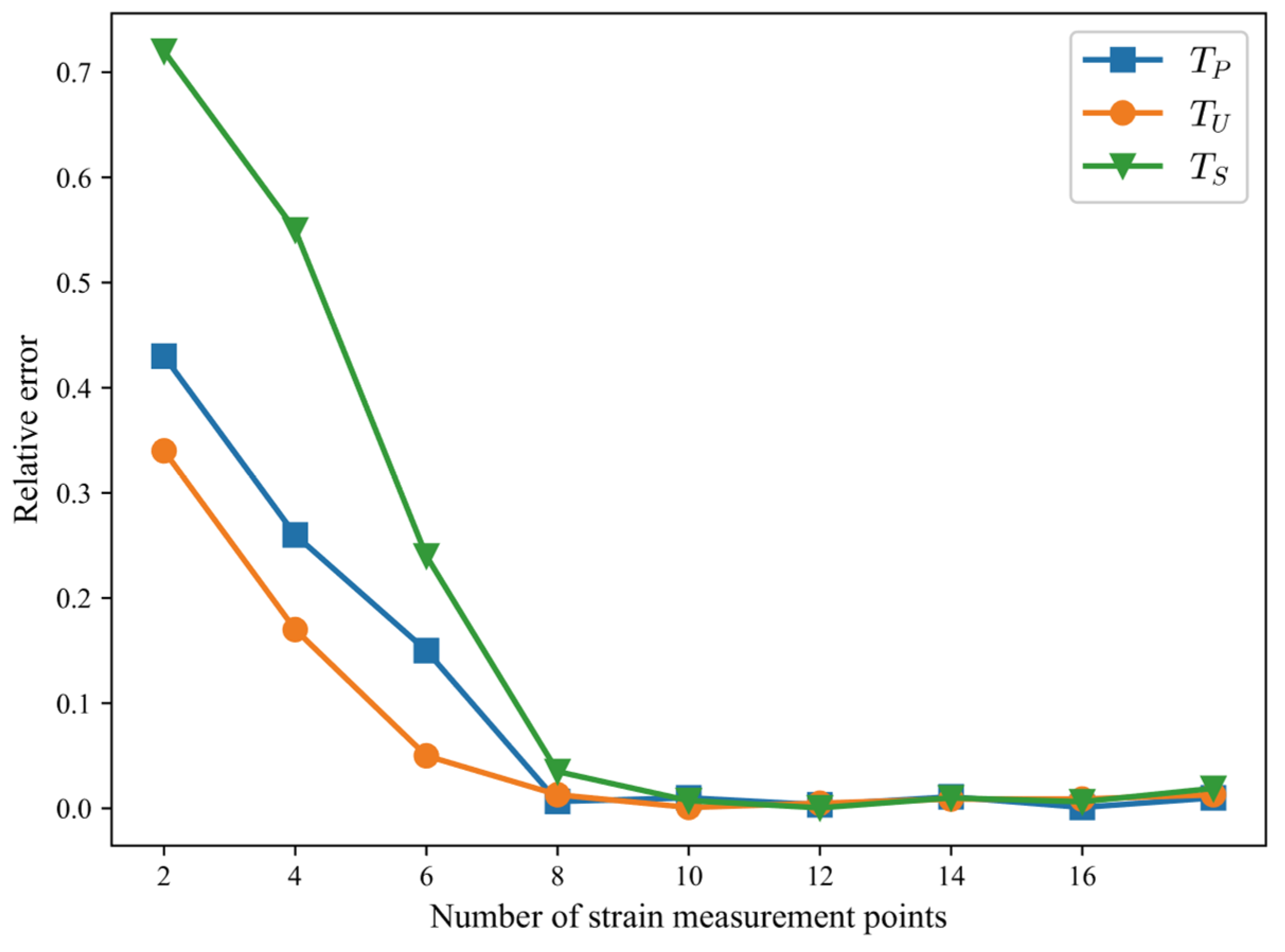
The sensitivity of the reconstruction accuracy of PI_DeepONet to the number of strain measurement points was analyzed utilizing the beam with two ends clamped. The reconstruction accuracy of the PI_DeepONet was evaluated for the number of strain measurement points ranging from 2 to 18. The evolution of the relative error at the maximum response with the number of measurement points is shown in Figure 23. The results show that the relative error decreases as the number of measurement points increases. However, the relative error remains stable after the number of measurement points exceeds a certain threshold. The threshold of the number of strain measurement points for the complex load is higher than that for the simple load. Therefore, an adequate number of strain measurement points is essential to perform the reconstruction task via PI_DeepONet.

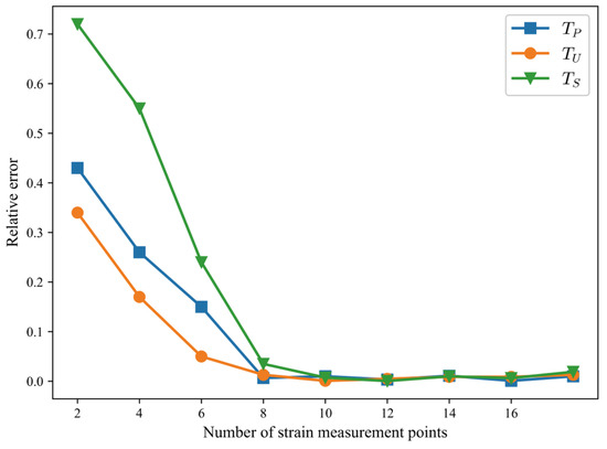
Figure 23. Evolution of the relative error at the maximum response with the number of strain measurement points for the beam with the restriction of two clamped ends.

4.3.2. Ablation Test for Weight-Updating Algorithm

While training the PI_DeepONet for the beam with two ends clamped, the multi-span beam with the restrictions of clamped–simply supported–clamped, and the plate with two sides clamped, as described above, Algorithm 1 was used to perform gradient descent iterations. To demonstrate the superiority of Algorithm 1, ablation tests are performed in this section.

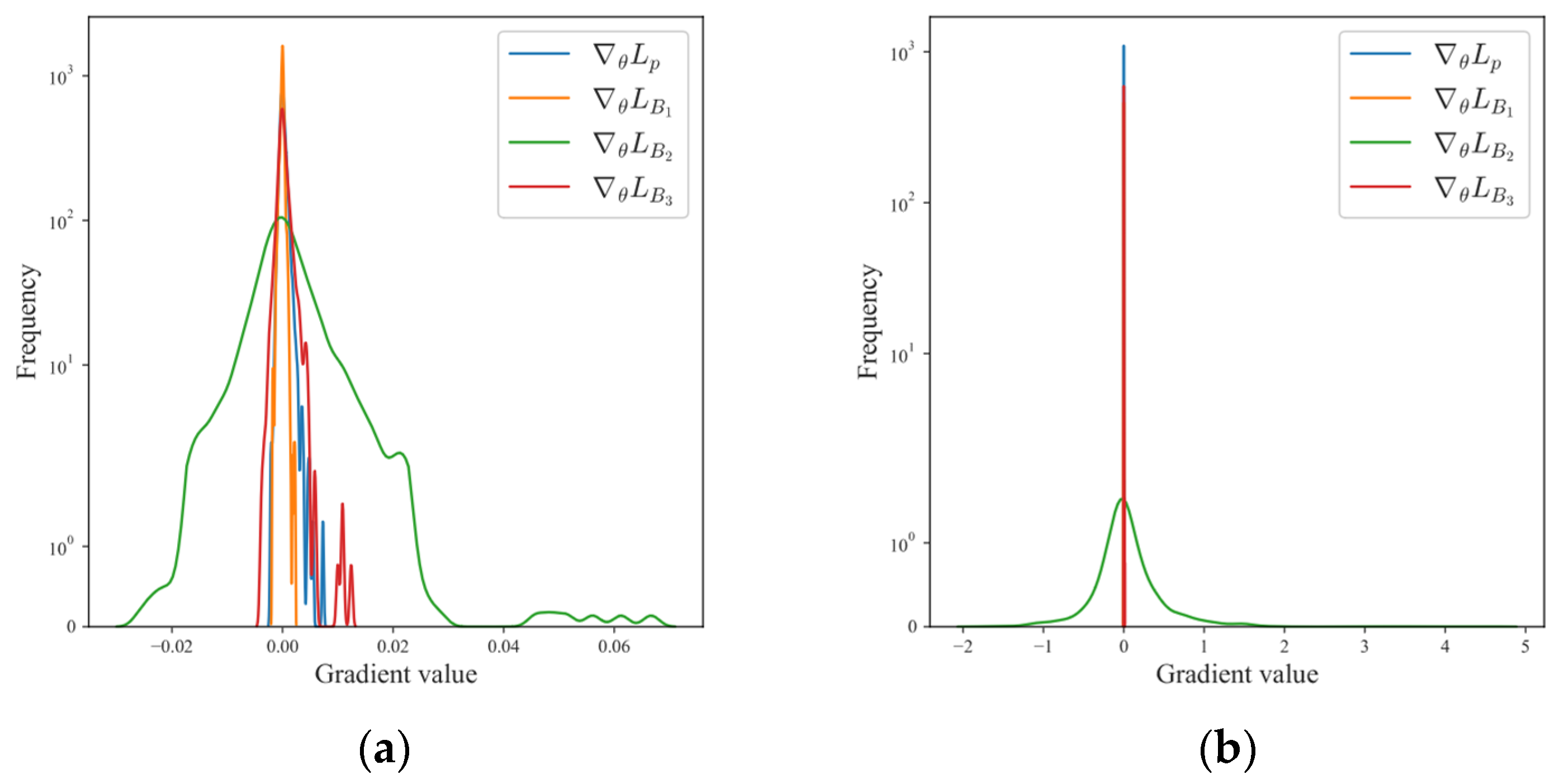
The histograms of the back-propagated gradients of each physics-driven loss with respect to the parameters of the PI_DeepONet at the first layer of the trunk net are shown in Figure 24, Figure 25 and Figure 26. They were monitored after 40,000 iterations. The results indicate that the gradients of $L_{B_2}\left(\theta \right)$ have significantly higher overall values than the gradients of other losses when the updated weights are not applied. This makes it challenging for the PI_DeepONet to evenly fit each loss. Using the weights calculated in Algorithm 1 as the multipliers of each loss, the imbalance in the gradients of each loss is alleviated.

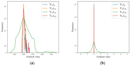
Figure 24. Histograms of back-propagated gradients of each physics-driven loss for the beam with restrictions of clamped–clamped at the first layer of the trunk net after 40,000 training iterations of a PI_DeepONet: (a) histograms of back-propagated gradients with the updated weights applied and (b) histograms of back-propagated gradients with all weights set as 1.

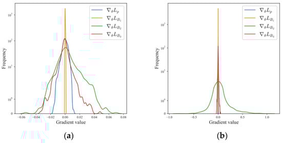
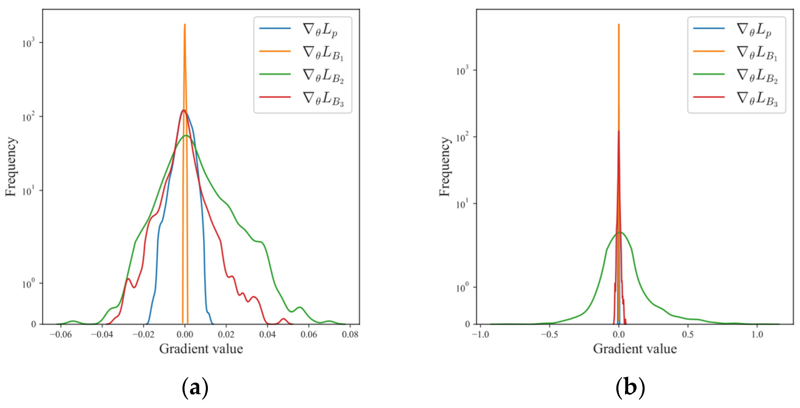
Figure 25. Histograms of back-propagated gradients of each physics-driven loss for the multi-span beam with the restrictions of clamped–simply supported–clamped at the first layer of trunk net after 40,000 iterations of training for PI_DeepONet: (a) histograms of back-propagated gradients with the updated weights applied and (b) histograms of back-propagated gradients with all weights set as 1.

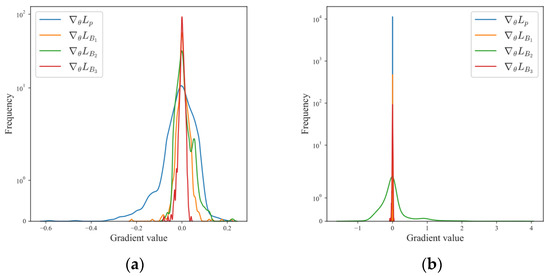
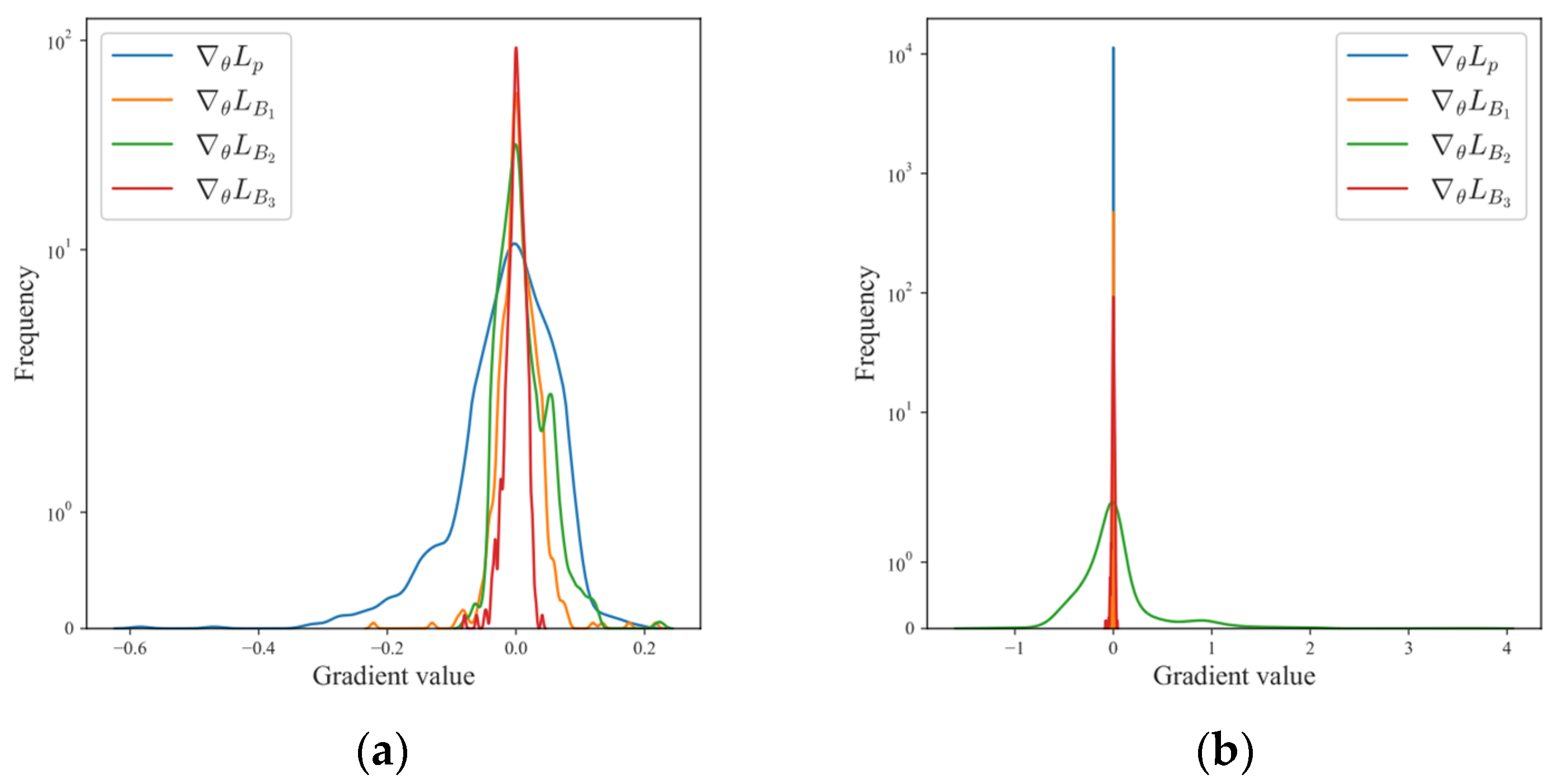
Figure 26. Histograms of back-propagated gradients of each physics-driven loss for the plate with the restrictions of clamped–clamped at the first layer of trunk net after 40,000 iterations of training PI_DeepONet: (a) histograms of back-propagated gradients with the updated weights applied and (b) histograms of back-propagated gradients with all weights set as 1.

For comparison purposes, a PI_DeepONet trained using conventional gradient descent iterations was constructed for each structure with more than one Neumann boundary condition. Additionally, a PI_DeepONet trained using the adaptive weighting method based on Gaussian probabilistic models [38] was also constructed, with the loss function expressed as follows:

$$L\left(\theta \right)=\frac{1}{2{\beta }_p^2}{L}_p\left(\theta \right)+{\displaystyle \sum _{i=1}^{H+1}\frac{1}{2{\beta }_{B_i}^2}{L}_{B_i}\left(\theta \right)+\log \left({\beta }_p{\displaystyle \prod _{i=1}^{H+1}{\beta }_{B_i}}\right)}$$

(42)

where the ${\beta }_p$ and ${\left\{{\beta }_{B_i}\right\}}_{i=1}^{H+1}$ describe the adaptive weights of the loss terms and are tuned via the Adam optimizer before updating the parameters of the network in each gradient descent iteration. The relative errors in the maximum response calculated by the PI_DeepONet trained using the three methods are summarized in Table 11, Table 12 and Table 13. The results show that the algorithm based on Gaussian probabilistic models can improve the reconstruction accuracy of single-span and multi-span beams, but leads to the incorrect convergence of the plate. In contrast, Algorithm 1 has broader applicability and can significantly reduce the relative errors by an order of magnitude. The variables used to update the parameters of the network via gradient descent are gradients of loss terms rather than magnitudes. The gradients and magnitudes of loss terms tend to exhibit completely different distributions. Therefore, it is more logical to balance the interplay among loss terms from the perspective of gradients. This is why our proposed algorithm demonstrates superiority.

Table 11. Relative errors at the maximum response calculated by the PI_DeepONet for the beam with the restrictions of clamped–clamped.

Method	Relative Errors
	${\mathit{T}}_{\mathit{P}}$	${\mathit{T}}_{\mathit{U}}$	${\mathit{T}}_{\mathit{S}}$
Algorithm 1	1.6%	0.64%	3.7%
Gaussian probabilistic models	1.0%	3.4%	33%
Normal gradient descent iterations	31%	40%	55%

Table 12. Relative errors at the maximum response calculated by the PI_DeepONet for the multi-span beam with the restrictions of clamped–simply supported–clamped.

Method	Relative Errors
	${\mathit{T}}_{\mathit{T}}$	${\mathit{T}}_{\mathit{S}}$
Algorithm 1	1.9%	0.35%
Gaussian probabilistic models	2.8%	2.5%
Normal gradient descent iterations	6.1%	3.9%

Table 13. Relative errors at the maximum response calculated by the PI_DeepONet for the plate with the restrictions of clamped–clamped.

Method	Relative Errors
	${\mathit{T}}_{\mathit{P}}$	${\mathit{T}}_{\mathit{U}}$	${\mathit{T}}_{\mathit{S}}$	${\mathit{T}}_{\mathit{T}}$
Algorithm 1	1.3%	0.026%	2.0%	3.2%
Gaussian probabilistic models	27%	26%	64%	57%
Normal gradient descent iterations	9.2%	6.7%	4.2%	21%

4.3.3. Comparison between the PI_DeepONet and Ko Method

The Ko method also reconstructs the displacement by solving the GDEs of the structure. However, the Ko method solves the GDEs by directly integrating the strain function twice, which necessitates a full-field strain. Therefore, the Ko method is not applicable in situations where no strain measuring points are arranged at the boundary, as we demonstrated in Section 4.1 and Section 4.2. In addition, to reconstruct the full-field strain, the Ko method assumes that the strain values between the adjacent strain measurement points are linearly varied, which can lead to a significant reconstruction error in certain scenarios.

Using the beam with the restrictions of clamped–clamped as the example, the reconstruction performance of the two methods was evaluated. The $x$ coordinates of the strain measuring points were set as ${\left\{0.1\left(i-1\right)\right\}}_{i=1}^{11}$ (m). After determining the arrangement of the strain measuring points, PI_DeepONet was built and trained for the displacement reconstruction. The strain and displacement under three loading conditions were simulated by FEM, and the displacement was reconstructed by the two methods, using simulated strain as the input. Table 14 summarizes the relative errors of the two methods at the maximum response. For point load $T_P$, both methods have a high reconstruction accuracy. However, for uniform load $T_U$ and staggered load $T_S$, the reconstruction accuracy of the PI_DeepONet is much higher than that of the Ko method. This is because the Ko method assumes that the strain is linearly varied between neighboring strain measuring points. When the structure is subjected to point load, the strain is linearly distributed, so the Ko method achieves high accuracy in this case. However, the assumption of linearly varied strain is not valid when the structure is subjected to complex loads, such as uniform load and staggered load. Thus, the Ko method results in poor reconstruction accuracy in these scenarios. In contrast to the Ko method, PI_DeepONet can extract information about the full-field strain from discrete strains with the assistance of the powerful nonlinear fitting capability of the neural network. Therefore, PI_DeepONet has high reconstruction accuracy, even under complex loading conditions. Furthermore, our proposed method can directly reconstruct the full-field displacement of the beam, which is not achievable via the Ko method.

Table 14. Relative errors at the maximum response calculated by the PI_DeepONet and Ko method for the beam with the restrictions of clamped–clamped.

Method	Relative Errors
	${\mathit{T}}_{\mathit{P}}$	${\mathit{T}}_{\mathit{U}}$	${\mathit{T}}_{\mathit{S}}$
PI_DeepONet	0.9%	1.0%	3.7%
Ko method	0.9%	5.6%	13%

5. Conclusions

In this paper, a physics-informed DeepONet based method for reconstructing structural displacement from measured strain is proposed. The method demonstrates excellent performance in displacement reconstruction for both Euler–Bernoulli beams and Kirchhoff plates with various restrictions. The following conclusions can be drawn:

(1)

Using each equation in the GDEs of the beam or plate as the loss term, PI_DeepONet can converge to the solution operator of GDEs. The trained PI_DeepONet demonstrates the ability to accurately map the strain function to the displacement function under diverse loading conditions.

(2)

With the guidance of GDEs, the PI_DeepONet does not require paired input–output observations for the training process. The training datasets of the PI_DeepONet are constructed using the random strain function modeled by mean-zero Gaussian random fields (GRF), which eliminates the necessity of expensive simulations or costly physical experiments.

(3)

The imbalance between the back-propagated gradients of loss terms can be mitigated by adaptively updating the weight of each loss term. For the GDEs with more than one Neumann boundary condition, mitigating the imbalance helps the PI_DeepONet converge correctly and achieve an improved fitting accuracy for displacement reconstruction.

References

- Park, S.W.; Park, H.S.; Kim, J.H.; Adeli, H. 3D displacement measurement model for health monitoring of structures using a motion capture system. Measurement 2015, 59, 352–362. [Google Scholar] [CrossRef]
- Zhao, X.; Liu, H.; Yu, Y.; Xu, X.; Hu, W.; Li, M.; Ou, J. Bridge displacement monitoring method based on laser projection-sensing technology. Sensors 2015, 15, 8444–8463. [Google Scholar] [CrossRef]
- Moon, H.S.; Ok, S.; Chun, P.J.; Lim, Y.M. Artificial Neural Network for Vertical Displacement Prediction of a Bridge from Strains (Part 1): Girder Bridge under Moving Vehicles. Appl. Sci. 2019, 9, 2881. [Google Scholar] [CrossRef]
- Lee, J.J.; Fukuda, Y.; Shinozuka, M.; Cho, S.; Yun, C.B. Development and application of a vision-based displacement measurement system for structural health monitoring of civil structures. Smart Struct. Syst. 2007, 3, 373–384. [Google Scholar] [CrossRef]
- Ribeiro, D.; Calçada, R.; Ferreira, J.; Martins, T. Non-contact measurement of the dynamic displacement of railway bridges using an advanced video-based system. Eng. Struct. 2014, 75, 164–180. [Google Scholar] [CrossRef]
- Cho, S.; Yun, C.B.; Sim, S.H. Displacement estimation of bridge structures using data fusion of acceleration and strain measurement incorporating finite element model. Smart Struct. Syst. 2015, 15, 645–663. [Google Scholar] [CrossRef]
- Ko, W.L.; Richards, W.L.; Tran, V.T. Displacement Theories for in-Flight Deformed Shape Predictions of Aerospace Structures; Tech. Rep. TP-2007-214612; NASA: Washington, DC, USA, 2007. [Google Scholar]
- Nicolas, M.J. Structural Analysis and Testing of a Carbon-Composite Wing Using Fiber Bragg Gratings. Master’s Thesis, Mississippi State University, Starkville, MS, USA, 2013. [Google Scholar]
- Zhang, H.S.; Zhu, X.J.; Gao, Z.Y.; Liu, K.N.; Jiang, F. Fiber Bragg grating plate structure shape reconstruction algorithm based on orthogonal curve net. J. Intell. Mater. Syst. Struct. 2016, 27, 2416–2425. [Google Scholar] [CrossRef]
- Glaser, R.; Caccese, V.; Shahinpoor, M. Shape monitoring of a beam structure from measured strain or curvature. Exp. Mech. 2012, 52, 591–606. [Google Scholar] [CrossRef]
- Foss, G.; Haugse, E. Using modal test results to develop strain to displacement transformations. In Proceedings of the 13th International Modal Analysis Conference, Nashville, TN, USA, 13–16 February 1995; p. 112. [Google Scholar]
- Jiang, X.H.; Wang, X.J.; Yuan, K.H.; Ni, B.W.; Wang, Z.L. Omnidirectional Full-Field Displacement Reconstruction Method for Complex Three-Dimensional Structures. AIAA J. 2020, 58, 3174–3186. [Google Scholar] [CrossRef]
- Tessler, A.; Spangler, J.L. A least-squares variational method for full-field reconstruction of elastic deformations in shear-deformable plates and shells. Comput. Methods Appl. Mech. Eng. 2005, 194, 327–339. [Google Scholar] [CrossRef]
- Kefal, A.; Mayang, J.B.; Oterkus, E.; Yildiz, M. Three dimensional shape and stress monitoring of bulk carriers based on iFEM methodology. Ocean. Eng. 2018, 147, 256–267. [Google Scholar] [CrossRef]
- Klotz, T.; Pothier, R.; Walch, D.; Colombo, T. Prediction of the business jet Global 7500 wing deformed shape using fiber Bragg gratings and neural network. Results Eng. 2021, 9, 100190. [Google Scholar] [CrossRef]
- Ding, G.P.; Jiang, S.Y.; Zhang, S.C.; Xiao, J.L. Strain-deformation Reconstruction of Carbon Fiber Composite Laminates Based on BP Neural Network. Mater. Res.-Ibero-Am. J. Mater. 2019, 22, e20190393. [Google Scholar] [CrossRef]
- Li, J.; Qu, C.; Zhu, Z.; Gong, X.; Sun, Y.; Li, Y.; Chen, Z. Six-dimensional deformation measurement of distributed POS based on FBG sensors. IEEE Sens. J. 2020, 21, 7849–7856. [Google Scholar] [CrossRef]
- Xu, H.; Zhou, Q.; Yang, L.; Liu, M.J.; Gao, D.Y.; Wu, Z.J.; Cao, M.S. Reconstruction of full-field complex deformed shapes of thin-walled special-section beam structures based on in situ strain measurement. Adv. Struct. Eng. 2020, 23, 3335–3350. [Google Scholar] [CrossRef]
- Raissi, M.; Perdikaris, P.; Karniadakis, G.E. Physics-informed neural networks: A deep learning framework for solving forward and inverse problems involving nonlinear partial differential equations. J. Comput. Phys. 2019, 378, 686–707. [Google Scholar] [CrossRef]
- Raissi, M.; Yazdani, A.; Karniadakis, G.E. Hidden fluid mechanics: Learning velocity and pressure fields from flow visualizations. Science 2020, 367, 1026–1030. [Google Scholar] [CrossRef] [PubMed]
- Sahli Costabal, F.; Yang, Y.; Perdikaris, P.; Hurtado, D.E.; Kuhl, E. Physics-informed neural networks for cardiac activation mapping. Front. Phys. 2020, 8, 42. [Google Scholar] [CrossRef]
- Chen, Y.; Lu, L.; Karniadakis, G.E.; Dal Negro, L. Physics-informed neural networks for inverse problems in nano-optics and metamaterials. Opt. Express 2020, 28, 11618–11633. [Google Scholar] [CrossRef]
- Goswami, S.; Anitescu, C.; Chakraborty, S.; Rabczuk, T. Transfer learning enhanced physics informed neural network for phase-field modeling of fracture. Theor. Appl. Fract. Mech. 2020, 106, 102447. [Google Scholar] [CrossRef]
- Misyris, G.S.; Venzke, A.; Chatzivasileiadis, S. Physics-informed neural networks for power systems. In Proceedings of the 2020 IEEE Power & Energy Society General Meeting (PESGM), Montreal, QC, Canada, 2–6 August 2020; pp. 1–5. [Google Scholar]
- Savović, S.; Ivanović, M.; Min, R. A Comparative Study of the Explicit Finite Difference Method and Physics-Informed Neural Networks for Solving the Burgers’ Equation. Axioms 2023, 12, 982. [Google Scholar] [CrossRef]
- Lu, L.; Jin, P.; Karniadakis, G.E. Deeponet: Learning nonlinear operators for identifying differential equations based on the universal approximation theorem of operators. arXiv 2019, arXiv:1910.03193. [Google Scholar]
- Chen, T.; Chen, H. Universal approximation to nonlinear operators by neural networks with arbitrary activation functions and its application to dynamical systems. IEEE Trans. Neural Netw. 1995, 6, 911–917. [Google Scholar] [CrossRef] [PubMed]
- Wang, S.; Wang, H.; Perdikaris, P. Learning the solution operator of parametric partial differential equations with physics-informed DeepONets. Sci. Adv. 2021, 7, eabi8605. [Google Scholar] [CrossRef] [PubMed]
- Goswami, S.; Yin, M.; Yu, Y.; Karniadakis, G.E. A physics-informed variational DeepONet for predicting crack path in quasi-brittle materials. Comput. Methods Appl. Mech. Eng. 2022, 391, 114587. [Google Scholar] [CrossRef]
- Koric, S.; Abueidda, D.W. Data-driven and physics-informed deep learning operators for solution of heat conduction equation with parametric heat source. Int. J. Heat Mass Transf. 2023, 203, 123809. [Google Scholar] [CrossRef]
- Hao, Y.; Di Leoni, P.C.; Marxen, O.; Meneveau, C.; Karniadakis, G.E.; Zaki, T.A. Instability-wave prediction in hypersonic boundary layers with physics-informed neural operators. J. Comput. Sci. 2023, 73, 102120. [Google Scholar] [CrossRef]
- Baydin, A.G.; Pearlmutter, B.A.; Radul, A.A.; Siskind, J.M. Automatic Differentiation in Machine Learning: A Survey. J. Mach. Learn. Res. 2018, 18, 1–43. [Google Scholar]
- Lu, L.; Meng, X.H.; Mao, Z.P.; Karniadakis, G.E. DeepXDE: A Deep Learning Library for Solving Differential Equations. Siam Rev. 2021, 63, 208–228. [Google Scholar] [CrossRef]
- Savović, S.; Drljača, B.; Djordjevich, A. A comparative study of two different finite difference methods for solving advection–diffusion reaction equation for modeling exponential traveling wave in heat and mass transfer processes. Ric. Mat. 2022, 71, 245–252. [Google Scholar] [CrossRef]
- Elhamod, M.; Bu, J.; Singh, C.; Redell, M.; Ghosh, A.; Podolskiy, V.; Lee, W.-C.; Karpatne, A. CoPhy-PGNN: Learning physics-guided neural networks with competing loss functions for solving eigenvalue problems. ACM Trans. Intell. Syst. Technol. 2022, 13, 1–23. [Google Scholar] [CrossRef]
- van der Meer, R.; Oosterlee, C.W.; Borovykh, A. Optimally weighted loss functions for solving pdes with neural networks. J. Comput. Appl. Math. 2022, 405, 113887. [Google Scholar] [CrossRef]
- Kim, J.; Lee, K.; Lee, D.; Jhin, S.Y.; Park, N. DPM: A novel training method for physics-informed neural networks in extrapolation. In Proceedings of the AAAI Conference on Artificial Intelligence, Virtually, 2–9 February 2021; pp. 8146–8154. [Google Scholar]
- Xiang, Z.; Peng, W.; Liu, X.; Yao, W. Self-adaptive loss balanced physics-informed neural networks. Neurocomputing 2022, 496, 11–34. [Google Scholar] [CrossRef]
- Wang, S.F.; Teng, Y.J.; Perdikaris, P. Understanding and Mitigating Gradient Flow Pathologies in Physics-Informed Neural Networks. Siam J. Sci. Comput. 2021, 43, A3055–A3081. [Google Scholar] [CrossRef]
Disclaimer/Publisher’s Note: The statements, opinions and data contained in all publications are solely those of the individual author(s) and contributor(s) and not of MDPI and/or the editor(s). MDPI and/or the editor(s) disclaim responsibility for any injury to people or property resulting from any ideas, methods, instructions or products referred to in the content. |
© 2024 by the authors. Licensee MDPI, Basel, Switzerland. This article is an open access article distributed under the terms and conditions of the Creative Commons Attribution (CC BY) license (https://creativecommons.org/licenses/by/4.0/).