Optimization and Experimental Study of Operation Parameters for Fertilizer Injection Drilling Device Based on Discrete Element Simulation

Abstract

In addressing the challenges of high energy consumption and low efficiency in fertilization borehole drilling for clayey soils in southern orchards, this study utilizes the Discrete Element Method to establish a simulation model for clayey soils. Through this approach, we identify an optimal set of operational parameters that significantly reduces energy consumption. By utilizing simulation technology to model the drilling process, we analyzed the impact of rotation speed and feed rate on the torque and resistance of the drilling apparatus. Initially, this paper describes field measurements of particle parameters in soils from southern orchards. Subsequently, utilizing the Discrete Element Method and particle contact theory, we established a simulation model to represent the interactions between soil and soil, as well as soil and auger in the soil environment of the southern region. For the Southern orchard clay with a moisture content of 16.8% and a measured angle of repose of 35.55°, parameter calibration was performed. The contact model “Hertz-Mindlin with Johnson-Kendall-Roberts” was selected in EDEM. Using Design Expert, a regression model variance analysis was applied to the discrete element model parameters, leading to the determination of the optimal values for significant soil model parameters. The soil JKR surface energy is 5.85 J·m⁻², with a soil–soil restitution coefficient of 0.65 and a soil–steel static friction coefficient of 0.5. Subsequently, discrete element simulation experiments on the drilling apparatus were conducted in EDEM, considering various rotation speeds and feed rates. The simulation analysis indicates that the torque consistently increases with higher rotation speeds, with a maximum relative error of 7%. The torque initially rises from zero to a maximum value, then gradually decreases to a low value, followed by a rapid increase to a higher value, and finally drops back down. This cycle repeats in the observed pattern. The total force experienced reaches its minimum average value of 200 N at a feed rate of 0.05 m/s. Simulation test results indicate that, among the three forces acting on the auger (vertical resistance, horizontal resistance, and lateral resistance), vertical resistance is the primary factor contributing to power consumption. As the rotation speed increases, the maximum value of vertical resistance continues to rise, while horizontal resistance and lateral resistance exhibit a declining trend. As the feed rate increases, the maximum values of resistance in all three directions also increase. When the feed rate exceeds 0.05 m/s, the maximum lateral resistance experiences a sharp increase. Through comprehensive analysis, the optimal operational parameters for borehole fertilization are determined to be a rotation speed of 100 r·min⁻¹ and a feed rate of 0.05 m/s. The aim of this study is to reduce the energy consumption of borehole fertilization operations, minimize carbon emissions, and promote the sustainable development of orchard production.

1. Introduction

Compared to fertilization through trenching, orchard pit fertilization is a reduced tillage method that effectively minimizes soil structure disruption. Additionally, it results in lower energy consumption, contributing to the sustainable development of orchard production. However, orchards in the southern regions are characterized by clayey soils with a high moisture content and strong stickiness [1]. During pit fertilization drilling operations, there is significant interaction between the drilling device and the soil, necessitating the optimization of operational parameters to achieve the lowest energy consumption. The use of simulation experiments to analyze the interaction between soil and machinery has become a popular method for designing and optimizing soil contact components in agricultural equipment [2].

Currently, there has been extensive research on parameter calibration for different soil types using the Discrete Element Method (DEM). The DEM, proposed by Cundall et al. [3] is a numerical method for analyzing the behavior of granular materials. It can simulate both micro and macro deformations between particle materials and is suitable for simulating interactions between soil and rigid bodies. Previous studies have utilized the DEM to investigate the interaction processes between soil and agricultural machinery [4,5,6]. Zhang Rui et al. [7] employed the Hertz–Mindlin contact model to calibrate parameters for sand particles in a discrete element model. Wang Xianliang et al. [8] focused on the loess soil of North China as their research subject, conducting parameter calibration for the soil in perennial no-till farmland using a discrete element simulation model. Wu Tao, He Yiming, and others [9,10] calibrated discrete element model parameters based on angle of repose experiments for sandy soil, loamy soil in the southern region, and sloping farmland soil in the southwestern region, respectively. Li Junwei et al. [11] selected the Hertz–Mindlin with JKR contact model (JKR is a parameter under the Hertz–Mindlin with JKR contact model, and its value is jointly influenced by particle moisture content and size) to calibrate discrete element simulation parameters for sticky heavy black soil with different moisture contents.

Regarding the discrete element modeling of soil and mechanical soil contact components, Koushkaki et al. [12] aimed to investigate the impact of different forward speeds and working depths on traction forces by combining the Hysteretic spring model and the Linear adhesion/cohesion model. They calibrated and validated a discrete element model and its parameters for the interaction between clay and deep loosening plow. Zeng et al. [13] established a discrete element simulation model for the interaction among soil, machinery, and crop residue, validating the accuracy of the model. Ding Qishuo et al. [14] utilized the Hertz–Mindlin with Bonding model to develop a discrete element model for mechanically deep loosening of cohesive paddy soil. Sun Jingbin et al. [15] used the Hertz–Mindlin with JKR contact model to calibrate simulation parameters for soil on the Loess Plateau, and verified the effectiveness of the model parameters through rotational tillage experiments on sloping terrain. Rong Shilin et al. [16] integrated a delayed elastic model and a linear cohesion force model. They calibrated simulation parameters for soil in farmlands in the arid regions of northwest China and developed a simulation model for the interaction between a direct-seeded hole-opening beak and the soil.

Research on the working resistance of soil-engaging components has primarily focused on traction resistance and power consumption analysis, with limited studies on the variations in three-dimensional resistance. Roul et al. [17] designed a neural network model based on backpropagation learning, capable of accurately predicting the required traction force for various types of soil cultivation implements in sandy clay. This model accurately predicts the traction force needed for different types of soil cultivation implements in sandy clay. Ahmadi et al. [18] employing classical mechanics theory, derived a dynamic torque calculation model for rotary tiller blades from a kinetic perspective. When compared to experimental results conducted by Chertkiattipol et al. [19], the torque calculation showed only a 5% margin of error. Wang Zenghui et al. [20] employed the orthogonal experimental method to identify the primary experimental factors influencing the single-blade torque of rotary tillage and residue chopping. They established a functional relationship between power consumption and blade speed, as well as cultivation depth. Jiang Jiandong et al. [21] proposed a method to apply vibration loads to a rotary tillage machine to reduce cutting resistance. They investigated the impact of the externally applied excitation mode, frequency, and amplitude on horizontal resistance. Fang Huimin et al. [22] constructed an interaction model for straw–soil–rotary tiller, analyzing the interaction between straw, soil, and the tool from the perspectives of soil and straw movement and the force angle on the rotary tiller. Xiong Pingyuan et al. [23] analyzed the three-dimensional working resistance and its variations on rotary tiller blades, constructing a simulation model for the interaction between rotary tiller blades and soil adapted to the southern soil conditions.

In summary, current research by scholars both domestically and internationally on the calibration of soil parameters suggests that the selection of soil contact models depends primarily on the soil moisture content and the elastic characteristics among soil particles. Different contact models need to be chosen for soil particles in various regions based on these considerations. Regarding the study of working resistance in soil-engaging components, using the discrete element method (DEM) to analyze the working resistance of tools is considered feasible. However, in the complex environment of soil, there are numerous constraining factors, and many challenges still need to be addressed.

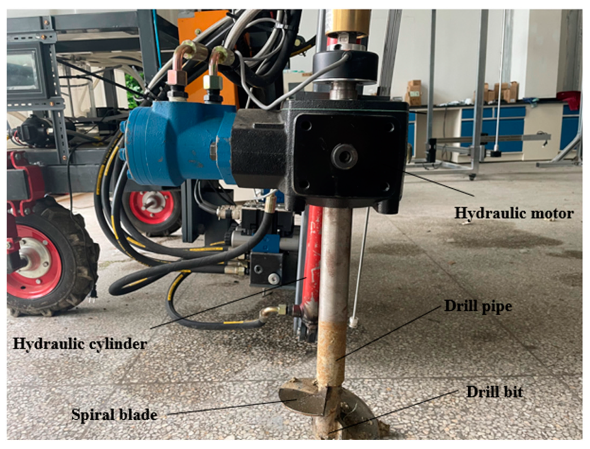
Previous research has calibrated parameters for soil particles in certain regions, providing insights into the impact patterns and predictive models specifically for the vertical resistance of mechanical equipment. However, there is a lack of comparative analysis for the resistance in the other two directions and a comprehensive understanding of the variations in resistance along all three directions. The objective of this study is to precisely calibrate the interaction parameters between cohesive soil in Southern orchards and the borehole fertilization drilling device. Additionally, a simulation analysis of the three-dimensional working resistance of the spiral drilling tool is conducted. The study involves designing the three-dimensional structure of the drilling device using Solid Works and employing the discrete element method software EDEM2021 to build a simulation model for the interaction between soil–soil and soil–drilling-device. Simulation experiments are performed to replicate the drilling process, analyzing the influence of rotational speed and feed rate on torque and resistance. Finally, a simulation analysis is conducted to understand the impact of various experimental factors on the three-dimensional resistance experienced by the spiral drilling tool, aiming to derive a combination of operational parameters with lower energy consumption. This research establishes a soil–soil and soil–spiral-drilling-tool interaction model tailored to the soil conditions prevalent in Southern orchards, enhancing model accuracy by setting the soil particle model radius. The results of the simulation analysis on the three-dimensional working resistance of the spiral drilling tool provide valuable reference data for the analysis of fertilization energy consumption, as well as studies on equipment vibration and wear.

2. Discrete Element Parameter Model and Parameter Calibration of Soil–Soil Interaction

2.1. Soil Basic Parameter

This study utilized soil from the orchard of the Jiangsu Academy of Agricultural Sciences in China. On 17 September 2023, field soil compaction tests were conducted using an SC900 soil compaction meter. The measurements were in kilopascals (kPa) with a resolution of 35 kPa, an accuracy of 103 kPa, and a range of 0–45 cm and 0–7000 kPa. The maximum insertion speed was 25 mm·s⁻¹, and the maximum load was 95.25 kg. The cone head had a circular cone with a diameter of 20 mm and a cone angle of 30° (see Figure 1). The field compaction tests aimed to evaluate soil compaction, which refers to the contact status between soil particles and the size and arrangement of soil pores. This parameter has a significant impact on plant growth and the sustainable use of land. The soil compaction tests were conducted four times, and the specific data are presented in

Table 1. Soil compactness at different depths.

Depth/cm	Pressure/kPa
	1	2	3	4
10	276	586	517	793
20	1207	724	621	828
30	1863	931	1069	862
40	1897	1104	1242	1311

.

According to ASABE (formerly known as the American Society of Agricultural and Biological Engineers) standards, the cone index (CI) is defined as the average pressure per unit area when a standard cone is inserted into the soil at a constant rate. CI serves as a characterization of soil compaction [24]. The formula for calculating CI is expressed as follows:

$$CI=\frac{N}{S}=\frac{F+G}{S}$$

(1)

In the equation, where N represents the pressure at the base of the cone, S is the base area of the cone, F is the external force applied by the operator to the penetrometer, and G is the gravitational force acting on the instrument. This calculation yields a soil compaction of 1.57 g·cm⁻³. The measured average moisture content in the 0–80 mm soil layer is 16.8%. Upon observation, the soil particles are mostly spherical, with few pores, and exhibit a granular shape, which can be simplistically considered as spherical particles.

2.2. Test Method

This study employs a combined approach of physical experiments and simulation experiments [25,26] for calibrating the parameters of a soil discrete element model. Initially, physical experiments were conducted using a universal testing machine to create soil particle piles by lifting a steel plate. The actual pile angle (angle of repose) was measured using an angle measurement device. Subsequently, EDEM2021 software was employed for discrete element simulation experiments. The study began by employing Design Expert 13.0 to perform a Plackett–Burman Design analysis on the parameters of the soil discrete element model, selecting those with significant influence. The most influential parameter values were then determined through a steepest ascent experiment. A regression model for the soil pile angle and significant parameters was established and optimized using the response surface analysis method with the Box–Behnken Design. The resulting regression equation was validated through physical experiments to ensure the accuracy of the simulation parameters.

2.3. Physical Test of Soil Accumulation Angle

The experimental method employed in this study involved the use of a steel plate lift, as illustrated in Figure 2. During the experiment, the steel plate was initially wedged against one side of a cube. Subsequently, soil was poured into the cubic chamber until the latter was completely filled. A universal testing machine was utilized to lift the steel plate upwards at a speed of 0.03 m/s, resulting in the formation of a particle pile, as depicted in Figure 3. Finally, a tilt angle gauge was employed to measure the angle of soil accumulation. The physical experiments for the angle of repose were repeated 10 times, and the average value taken, ultimately yielding an actual soil pile angle of 35.55°.

2.4. Simulation Model

2.4.1. Contact Model

Utilizing an appropriate contact model is a crucial prerequisite for accurately modeling soil in EDEM. The soil samples in this study exhibited macroscopically high adhesion and cohesion characteristics. Therefore, simulation was conducted using the Hertz–Mindlin model with JKR contact model [27]. Due to contact induced by particle motion, the surfaces of the particles gradually deformed during the contact process, resulting in contact forces. The implementation of normal elastic contact force, F_JKR, in this model depends on the overlap distance (δ) and interaction parameters, namely surface energy (γ), defined by the following equation:

$$F_{JKR}=-4\sqrt{\pi \gamma E*}{\alpha }^{\frac{3}{2}}+\frac{4E*}{3R*}{\alpha }^3$$

(2)

$$\delta =\frac{{\alpha }^2}{R*}-\sqrt{\frac{4\pi r\alpha }{E*}}$$

(3)

In the equation, F_JKR represents the JKR normal elastic force, measured in Newtons (N), δ and α denote the overlap distance and radius of the two contacting particles, measured in meters (m), γ represents the surface energy, measured in Newton-meters per square meter (N·m⁻¹), E* is the equivalent elastic modulus, measured in Pascals (Pa), and R* signifies the equivalent radius, also measured in meters (m). The following formula can be employed for the determination:

$$\frac{1}{E*}=\frac{1-v^2}{E_1}+\frac{1-v^2}{E_2}$$

(4)

$$R*=\frac{1}{R_1}-\frac{1}{R_2}$$

(5)

where ν₁ and ν₂ are the Poisson’s ratios of the two particles, E₁ and E₂ represent the shear moduli of the two contacting particles in Pascals (Pa), and R₁ and R₂ denote the radii of the two contacting particles in meters (m).

2.4.2. Soil Particle Model and Particle Factory Establishment

Before conducting simulations, it is necessary to model the soil particle system. Soil is a medium characterized by nonlinearity and discreteness, with a complex interweaving of composition and structure. The spatial configuration information of soil particles cannot be directly obtained. While ensuring the integrity of the soil discrete element model, this paper, for the convenience of simulation experiments, adopts the approach of approximating the geometric morphology of real soil particles using standard spherical particles and combinations of these spheres when modeling soil particles with the discrete element method. This significantly enhances simulation efficiency. To more accurately simulate the geometric morphology of real soil particles in Southern Chinese orchards, single-sphere particles, double-sphere particles, triple-sphere particles, and quadruple-sphere particles were used to model soil particles with different shapes. It is worth noting that a reduction in particle size in discrete element simulations leads to an exponential growth in simulation run time [28]. Considering both computer performance and experimental accuracy, and in line with real soil particles, this study selected a particle radius of 4 mm. Through experimentation and reference to relevant literature [23,29,30], the basic parameters for soil and steel plates were obtained, as presented in

Table 2. Basic parameters of soil and steel plate.

Materials	Poisson’s Ratio	Shear Modulus/Pa	Density/(g·cm−3)
Soil	0.35	1.00 × 106	1.57
Steel plate	0.30	7.94 × 1010	7.85

.

2.4.3. Setting of Simulation Parameters

In EDEM, a cuboid with a side length of 100 mm, a particle factory, and a 100 mm × 100 mm steel plate were established. The lifting speed of the steel plate was set at 30 mm·s⁻¹ (chosen to best reflect the effectiveness of soil particle parameters). A total of 2000 particles were generated at a rate of 1000 particles/s, with a fixed duration equal to 25% of the Rayleigh time step. Data was saved at 0.02 s intervals, and the grid size was set to 2 mm.

2.5. Simulation Test

2.5.1. Plackett–Burman Design Test

Not all parameters in the contact and contact model parameters have a significant impact on the heap angle. Parameters without a significant impact cannot be calibrated based on the heap angle, otherwise the calibrated parameters would be inaccurate. Therefore, based on existing literature research and comprehensive analysis, the range of parameter values to be calibrated was determined. The Plackett–Burman Design module in Design Expert was utilized to select parameters with a significant impact from multiple parameters. Considering the parameters required for EDEM simulation and excluding those directly measurable, such as density, Poisson’s ratio, and elastic modulus of soil particles, seven parameters were selected for calibration, as shown in

Table 3. Virtual calibration discrete element parameter setting table.

Test Parameters	Low Level (−1)	Hight Level (+1)
Soil-particle–soil-particle restitution coefficient A	0.35	0.80
Soil-particle–soil-particle static friction coefficient B	0.36	0.80
Soil-particle–soil-particle rolling friction coefficient C	0.20	0.70
Soil-particle–steel restitution coefficient D	0.20	0.50
Soil-particle–steel static friction coefficient E	0.50	0.80
Soil-particle–steel rolling friction coefficient F	0.05	0.40
Surface energy of soil particle G/J·m−2	3.5	10.5

: soil-particle–soil-particle restitution coefficient (A), soil-particle–soil-particle static friction coefficient (B), soil-particle–soil-particle rolling friction coefficient (C), soil-particle–steel restitution coefficient (D), soil-particle–steel static friction coefficient (E), soil-particle–steel rolling friction coefficient (F), and JKR surface energy (G). According to reference [9], the range of soil particle restitution coefficient is 0.35–0.8, the static friction coefficient is 0.36–0.6, the rolling friction coefficient is 0.2–0.7, the range of restitution coefficient between soil particles and steel is 0.2–0.5, the static friction coefficient is 0.5–0.8, the rolling friction coefficient is 0.05–0.4, and the range of soil JKR surface energy is 3.5–10.5 J·m⁻². In this study, a Plackett–Burman design table with N = 12 was used, with the soil particle heap angle Y as the response value. Each parameter in Table 3 took one high level and one low level, and a total of 12 tests were conducted. The experimental items and results are shown in

Table 4. Scheme and results of Plackett–Burman Design.

No.	Test Parameter							Repose Angle θ/(°)
	A	B	C	D	E	F	G
1	0.80	0.80	0.20	0.20	0.50	0.40	3.50	32.24
2	0.35	0.36	0.20	0.50	0.50	0.40	10.50	41.82
3	0.80	0.36	0.70	0.50	0.80	0.05	3.50	30.09
4	0.35	0.36	0.70	0.20	0.80	0.40	3.50	32.66
5	0.35	0.80	0.70	0.20	0.80	0.40	10.50	40.11
6	0.35	0.36	0.20	0.20	0.50	0.05	3.50	34.38
7	0.35	0.80	0.70	0.50	0.50	0.05	3.50	35.37
8	0.35	0.80	0.20	0.50	0.80	0.05	10.50	40.68
9	0.80	0.36	0.20	0.20	0.80	0.05	10.50	39.67
10	0.80	0.80	0.20	0.50	0.80	0.40	3.50	29.79
11	0.80	0.80	0.70	0.20	0.50	0.05	10.50	37.25
12	0.80	0.36	0.70	0.50	0.50	0.40	10.50	44.69

.

The Design-Expert 13.0 software was used to conduct a significance analysis of the results, leading to the determination of the significance of each simulation parameter, as shown in

Table 5. ANOVA of Plackett–Burman Design test result.

Parameters	Degree of Freedom	Sum of Squares	Mean Square	F-Value	p-Value
A	1	12.59	12.59	19.20	0.0119
B	1	0.0631	0.0631	0.0962	0.7719
C	1	0.0290	0.0290	0.0442	0.8437
D	1	0.0631	0.0631	0.0962	0.7719
E	1	11.51	11.51	17.55	0.0138
F	1	0.8164	0.8164	1.25	0.3270
G	1	197.56	197.56	301.34	<0.0001

. The JKR surface energy coefficient (G) of the soil had a p-value of less than 0.01, signifying an extremely significant impact on the simulated pile angle. The restitution coefficient among soil particles (A) and the static friction coefficient between soil and steel (E) had p-values lower than 0.05, indicating a significant influence on the simulated pile angle. For the remaining simulation parameters, with p-values greater than 0.05, their impact on the simulated pile angle was minimal. As indicated by the Pareto chart in Figure 4, the soil JKR surface energy (G) coefficient exceeds the Bonferroni limit, exerting a highly significant influence on the heap angle. Moreover, both the soil–soil restitution coefficient (A) and the soil–steel static friction coefficient (E) surpass the t-value limit, indicating a significant impact on the heap angle. The analysis revealed that the insignificant impact of the rolling friction coefficient on the heap angle was attributable to the shape of soil particles. Soil particles are non-spherical, and the impact of the soil–steel static friction coefficient on the heap angle was more significant than that of the rolling friction coefficient. The insignificant influence of the soil–soil static friction coefficient was due to the establishment of four soil particle models (single spherical particle, double spherical particle, triple spherical particle, and quadruple spherical particle). The soil–steel restitution coefficient had no significant impact because there was no evident elastic collision between them during the experiment.

2.5.2. The Steepest Climb Test Determined the Optimal Range of Significance Parameters

Based on the experimental results from the previous Plackett–Burman Design, the steepest ascent experiment incrementally increased only the three significant parameters (G, A, E) with a selected step size, while the non-significant parameters (B, C, D, F) were tested at low levels. The relative error between the simulated soil pile angle and the actual pile angle was calculated. The experimental plan and results are presented in

Table 6. Scheme and results of steepest ascent test.

No.	Test Factors			Angle of Accumulation (°)	Relative Error/%
	G	A	E
1	3.50	0.35	0.50	34.38	3.29
2	5.80	0.5	0.60	36.10	1.55
3	8.20	0.65	0.70	37.25	4.78
4	10.5	0.80	0.80	39.67	11.59

.

From Table 6, it can be observed that, as the JKR surface energy (G) of the soil, the restitution coefficient among soil particles (A), and the static friction coefficient between soil and steel (E) increase, the simulated soil particle pile angle steadily increases. The relative error between the simulated pile angle and the actual pile angle initially decreases and then increases. The second set of simulation experiments has the smallest relative error, indicating that the optimal value range for the three significant parameters is near the levels selected in the second set of experiments. Therefore, the levels chosen in the first, second, and third sets of experiments were used for the Box–Behnken Design response surface analysis experiments to find the optimal parameter combination.

2.5.3. Box–Behnken Design Test

Based on the results of the steepest ascent experiment, a Box–Behnken experiment was conducted using Design-Expert to investigate the three significant parameters. The experiments were designed with three factors and three levels within the selected range of the steepest ascent results. The experimental results are shown in

Table 7. Scheme and results of Box–Behnken Design.

No.	Test Parameter			Repose Angle θ/(°)
	G	A	E
1	3.5	0.35	0.6	34.86
2	8.2	0.35	0.6	36.67
3	3.5	0.65	0.6	35.81
4	8.2	0.65	0.6	36.75
5	3.5	0.5	0.5	35.21
6	8.2	0.5	0.5	36.25
7	3.5	0.5	0.7	34.95
8	8.2	0.5	0.7	37.24
9	5.85	0.35	0.5	34.81
10	5.85	0.65	0.5	35.33
11	5.85	0.35	0.7	35.92
12	5.85	0.65	0.7	36.67
13	5.85	0.5	0.6	35.36
14	5.85	0.5	0.6	34.96
15	5.85	0.5	0.6	35.38
16	5.85	0.5	0.6	35.25
17	5.85	0.5	0.6	35.48

.

The experimental results were analyzed using the software Design-Expert, yielding a quadratic regression model as depicted in

Table 8. ANOVA of Box–Behnken Designer quadratic model.

Source of Variance	Mean Sum of Squares	Degree of Freedom	Mean Square	p-Value
Model	8.59	9	0.9549	0.0020
G	4.62	1	4.62	0.0001
A	0.6612	1	0.6612	0.0255
E	1.26	1	1.26	0.0058
GA	0.1892	1	0.1892	0.1740
GE	0.3906	1	0.3906	0.0662
AE	0.0132	1	0.0132	0.7011
G2	0.9833	1	0.9833	0.0107
A2	0.2700	1	0.2700	0.1136
E2	0.0864	1	0.0864	0.3406
Residual	0.5786	7	0.0827
Lack of Fit	0.4190	3	0.1397	0.1287
Pure Error	0.1595	4	0.0399
Cor Total	9.17	16

. From the table, it is evident that the surface energy (G) and the soil–steel static friction coefficient (E) have a highly significant impact on the soil heap angle (p < 0.01). The regression model itself has a significance level of p < 0.01, indicating an extremely significant relationship between the heap angle and the regression equation obtained. Furthermore, the lack-of-fit term has a p-value of 0.1287, which is greater than 0.05, suggesting that the proportion of abnormal errors in the actual fit of the regression equation is small, indicating a good fit. The coefficient of variation (CV) for this experiment is 0.81%, indicating good reliability. The predictive coefficient R²_pre is 0.8419, the coefficient of determination R² is 0.9369, and the adjusted coefficient of determination R²_adj is 0.8558. This suggests that 85.58% of the variation in response values comes from the selected factors, with a difference of less than 0.2 between the predictive and determination coefficients. The adequacy precision (Adeq Precision) is 11.905, typically desired to be greater than 4, indicating good precision of the regression model. The regression equation is as follows.

$$\begin{array}{l}Angle=\\ 35.29+0.76G+0.2875A+0.3975E\\ -0.2175GA+0.3125GE+0.0575AE\\ +0.4833G^2+0.2533A^2+0.1433E^2\end{array}$$

(6)

By plotting perturbation diagrams based on the existing quadratic polynomial model, as shown in Figure 5, it can be observed that, with the increase in levels of B:A and C:E, there is a gradual increase in the heap angle. The relationship between A:G and the heap angle exhibits a trend of slow increase followed by rapid increase.

Table 8 reveals that, when considering pairwise interactions among the three significant factors, the influence on the heap angle decreases in the following order: GE, GA, and then AE. A detailed analysis of the interaction response surfaces is presented in Figure 6a,c,e. From Figure 6a, it can be observed that, when the soil–steel static friction coefficient (E) remains constant, the heap angle initially decreases and then increases with an increase in the soil JKR surface energy (G), and this change trend is very apparent. When the soil JKR surface energy (G) remains constant, the heap angle also initially decreases and then increases with an increase in the soil–steel static friction coefficient (E), albeit with a slightly diminished change trend compared to the variation in soil JKR surface energy (G). From Figure 6c,e, it can be observed that when one factor remains constant at a certain level, the other factor exhibits a slow increasing trend.

Contour plots are curves formed on the base surface by identical factor values on the surface (Figure 6b,d,f). The closer the contour profile is to a perfect circle, the smaller the interaction between the two factors. Conversely, the closer the contour profile is to an ellipse, the greater the interaction between the factors. In the instance of an interaction, one factor exerts different effects at different levels on another factor.

Using the optimization module within Design-Expert software and setting the measured pile angle value of 35.55° as the target, a close set of solutions was obtained, consisting of the following parameters: JKR surface energy of the soil (G) = 5.85 J·m⁻², restitution coefficient among soil particles (A) = 0.65, and static friction coefficient between soil and steel (E) = 0.5.

2.5.4. Simulation Verification

The quadratic polynomial equation established based on relative error aims to minimize relative error as the target value for solving. The regression model is optimized using the optimization feature in the Design-Expert software, resulting in a unique optimization solution as shown in

Table 9. Optimal relative error solutions.

A	E	G
0.50	0.60	5.80

.

Utilizing the optimization module in the Design-Expert software with the measured pile angle of 35.55° as the target value, a set of closely matching solutions was obtained. The resulting parameters are as follows: soil JKR surface energy G = 5.85 J·m⁻², soil–soil restitution coefficient A = 0.5, and soil–steel static friction coefficient E = 0.6. To validate the reliability of these parameters, three sets of simulation experiments were conducted using the aforementioned parameter combination. The average simulated pile angle was determined to be 35.91°, with a relative error of only 0.01% compared to the measured value. This indicates that the set of parameters exhibits high accuracy and reliability.

To verify the reliability of this parameter set, three sets of simulation experiments were conducted using the aforementioned combination as simulation parameters. The average simulated pile angle was determined to be 35.91°, with a relative error of only 0.01% compared to the measured value. This indicates that the parameter set exhibits high accuracy and reliability. The comparison between simulation and physical experiments is illustrated in Figure 7.

3. Discrete Element Model for the Interaction between Drilling Device and Soil

3.1. Establishment of Simulation Model

The model of the designed drilling device was created using Solidworks, a three-dimensional drafting software. The model was saved in the .stl file format and imported into EDEM, as shown in Figure 8. The dimensions of the soil slot were determined to be a diameter of 200 mm and a height of 600 mm, based on the actual needs of the pit diameter and depth. The parameter settings were chosen according to the basic parameters determined earlier, as indicated in

Table 10. Basic parameters of simulation model.

Basic Parameter	Numerical Value
Soil-particle–soil-particle restitution coefficient	0.65
Soil-particle–soil-particle static friction coefficient	0.36
Soil-particle–soil-particle rolling friction coefficient	0.2
Soil-particle–steel restitution coefficient	0.2
Soil-particle–steel static friction coefficient	0.5
Soil-particle–steel rolling friction coefficient	0.05
Surface energy of soil particle/J·m−2	5.85

. The contact model for soil particles and the helical drill rod utilized the Hertz–Mindlin non-sliding contact model. A total of 140,000 particles were generated, with 28,000 particles generated per second. The drilling device began its downward drilling movement in the simulation at 5 s, and the total simulation time was set to 10 s.

To validate the accuracy of the EDEM simulation model, comparative experiments were conducted using a custom-built prototype at the Jiangsu Academy of Agricultural Sciences, as depicted in Figure 9.

3.2. Analysis of Simulation Results of Different Speed and Feed Speed

3.2.1. Comparative Analysis of Torque at Different Speed

The simulation model was configured with a maximum soil penetration depth of 80 mm for the drilling device, a linear feed rate of 0.05 m/s for the auger, and a data-saving interval of 0.02 s. Four sets of simulation experiments were conducted. In the data analysis module, experimental result data were exported, focusing on the data recorded between 5 s to 10 s. The variation pattern of the torque experienced by the auger during drilling is illustrated in Figure 10.

As observed in Figure 10, the variation trends of the torque experienced by the drill shaft in the four experimental sets are essentially consistent. In each case, the torque initially increases from zero to a maximum value, then gradually decreases to a lower level, followed by a repetition of the earlier trend. This alignment corresponds to the contact status between the drilling device and the soil during the drilling process. The helical drilling process can be roughly divided into four stages. In the first stage, before the drill bit penetrates the soil, the torque is nearly zero. As the drill bit drives the helical shaft to longitudinally cut into the soil, the volume of cut soil gradually increases, leading to an increase in torque. Subsequently, the helical blades enter a lateral cutting state, interacting with the soil, causing a sudden increase in torque. With the rotation of the blades, when the first layer of helical blades is fully embedded in the soil, the torque reaches its maximum value. In the second stage, as the first layer of helical blades continues to drill downward, the contact area increases, resulting in a corresponding decrease in torque. In the third stage, when the torque decreases to a certain low value, the next layer of helical blades begins to enter the drilling state. Both the front and rear layers of the blades simultaneously drill into the soil, causing a rapid increase in torque. In the fourth stage, as the contact area between the drill rod and the soil gradually increases, the torque gradually decreases again. This process repeats in a cyclic manner.

Analyzing the maximum torque values from Figure 10a–d reveals that, as the blade rotation speed increases, the required power consumption for drilling operations also increases. Simultaneously, with higher rotation speeds, the drilling frequency per unit time increases, leading to a shorter interval between peak values, aligning well with practical expectations. Comparing the simulation results with the soil trench experiment results, as shown in Figure 11, the trends in simulated and experimental values are consistent. Torque increases with higher rotation speeds, and the maximum relative error is 7%. The simulation results effectively capture the variation patterns in drilling power consumption and accurately represent torque values. Hence, using the EDEM simulation model developed in this study to assess the working resistance experienced by the spiral blades is reliable. The experimental values for soil tend to be slightly higher than the simulated values, possibly due to additional power consumption caused by environmental factors such as stones in the soil.

3.2.2. Comparative Analysis of Total Force at Different Feed Speeds

The simulation model was configured with a maximum soil penetration depth of 80 mm for the drilling device, a helical rotation speed of 200 r·min⁻¹ for the auger, and a data-saving interval of 0.02 s. Three sets of simulation experiments were conducted. In the data analysis module, experimental result data were exported, focusing on the data recorded between 5 s to 10 s. The variation pattern of the total force experienced by the auger during drilling is illustrated in Figure 12.

As depicted in Figure 12, the variation trends of the total force experienced by the drilling devices at three different feed rates are roughly similar. At 0.03 m/s, the total force abruptly increases after 6.5 s, gradually rising to a peak of 408 N. Subsequently, it fluctuates within a range of approximately 250 N. At 0.05 m/s, the total force sharply increases at 6 s, reaching a maximum value of 301 N, and then fluctuates within a range of around 200 N. For a feed rate of 0.07 m/s, the total force begins to sharply increase after 5.5 s, reaching a maximum value of 327 N, and subsequently fluctuates within a range of approximately 225 N.

3.2.3. Analysis of Three-Way Working Resistance

• Force analysis

As illustrated in Figure 13, selecting the spiral blades as the objects for force analysis, the directions of the three-dimensional working resistances are defined as follows: along the rotation direction of the spiral main axis is the positive horizontal resistance (F_x), downward from the soil surface is the positive vertical resistance (F_y), and inward from the vertical blade is the positive lateral resistance (F_z).

2.

The influence of speed on three-way resistance

With a fixed tillage depth of 80 mm, a feed rate of 0.05 m/s, and rotational speeds of 100 r·min⁻¹, 200 r·min⁻¹, 300 r·min⁻¹, and 400 r·min⁻¹, four sets of simulation experiments were conducted. The variation in the maximum three-dimensional resistances experienced by the spiral blades with respect to rotational speed is depicted in Figure 14. The maximum resistance encountered by the spiral blades in the vertical direction surpasses that encountered in the horizontal and lateral directions, with vertical resistance being the primary factor influencing drilling power consumption. The maximum values of horizontal and lateral resistances are roughly similar. As the rotational speed increases, the maximum vertical resistance continues to rise, while horizontal and lateral resistances show a declining trend. When the speed exceeds 200 r·min⁻¹, the decline in horizontal and lateral resistances becomes gradual. However, when the speed exceeds 300 r·min⁻¹, both resistances in these directions experience a sudden increase. This phenomenon is attributed to the surrounding soil resisting the downward rotational motion of the spiral blades during drilling operations, exerting compressive forces on the blades. As the speed increases, the compressive force also intensifies, offsetting some of the forces in the horizontal and lateral directions, resulting in a decreasing trend for these two forces. Simultaneously, with higher speeds, the drilling volume of the spiral blades per unit time increases, leading to a greater force in the vertical direction. However, the relative change in the resultant force on the spiral blades is not significant. The variations in vertical and lateral resistances directly impact the torque experienced by the spiral blades. Soil trench experiments indicate that the torque on the spiral blades also increases with higher rotational speeds, and when the speed exceeds 300 r·min⁻¹ the torque increases more rapidly.

3.

Influence of feed speed on three-directional resistance

With a fixed tillage depth of 80 mm, a rotational speed of 200 r·min⁻¹, and feed rates of 0.03 m/s, 0.05 m/s, and 0.07 m/s, three sets of simulation experiments were conducted. The variation in the maximum three-dimensional resistances experienced by the spiral blades with respect to the feed rate is depicted in Figure 15. Vertical resistance is the primary factor influencing drilling power consumption, and the maximum lateral resistance is slightly greater than the maximum parallel resistance. As the feed rate increases, the maximum resistances in all three directions also increase. When the feed rate exceeds 0.05 m/s, the maximum lateral resistance sharply increases, while the growth rates of the maximum vertical and horizontal resistances remain relatively constant. Soil trench experiments indicate that the torque on the spiral blades increases with faster feed rates, albeit at a relatively moderate rate.

4.

Optimal analysis of variance test

Simulation optimization parameters include rotational speed and feed rate. The rotational speed (n) was varied from 100 r·min⁻¹ to 400 r·min⁻¹, and the feed rate (v) was varied from 0.03 to 0.07 m/s. These factors are considered in a two-factor one-way analysis of variance (ANOVA) experiment with the maximum working torque (M) of the spiral earth auger as the evaluation criterion. The experimental design is outlined in

Table 11. Experimental design and results.

No.	n/(r·min−1)	v/(m/s)	M/(N·m)
1	200	0.05	39.4
2	300	0.03	53.2
3	400	0.05	94.5
4	400	0.07	102.6
5	400	0.03	82.7
6	200	0.05	39.4
7	300	0.05	43.8
8	200	0.03	56.4
9	200	0.07	54.6
10	100	0.05	30.9
11	300	0.05	41.5
12	200	0.03	53.8
13	100	0.03	36.1
14	100	0.03	33.7
15	100	0.05	30
16	300	0.07	61.3
17	100	0.07	50.7

.

As indicated in

Table 12. Analysis of variance.

Source of Variance	Mean Sum of Squares	Degree of Freedom	Mean Square	F-Value	p-Value
Model	7405.73	11	673.25	361.57	<0.0001
n	5894.95	3	1964.98	1055.31	<0.0001
v	701.73	2	350.86	188.43	<0.0001
n v	313.96	6	52.33	28.10	0.0011
Pure Error	9.31	5	1.86
Cor Total	7415.04	16

, both factors have a highly significant impact on power consumption, and the interaction effect is also considerable. Based on the above analysis, it is concluded that the power consumption is optimal when the rotational speed is 100 r·min⁻¹ and the feed rate is 0.05 m/s. Considering M = 30 N·m and n = 100 r·min⁻¹, these values are substituted into the formula:

$$P=\frac{Mn}{9550}$$

(7)

The resulting P is 0.314 kW.

4. Summary and Conclusions

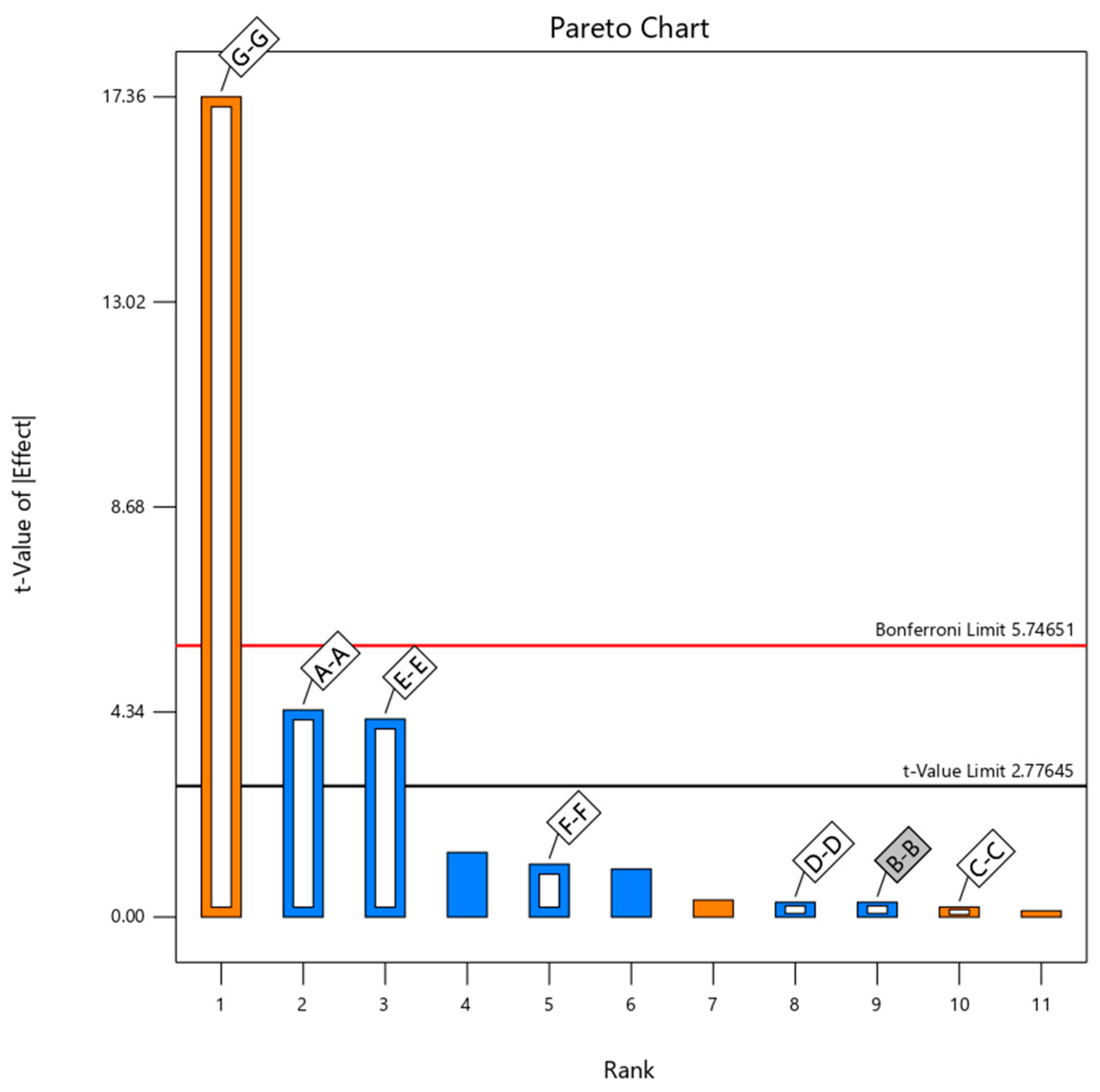
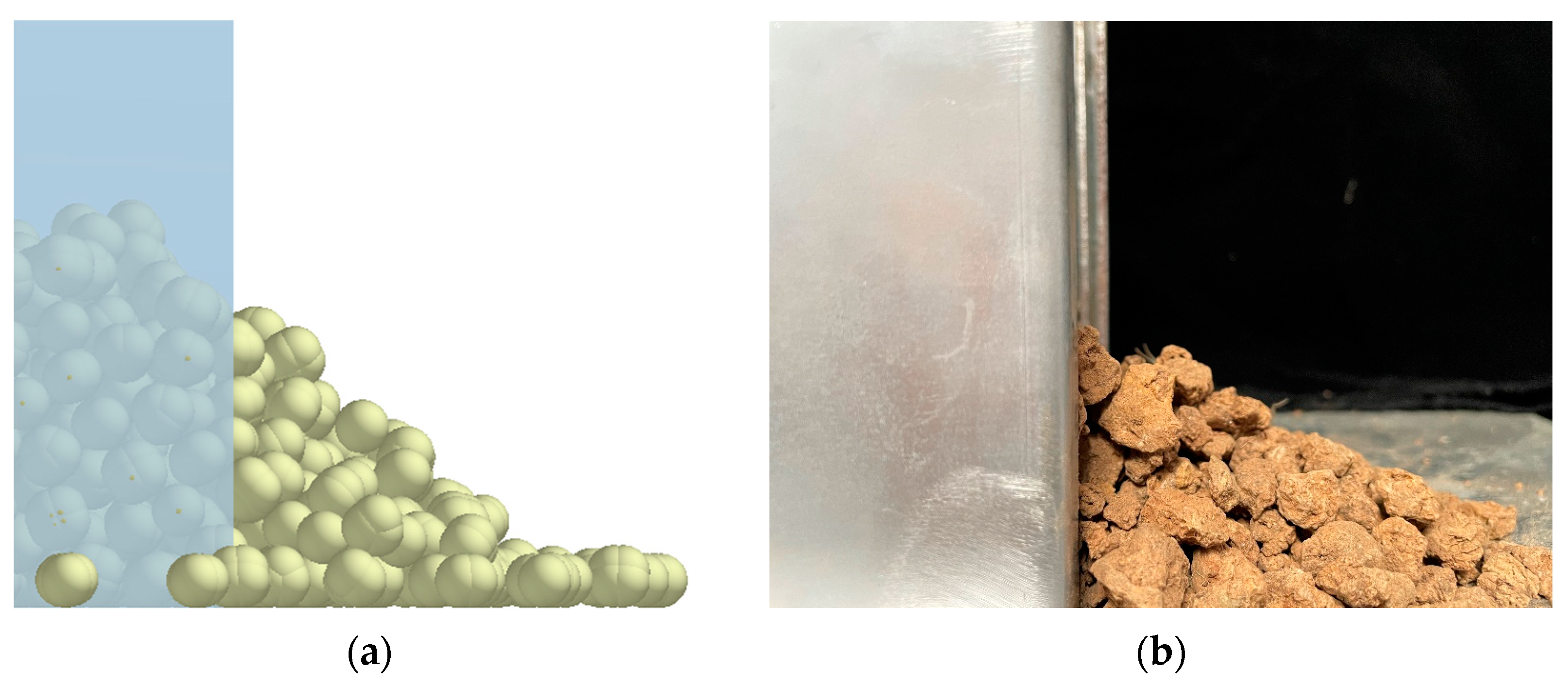
• The particle parameters of southern orchard soil were experimentally measured, and modeling was conducted using the EDEM2021 discrete element software. The Hertz–Mindlin with the Johnson–Kendall–Roberts contact model was employed. Utilizing the Plackett–Burman Design, significant contact parameters and model parameters influencing the soil pile angle were selected. These parameters include soil JKR surface energy, soil–soil restitution coefficient, and soil–steel static friction coefficient.
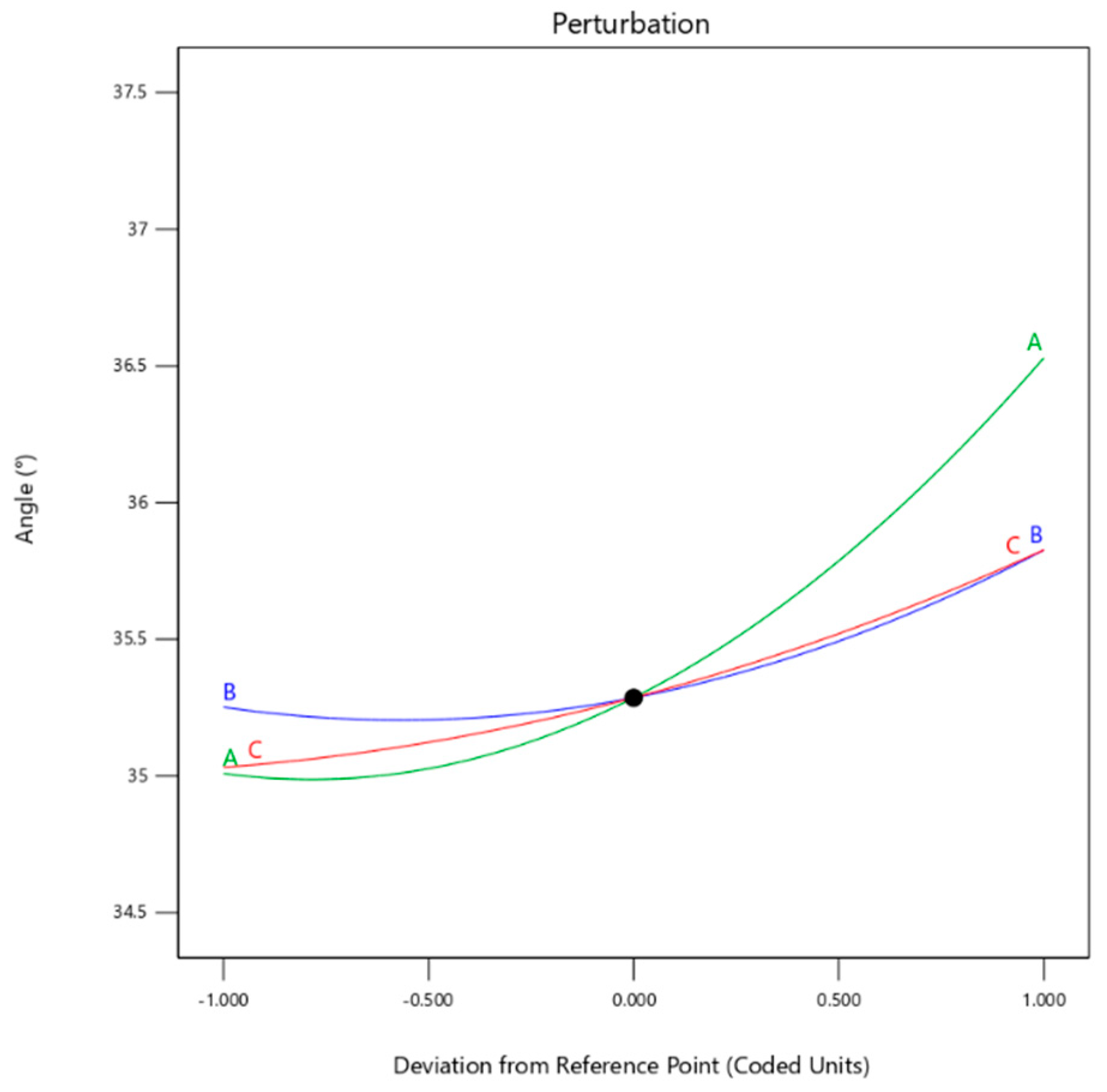
• The optimal value ranges for significant parameters were determined through steepest ascent experiments. Subsequently, a regression model for the soil pile angle and significant parameters was established and optimized using the Box–Behnken Design. The optimal values for the parameters were found to be 5.85 J·m⁻² for the soil JKR surface energy, 0.65 for the soil–soil restitution coefficient, and 0.5 for the soil–steel static friction coefficient. Simulation experiments were conducted under these calibrated parameters, and the relative error between simulated and measured pile angles was determined to be 0.01%.
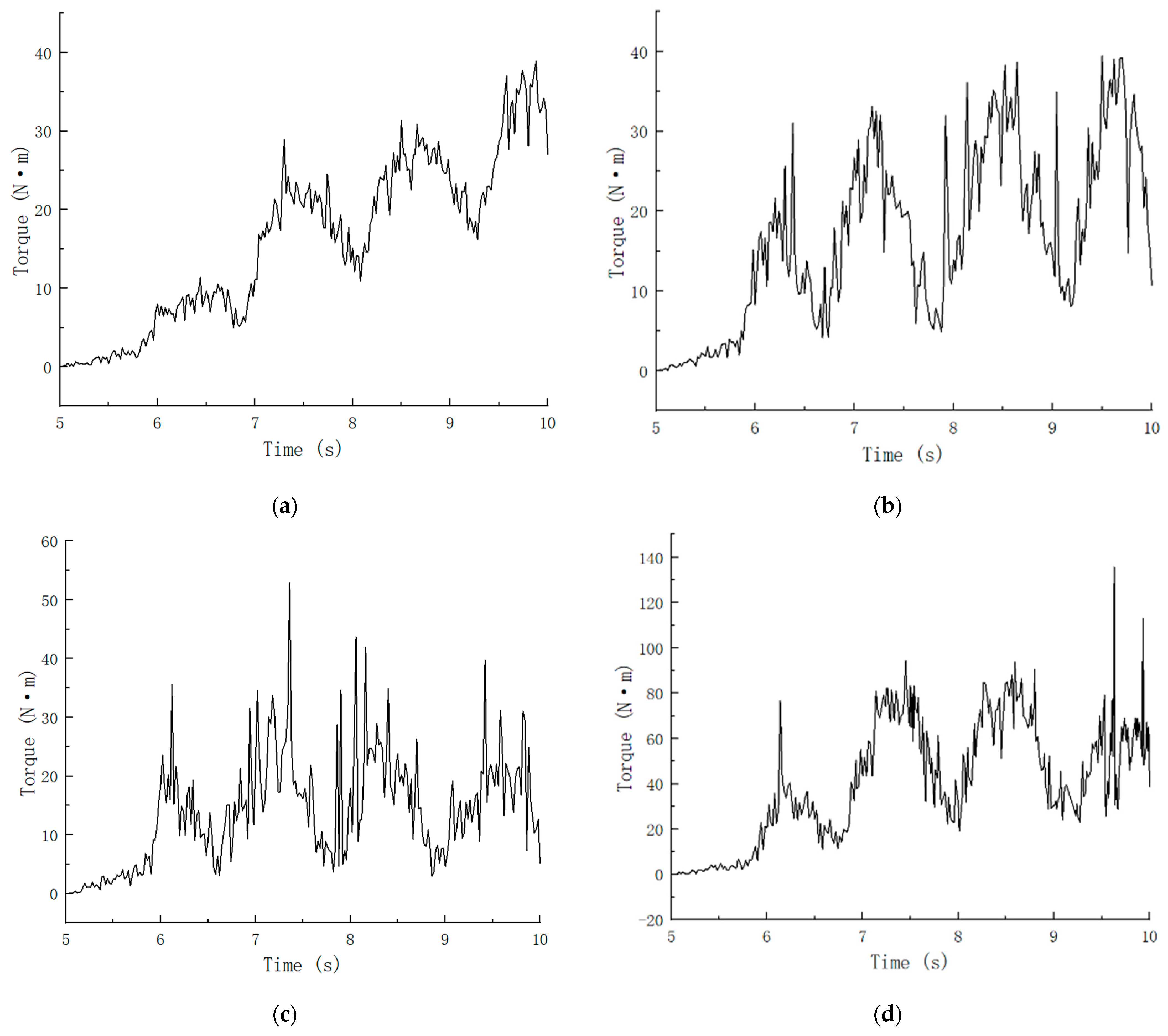
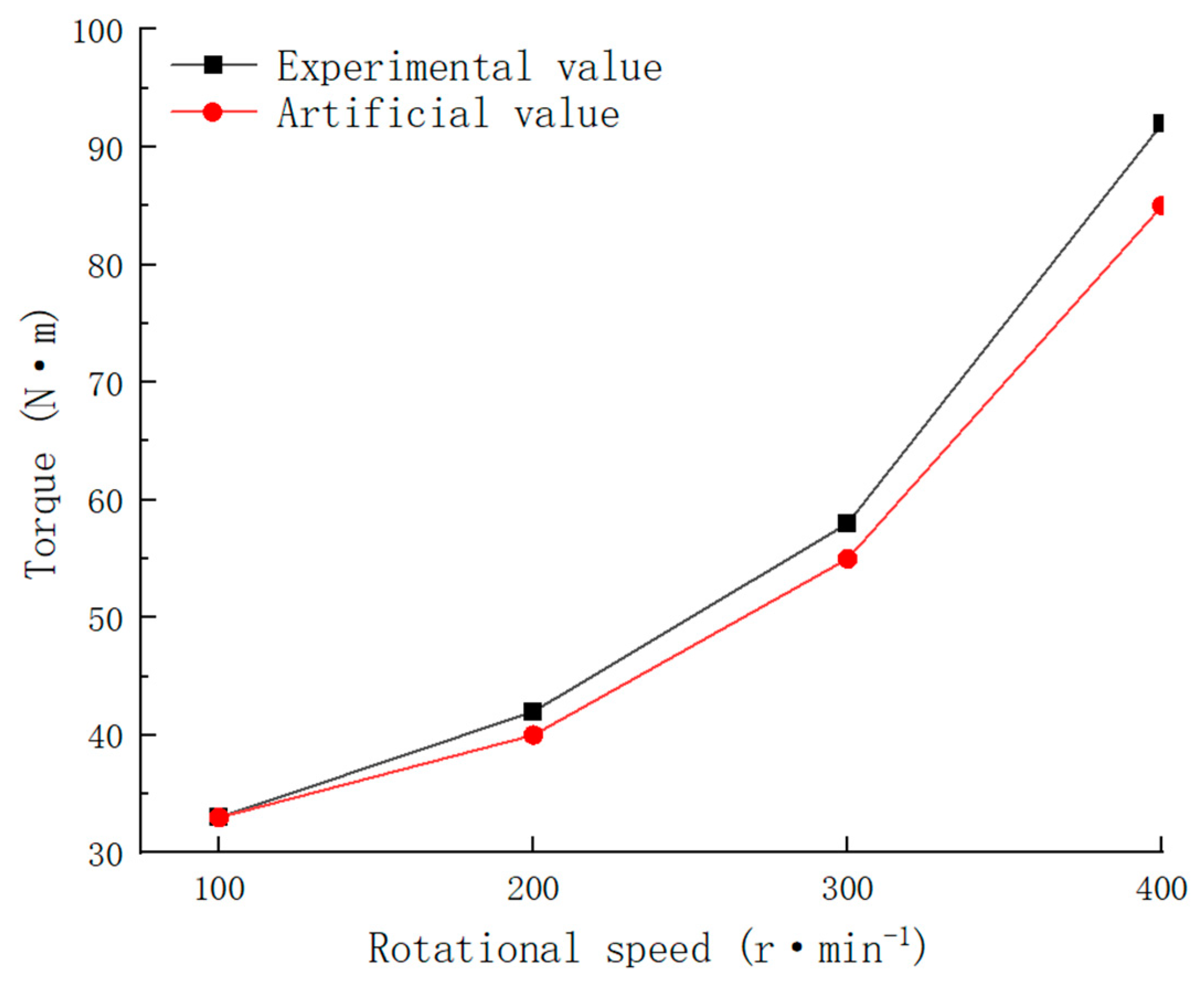
• Torque comparative experiments for spiral earth auger were conducted in a soil trench, and the results indicate that the trends in simulated and experimental values align. The torque increased with higher rotational speeds, with a maximum relative error of 7%. The torque initially rose from 0 to a maximum value, then gradually decreased to a lower value, followed by a rapid increase to a higher value before declining again, repeating this pattern. The average total force at a feed rate of 0.05 m/s was found to be a minimum of 200 N. The simulation model effectively captures the variation patterns in drilling power consumption and accurately represents torque values, demonstrating a certain level of reliability.
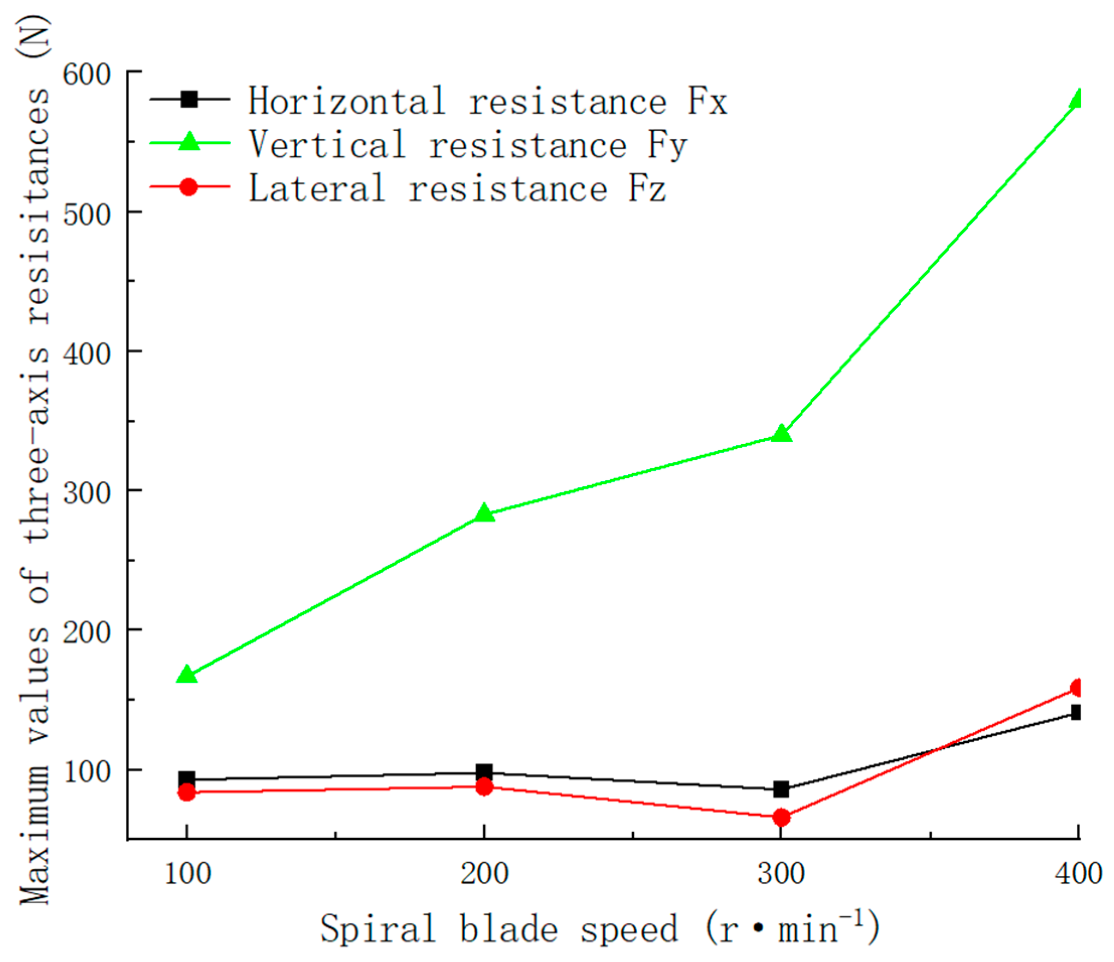
• Among the three forces, vertical resistance is the primary factor contributing to power consumption. As the rotational speed increased, the maximum value of vertical resistance was found to continue to rise, while horizontal and lateral resistances exhibited a declining trend. With an increase in feed rate, the maximum values of resistance in all three directions also increased. When the feed rate exceeded 0.05 m/s, there was a sharp increase in the maximum lateral resistance.
• By analyzing the three-dimensional forces acting on the spiral blades and conducting a comparative analysis at different rotational speeds and feed rates, along with the results from optimal variance analysis experiments, the optimal rotational speed and feed rate were determined to be 100 r·min⁻¹ and 0.05 m/s, respectively. According to the formula, the optimal power consumption is 0.314 kW.

This study demonstrates the accuracy of the Discrete Element Method in analyzing the three-dimensional working resistance of helical cutting tools. The relevant experimental data can serve as a reference for the analysis of equipment energy consumption, machine vibration, and blade wear studies. However, soil is a complex composite with many influencing factors, and accurately describing the contact state of soil particles remains challenging. In order to enhance computational performance, many scholars set the simulated soil particle radius to 5 mm or larger, which is much larger than the actual field soil particle radius. This leads to distorted simulation results. However, if the soil particle radius is divided too finely, the number of simulated soil particles within the soil trough increases geometrically, causing a significant delay in both computation time and efficiency. To set the soil particle radius close to real values while balancing computational load and simulation effectiveness, this paper employs the sieve analysis method to measure the soil particle size range as the basis for determining the simulated soil particle radius. This approach enhances the accuracy of the soil model. However, since the simulated model assumes that single spherical particles, double spherical particles, triple spherical particles, and quadruple spherical particles all have equal diameters, there remains some disparity with the true composition of soil. In subsequent stages, the study will focus on the expression methods of soil properties, such as porosity, uneven-sized particles, and layered compaction in the Discrete Element Model (DEM) to further improve simulation accuracy.

References

1. Xing, J.J.; Zhang, R.; Wu, P. Parameter calibration of discrete element simulation model for lateritic soil particles in Hainan hot area. Trans. Chin. Soc. Agric. Eng. 2020, 36, 158–166. [Google Scholar]
2. Ucgul, M.; Fielke, J.M.; Saunders, C. 3D DEM tillage simulation: Validation of a hysteretic spring (plastic) contact model for a sweep tool operating in a cohesionless soil. Soil Tillage Res. 2014, 144, 220–227. [Google Scholar] [CrossRef]
3. Cundall, P.A.; Strack, O.D. A discrete numerical model for granular assemblies. Geotechnique 1979, 29, 47–65. [Google Scholar] [CrossRef]
4. Fang, H.M.; Ji, C.Y.; Ahmed, A.T. Simulation analysis of straw displacement in straw-soil-rotary tillage tool system. Trans. Agric. Mach. 2016, 1, 60–67. [Google Scholar]
5. Mak, J.; Chen, Y.; Sadek, M.A. Determining parameters of a discrete element model for soil-tool interaction. Soil Tillage Res. 2012, 118, 117–122. [Google Scholar] [CrossRef]
6. Chen, Y.; Munkholm, L.J.; Nyord, T. A discrete element model for soil-sweep interaction in three different soils. Soil Tillage Res. 2013, 126, 34–41. [Google Scholar] [CrossRef]
7. Zhang, R.; Han, D.L.; Ji, Q.L.; He, Y.; Li, J.Q. Research on calibration method of sand and soil parameters in discrete element simulation. Trans. Chin. Soc. Agric. Mach. 2017, 48, 49–56. [Google Scholar]
8. Wang, X.L.; Zhong, X.K.; Geng, Y.L.; Wei, Z.C.; Hu, H.; Geng, D.Y.; Zhang, X.C. Parameter calibration of no-tillage soil based on discrete element nonlinear elastoplastic contact model. Trans. Chin. Soc. Agric. Eng. 2021, 37, 100–107. [Google Scholar]
9. Wu, T.; Huang, W.F.; Chen, X.S.; Ma, X.; Han, Z.Q.; Pan, T. Parameter calibration of discrete element model of viscous soil considering interparticle bonding force. J. South China Agric. Univ. 2017, 38, 93–98. [Google Scholar]
10. He, Y.M.; Xiang, W.; Wu, M.L.; Quan, W.; Chen, C.P. Calibration of discrete element parameters of loam based on accumulation test. J. Hunan Agric. Univ. 2018, 44, 216–220. [Google Scholar]
11. Li, J.W.; Tong, J.; Hu, B.; Wang, H.B.; Mao, C.Y.; Ma, Y.H. Discrete element simulation parameter calibration of interaction between viscous black soil with different moisture content and earth-touching components. Trans. Chin. Soc. Agric. Eng. 2019, 35, 130–140. [Google Scholar]
12. Koushkaki, R.H.; Eshkaftaki, M.M.; Anejadian, A.H. Simulation of draught force during chisel ploughing using discrete element method. J. Biosyst. Eng. 2022, 47, 152–166. [Google Scholar] [CrossRef]
13. Zeng, Z.; Ma, X.; Chen, Y. Modelling residue incorporation of selected chisel ploughing tools using the discrete element method (DEM). Soil Tillage Res. 2020, 197, 104505. [Google Scholar] [CrossRef]
14. Ding, Q.S.; Ren, J.; Belal, E.A.; Zhao, J.K.; Ge, S.Y.; Li, Y. Discrete element analysis of subsoiling process in wet clay paddy soil. Trans. Chin. Soc. Agric. Mach. 2017, 48, 38–48. [Google Scholar]
15. Sun, J.B.; Liu, Q.; Yang, F.Z.; Liu, Z.J.; Wang, Z. Discrete element simulation parameter calibration for interaction between slope soil and rotary tillage components in Loess Plateau. Trans. Chin. Soc. Agric. Mach. 2022, 53, 63–73. [Google Scholar]
16. Shi, L.R.; Zhao, W.Y.; Sun, W. Soil particle contact model and parameter calibration in northwest arid region based on discrete elements. Trans. Chin. Soc. Agric. Eng. 2017, 33, 181–187. [Google Scholar]
17. Roul, A.; Raheman, H.; Pansare, M. Predicting the draught requirement of tillage implements in sandy clay loam soil using an artificial neural network. Biosyst. Eng. 2009, 104, 476–485. [Google Scholar] [CrossRef]
18. Ahmadi, I. A torque calculator for rotary tiller using the laws of classical mechanics. Soil Tillage Res. 2017, 165, 137–143. [Google Scholar] [CrossRef]
19. Chertkiattipol, S.; Niyamapa, T. Variations of torque and specific tilling energy for different rotary blades. Int. Agric. Eng. J. 2010, 19, 1–14. [Google Scholar]
20. Wang, Z.H.; Huang, D.Y.; Li, Z.S. Universal the blade the broken stubble power consumption influence of the working parameters of the rotary tiller broken stubble. J. Jilin Univ. Eng. Technol. Ed. 2012, 42 (Suppl. S1), 122–125. [Google Scholar]
21. Jiang, J.D.; Gao, J.; Zhao, Y.D. Finite element simulation and analysis on soil rotary tillage with external vibration excitation. Trans. Chin. Soc. Agric. Mach. 2012, 43, 58–62. [Google Scholar]
22. Fang, H.M. Study on Mechanism of Straw-Soil-Rotary Blade Interaction Based on Discrete Element Method; Nanjing Agricultural University: Nanjing, China, 2016. [Google Scholar]
23. Xion, P.Y.; Yang, Z.; Sun, Z.Q.; Zhang, Q.Q.; Huang, Y.Q.; Zhang, Z.W. Simulation analysis and test of three-way working resistance of rotary tillage cutter based on discrete element method. Trans. Chin. Soc. Agric. Eng. 2018, 34, 113–121. [Google Scholar]
24. Tian, H.; Gao, C.; Zhao, Y. Combined penetrometer and standing wave ratio probe to measure compactness and moisture content of soils. Appl. Ecol. Environ. Res. 2019, 17, 6. [Google Scholar] [CrossRef]
25. Rackl, M.; Hanley, K.J. A methodical calibration procedure for discrete element models. Powder Technol. 2017, 307, 73–83. [Google Scholar] [CrossRef]
26. Coetzee, C.J. Calibration of the discrete element method. Powder Technol. 2017, 310, 104–142. [Google Scholar] [CrossRef]
27. Du, J.; Heng, Y.; Zheng, K. Investigation of the burial and mixing performance of a rotary tiller using discrete element method. Soil Tillage Res. 2022, 220, 105349. [Google Scholar] [CrossRef]
28. Fang, H.M.; Ji, C.Y.; Farman, A.C.; Guo, J.; Zhang, Q.Y. Analysis of soil movement behavior during rotary tillage based on discrete element method. Trans. Chin. Soc. Agric. Mach. 2016, 47, 22–28. [Google Scholar]
29. Wang, X.L.; Hu, H.; Wang, Q.J.; Li, H.W.; He, J.; Chen, W.Z. Parameter calibration method of soil model based on discrete element. Trans. Chin. Soc. Agric. Mach. 2017, 48, 78–85. [Google Scholar]
30. Yuan, Q.C.; Xu, L.M.; Xing, J.J.; Duan, Z.Z.; Ma, S.; Yu, C.C. Parameter calibration of discrete element model of organic fertilizer particles applied by machine. Trans. Chin. Soc. Agric. Eng. 2018, 34, 21–27. [Google Scholar]
Figure 1. SC900 soil compactness meter.
Applsci 14 02642 g001
Figure 2. Physical test of soil accumulation Angle.
Applsci 14 02642 g002
Figure 3. Soil particle pile.
Applsci 14 02642 g003
Figure 4. Pareto chart of Plackett–Burman Design.
Applsci 14 02642 g004
Figure 5. Perturbation diagram.
Applsci 14 02642 g005
Figure 6. GE interaction analysis diagram of response surface. (a) GE Response surface, (b) GE Contour line, (c) AG Response surface, (d) AG Contour line, (e) AE Response surface, (f) AE Contour line.
Applsci 14 02642 g006
Figure 7. Comparison of simulation and physical tests. (a) Simulation test, (b) Physical test.
Applsci 14 02642 g007
Figure 8. Simulation model of EDEM.
Applsci 14 02642 g008
Figure 9. Prototype.
Applsci 14 02642 g009
Figure 10. The torque change of the drilling shaft under different speed. (a) 100 r·min−1, (b) 200 r·min−1, (c) 300 r·min−1, (d) 400 r·min−1.
Applsci 14 02642 g010
Figure 11. Comparison of simulation and test results of torque at different speed.
Applsci 14 02642 g011
Figure 12. The total force change of drilling shaft with different feed speed. (a) 0.03 m/s, (b) 0.05 m/s, (c) 0.07 m/s.
Applsci 14 02642 g012
Figure 13. Direction of three-axis working resistance. Note: Fx is the horizontal resistance, Fy is the vertical resistance under the vertical soil face, Fz is the inward lateral resistance of the vertical spiral blade, N, v is the downward feed speed of the tool, m/s, n is the rotational speed of the spiral blade, r·min−1.
Applsci 14 02642 g013
Figure 14. The change of the maximum triaxial resistance with the rotation speed of the spiral blade.
Applsci 14 02642 g014
Figure 15. The change of the maximum triaxial resistance with the feed speed.
Applsci 14 02642 g015