A Tube Linear Model Predictive Control Approach for Autonomous Vehicles Subjected to Disturbances

Abstract

The path tracking performance of autonomous vehicles is degraded by common disturbances, especially those that affect the safety of autonomous vehicles (AVs) in obstacle avoidance conditions. To improve autonomous vehicle tracking performances and their computational efficiency when subjected to common disturbances, this paper proposes a tube linear model predictive controller (MPC) framework for autonomous vehicles. A bicycle vehicle dynamics model is developed and employed in the tube MPC control design in the proposed framework. A robust invariant set is calculated with an efficient linear programming (LP) method, and it is used to guarantee that the constraints are satisfied under common disturbance conditions. The results show that the computational cost of robust positively invariant sets that are constructed by the LP method is much less than that obtained by the traditional method. In addition, all the trajectories of the tube linear MPC successfully avoided obstacles when under disturbance conditions, but only about 80% of the trajectories obtained with the traditional MPC successfully avoided obstacles under disturbance conditions. The proposed framework is effective.

1. Introduction

With the increase in the number of vehicles, traffic safety and efficiency have become a severe issue for governments and humans [1,2,3,4,5]. Autonomous vehicles can provide more excellent safety benefits and improve traffic efficiency, and they are assumed to be an efficient solution for traffic safety and efficiency issues [6,7,8]. The control layer for automatic vehicles has a significant effect on traffic safety and efficiency issues, and many scholars have devoted themselves to creating effective control methods for automatic vehicles [9,10,11,12].

The commonly used controllers are LQR (Linear Quadratic Regulator) [13], fuzzy logic control [14], sliding mode control [15], and backstepping [16,17]. Compared with other controllers, model predictive control has better real-time performance, stability, and robustness [13]. Therefore, it is widely used in AVs. Li et al. [18] designed a non-linear MPC controller that navigates AVs to avoid obstacles. The non-linear MPC method introduces a computational burden during the iterative calculations of MPC and requires expensive hardware configurations, which makes the non-linear MPC difficult to apply in practical engineering applications. To deal with the issue, many scholars [19,20,21] have carried out a great deal of studies. Li et al. [22] proposed a lower-dimensional MPC approach that entailed a trade-off between the tracking performance and the computational burden. Hoffmann et al. [23] employed the linear time-varying (LTV) approach to decrease the online computational burden of the MPC. However, the tracking performance is degraded under disturbance conditions, like parameter uncertainty and cross-wind [24]. For example, due to the cross-wind disturbance, the actual path of a vehicle deviates from its planned path and the vehicle impacts with the obstacle (see Figure 1).

To attenuate the disturbances in the MPC, Mayne et al. [25] proposed a tube non-linear MPC approach to ensure that the states satisfy the constraints when under common disturbance conditions. Gao et al. [26] adopted a tube non-linear MPC for lane keeping and obstacle avoidance when under disturbance conditions. The results showed the effectiveness of the controller in the presence of uncertainty. Seo et al. [27] employed a tube non-linear MPC to develop a safe lane changes for automated driving by considering environmental information, sensor uncertainties, and collision risks. Wischnewski et al. [28,29] presented a tube non-linear MPC approach for the trajectory tracking of an autonomous race car at the handling limits. The results demonstrated that the tube MPC controller reduced the constraint violations compared with the traditional MPC controller. To consider the effect of disturbances, the tube non-linear MPC is usually employed with a Multi-Parametric Toolbox (MPT) to calculate the most robust positively invariant set to tighten the constraints. The computational burden of the most robust positively invariant set is big, which makes it hard to apply a tube non-linear MPC in engineering applications.

To improve autonomous vehicle tracking performances and computational efficiency when under disturbance conditions, this paper proposes a tube linear model predictive controller (MPC) framework. The proposed framework simplifies the complex vehicle dynamic models to a bicycle model with three degrees of freedom. In addition, the complex computation of a robust positively invariant set is transferred to a linear programming (LP) problem instead of an MPT to solve. The computational burden is significantly reduced by the proposed framework. The proposed framework not only considers disturbances, but also operates with high computational efficiency.

This paper is structured as follows: Section 2 introduces the tube linear MPC theory. Section 3 establishes a simplified bicycle dynamic model. Section 4 presents the collision avoidance constraints, and Section 5 formulates the tube linear MPC mathematical problem. In Section 6, the computation load and characterizations of the robust positively invariant set that were obtained by using traditional MPT and the linear programming (LP) method are compared, and the tracking performances for the traditional MPC and tube MPC approaches in terms of obstacle avoidance when subjected to common disturbances are also compared.

2. Tube Linear MPC Methodology

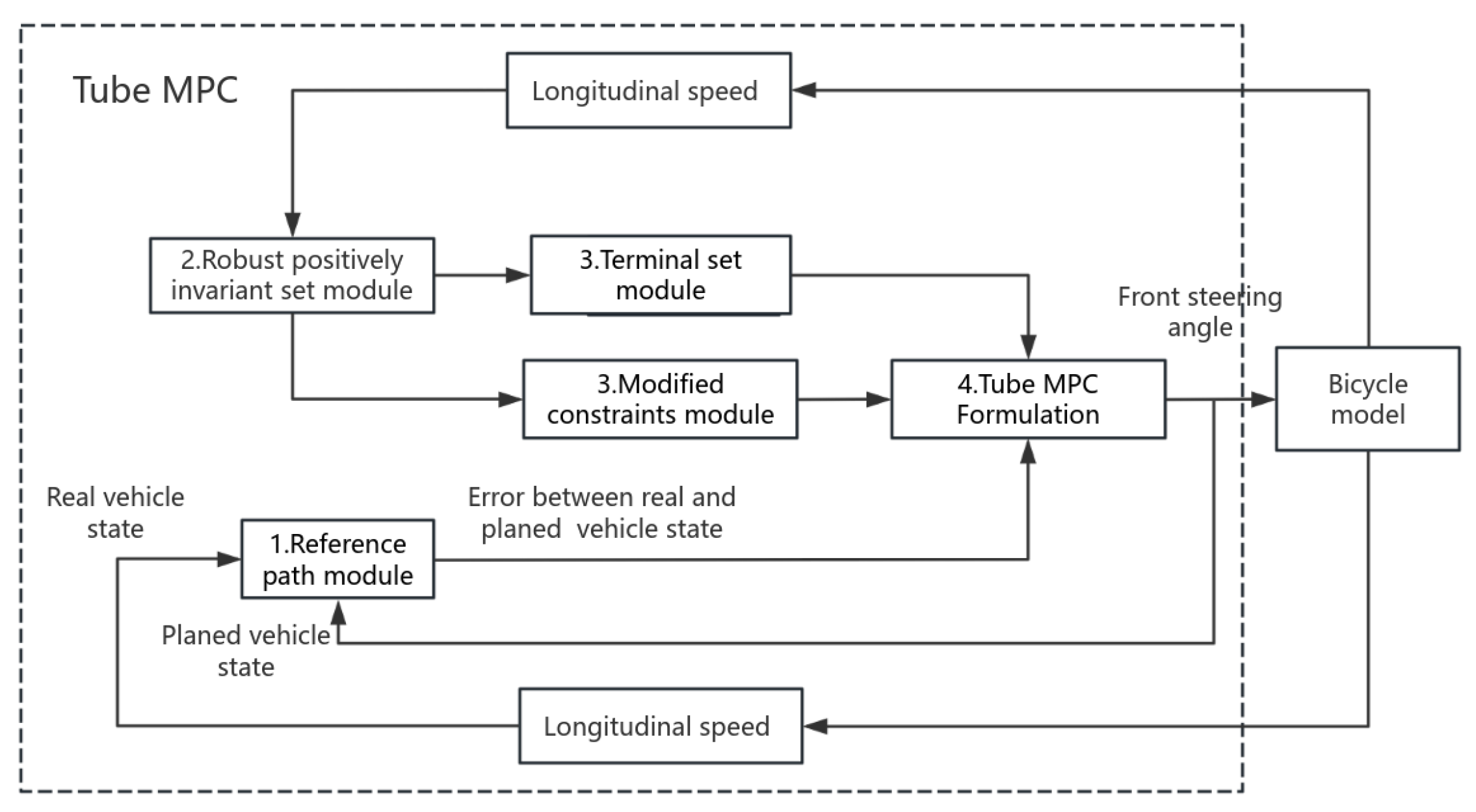
2.1. Control Architecture of Tube MPC

Figure 2 shows the control architecture of tube MPC, which is similar to the control in [30]. Firstly, the reference path module is compared with the real and planned vehicle states, and the errors between them, such as the lateral and yaw error, are then sent to the tube MPC formulation module. Secondly, the robust positively invariant set of the autonomous systems is calculated based on the current longitudinal speed. Then, the terminal sets and constraints are modified based on the robust positively invariant set of the autonomous system, which are treated as the input of the tube MPC formulation module. Finally, the tube MPC formulation module calculates the planned vehicle states and the front steering angle again.

2.2. Set Invariance Theory

In this section, the invariant set theory and robust MPC formulation is introduced for the autonomous system.

In this paper, we assume that $f_a$ expresses the discrete time linear autonomous system.

$${\xi }_{k+1}=f_a\left({\xi }_k,u_k\right)=A{\xi }_k+B{u}_k,$$

(1)

where ${\xi }_k$ and $u_k$ denote the state and the input vectors, respectively. A and B are the control matrix pair, and it is assumed the matrix pair (A,B) will be controllable.

When the autonomous system $f_a$ is perturbed by a bounded additive disturbance, it can be presented as follows:

$$\begin{gathered} {\xi }_{k+1}=f_a\left({\xi }_k,u_k\right)+w_k, \\ {\xi }_k\in \mathrm{\Xi }\subseteq R^n,{\omega }_k\in W\subseteq R^d, \end{gathered}$$

(2)

where $w_k$ is the disturbance vectors, $\mathrm{\Xi }$ and $W$ are the polyhedras that contain the origin.

Definition 1.

(A reachable set with disturbance.) When the autonomous system $f_a$ is perturbed by a bounded, additive disturbance [25], the reachable set of states $S$ is

$$\xi =f_{reach}\left({\xi }_0,u,w\right) \exists {\xi }_0\in S,\exists u\in U,\exists w\in W$$

(3)

where $f_{reach}=f_a\left({\xi }_0,u\right)+w$, and all the states in $S$ are mapped into the reachable set under the map $f_{reach}$ for all inputs $u$ in $U$, as well as the disturbances $w$ in $W$.

Definition 2.

(The robust positively invariant set.) If the set $\epsilon$ meets the requirement detailed below, the set $\epsilon \subseteq \mathrm{\Xi }$ is a robust positively invariant set of states $S$ [25].

$${\xi }_0\in \epsilon \Rightarrow {\xi }_k\in \epsilon ,\forall w_k\in W,\forall k\in N.$$

(4)

Definition 3.

(The maximal robust positively invariant set.) If the set $\epsilon$ is a robust positively invariant set and contains all robust positively invariant sets, the set $\epsilon \subseteq \mathrm{\Xi }$ is the maximal robust invariant set [25].

The Pontryagin difference and Minkowski sum is employed in this paper, and the definition of them can be presented as follows.

The Pontryagin difference of the two polytopes P and Q is expressed in Equation (5):

$$P\mathrm{\theta }Q:=\left\{x\in R^n:x+q\in p,\forall q\in Q\right\}.$$

(5)

The Minkowski sum of the two polytopes P and Q is expressed in Equation (6):

$$P\oplus Q:=\left\{x+q\in R^n:x\in p,q\in Q\right\}.$$

(6)

2.3. Tube MPC Theory

In this section, the framework of the tube MPC for the autonomous system is introduced.

It is assumed that the autonomous system can be expressed as follows:

$$\begin{array}{l}{\xi }_{k+1}=A{\xi }_k+B{u}_k+w_k\\ s.t{\xi }_k\in \mathrm{\Xi }\\ u_k\in U\\ {\omega }_k\in W\end{array}.$$

(7)

The framework of the tube MPC can be divided into two parts. The first part is the nominal system control, which computes the feedforward input of system (7) without disturbance:

$${\overline{\xi }}_{k+i+1}=A{\overline{\xi }}_{k+i}+B{\overline{u}}_{k+i},\forall i=0,1,\cdots ,N-1.$$

(8)

The second part is a state feedback controller that attenuates the state errors between the actual and nominal systems. The state errors between the actual and nominal systems and the feedback input can be presented as follows:

$$e_k={\xi }_k-{\overline{\xi }}_k,$$

(9)

$$\widehat{u}=K{e}_k,$$

(10)

where $K$ is a stabilizing linear feedback gain.

The control input of the tube MPC equals the sum of the feedforward and feedback inputs.

$$u_k={\overline{u}}_k+\widehat{u}={\overline{u}}_k+K{e}_k.$$

(11)

By putting Equations (9) and (11) into System (7), we can express the actual system with $e_k$ as follows:

$$e_{k+1}=A_r{e}_k+w_k=(A+BK)e_k+w_k,$$

(12)

where $A_r=A+BK$, and there exists a gain K that makes it that $A_r$ is a Hurwitz function [27].

If the state ${\xi }_0$ is close to the nominal state ${\overline{\xi }}_0$, Control Law (12) will keep the state within the robust positively invariant set $\epsilon$ for the bounded disturbance w. Section 2.4 includes a proposal for an algorithm regarding the computation of the invariant set.

2.4. Computation of the Approximate Invariant Set

To obtain the input of the autonomous system, the maximal robust positively invariant set should be calculated first. In [26], the authors employed MPT to calculate the robust positively invariant set of the non-linear MPC in the autonomous system. As a series of Minkowski sums need to be calculated when the MPT is employed, the computational burden of the robust positively invariant set is big. To reduce the computational burden, this paper adopted a linear programming (LP) method to solve the approximately robust positively invariant set [31].

Based on Definition 2, a robust positively invariant set can be expressed [31] as follows:

$${\epsilon }_{\infty }={\oplus }_{i=0}^{\infty }{A}_r^{i}W,$$

(13)

where ${\epsilon }_s$ is an $\delta$ approximation of the minimal robust positively invariant set ${\epsilon }_{\infty }$.

$${\epsilon }_s={\oplus }_{i=0}^{s-1}{A}_r^{i}W,$$

(14)

where $s\in N_{+}$, and a scalar is $\alpha \in \left[0,1\right)$. In this paper, s is equal to the predict horizon N − 1.

If $A^{s}W\subseteq \alpha W$ is satisfied, then $\epsilon \left(\alpha ,s\right)={(1-\alpha )}^{-1}{\epsilon }_s$ is convex and ${\epsilon }_{\infty }\subseteq \epsilon \left(\alpha ,s\right)$.

The support function of a set $W\subset R^m$, which is evaluated at $a\in R^m$, is defined as follows [31]:

$$h_W(a)=\underset{w\in W}{\sup }{a}^{T}w.$$

(15)

The scalar can be calculated as

$$\alpha \left(s\right)=\underset{i\in I}{\max }\frac{h_w\left(A^s{f}_{\mathrm{i}}\right)}{g_i}.$$

(16)

The approximation of the robust positively invariant set can be expressed as

$$m\left(s\right)=\underset{j\in N+}{\max }({\displaystyle \sum _{i=0}^{s-1}{h}_w\left({\left(A^i\right)}^T{e}_j\right)},{\displaystyle \sum _{i=0}^{s-1}{h}_w\left(-{\left(A^i\right)}^T{e}_j\right)}).$$

(17)

In general, the computation of the minimal robust positively invariant set by LP can be described with Algorithm 1 [31]:

Algorithm 1. Computation of the minimal robust positively invariant set

1: Input $A,W\mathrm{and}\delta \text{>}0$

2: $s\leftarrow 0$

3: Repeat

4: Compute $\alpha ={\alpha }^0(s)$ with Equation (16)

5: Compute $m(s)$ with Equation (17)

6: $s=s+1$

7: Until $\alpha =\delta /(\delta +m(s))$

8: Compute ${\epsilon }_s$ with Equation (14) and $\epsilon (\alpha ,s)={(1-\alpha )}^{-1}{\epsilon }_s$

3. Vehicle Dynamics Model

In this section, a bicycle vehicle dynamics model is developed and simplified for the control design.

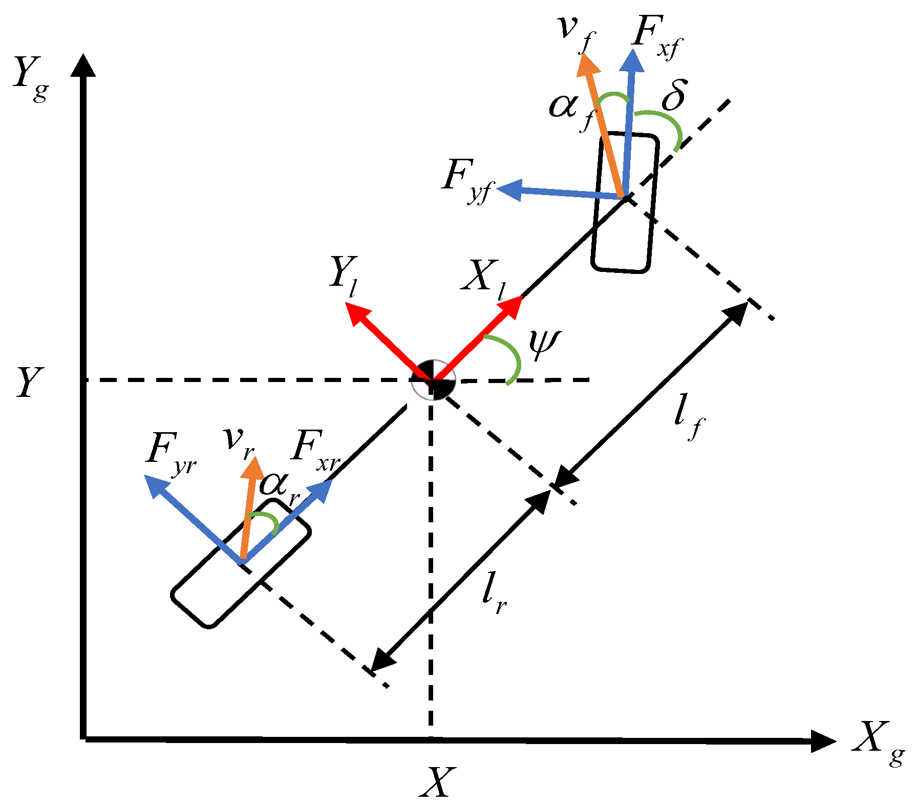
3.1. Lateral Dynamics and Tracking Error Model

As shown in Figure 3, the following set of differential equations were employed to describe the vehicle motion [32]:

$$\ddot{y}=m^{-1}\left(F_{yr}+F_{xf}\sin \delta +F_{yf}\cos \delta \right)-\dot{\psi }\dot{y},$$

(18)

$$\ddot{\psi }=I_z{ }^{-1}\left(l_f{F}_{xf}\sin \delta +l_r{F}_{yf}\cos \delta -l_r{F}_{yr}\right),$$

(19)

where $m$ and $I_z$ are the vehicle mass and inertia moment of vehicle, respectively. $F_{xf}$ and $F_{xr}$ express the force of the front and rear axles along the longitudinal directions, respectively. $F_{yf}$ and $F_{yr}$ represent the force of the front and rear axles along the lateral directions, respectively. $\delta$ expresses the steering angle of the front tire, $\psi$ represents the heading angle, and $\dot{x}$ and $\dot{y}$ represent the velocity of the center mass along the longitudinal $X_l$ and lateral $Y_l$ direction of vehicle coordinate, respectively. $l_f$ and $l_r$ express the longitudinal distance from the center mass to the front and rear axles, respectively.

The state equations of the bicycle model can be described as follows [32]:

$$\dot{x}=A_{k}x+B_k\delta ,$$

(20)

where $x={\left[\dot{y},y,\dot{\psi },\psi \right]}^T$ $B_k={\left[\left(C_{\alpha f}T\right)/m,0,\left(l_f{C}_{\alpha f}T\right)/I_z,0\right]}^T$ $T$ is the sample time.

$$\begin{array}{l}{A}_k=\left[\begin{array}{cccc}-\frac{\left(C_{\alpha f} + C_{\alpha r}\right)T}{m{v}_x}& 0& \frac{\left(l_r{C}_{\alpha r} - l_f{C}_{\alpha f}\right)T}{m{v}_x}& 0\\ 1& 0& 0& 0\\ \frac{\left(l_r{C}_{\alpha r} - l_f{C}_{\alpha f}\right)T}{I_z{v}_x}& 0& \frac{\left(l_r{ }^2{C}_{\alpha r} - l_f{ }^2{C}_{\alpha f}\right)T}{I_z{v}_x}& 0\\ 0& 0& 1& 0\end{array}\right]\\ \end{array}.$$

Equation (20) can be expressed as

$$\dot{x}=f\left(x,\delta \right).$$

(21)

The point on the reference trajectory should satisfy Equation (21) as follows:

$${\dot{x}}_r=f\left(x_r,{\delta }_r\right),$$

(22)

where $x_r={\left[{\dot{y}}_r,y_r,{\dot{\psi }}_r,{\psi }_r\right]}^T$ and ${\delta }_r$ are the reference state and steering angle, respectively.

When one expands Equation (21) at one point of reference trajectory by a Taylor series expansion, then—when only keeping the first-order terms—we can obtain

$$\dot{x}=f\left(x_r,{\delta }_r\right)+\frac{\partial f\left(x,\delta \right)}{x}{|}_{\begin{array}{l}x=x_r\\ \delta ={\delta }_r\end{array}}\left(x-x_r\right)+\frac{\partial f\left(x,\delta \right)}{\delta }{|}_{\begin{array}{l}x=x_r\\ \delta ={\delta }_r\end{array}}\left(\delta -{\delta }_r\right).$$

(23)

When subtracting Equation (22) from Equation (23) and discretizing it with the Forward Euler method, we can obtain

$$\tilde{x}\left(k+1\right)=A_k\tilde{x}\left(k\right)+B_k\tilde{\delta }\left(k\right),$$

(24)

where $\tilde{\delta }=\delta -{\delta }_r$ and

$$\tilde{x}={\left[\left(\dot{y}-{\dot{y}}_r\right),\left(y-y_r\right),\left(\dot{\psi }-{\dot{\psi }}_r\right),\left(\psi -{\psi }_r\right)\right]}^T.$$

(25)

3.2. The Zero Steady-State Model

If the curvature is treated as a disturbance, the model in Equation (24) can be applied to the tube MPC. However, the model in Equation (24) will result in a conservative control. Rajamani et al. [33] developed a method through which to obtain the zero steady-state errors model for Equation (24). The steady state $x_{ss}$ and input ${\delta }_{ss}$ of the model can be calculated as follows:

$$x_{ss}={\left[0,-\frac{l_r}{R}+\frac{l_{r}m{V}^2{ }_x}{2C_r(l_r+l_f)R},0,0\right]}^T,$$

(26)

$${\delta }_{ss}=\frac{L}{R}+K_V\frac{V_{ }{{ }^2}_x}{R},$$

(27)

where $L=l_f+l_r$, $K_V=(l_{r}m/2C_{f}L)-(l_{f}m/2C_{r}L)$, and $R$ is the radius of the reference path. Based on Equations (24), (26), and (27), the zero steady-state model can be obtained [33] as follows:

$$x_{\mathrm{\Delta }}=A{x}_{\mathrm{\Delta }}+B_1{\delta }_{\mathrm{\Delta }},$$

(28)

where $x_{\mathrm{\Delta }}=x-x_{ss}$ and ${\delta }_{\mathrm{\Delta }}=\delta -{\delta }_{ss}$.

4. Collision Avoidance Constraints

The collision avoidance constraints are imposed to ensure the vehicle avoids obstacles and that it does not violate the edges of the road in order to guarantee the safety of the autonomous vehicle.

Road boundary constraint: the road boundary is shrunk to account for the vehicle width, and the vehicle is limited to the shrunk road boundary.

$$R_l\le R_v\le R_u,$$

(29)

where $R_v$ is the center of the vehicle, and $R_l$ and $R_u$ are the lower and upper boundary of the road, respectively.

Obstacle avoiding constraint: this involves the circle obstacles that are in the form ${\left(x-x_o\right)}^2+{\left(y-y_o\right)}^2\le R_o$. The obstacle avoiding constraints can be formulated as

$${\left(x_z-x_o\right)}^2+{\left(y_z-y_o\right)}^2>(R_o+R_1),$$

(30)

where $\left(x_o,y_o\right)$ is the center of obstacles, $\left(x,y\right)$ expresses the point of the obstacle, $R_o$ is the inner radius of obstacles, $x_z$ and $y_z$ express the projection of the invariant set onto the global coordinate system, and $R_1$ is the circumcircle of the vehicle width.

Slip angle constraint: In this paper, it was assumed that the slip angle of the tire is small, and the tire lateral force is approximately a linear function of the slip angle. Therefore, the slip angle of the tire is limited to a certain range.

$$\left|{\alpha }_f\right|\le {\alpha }_{df},$$

(31)

$$\left|{\alpha }_r\right|\le {\alpha }_{dr},$$

(32)

where ${\alpha }_f$ and ${\alpha }_{df}$ are the slip angle and the limited value of the front tires, respectively, and ${\alpha }_r$ and ${\alpha }_{dr}$ express the slip angle and the limited value of the rear tire, respectively.

The above constraints are written in the matrix form as follows:

$$h(\epsilon ,u,w) \le 0,$$

(33)

where $\epsilon$ is the minimal robust positively invariant set, and u and w are the input and the disturbances of autonomous vehicles, respectively.

5. The Tube MPC Optimization Problem

In this section, the disturbances are introduced into the MPC framework to formulate the tube MPC optimization problem. In this paper, it was assumed that the control systems are perturbed by a bounded disturbance $w$.

$$x_{k+1}=A_T{x}_k+B_T{u}_k+w_k.$$

(34)

The tube MPC optimization problem can be described as follows:

$$\begin{array}{l}\underset{u}{\min } f_N={\displaystyle \sum _{k=0}^{N-1}\left(x_k^{T}Q{x}_k^{ }+u_k^{T}R{u}_k\right)}+x_N^{T}P{x}_N^{ }+{\rho }^{T}H\rho \\ s.t x_k\in \overline{x}=x_k\ominus \epsilon k=0,1,\dots ,N-1\\ \mathrm{h}\left(x_k,u_k\right)\le \delta k=0,1,\dots ,N-1\\ u_k\in \overline{u}=u\ominus K\epsilon k=0,1,\dots ,N-1\end{array},$$

(35)

where $\epsilon$ expresses the robust invariant set for the states; $N$ is the predicted horizon; $\rho$ is the slack factor; $\overline{u}$ and $\overline{x}$ express the restricted input constraint and state constraint, respectively; and Q, R, P, and H represent the weights of the appropriate dimension penalizing state tracking error, control action, change rate of control, and violation of the soft constraints, respectively.

The solving process of the tube MPC optimization problem can be described as follows. Firstly, all states are calculated for all inputs and disturbances; specifically, the robust positively invariant set when under additive disturbance conditions is calculated by Algorithm 1. Then, the constraints are tightened to keep the autonomous system meeting the requirement of the constraints when under additive disturbance conditions. In this paper, the tightened constraints are equal to the Pontryagin difference of the original constraints, and the maximal robust positively invariant set is based on Equation (35). Finally, the tightened constraints are introduced into the MPC framework, and the optimal input sequence is computed by solving a tightened constrained optimal control problem at each sampling time. The computed optimal control input sequence and the corresponding predicted vehicle state are stored as the nominal input and state. In the next step, the optimal control problem is solved, starting with new state measurements. From the above description, it can be obtained that the optimization problem’s decision variable is the front tires’ steering input sequence. Though the steering input sequence is the 4 × 1 column vector, it has only one effective dimension.

Note that the proposed linear MPC is based on the simplified linear bicycle model, and it is available when the disturbances make the vehicle go into the linear area. The studies in [30] show that most of the existing disturbances did not make the vehicle go into the non-linear area. Therefore, the proposed linear MPC can adapt to most disturbances. When the simplified linear bicycle model cannot precisely describe the vehicle motion, the proposed linear MPC system is not available. For example, the bicycle model cannot describe the vehicle’s motion on the icy or slippery road precisely. The proposed linear MPC system is not available for the above two conditions.

6. Simulation Results and Discussion

Firstly, a comparison was made between the computation load and characterization of the robust positively invariant set when using the traditional MPT and proposed LP method. Then, the proposed tube MPC system was applied to avoid common disturbance conditions such as state disturbance, uncertain road friction coefficients, and wind disturbance. The performance of the tube MPC system was compared with the traditional MPC system. The vehicle parameters in the simulation are listed in

Table 1. Vehicle parameters.

Mass	1723 kg
Inertia moment	2175 kg/m2
Distance between the front axle and center mass	1.232 m
Distance between the rear axle and center mass	1.468 m
The cornering stiffness of the front tire	66,900 N/Rad
The cornering stiffness of the rear tire	62,700 N/Rad
The initial speed	50 km/h
Friction coefficients $\mu$	0.5
Predictive horizon	20
Control horizon	10
Sample time	0.02 s
State disturbance	$\left|x\right|\le {\left[0.05,0.2,0.005,0.02\right]}^T$
Q	[1, 1; 0, 5]
R	[1]
P	[1, 1; 1, 1]
H	10,000
Limited slip angle of vehicle ${\beta }_d$	${12}^{\circ }$
Limited slip angle of the front and rear tires ${\alpha }_{dr}$	0.25

.

Note that—compared with other controllers such as LQR, fuzzy logic control, and sliding mode control—the traditional MPC has better real-time performance, stability, and robustness [13], and it is widely used in autonomous vehicles. Therefore, this paper compared the proposed tube linear MPC with the traditional MPC instead of with other methods.

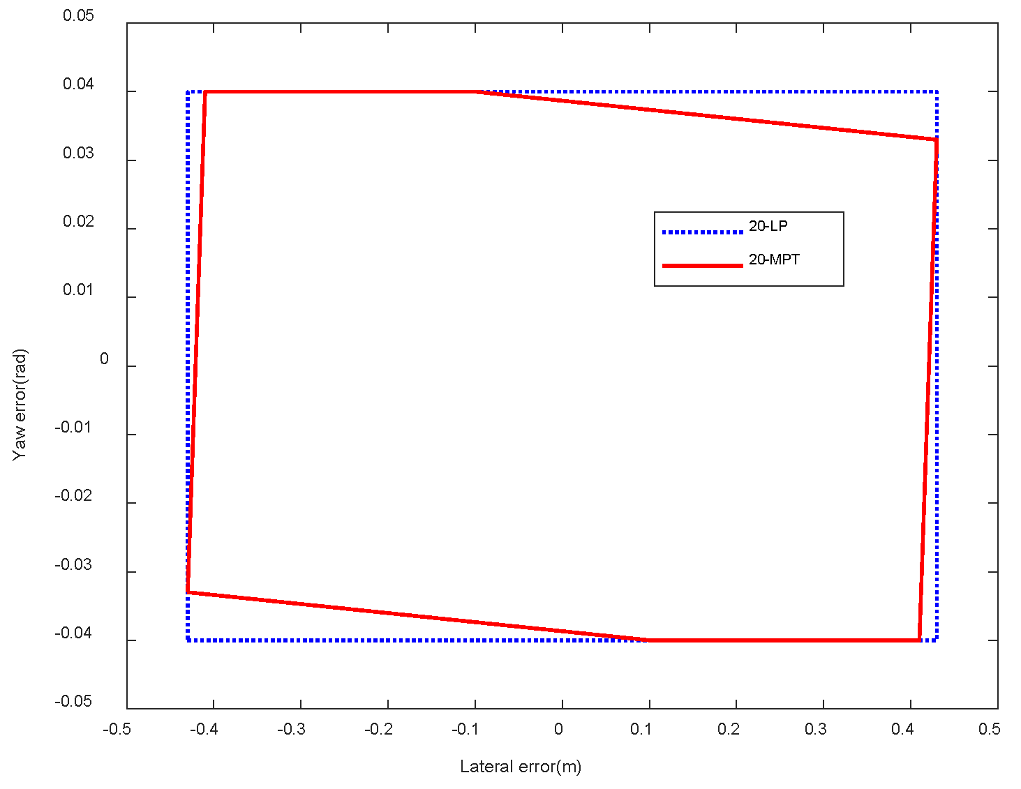
6.1. Comparison of the Robust Invariant Set by the MPT and LP Method

The predicted horizon has a significant effect on the efficiency and accuracy of model predictive control. When the predicted horizon adopts 20 steps, it can trade-off the accuracy and efficiency of the model predictive control well [32]. Therefore, the predicted horizon was set to 20 steps in this paper. Figure 4 shows the 20 steps of the robust invariant sets that were obtained by the LP and MPT methods. In Figure 4, 20-LP and 20-MPT represent the robust invariant sets by the LP and MPT method, respectively. From Figure 4, it can be observed that the robust invariant sets obtained by the LP method is an approximate of that by the MPT method, and the robust invariant sets obtained by the MPT method is a subset of that obtained by the LP method. Based on Definition 3, the robust invariant sets by the LP method is the maximal robust invariant set.

Table 2. Computational burden of the 20-step robust invariant set obtained by the LP and MPT methods.

	LP	MPT
The 20-step robust invariant set	0.03 s	9.6 s

shows the computational burden of the 20 steps of the robust reachable sets by the LP and MPT methods. Evidently, the computational burdens of the 20 steps of the robust reachable set obtained by the LP method were much less than those obtained by the MPT method. In general, the robust invariant sets obtained by the LP method were an approximate of that obtained by the MPT method, and the computational burden of the robust invariant sets obtained by the LP method were much less than those obtained by the MPT. The reason can be explained as follows. According to the algorithm of the minimal robust positively invariant set, Algorithm 1 [31], and parameters in Table 1, the minimal robust positively invariant set was obtained by recursively adding the Minkowski sum 80 times (where the s in (17) is 80). However, it must be noted that 29,030 Minkowski sums were employed in the MPT in [34]. The number of the Minkowski sums obtained by the LP method was much less than that obtained by the MPT method.

The proposed tube linear MPC is appropriate for real-time applications. The reasons for this can be explained as follows: (1) The computing power in engineering contexts is stronger than power of the authors’ laptop. (2) Recently, the MPC has been employed for real-time applications. For example, Hosseinzadeh et al. [35] proposed a robust-to-early termination MPC, and simulations were carried out on a F-16 aircraft to demonstrate the effectiveness of the proposed scheme. Feller et al. [36] presented and analyzed a novel class of stabilizing and numerically efficient model predictive control (MPC) algorithms for discrete-time linear systems, and they demonstrated the effectiveness of the proposed approach. Therefore, it is appropriate for real-time applications.

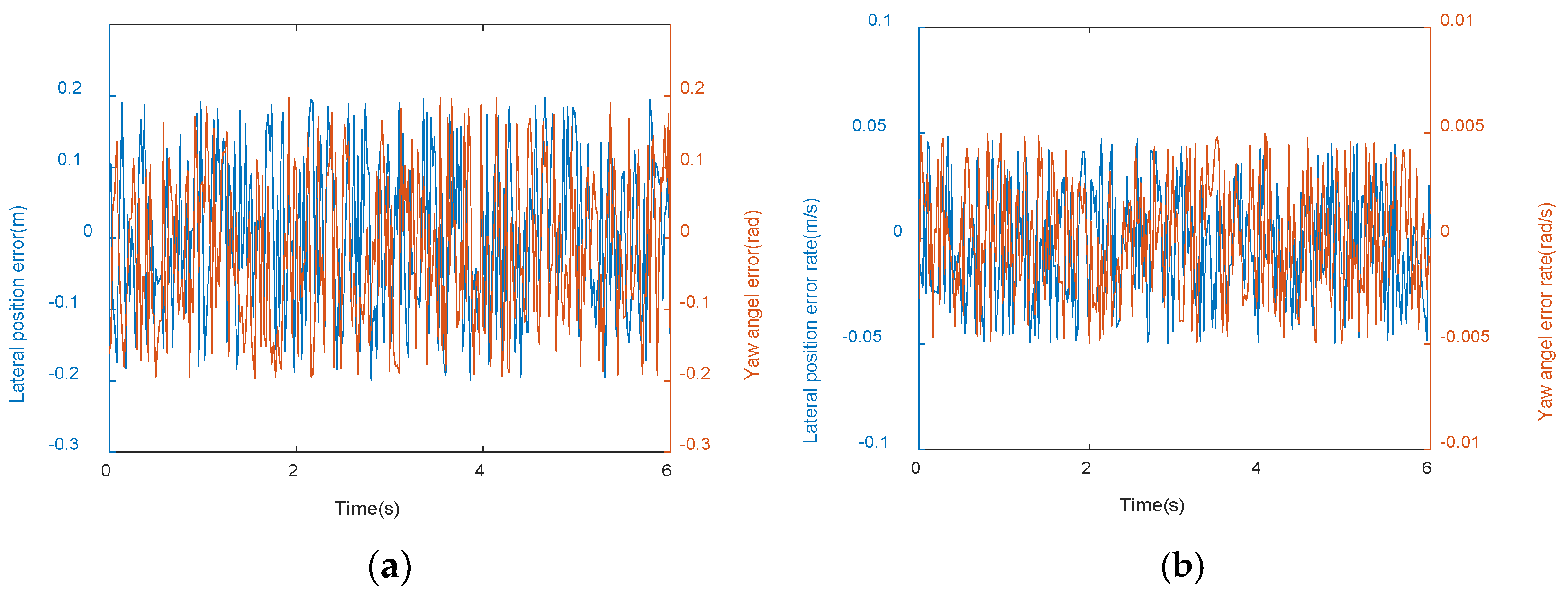
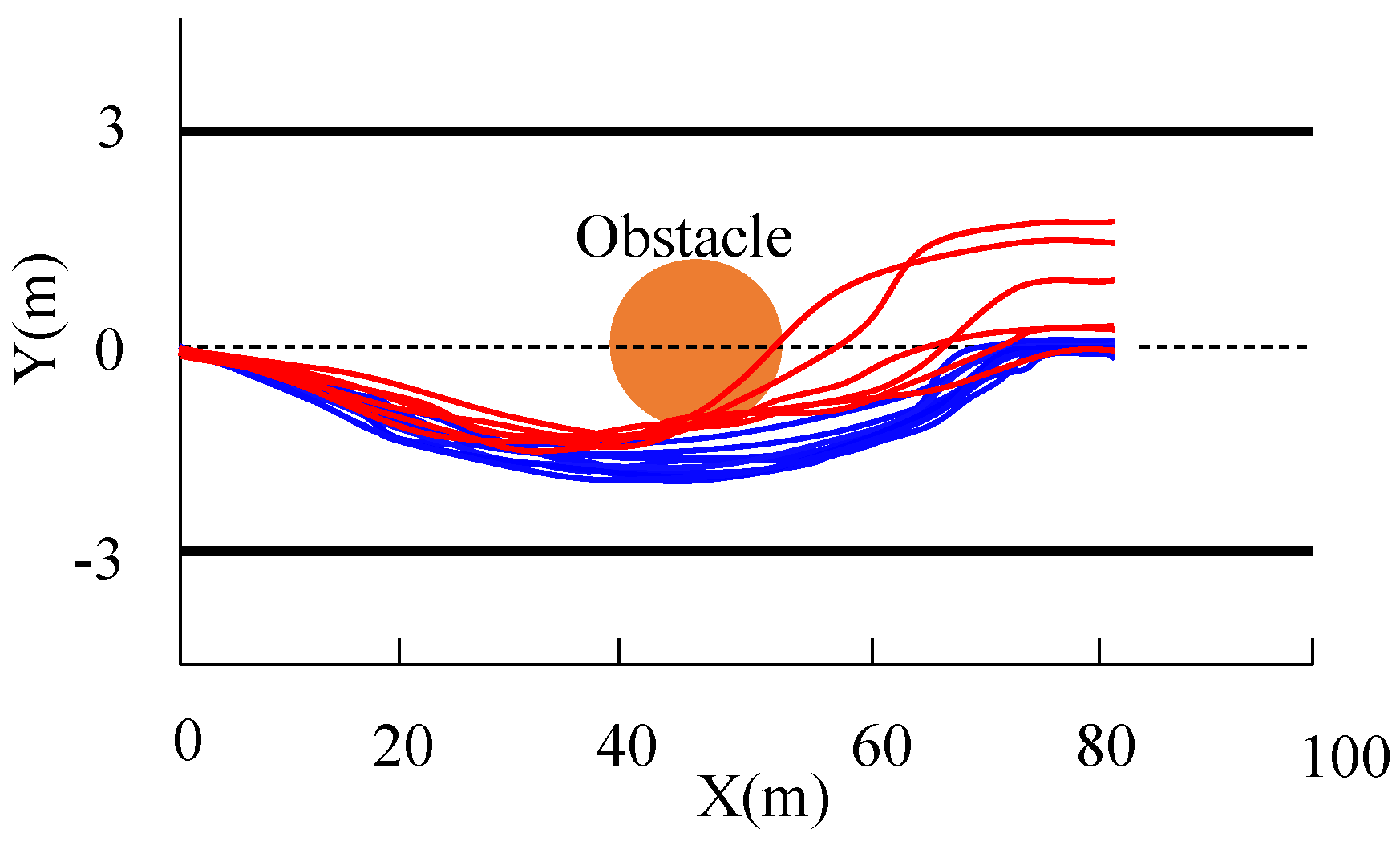
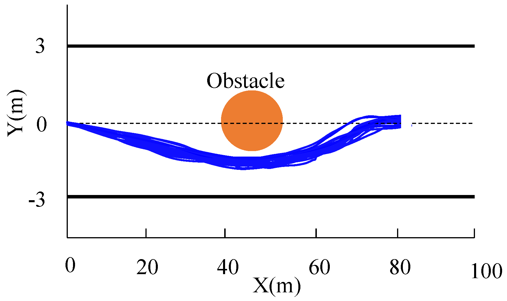
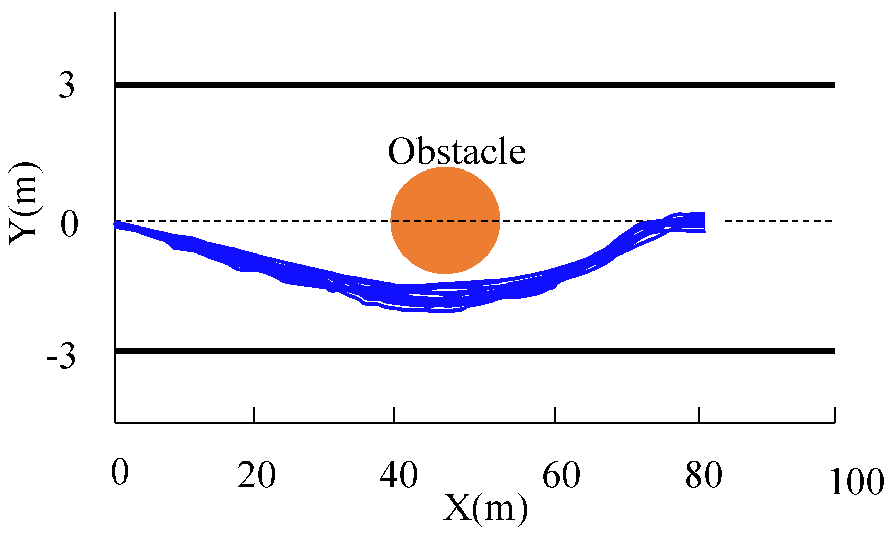
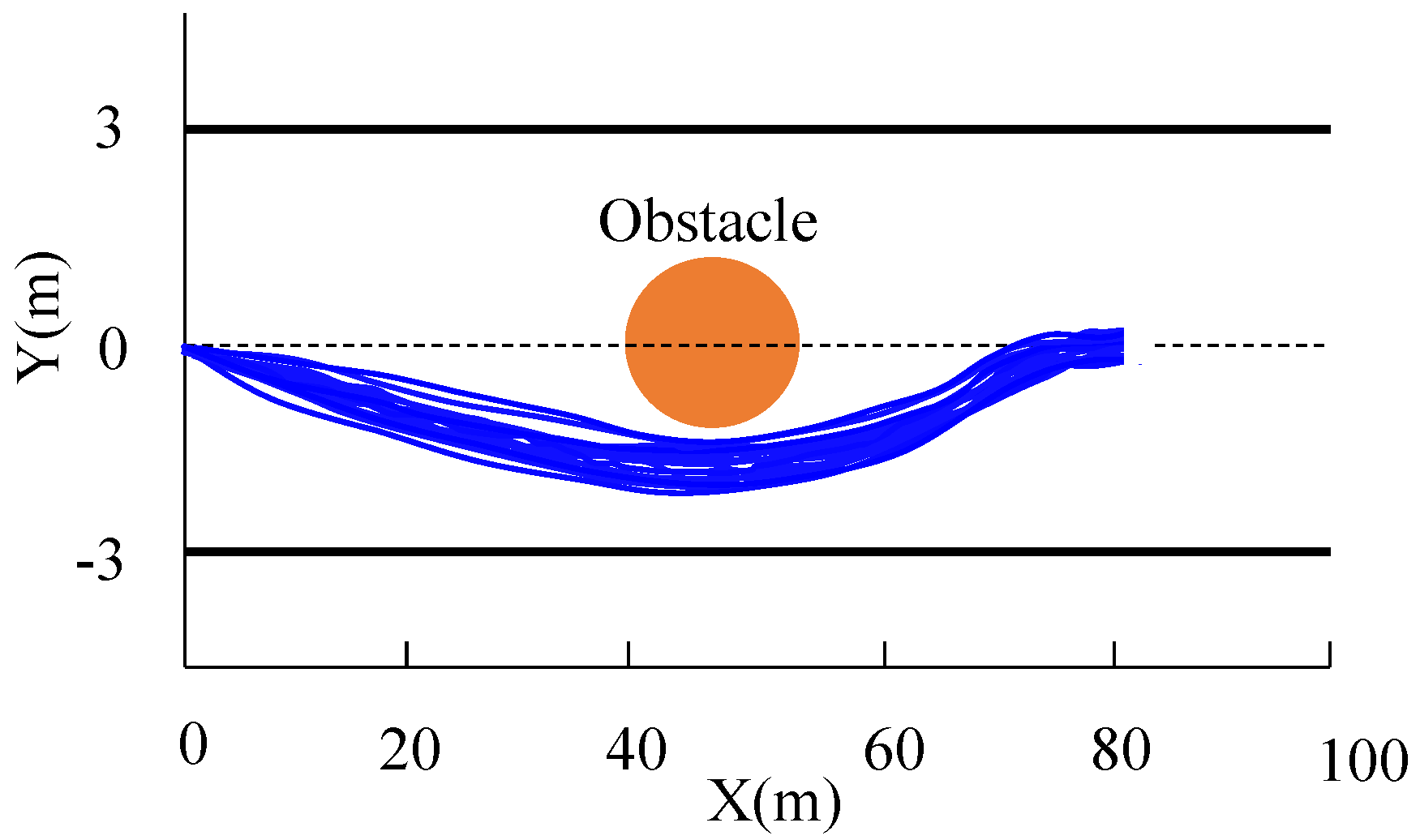
6.2. Performance with State Disturbances

Due to the measurement error and inaccurate vehicle parameters, the actual state may deviate from the nominal state. In other words, the tube MPC system may exhibit state disturbances. In this section, the effectiveness of the tube MPC system when under large state disturbance conditions is demonstrated. In this paper, it was assumed that the random state disturbances had a uniform distribution over the bound [0.05; 0.2; 0.005; 0.02], as shown in Figure 5. In addition, they were added in the simulation model at each sampling time. The results were compared to a traditional MPC without robustness guarantees. A total of 20 trials were run for each controller when subjected to random disturbances. Figure 6 shows the trajectory performances of the traditional MPC when the autonomous vehicle with the traditional MPC avoided one obstacle on the road and returned to the road center. In Figure 6 and Figure 7, the blue and red lines represented the trajectories that successfully avoided the obstacle and failed to avoid the obstacle, respectively.

Table 3. The number of trajectories where the obstacle was avoided successfully when using the proposed and traditional methods.

	Proposed Tube MPC Method	Traditional MPC Method
Number of trajectories	20	14

lists the number of trajectories where the obstacle was avoided successfully when using the proposed tube MPC and traditional MPC methods. The trajectories of the traditional MPC were scattered over a large area, and only 14 trials avoided the obstacle successfully. The tube MPC system was carried out under the same state disturbances and the trajectories performances of the tube MPC method, as shown in Figure 7. Compared with Figure 6 and Figure 7, it can be observed that the range of the trajectories of the tube MPC system was much tighter and that all trajectories successfully avoided the obstacle on the road. The tube MPC system was robust when under state disturbance conditions.

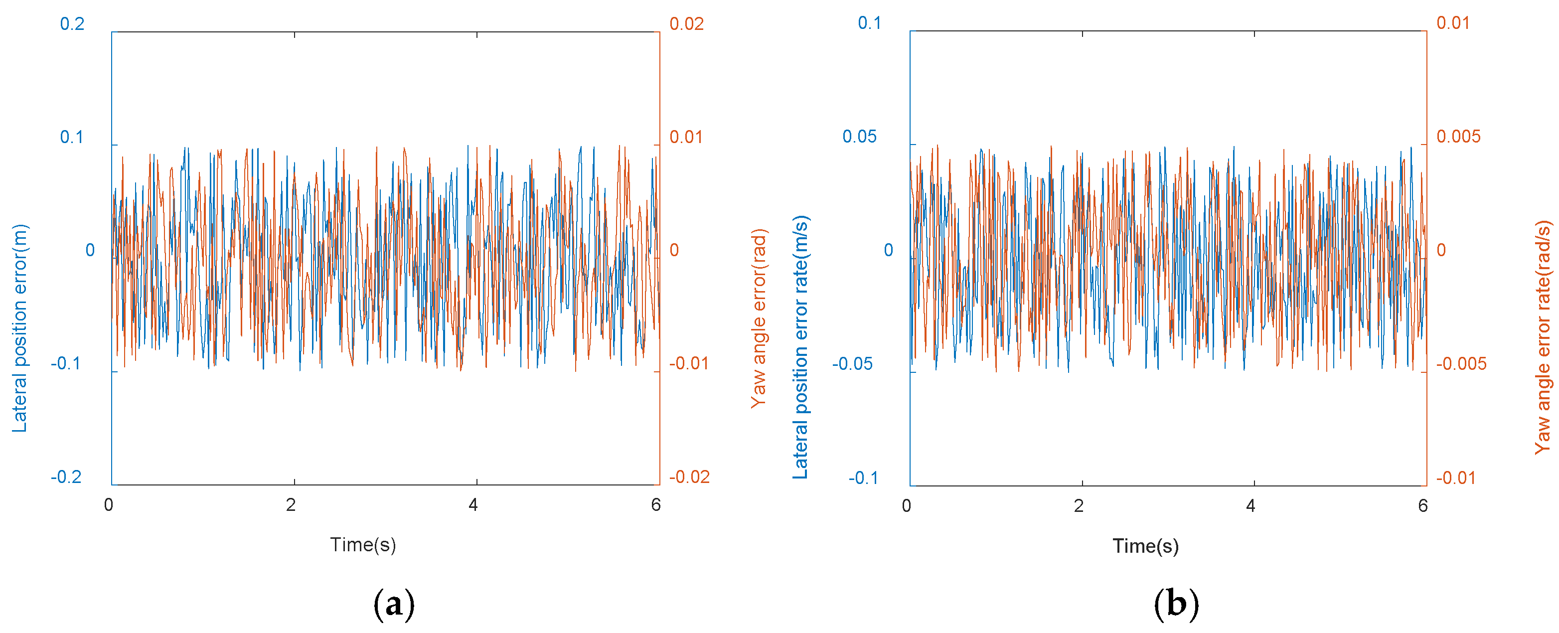
6.3. Performance with Uncertain Tire Road Friction Coefficients

As the surface of the road may contain sand, water, oil pollution, etc., the road friction coefficients may change along the track. In this section, the effectiveness of the tube MPC system under uncertain tire road friction coefficients is demonstrated. The friction coefficient is set to a random value from a uniform distribution over [0.3, 0.7] and by the changes in the simulations. In other words, the nominal friction coefficient is $\overline{\mu }=0.5$ and its bounds are ${\left|\mathrm{\Delta }u\right|}_{\max }=0.2$. The results are compared to a traditional MPC without robustness guarantees. A total of 20 trials were run for each controller with random disturbances. Figure 8 shows the trajectory performances of the traditional MPC under friction coefficient disturbances when the autonomous vehicle avoided one obstacle on the road and returned to the road center. In Figure 8 and Figure 9, the blue and red lines represented the trajectories that successfully avoided the obstacle and failed to avoid the obstacle, respectively.

Table 4. Number of trajectories where the obstacle was avoided successfully when using the proposed and traditional methods.

	Proposed Tube MPC Method	Traditional MPC Method
Number of trajectories	20	16

lists the number of trajectories where the obstacle was avoided successfully when using the proposed tube MPC and traditional MPC methods. The trajectories of the traditional MPC under friction coefficient disturbances were scattered over a large area, and only 16 trials avoided the obstacle effectively. The tube MPC system was carried out under the same friction coefficient disturbance conditions. The trajectory performances of the tube MPC are shown in Figure 9. Compared with Figure 8 and Figure 9, the range of the trajectories of the tube MPC system that were obtained were much tighter, and all of the trajectories successfully avoided the obstacle on the road. The tube MPC system was robust under uncertain tire road friction coefficients.

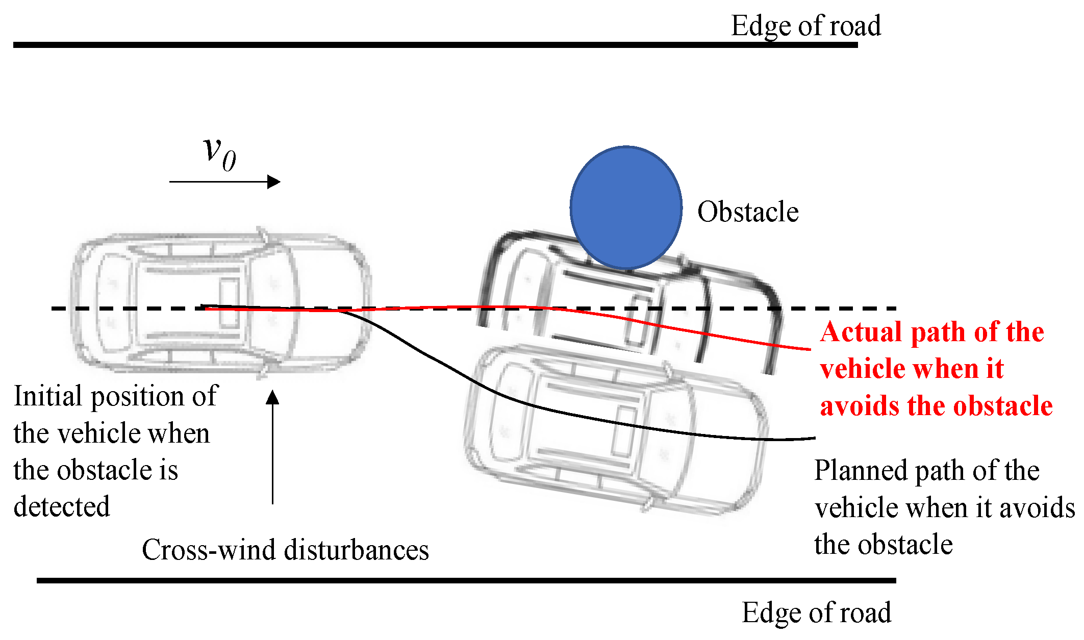
6.4. Performance with Cross-Wind Disturbances

The cross-wind disturbance has an important effect on the tracking performance of autonomous vehicles. The cross-wind disturbance was considered in the tube MPC system, and the effectiveness of the tube MPC system under uncertain cross-wind disturbance is demonstrated. A strong wind disturbance was always present, and this resulted in sharp changes in the direction at the two boundaries. According to ‘the wind speed impact on land and sea’ detailed in the references, the max cross-wind speed reached 19 km/h, which meant that the leaves and smaller twigs were in constant motion. Kvasnica et al. [31] concluded that cross-wind disturbances are a random disturbance and that the state may be perturbed by the bound [0.05; 0.2; 0.005; 0.02] under cross-wind disturbance conditions. In this paper, the state disturbances resulting from the cross-wind were added to the states from the reference path module at each sample time. Figure 10 shows the state disturbance that resulted from the cross-wind disturbance. The results were compared to a traditional MPC without robustness guarantees. A total of 20 trials were run for each controller when subjected to random disturbances. Figure 11 shows the trajectory performances of the traditional MPC under cross-wind disturbances. In Figure 11 and Figure 12, the blue and red lines represented the trajectories that successfully avoided the obstacle and failed to avoid the obstacle, respectively. The trajectories of the traditional MPC were scattered over a large area, and there was a failure in avoiding the obstacle in five of the trials. The tube MPC system was carried out under the same cross-wind disturbances. The trajectory performances of the tube MPC are shown in Figure 12. Compared with Figure 11 and Figure 12, it can be observed that the range of the trajectories of the tube MPC system was much tighter and that all of trajectories successfully avoided the obstacle on the road. The tube MPC system was robust under cross-wind disturbance conditions.

6.5. The Performance with Both Uncertain Wind Disturbance and Friction Coefficients

In this section, both the uncertain wind disturbance and friction coefficients were considered in obstacle avoidance conditions. The effectiveness of the tube MPC system when under both uncertain wind disturbance and friction coefficients is demonstrated. The disturbance range of the cross-wind and friction coefficients were the same as that in Section 6.2 and Section 6.3. The results were compared to a traditional MPC without robustness guarantees. A total of 20 trials were run for each controller with random disturbances. Figure 13 shows the trajectory performances of the traditional MPC. In Figure 13 and Figure 14, the blue and red lines represented the trajectories that successfully avoided the obstacle and failed to avoid the obstacle, respectively. The trajectories of the traditional MPC were scattered over a large area, and there was a failure to avoid the obstacle in eight of the trials. The tube MPC system was carried out under the same cross-wind disturbances. The trajectory performances of the tube MPC are shown in Figure 14. Compared with Figure 13 and Figure 14, it can be observed that the range of the trajectories of the tube MPC system was much tighter and that all of the trajectories successfully avoided the obstacle on the road. The tube MPC system was robust under both uncertain wind disturbance and friction coefficients.

7. Conclusions

This paper proposes a tube linear model predictive controller (MPC) framework for autonomous vehicles in obstacle avoidance conditions. A robust invariant set was calculated with an efficient linear programming (LP) method, and this was used to guarantee that the constraints were satisfied when under common disturbance conditions. The results show that the robust positively invariant sets obtained by the LP method were an approximate of that obtained by the traditional MPT metho. The computational cost of the robust positively invariant sets obtained by the LP method were much less than that obtained by the traditional MPT method. In addition, the traditional MPC and proposed tube MPC framework were employed in obstacle avoidance conditions when subjected to common disturbances. The tracking performances were compared for the traditional MPC and tube linear MPC methods. The results show that the range of the trajectories of the tube MPC system was much tighter and that all the trajectories successfully avoided the obstacle on the road. But the trajectories of the traditional MPC were scattered over a large area and some of the trials failed to avoid the obstacle. The proposed framework can effectively improve the path tracking performance of autonomous vehicles in obstacle avoidance conditions when subjected to common disturbances.

References

1. Li, Z.; Cui, G.; Li, S.; Zhang, N.; Tian, Y.; Shang, X. Lane Keeping Control Based on Model Predictive Control Under Region of Interest Prediction Considering Vehicle Motion States. Int. J. Automot. Technol. 2020, 21, 1001–1011. [Google Scholar] [CrossRef]
2. Liu, Y.; Jiang, J. Optimum path-tracking control for inverse problem of vehicle handling dynamics. J. Mech. Sci. Technol. 2016, 30, 3433–3440. [Google Scholar] [CrossRef]
3. Liu, Z.; Yuan, Q.; Nie, G.; Tian, Y. A Multi-Objective Model Predictive Control for Vehicle Adaptive Cruise Control System Based on a New Safe Distance Model. Int. J. Automot. Technol. 2021, 22, 475–487. [Google Scholar] [CrossRef]
4. Pyun, B.; Seo, M.; Kim, S.; Choi, H. Development of an Autonomous Driving Controller for Articulated Bus Using Model Predictive Control Algorithm with Inner Model. Int. J. Automot. Technol. 2022, 23, 357–366. [Google Scholar] [CrossRef]
5. Yin, J.; Fu, W. Framework of integrating trajectory replanning with tracking for self-driving cars. J. Mech. Sci. Technol. 2021, 35, 5655–5663. [Google Scholar] [CrossRef]
6. Song, Y.; Huh, K. Driving and steering collision avoidance system of autonomous vehicle with model predictive control based on non-convex optimization. Adv. Mech. Eng. 2021, 13, 16878140211027669. [Google Scholar] [CrossRef]
7. Seo, J.H.; Kwon, S.K.; Kim, K.D. A discrete-time linear model predictive control for motion planning of an autonomous vehicle with adaptive cruise control and obstacle overtaking. Adv. Mech. Eng. 2022, 14, 16878132221119899. [Google Scholar] [CrossRef]
8. Calzolari, D.; Schürmann, B.; Althoff, M. Comparison of trajectory tracking controllers for autonomous vehicles. In Proceedings of the 2017 IEEE 20th International Conference on Intelligent Transportation Systems (ITSC), Yokohama, Japan, 16–19 October 2017. [Google Scholar]
9. Cao, J.; Song, C.; Peng, S.; Song, S.; Zhang, X.; Xiao, F. Trajectory tracking control algorithm for autonomous vehicle considering cornering characteristics. IEEE Access 2020, 8, 59470–59484. [Google Scholar] [CrossRef]
10. Qian, Y.; Feng, S.; Hu, W.; Wang, W. Obstacle avoidance planning of autonomous vehicles using deep reinforcement learning. Adv. Mech. Eng. 2022, 14, 16878132221139661. [Google Scholar] [CrossRef]
11. Liu, H.; Yao, Y.; Wang, J.; Qin, Y.; Li, T. A control architecture to coordinate energy management with trajectory tracking control for fuel cell/battery hybrid unmanned aerial vehicles. Int. J. Hydrog. Energy 2022, 47, 15236–15253. [Google Scholar] [CrossRef]
12. He, W.; Tang, X.; Wang, T.; Liu, Z. Trajectory tracking control for a three-dimensional flexible wing. IEEE Trans. Control Syst. Technol. 2022, 30, 2243–2250. [Google Scholar] [CrossRef]
13. Zhai, L.; Wang, C.; Hou, Y.; Liu, C. MPC-based integrated control of trajectory tracking and handling stability for intelligent driving vehicle driven by four hub motor. IEEE Trans. Veh. Technol. 2022, 71, 2668–2680. [Google Scholar] [CrossRef]
14. Rovira-Más, F.; Zhang, Q. Fuzzy logic control of an electrohydraulic valve for auto-steering off-road vehicles. Proc. Inst. Mech. Eng. Part D J. Automob. Eng. 2008, 222, 917–934. [Google Scholar] [CrossRef]
15. Nam, K.; Oh, S.; Fujimoto, H.; Hori, Y. Robust yaw stability control for electric vehicles based on active front steering control through a steer-by-wire system. Int. J. Automot. Technol. 2012, 13, 1169–1186. [Google Scholar] [CrossRef]
16. Guo, J.; Luo, Y.; Li, K. Adaptive coordinated collision avoidance control of autonomous ground vehicles. Proc. Inst. Mech. Eng. Part I J. Syst. Control Eng. 2018, 232, 1120–1133. [Google Scholar] [CrossRef]
17. Norouzi, A.; Kazemi, R.; Azadi, S. Vehicle lateral control in the presence of uncertainty for lane change maneuver using adaptive sliding mode control with fuzzy boundary layer. Proc. Inst. Mech. Eng. Part I J. Syst. Control Eng. 2018, 232, 12–28. [Google Scholar] [CrossRef]
18. Li, S.; Li, Z.; Yu, Z.; Zhang, B.; Zhang, N. Dynamic trajectory planning and tracking for autonomous vehicle with obstacle avoidance based on model predictive control. IEEE Access 2019, 7, 132074–132086. [Google Scholar] [CrossRef]
19. Naus, G.; Van Den Bleek, R.; Ploeg, J.; Scheepers, B.; van de Molengraft, R.; Steinbuch, M. Explicit MPC design and performance evaluation of an ACC Stop-&-Go. In Proceedings of the 2008 American Control Conference, Washington, DC, USA, 11–13 June 2008; IEEE: Piscataway, NJ, USA, 2008; pp. 224–229. [Google Scholar]
20. Sename, O.; Gaspar, P.; Bokor, J. (Eds.) Robust Control and Linear Parameter Varying Approaches: Application to Vehicle Dynamics; Springer: Berlin/Heidelberg, Germany, 2013; Volume 437. [Google Scholar]
21. Tuchner, A.; Haddad, J. Vehicle platoon formation using interpolating control: A laboratory experimental analysis. Transp. Res. Part C Emerg. Technol. 2017, 84, 21–47. [Google Scholar] [CrossRef]
22. Li, S.E.; Jia, Z.; Li, K.; Cheng, B. Fast online computation of a model predictive controller and its application to fuel economy–oriented adaptive cruise control. IEEE Trans. Intell. Transp. Syst. 2014, 16, 1199–1209. [Google Scholar] [CrossRef]
23. Hoffmann, C.; Werner, H. A survey of linear parameter-varying control applications validated by experiments or high-fidelity simulations. IEEE Trans. Control Syst. Technol. 2014, 23, 416–433. [Google Scholar] [CrossRef]
24. Liniger, A.; Zhang, X.; Aeschbach, P.; Georghiou, A.; Lygeros, J. Racing miniature cars: Enhancing performance using stochastic MPC and disturbance feedback. In Proceedings of the 2017 American Control Conference (ACC), Washington, DC, USA, 24–26 May 2017; IEEE: Piscataway, NJ, USA, 2017. [Google Scholar]
25. Mayne, D.Q.; Seron, M.M.; Raković, S.V. Robust model predictive control of constrained linear systems with bounded disturbances. Automatica 2005, 41, 219–224. [Google Scholar] [CrossRef]
26. Gao, Y.; Gray, A.; Tseng, H.E.; Borrelli, F. A tube-based robust nonlinear predictive control approach to semiautonomous ground vehicles. Veh. Syst. Dyn. 2014, 52, 802–823. [Google Scholar] [CrossRef]
27. Seo, J.; Yi, K. Robust Mode Predictive Control for Lane Change of Automated Driving Vehicles; SAE Technical Paper; SAE: Warrendale, PA, USA, 2015. [Google Scholar]
28. Wischnewski, A.; Euler, M.; Gümüs, S.; Lohmann, B. Tube model predictive control for an autonomous race car. Veh. Syst. Dyn. 2022, 60, 3151–3173. [Google Scholar] [CrossRef]
29. Wischnewski, A.; Herrmann, T.; Werner, F.; Lohmann, B. A tube-MPC approach to autonomous multi-vehicle racing on high-speed ovals. IEEE Trans. Intell. Veh. 2022, 8, 368–378. [Google Scholar] [CrossRef]
30. Yu, J.; Guo, X.; Pei, X.; Chen, Z.; Zhou, W.; Zhu, M.; Wu, C. Path tracking control based on tube MPC and time delay motion prediction. Intell. Transp. Syst. 2020, 14, 1–12. [Google Scholar] [CrossRef]
31. Rakovic, S.V.; Kerrigan, E.C.; Kouramas, K.I.; Mayne, D.Q. Invariant approximations of the minimal robust positively invariant set. IEEE Trans. Autom. Control 2005, 50, 406–410. [Google Scholar] [CrossRef]
32. Chen, J.; Tian, G.; Fu, Y. A novel multi-objective tuning strategy for model predictive control in trajectory tracking. J. Mech. Sci. Technol. 2023, 37, 6657–6667. [Google Scholar] [CrossRef]
33. Rajamani, R. Vehicle Dynamics and Control; Springer Science & Business Media: Berlin/Heidelberg, Germany, 2011. [Google Scholar]
34. Kvasnica, M.; Grieder, P.; Baotić, M.; Morari, M. Multi-parametric toolbox (MPT). In Proceedings of the Hybrid Systems: Computation and Control: 7th International Workshop, HSCC 2004, Philadelphia, PA, USA, 25–27 March 2004; Proceedings 7. Springer: Berlin/Heidelberg, Germany, 27 March 2004; pp. 448–462. [Google Scholar]
35. Hosseinzadeh, M.; Sinopoli, B.; Kolmanovsky, I.; Baruah, S. Robust to early termination model predictive control. IEEE Trans. Autom. Control 2023. [Google Scholar] [CrossRef]
36. Feller, C.; Ebenbauer, C. Sparsity-exploiting anytime algorithms for model predictive control: A relaxed barrier approach. IEEE Trans. Control Syst. Technol. 2018, 28, 425–435. [Google Scholar] [CrossRef]
Figure 1. A vehicle colliding with an obstacle due to a cross-wind disturbance.
Applsci 14 02793 g001
Figure 2. Control architecture of tube MPC.
Applsci 14 02793 g002
Figure 3. Schematic of the bicycle model.
Applsci 14 02793 g003
Figure 4. Comparison between the robust invariant set by the LP and MPT methods.
Applsci 14 02793 g004
Figure 5. The state disturbances in the simulation. (a) The lateral position and yaw angle error. (b) The error rate of the lateral position and yaw angle.
Applsci 14 02793 g005
Figure 6. Trajectories of the traditional MPC system when under a random state disturbance.
Applsci 14 02793 g006
Figure 7. Trajectories of the tube MPC system when under a random state disturbance.
Applsci 14 02793 g007
Figure 8. Trajectories of the traditional MPC system under uncertain tire road friction coefficient conditions.
Applsci 14 02793 g008
Figure 9. Trajectories of tube MPC system under uncertain tire road friction coefficient conditions.
Applsci 14 02793 g009
Figure 10. The state disturbances that resulted from the cross-wind disturbance. (a) The lateral position and yaw angle error. (b) The error rate of the lateral position and yaw angle.
Applsci 14 02793 g010
Figure 11. Trajectories of the traditional MPC system when under cross-wind disturbances.
Applsci 14 02793 g011
Figure 12. Trajectories of the tube MPC system when under cross-wind disturbances.
Applsci 14 02793 g012
Figure 13. Trajectories of the traditional MPC system when under both uncertain wind disturbance and friction coefficient conditions.
Applsci 14 02793 g013
Figure 14. Trajectories of the tube MPC system when under both uncertain wind disturbance and friction coefficient conditions.
Applsci 14 02793 g014