Article

Using Transfer Learning and Radial Basis Function Deep Neural Network Feature Extraction to Upgrade Existing Product Fault Detection Systems for Industry 4.0: A Case Study of a Spring Factory

1
Department of Industrial Engineering and Management, National Yunlin University of Science and Technology, Yunlin 640301, Taiwan
2
Department of Computer Science and Engineering, National Chung Hsing University, Taichung 402202, Taiwan
*
Author to whom correspondence should be addressed.
Appl. Sci. 2024, 14(7), 2913; https://doi.org/10.3390/app14072913
Submission received: 29 February 2024 / Revised: 21 March 2024 / Accepted: 24 March 2024 / Published: 29 March 2024

Abstract

:
In the era of Industry 3.0, product fault detection systems became important auxiliary systems for factories. These systems efficiently monitor product quality, and as such, substantial amounts of capital were invested in their development. However, with the arrival of Industry 4.0, high-volume low-mix production modes are gradually being replaced by low-volume high-mix production modes, reducing the applicability of existing systems. The extent of investment has prompted factories to seek upgrades to tailor existing systems to suit new production modes. In this paper, we propose an approach to upgrading based on the concept of transfer learning. The key elements are (1) using a framework with a basic model and an add-on model rather than fine-tuning parameters and (2) designing a radial basis function deep neural network (RBF-DNN) to extract important features to construct the basic and add-on models. The effectiveness of the proposed approach is verified using real-world data from a spring factory.

1. Introduction

In Industry 3.0, automated production became the standard of manufacturing worldwide. Within this model, product fault detection systems are of paramount importance. These systems collect data on machine operations from various sensors and analyze these data to determine whether the manufactured products meet specifications. Thus, product quality can be maintained with minimal human input. Various product fault detection systems exist. For instance, Koscielny et al. [1] and Libal and Hasiewicz [2] performed fault detection in sugar factories using fuzzy neural networks and a binary classification model, respectively. Liu et al. [3] developed a fault detection system for textile products based on the Pearson correlation coefficient and neural networks. Chiu et al. [4] developed a lightweight deep learning model to predict CNC tool wear. More recently, Lee et al. [5] confirmed that if the results of three different convolution kernel-based methods can be ensembled, the fault detection system’s accuracy will be greatly improved. However, in the era of Industry 4.0, cloud and diverse sensor technologies are being introduced to collect production data and implement low-volume high-mix production modes. These changes demand corresponding improvements in existing product fault detection systems.
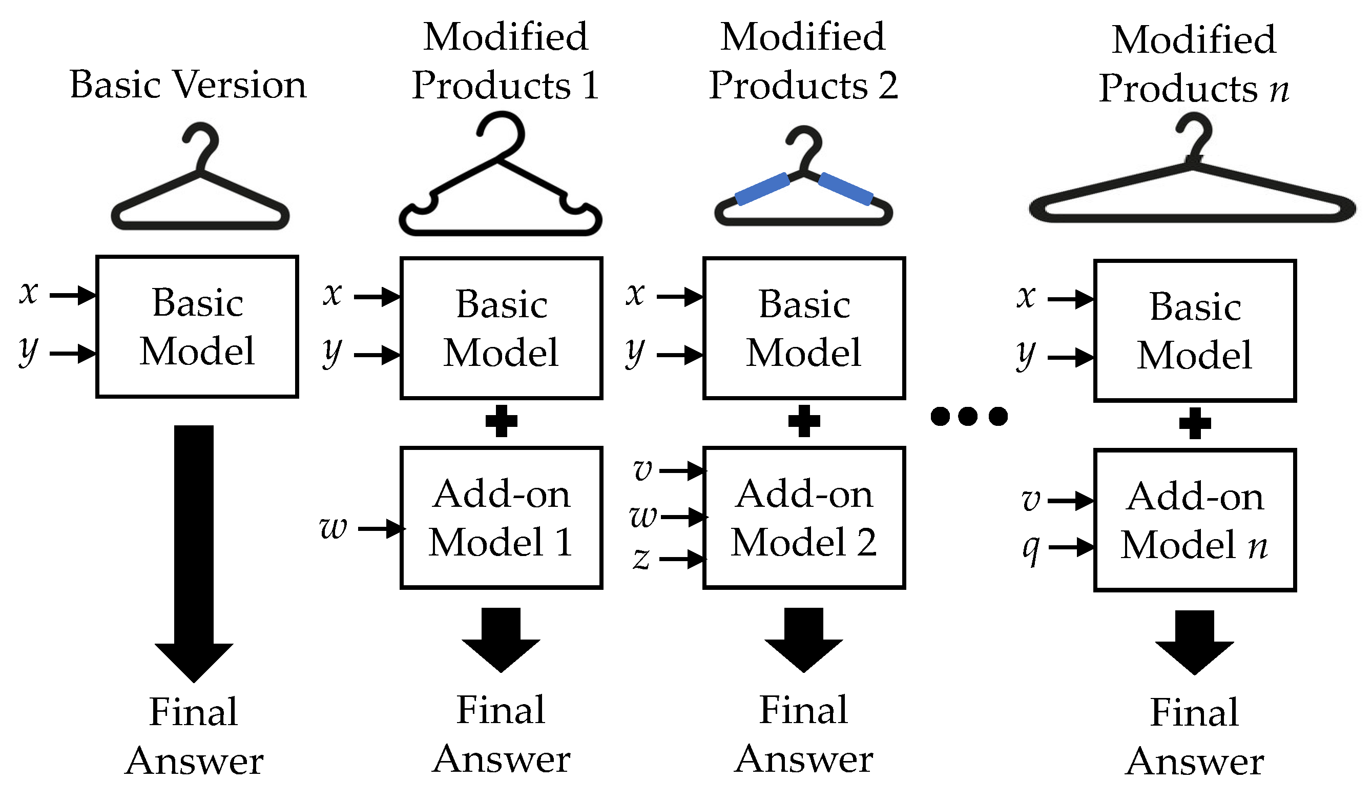
Approaches to upgrading can be roughly divided into four categories. The first category is incorporating cloud and IOT concepts into existing systems [6]. The works in this category are examples of case-by-case design based on the circumstances of the existing system and the environment of the factory. They therefore have little reference value for other factories. The second category of approaches require a rebuilding of product fault detection from scratch. These approaches increase the accuracy of fault detection by incorporating data fusion or hybrid recognition models [7,8,9,10]. The third and fourth categories are tailored to the low-volume, high-mix production modes of Industry 4.0. Specifically, methods in the third category explore means of establishing highly accurate fault detection with little training data. Kuo et al. [11] and Neupane et al. [12] both emphasized the generalizability of this type of approach. However, these methods focus on rebuilding rather than upgrading, which is less cost-effective. The fourth category exploits the high-mix of new production modes, in which similar products of the same basic structure but slightly different details are manufactured in low volumes. For example, consider Figure 1. A clothes-hanger manufacturer will first develop a basic version and then modify it into several different products based on the needs of downstream vendors, such as bottoms of different lengths, notches in the top bars, or non-slip strips on the hanger. This last category of product fault detection depends on transfer learning. A system is first developed for the basic product, and then additional systems for new products are created by fine-tuning the parameters of the existing system. Mazzoleni et al. [13], for instance, investigated the application of fuzzy logic and transfer learning to industrial environments without labeled data, while Raouf et al. [14] considered industrial robots working in different environments.
The application of transfer learning to upgrade existing systems is favored by factories because it requires the least financial and time investments. However, this method still suffers from two major shortcomings. First, the formats of machine operating data may not be the same for similar products, thereby preventing the fine-tuning of existing systems. For example, in Figure 1, the basic version and the two modified products all need only a wire bending machine; however, the third product requires an additional machine to apply the non-slip strip. Thus, the formats for collecting data on the quality of this product differ from those of the other products. Parameter fine-tuning to upgrade the fault detection system is thus not possible. The second shortcoming is associated with how factories manage their fault detection systems. Generally speaking, once a factory establishes a fault detection system, details of the system will be kept in a database for future use. However, if the fault detection system of a basic product is established using deep learning, then the fault detection of the modified product will likely be based on deep learning as well. In the case of production modes with high-mix products, the fault detection database will expand infinitely because it must store many deep learning models with similar structures but slightly different parameters; this will increase the factory’s operating costs. Thus, while the concept of transfer learning for upgrading product fault detection systems hold promise, some issues must still be overcome.
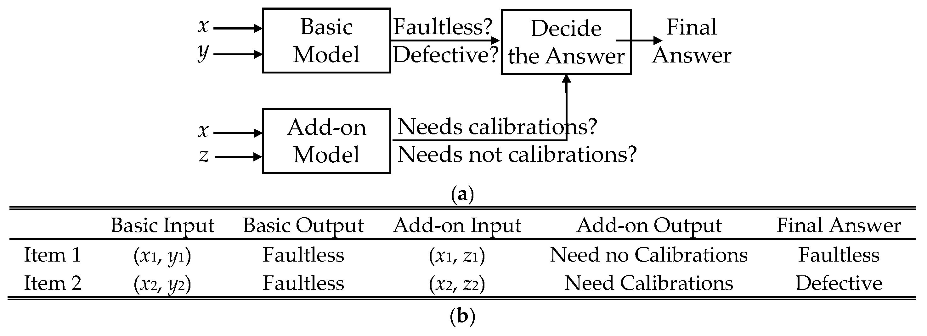
This study proposes two approaches to remedy these issues: (1) While previous methods have realized transfer learning using parameter fine-tuning, we propose creating an add-on model for the basic model. The basic model determines the quality of the basic product, whereas the add-on model assesses the quality of the parts where the new product differs. (2) Existing product fault detection systems use all possible features for modeling; we propose identifying key features that can present product faults before establishing the fault detection model. Figure 2a displays a schematic of the first approach. It does not alter any of the parameters in the basic model but rather corrects the output results of the basic model using the add-on model. In the example shown in Figure 2b, inputting the collected features (x, y) and (x, z) of the first item into the basic model and the add-on model, respectively, produces results in which the item is faultless and the basic model needs no calibrations. We can therefore determine that there is nothing wrong with the product corresponding to the first item. For the second item, inputting the same features into the two models produces results in which the product is faultless and the basic model needs calibrations. We can therefore determine that something is wrong with the product of the second item of data. Furthermore, with the proposed method, the fault detection models of different products can all be extended based on knowledge of the basic model, as shown in Figure 3.
The proposed approaches overcome the shortcomings discussed above as follows. First, input features of the two models can be designed independently; the basic model only needs to consider the features of the basic product, and the add-on model only needs to consider the features that are unique to the modified product. This circumvents the problem of differing data formats. Next, the proposed approach does not adjust the parameters of the basic model but includes an add-on model, so the database will ultimately only contain one basic model and multiple add-on models. This is more efficient than deep learning, as while the basic model must consider a large quantity of information to detect faults in the basic product, the add-on models only consider variations. In other words, the proposed approach effectively reduces the number of model parameters stored in the database. Furthermore, the second approach only uses key features to establish the fault detection model. Existing systems include all features to help clarify the complex associations between machine features and product faults. However, inputting all features into the basic and add-on models not only greatly increases the size of the two models but, more importantly, causes the add-on model to learn information that the basic model already has, which increases training costs unnecessarily.
This paper is the first to explore the inclusion of these approaches to upgrading product fault detection systems. We designed a radial basis function deep neural network (RBF-DNN) and identified key features through training and analysis of the RBF parameters. The proposed RBF-DNN model has a neuron with an RBF as the activation function. RBF has previously been combined with deep learning models to extract key features for modeling for complex time series prediction [4,15]. However, RBF is not limited to time series [16,17]. Thus, the current paper applies this concept to find key input features for product fault detection. We then designed a comprehensive procedure for the creation of add-on models to overcome the insufficiencies of the basic model in detecting faults in new products. Finally, we used production data from a spring factory [11,18] to verify the effectiveness of the proposed approaches.
The remainder of this paper is arranged as follows: Section 2 presents related works, Section 3 introduces the establishment of our framework, Section 4 discusses the results of our experiments, and Section 5 presents our conclusions and future work.

2. Related Works

In this section, we review the existing literature on both machine fault detection systems and product fault detection systems. This is because, in a broad sense, fault detection systems in factory practices generally include those for products and those for the machines, and as the design principles of these two types of algorithms are similar, we introduce them together.
The design methods of fault detection systems can be divided into two categories: statistical analysis methods and data-driven methods. The former compiles the statistics of fluctuations in machine signals and detects faults using these statistics. For instance, Isermanm [19] performed fault detection using standard deviations; they indicated that when the standard deviation does not equal zero, it means that an error has occurred in the product during the production process. Brkovic et al. [20] proposed a fault detection method that compares the residuals of signal amplitudes. Based on principal component analysis, Sarit et al. [21] developed an online fault detection system for industrial fans. Yu et al. [22] combined a corrected reconstruction algorithm with principal component analysis to analyze the sensor data from a nuclear power plant to achieve fault detection. As this methodology was too slow to execute in practice, Yu et al. [23] combined MapReduce with principal component analysis to detect faults in high dimensional data in factories in real time. Xue et al. [24] developed a non-supervisory model aimed at data discrepancies based on k-means and the Apriori algorithm to detect malfunctions in district heating stations. Limaua et al. [25] proposed combining Fourier transform with a sliding window for better resolution in the frequency data. Some researchers have pointed out that the difficulty in implementing this method is setting the size of the window, so Anouar et al. [26] proposed using wavelet analysis to filter data. They filtered and disassembled the data before selecting useful signal features for fault detection. Hartono et al. [27] posited that different types of data have different signal characteristics and important features, so they proposed integrated approaches for feature selection.
Data-driven methods train models individually for product fault detection based on data type. These are currently one of the most popular methods, applied to fields such as electrical systems, industrial processes, and robotics. In earlier research, Wang and Shen et al. [28] proposed applying the Kalman filter for fault detection using the vibration collected from operating machines. However, a number of researchers pointed out that the Kalman filter has two major shortcomings: (1) the standard definitions must be linear, and (2) the fault detection of the model must be fixed. To overcome these issues, Jiang et al. [29] proposed unscented Kalman filter models that can process nonlinear standard definitions to establish their fault detection system. In contrast, Khan et al. [30] added linear regression onto the unscented Kalman filter. With the popularization of artificially intelligent methodology, a growing number of researchers have attempted to increase the complexity of the problems targeted by their approaches. For instance, Nykyri et al. [31] integrated different machine learning methods such as random forest, logistic regression, multilayer perceptron, naive Bayes classification, and linear discrimination to forecast the conditions of a motor in the next ten minutes. Based on fuzzy theory and a hidden Markov model combined with a support vector machine, Mazzoleni et al. [25] developed a system to detect faults in machine health status. Mishra et al. [32] and Nguyen [33], respectively, constructed a neural network and a radial basis function neural network for their target machine signals and then used these models to perform fault detection based on the discrepancies between predicted and actual values. Liu et al. [3] combined Pearson correlation and a neural network to detect faults using the frequencies of sounds made by sewing machines in textile factories. Koscielny et al. [1] employed fuzzy neural networks to perform fault detection based on the temperatures and residue in the evaporation units in a sugar factory. Based on the VGG-16 model, Lilhore et al. [34] proposed a fault detection system that can automatically detect whether a machine is damaged and aid factories in estimating the lifespan of product components. In more recent years, Wen et al. [35] and Chen et al. [36] developed fault detection systems by combining different convolutional neural networks (CNNs) with deep neural networks (DNNs). Hermawan et al. [37] proposed a long short-term memory (LSTM) algorithm based on the lookback principle that, in the event of sensor damage or loss in automated factories, can automatically repair and restore information collected before the damage occurred. Finally, Lee et al. [5] proposed that ensembling different convolution kernel-based methods can greatly improve the accuracy of fault detection.
The above methods verified through experiments that their approach can effectively achieve high-precision single-model fault detection. However, significant shortcomings include the following: (1) Every time the factories work with a different machine (even if it is the same model), they will need to re-collect the machine data and re-establish the model to ensure accuracy. (2) It is costly to collect sufficient data for newly added machines or new error types, making it difficult to train a fault detection model for the target machine. To overcome these shortcomings, the most common approach applies the concept of transfer learning. First, to quickly build models to detect motor faults in different machines of the same type, Kumar and Hati [38] and Skowron [39] used deep learning models and transfer learning. Liu et al. [40] proposed construction chiller defect detection based on transfer learning, claiming that it could be used to establish individual diagnostic models for similar chillers. Chen et al. [41] proposed using TRU fault detection layering technology based on transfer learning to establish models for similar equipment. Li et al. [42] proposed a detection method based on transfer learning and convolutional autoencoders; this was applied to wind turbines. Xu et al. [43] proposed a two-stage digital twin-assisted fault detection method which first predicts the problems that will occur in the machine in a virtual space and builds a detection model for the predicted problems. The model is transferred from the virtual space to the physical space using transfer learning, thereby accelerating the development of fault detection models. To overcome shortages in training data, Cho et al. [44] and Dong et al. [45] developed a fault detection method based on a neural model architecture. Other scholars extended this method. For example, Zhang et al. [46] believed that not all knowledge needs to be transferred, so they proposed transferring only part of the knowledge to the target domain. Chen et al. [41] proposed using the hierarchical structure of convolutional neural networks to perform transfer learning for different fault types. Lee et al. [47] proposed generating adversarial networks to build high-accuracy models in the case of data imbalance. Recently, Wang et al. [48] used the concepts of dual graph neural networks and transfer learning to establish a fault detection model suitable for intelligent manufacturing systems.
Finally, it is worth mentioning that with the rise of the concept of sustainable development, new fault detection systems have been developed based on this concept. For example, Legutko [49] discussed additional factors that should be considered. Patalas-Maliszewska and Łosyk [50] discussed machine maintenance sustainability and developed a corresponding fuzzy neural network model. In addition, considering that most factories already have existing machine fault detection systems, creating new systems is expensive. Therefore, in recent years, most of the efforts in this field have been to extend existing systems to comply with sustainable development. Priority targets such as [51,52,53] all fall into this category of research.

3. Algorithms

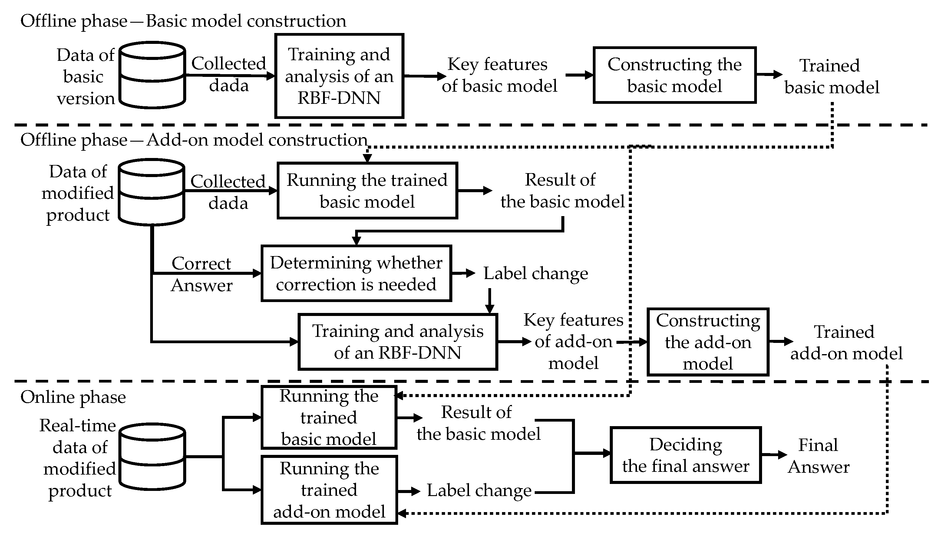
The framework of the product fault detection system developed in this study is shown in Figure 4: it includes two offline phases for the construction of the basic model and the add-on model and an online phase where the basic model and the add-on model operate together. In the beginning of the two offline model construction phases, we employ the radial basis function deep neural network (RBF-DNN) designed in this study and the corresponding parameter analysis methods to identify key features for model construction. This procedure should be applied when the factory has no existing product fault detection system. If they already have their own fault detection system, then the offline phase for basic model construction is ignored and only the second offline phase and the online phase are executed. Below, we introduce the three phases.

3.1. Algorithm for Offline Basic Model Construction

The algorithm designed to construct the basic model in this study comprises two parts: training and analysis of an RBF-DNN to obtain the key features needed to construct the basic model and the means of utilizing these key features to construct the basic model. Note that the content of the first part is more complex, so we further divide our introduction of the first part into three portions: (1) the design concept of the RBF-DNN, (2) the network framework of the RBF-DNN, and (3) the means of analyzing the trained RBF-DNN parameters to obtain the key features.
The RBF-DNN is constructed with a neuron that has an RBF as the activation function added before the DNN. This method has been proven by researchers to be useful in finding the most important input features for modeling. Studies on radial basis function neural networks [16,17] and fuzzy neural networks [54,55], for example, have discussed this issue. For deep learning models, the feasibility of this theory has also been successfully proven on LSTM [15] and RNNs [4]. We therefore extended this concept and added an RBF neuron to an existing model to identify important input features for product fault detection models. We adopted a DNN for our deep learning model rather than the previously discussed LSTM [15] and RNNs [4] because product fault detection models usually process the machine data that they collect from different products separately. In this case, machine data with a sequential format are segmented into independent items of data for processing. LSTM and RNNs, which are dedicated to sequential data, are therefore unsuitable for the target problem. Below, we introduce the proposed RBF-DNN for feature extraction.
The framework of the proposed RBF-DNN is shown in Figure 5, comprising an input layer, an RBF layer, multiple fully connected layers, and an output layer. First, the input layer brings the input features of the model into the neural network. Assuming that the product fault detection system extracts a total of n features from the machine data, expressed as {fb1, fb2, …, fbn}, then the input layer will have n neurons, each responsible for accepting the values of one feature. Next, in the RBF layer, each input layer output will have q neurons responsible for converting it into q probability values. As shown in Figure 6, for example, the RBF centers of three neurons are located at low, middle, and high values. If an input layer value is 0.8, it will be converted into three probabilities, (0, 0.2, 0.7), as shown in Figure 6a. If another input layer value is 0.1, it will be converted into three probabilities, (0.7, 0, 0), as shown in Figure 6b. As for the RBF conversion formula in this paper, we adopted the most common approach, set as
Oij = exp[−(Oinputimij)2/σij2],
where Oij denotes the output of RBF neuron j (jq) of input layer neuron i in the RBF layer; Oinputi represents the output of input layer neuron i; and mij and σij are the mean and standard deviation of this RBF neuron, respectively. After the RBF layer converts the input feature values into probabilities, we next use multiple fully connected layers to establish the nonlinear relationships between these probabilities and the output results. The format of the RBF-DNN output is consistent with that of the product fault detection (i.e., good/bad product or Type 1/Type 2 bad product). For activation of the fully connected layers, considering the fact that these layers explore the nonlinear relationships between the RBF layer outputs and the results, we adopted the tangent sigmoid function below rather than other commonly used functions such as Relu or Leaky Relu:
Oj = tanh(wijIi) + bj,
where Oj represents the output of node j of a layer; tanh(•) denotes the tangent sigmoid function; Ii is the output value of node i of the previous layer; wij is the weight between node i of the previous layer and node j of the current layer; and bj is the bias of node j of the current layer. We let the number of neurons in the output layer equal the number of categories defined by the fault detection system. As this modeling processing is a classification problem, we selected SoftMax as the activation function. Finally, for RBF-DNN training, we chose the classic back-propagation algorithm. As back-propagation is a commonly used algorithm, we do not discuss it in detail here.
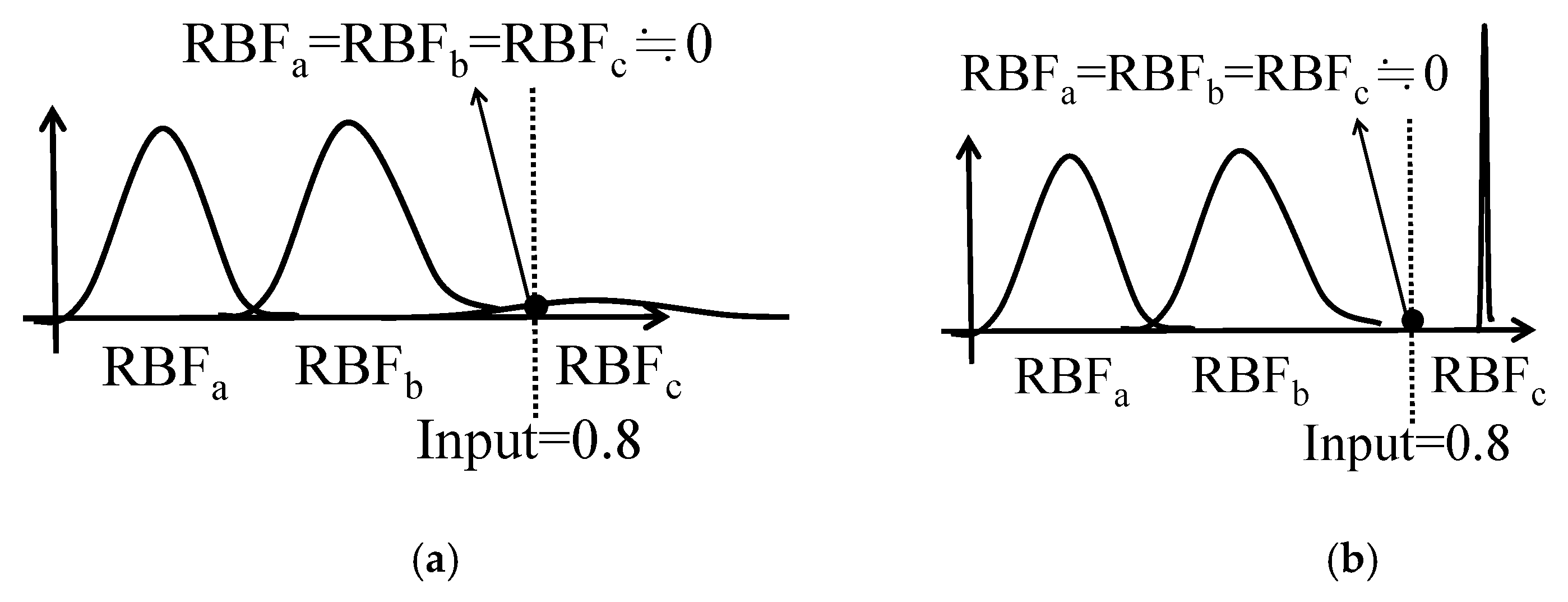
We next discuss how the key input features are obtained using the trained RBF-DNN. Many studies [4,15] have pointed out that when an RBF neuron is placed before a neural network in training, the RBF neuron acts like a switch. For instance, if an input feature uses three RBFs with low, middle, and high centers to perform probability conversions, and it is known that the input feature will have no impact on the output result when it has a higher value, then the highest RBF of the three will adjust its standard deviation to become extremely small or extremely large so that higher values will be converted to zero or fixed probabilities no matter what, as shown in Figure 7. In other words, we need only check whether the RBF neuron output value of each input feature remains at zero or a fixed value to know whether this input feature is useful. If the value of an RBF neuron output fluctuates more widely, this input feature has a greater impact on the output results.
The approach that we designed begins with α RBF-DNNs with different initial weights. Note that multiple RBF-DNNs must be trained because researchers have demonstrated that the important input features that an RBF-DNN selects each time vary with the initial parameters of each network. For this reason, it is necessary to create multiple initial models and then compile the statistics of the results generated by the models before more reasonable results can be produced. After training α RBF-DNNs, we first calculate the standard deviations of the q RBF output values within each RBF-DNN for each input feature. Note that there will be q × α standard deviations for each feature. Then, we calculate the summation of all standard deviations of each feature, rank the values of this summation, and use this to understand the importance ranking of each feature. End users can use this ranked list to select appropriate features based on their needs. For example, suppose that the factory’s computer hardware can only run an AI model with three real-time inputs. In that case, the factory can select the top three from the ranked list to use as key features. On the other hand, if the factory computer has no restrictions, the list is helpful in selecting the features which improve the accuracy of the basic model with the minimum modeling costs.
After using the above method to identify the key features of the basic model, we use these key features to construct the basic model. In selecting the framework of the basic model, the model that each factory uses to perform product fault detection varies. As we cannot test them all, we use the most common artificial neural network to verify the effectiveness of the proposed approach. The inputs of this artificial neural network are the key features that we identified for the basic model, and the output is the fault detection categories defined by the proposed product fault detection system.

3.2. Algorithm for Offline Add-on Model Construction

The algorithm used to construct the add-on model in this study contains a total of three parts: (1) inputting the features of all of the production data obtained from the modified product into the basic model to collect the accuracy rates of the basic model with regard to said data, (2) training and analyzing another RBF-DNN with the production data features of the extended product as the input and the accuracy of the analysis results of the basic model as the output to obtain the key features for add-on model construction, and (3) using the key add-on model features identified in the previous part to construct the add-on model. We next introduce these three parts. Our explanation is aided by the data in Table 1.
In the first part, suppose that the input features of the basic model are {fb1, fb2, …, fbm}, and the features we can obtain from the production data of the modified product are {fe1, fe2, …, fek}; then, we will select the intersection features of the two sets and input them to the basic model for calculation (i.e., the first m columns of Table 1). Note that the production data collected from the modified product may differ from those used in the basic model. There may be more, an equal amount of, or less data. In the first two cases, the features that the basic model needs are all present, so the basic model can operate normally. In the last case, however, the basic model may lack some features. We thus input the value zero for these input features to ensure that the basic model can operate normally, as shown in the second column of Table 1. After the basic model completes its calculations, we obtain the results of the basic model for each item of production data from the modified product, as shown in the “Basic judgment” column of Table 1. We compare this column with the “Real condition” column and define a “Label change” column. As modified products may differ significantly from the basic product, and there is no general solution, we ask factories to define this label change themselves. For instance, if the fault detection results of the basic and modified products in Table 1 are similarly either “good product” or “bad product”, then the label change can be defined as “change” or “do not change”. With the first and second items of data in Table 1, for example, the results of the basic model are the same as those of the modified product, so the label is set as “do not change”. In contrast, with the third and fourth items of data, the results of the basic model are the opposite of those of the modified product, so the label is set as “change”. For a more complex example, suppose that the fault detection results of the basic product are either “good product” or “bad product—too long”, but the factory adds a “bad product—too short” category. In this case, there will be five labels: “do not change”, “good product changed to too long”, “too long changed to good product”, “good product changed to too short”, and “too long changed to too short”. After the label changes for each item of the modified product have been defined, we can proceed to the next step.
The objective of the second part is to train the RBF-DNN again and then analyze this RBF-DNN to obtain the key features needed to construct the add-on model. The RBF-DNN is expected to use k features {fe1, fe2, …, fek} of each item of data in the production data of the modified product as inputs, so the number of input neurons of the RBF-DNN equals k. As for the output layer of the RBF-DNN, the main objective is to output the type of label for each item of data. Thus, the number of neurons in the output layer of this model similarly equals the number of label categories defined by the factory. As the differences between each modified product and the basic product vary, the number of label categories also varies. For this reason, we suggest that users balance the data based on the number of labels before training the RBF-DNN; otherwise, the training results will be poor, and the number of key features obtained from analyzing the model will be inaccurate. The principle, framework, training algorithm, and key feature identification method of this RBF-DNN are all identical to those introduced in the previous section, so we do not discuss them here. Finally, after completing this part of the calculations, we expect to obtain l key features {fadd1, fadd2, …, faddl} needed to construct the add-on model from the RBF-DNN.
The third part of this phase is the construction of the add-on model. To enable the add-on model to smoothly operate with the basic model, we adopted an artificial neural network. The inputs of this network comprise l key features {fadd1, fadd2, …, faddl} identified in the previous part, and the outputs are the label changes defined for each item of data in the first part. Finally, we use back-propagation to complete the training of this add-on model.

3.3. Simultaneous Operation of Basic and Add-On Models Online

In this section, we introduce how the basic and add-on models operate together in the online phase and produce the fault detection results of the current product. Suppose that we obtain k features {fe1, fe2, …, fek} from the production data of the modified product, and the key input features of the basic model and the add-on model are {fs1, fs2, …, fsm} and {fadd1, fadd2, …, faddl}, respectively. We therefore extract the features needed for the basic model and the add-on model from {fe1, fe2, …, fek}. If the features needed by the basic model cannot be found in {fe1, fe2, …, fek}, then we use zero values for the inputs of this dimension. Next, after obtaining the respective outputs of the basic model and the add-on model, we combine the two results and output the fault detection results of the current product. For example, for the case presented in Table 1, the fault detection results of the basic and modified product comprise “good product” and “bad product”, and there are two label changes: “change” and “do not change”. Thus, the first item of data in Table 1 is marked “good product” by the basic model and “do not change” by the add-on model, which means that no product flaws were detected. The outputs of the second, third, and fourth items of data are “good product”, “bad product”, and “good product”.

4. Simulations

In this section, we use a real-world dataset to verify the proposed methodology. The content is divided into four parts: introduction to the dataset and experiment parameters, the performance of basic model construction, the performance of add-on model construction, and the performance of combining the basic model and the add-on model.

4.1. Introduction to Dataset and Experiment Parameters

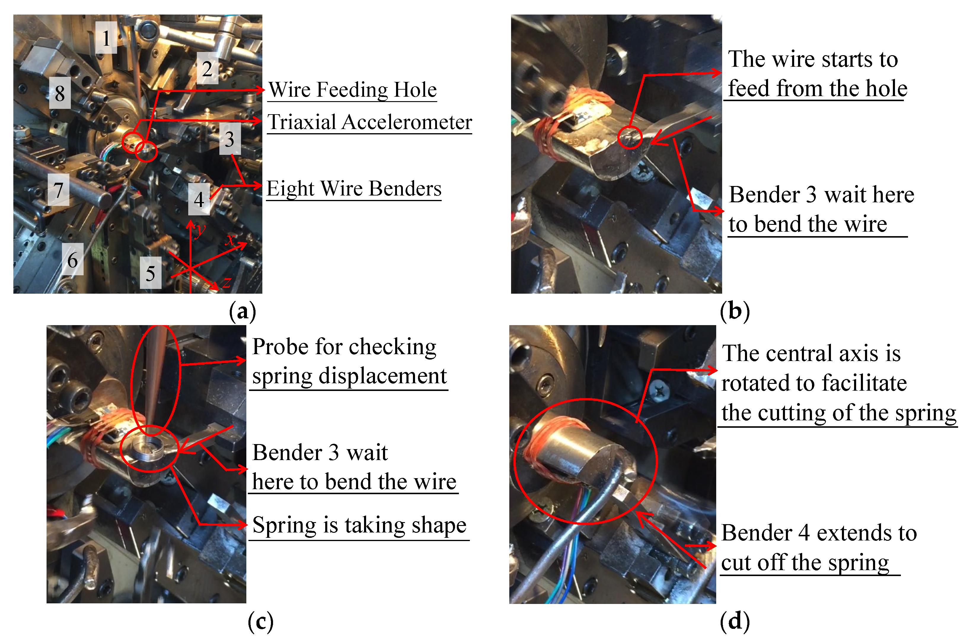
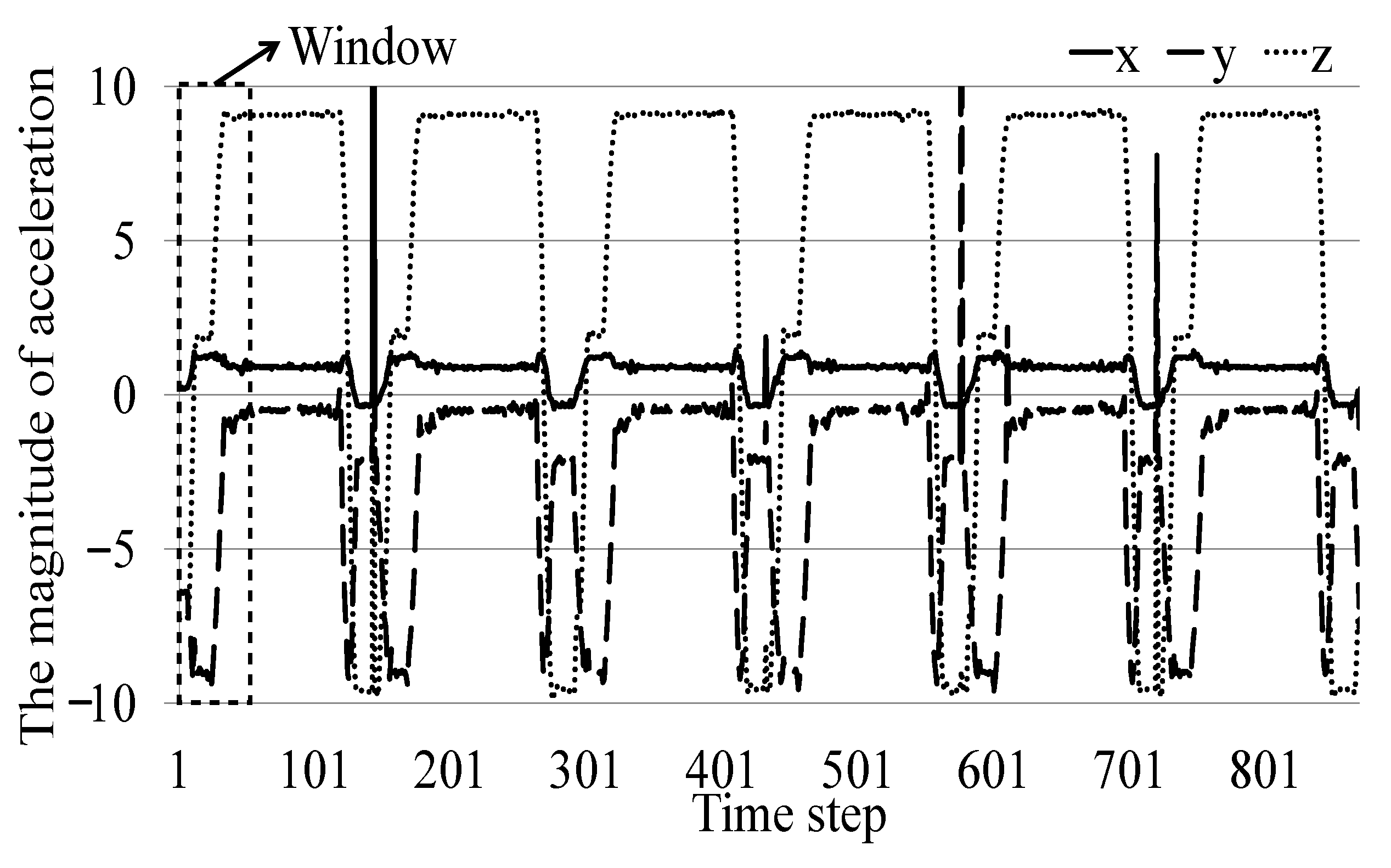
The real-world dataset used in this study was obtained from a spring factory and has been employed by multiple studies in the past [11,18]. Figure 8a shows the architecture of this machine. Figure 8b–d illustrate its operation. It comprises a wire feeding hole in the center column and eight wire benders surrounding it. During operation, a wire is fed from the hole at a fixed speed, and the surrounding wire benders reach out at the right moments to bend the wire and form the spring shape designated by the user. To collect the data, a triaxial accelerometer was installed on the center column, as shown in Figure 8a. This sensor collects acceleration data of the vibrations along the X, Y, and Z axes generated as the wire is fed from the hole and bent by the wire benders. The directions of three axes (X, Y, and Z) are marked on Figure 8a with arrows. The resulting data are displayed in Figure 9: each cycle of variations in acceleration represents the production of one spring. The datasets mentioned in [11,18] include the production data from springs of over a dozen types of lengths. For our research requirement, we only used data from springs that were 171 mm, 181 mm, 188 mm, 189 mm, 190 mm, 210 mm, and 230 mm in length. Those that were 171 mm or 181 mm long were considered to be bad products due to insufficient length; those that were 188 mm, 189 mm, or 190 mm long were considered to be good products; and those that were 210 mm or 230 mm long were considered to be bad products due to excessive length. Based on the characteristics of this dataset, we saw spring length as the difference between the basic product and the modified product and designed two experiments: (1) the basic model only detects good products and bad products that were too long while the add-on model considers three fault categories, and (2) the basic model only detects good products and bad products that were too short while the add-on model considers three fault categories.
The acceleration signal values collected for the spring change periodically (as shown in Figure 9). Therefore, as suggested by previous papers [11,18], we did not use recursive neural networks for modelling, but rather adopted a windowing approach. This method starts by extracting a window for the time series of each acceleration segment and then calculating seven features for each window’s points. The seven features are mean, maximum, energy, root mean square, variance, mean absolute deviation, and standard deviation. As each item of data contains three time series (one for each of the axes, x, y, and z), we ultimately obtained 21 features for each item of data. Based on the needs of our experiment, we set the sizes of the windows and overlaps to be 150 points and 50 points, respectively. Furthermore, as we only considered the length differences between the basic and modified products, we only needed the original accelerator; i.e., there were no issues with increasing or decreasing the features. Thus, in the construction of both the basic model and the add-on model, we considered 21 features.
The four models used in this experiment included (1) the RBF-DNN that determines the key features of the basic model, (2) the basic model itself, (3) the RBF-DNN that determines the key features of the add-on model, and (4) the add-on model itself. We introduce their parameter settings below. First are the two RBF-DNNs in (1) and (3). In the construction phases of the basic and add-on models, 21 features were considered, so the number of input neurons in both RBF-DNNs was 21. Next, regarding the number of neurons in the RBF layer, we referred to the settings of past studies [4,15], in which each input neuron uses three RBF neurons to describe it. Thus, the RBF layer contained a total of 63 neurons. As for the subsequent fully connected layers, we had the number of neurons decrease to a fourth of the former number each time. Thus, the first fully connected layer contained 16 neurons, and the second fully connected layer contained four neurons. Any more fully connected layers would reduce the number to lower than the number of categories considered for product fault detection, so there were no more fully connected layers. The output layer of the RBF-DNN paired with the basic model was expected to have two neurons, whereas that of the RBF-DNN paired with the add-on model was expected to have three neurons. For the training parameters of the two RBF-DNNs, we set 100 epochs, and the learning rate was 0.001. Also, to avoid overfitting, we employed an early stopping procedure in the training process. Finally, we used Adam to avoid local minima. For the training set, we employed the synthesized minority oversampling technique to balance the amounts of data in the different fault detection categories. We selected 70% to serve as the training data and the remaining 30% to serve as the test data. Last of all is the operating environment of these two RBF-DNNs. Both were run in Windows 10, 64-bit, with an AMD Ryzen 9 5900X 12-core processor, 3.7 GHz, and 128 GB of memory. In terms of key feature selection, to verify the high error recognition rate of the proposed method, we assume that the factory does not have any restrictions in terms of hardware and seek features with the highest modeling accuracy and lowest cost. Next are the basic and add-on models themselves in (2) and (4). As we did not want the efficacy of the models themselves to affect our analysis results, we only adopted the simplest method to implement the artificial neural networks of these two models, which was using the NNstart kit provided by Matlab. The default values of the kit were used for all of the parameters of the two artificial neural networks.

4.2. Verification of Basic Model

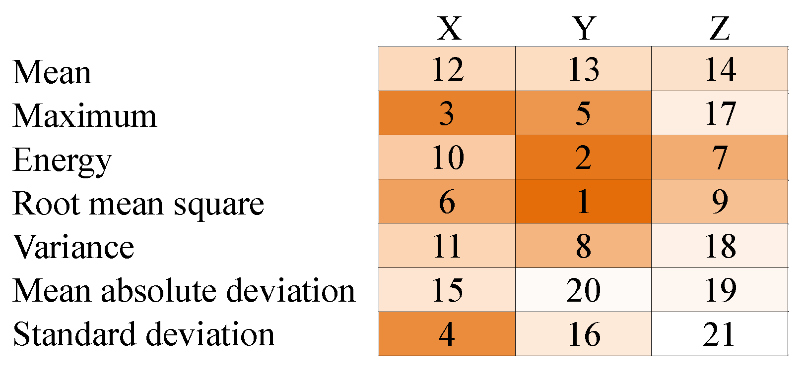
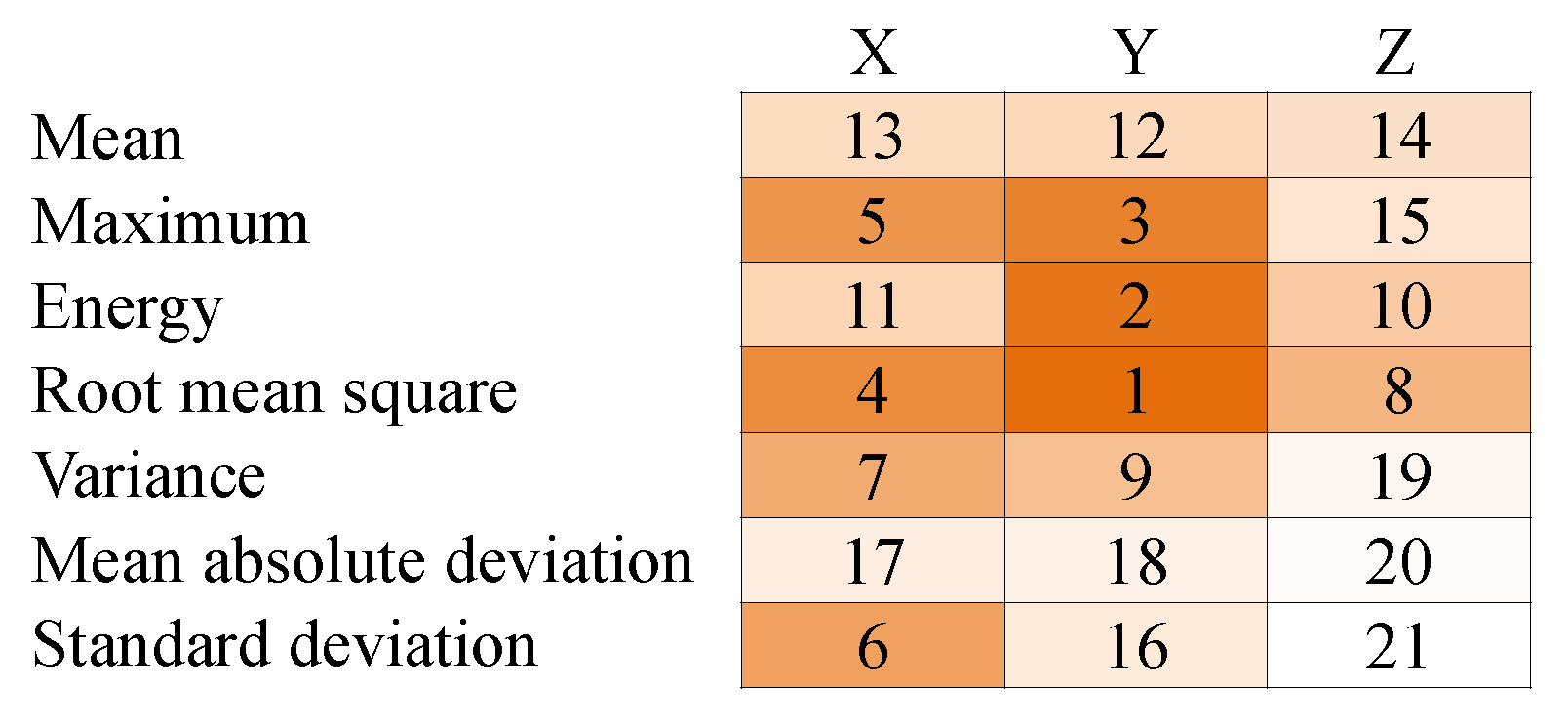
In this section, we verify the efficacy of RBF-DNN for the identification of key features for basic model construction. First, Figure 10 and Figure 11 show the importance ranking of the 21 features found by RBF-DNN for the basic model. Specifically, Figure 10 shows the results of constructing the basic model for products that are good and too long, and Figure 11 presents the results of constructing the basic model for products that are good and too short. Higher rankings are indicated by a darker gradient. It can be seen that the importance ranking is generally consistent with better features on the X axis than those on the Y axis, which are better than those on the Z axis. This is not surprising because the machine used in this experiment mainly moves in the direction of the x axis, and then in the direction of the y axis. Thus, the features identified by the RBF-DNN are ranked accordingly. The z axis is only related to the output movement of the wire, and the signal on the accelerometer remains almost unchanged, so the data represented on this axis are unrelated to product damage.
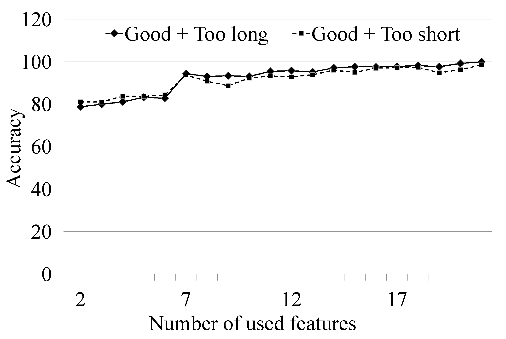
Figure 12 shows the results of experiments on selecting the number of key features. The x axis of these two figures represents the use of the first few features to build the basic model, and the y axis represents the accuracy of the established basic model. This figure shows that x = 7 is the watershed for accuracy changes. Before 7, the accuracy slowly increases, but after 7, it remains stable. Therefore, we select seven modeling features for each of the two sets of experiments.
Table 2 and Table 3 compare the efficacy of the proposed approach (i.e., using the top seven features identified using the RBF-DNN) with other methods for basic model construction. The latter included using all 21 features, with the 8th to 14th most important features (seven in total) identified using the RBF-DNN, the 15th to 21st most important features identified using the RBF-DNN, the 1st to 7th most important features (seven in total) identified using the random forest, the 8th to 14th most important features (seven in total) identified using the random forest, and the 15th to 21st most important features identified using the random forest for basic model construction. Note that this paper uses random forests as the comparison method because they are the most commonly applied for feature extraction in machine learning. The important feature values are set in units of 7 to allow RBF-DNNs to be compared fairly with random forests. Table 2 shows the results of constructing the basic model for products that are good and too long, and Table 3 presents the results of constructing the basic model for products that are good and too short. It is clear from the two tables that, in most cases, the results of using the features ranked as more important by the RBF-DNN were better than those of using less important features. The accuracy of the model constructed using the last seven features was the poorest. These results demonstrate the effectiveness of the proposed RBF-DNN. Next, using all 21 features to construct the basic model produces better results than using only the top seven features identified using the RBF-DNN. However, the computational costs of using all 21 features for modeling are more than three times as high as those of the proposed approach. As both models offer high accuracy, the additional computational costs of the comparative model seem unnecessary. Finally, comparing the RBF-DNN method with a random forest, we can see that the RBF-DNN method can improve modeling accuracy under only seven features. This further confirms the rationality of using the RBF-DNN in the proposed method.

4.3. Verification of Add-On Model Construction

In this section, we explore the efficacy of the add-on model. Note that when a factory builds and uses an add-on model, it is possible to (1) use the method proposed in this paper to build a basic model and (2) directly use the company’s existing method as a basic model. Thus, we conduct two rounds of experimental simulation.
First, we use the proposed method to build a basic model as well as the add-on model. The accuracy of the basic models are 94.4% and 93.8% for the two experiments, respectively. Figure 13 and Figure 14 present the importance rankings of the 21 features found by the RBF-DNN for the add-on model. Specifically, Figure 13 shows the results of identifying products that are too short as well as good products and products that are too long, while Figure 14 displays the results of identifying products that are too long as well as good products and products that are too short. A darker gradient indicates a higher ranking. First, the figures show that for all experiments, energy and root mean square improve significantly compared with the basic model (i.e., Figure 10 and Figure 11). Since the primary learning goal of the add-on model is identifying the difference between the new category of product errors and the old category, the ranking of the place where the difference between the two is the largest will naturally increase. For the machine in this experiment, the length of the spring is related to the amount of time in which the machine outputs the wire and the time in which the machine allows the wire to form a ring. In addition, the length of the wire output time is related to the energy and root mean square of the Z axis. The amount of time the machine allows the wire to form a ring is related to the energy and root mean square of the Y axis, so the rankings of these four features will naturally increase. Second, the importance ranking of most features on the X axis shows a downward trend compared with the ranking of the basic model. This is because the proposed add-on model can take into account less knowledge than the basic model. Therefore, if the basic model learns the features on the X axis (as shown in Figure 10 and Figure 11), then the importance ranking of these repeated features will naturally reduce. Third, the Z-axis features, other than energy and root mean square, are ranked very low in the add-on and basic models. Whether the RBF-DNN is used for the basic or add-on model, it will not select features that are not helpful for modeling. As shown in Figure 10, Figure 11, Figure 13 and Figure 14, Z-axis features other than energy and root mean square are irrelevant to the spring manufacturing process, so they are always ranked low.
Figure 15 shows the experimental results of selecting the number of key features, where the x axis represents the number of the most important features used for add-on model construction and the y axis indicates the accuracy in the resulting add-on model. It is clear that there are turning points in error at x = 7. We therefore selected x = 7 as the number of features for add-on model construction to strike a balance between prediction accuracy and modelling cost.
Table 4 and Table 5 compare the efficacy of the proposed approach with that of existing methods in add-on model construction. The latter again included all 21 features, with the 8th to 14th most important features (seven in total) identified using the RBF-DNN, the 15th to 21st identified using the RBF-DNN for model construction, and the three sets of experiments with the random forest. Table 4 shows the results of identifying products that are too short in addition to products that are good and too long. Table 5 displays the results of identifying products that are too long in addition to products that are good and too short. It is clear that the accuracy of the model constructed using the seven most important features ranked by the RBF-DNN was better than that of using less important features. Next, using all 21 features to construct the add-on model produced slightly better results than using the seven most important features ranked by the RBF-DNN. However, this approach increases the construction costs of the add-on model substantially. Finally, the RBF-DNN outperforms the random forest. This again confirms the rationality of using the RBF-DNN to select features for modeling.
The second scenario simulated uses an existing basic model and an add-on model constructed using the proposed method. We adopt the most intuitive approach to the basic model and directly input all 21 features into a neural network implemented using the suite provided by Matlab R2022b. That is, in Table 2 and Table 3, all 21 dimensions are used as the control group of model inputs. The accuracy of the basic models was 100% and 98.5% for the two experiments, respectively.
First, Figure 16 and Figure 17 show the importance rankings of the 21 features found by the RBF-DNN for the add-on model in this situation. Figure 16 shows the results of identifying products that are too short in addition to products that are good and too long. Figure 17 displays the results of identifying products that are too long in addition to products that are good and too short. Darker gradients indicate higher rankings. Comparing these figures with Figure 13 and Figure 14, we see that the results are almost the same. This is because the main goal of the add-on model is to learn the difference between the new category of product errors and the old category; thus, it is not concerned with information related to the old category on its own. Thus, as long as the product error categories identified by the basic models are the same, the add-on models will be similar. In other words, this experiment confirms that the proposed add-on model can be successfully built on the existing factory model, enabling the factory to upgrade from Industry 3.0 to Industry 4.0 without building a new model.
The remaining experiments included selecting the number of features (Figure 18) and performance verification (Table 6 and Table 7). However, as these results are similar to those depicted in Figure 15 and Table 4 and Table 5, we do not discuss these further.

4.4. Verification of Transfer Learning for the Combination of Basic and Add-On Models

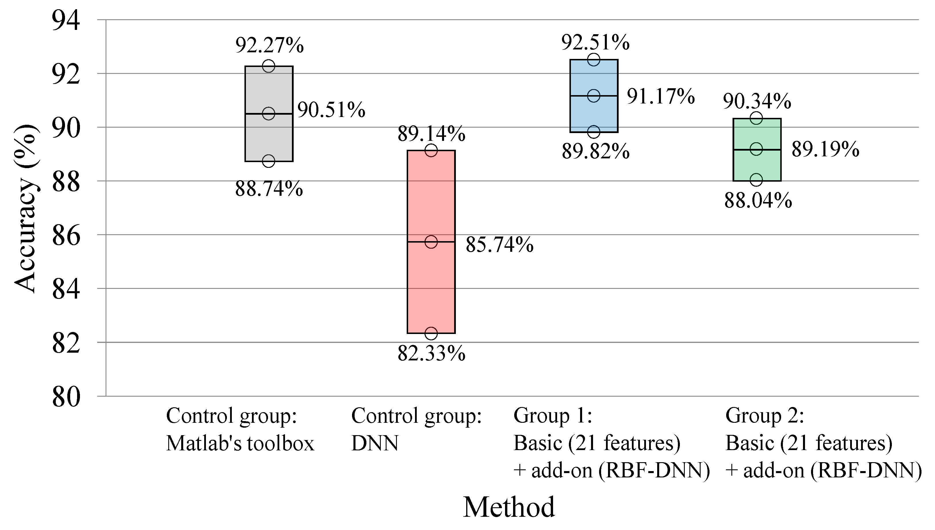
The experimental results shown in Table 8 confirm the effectiveness of transfer learning in the combination of basic and add-on models to upgrade existing fault detection systems. There are three sets of experiments in total, and the values in each set of experiments in the table are the best results of 30 experiments. The first group uses all 21 features to establish three categories of classification models as the control group. These classification models were implemented using Matlab’s NNstart toolbox and the deep neural network kit [56]. The network directly uses the toolbox’s default value. Deep neural networks use six hidden layers and one output layer. Each hidden layer uses the tangent sigmoid function as the activation function, and the last layer uses SoftMax. As for other parameters, we use the Adam accelerator for training and early stops to avoid overfitting. This control group represents the case in which a factory does not use the transfer learning concept and directly uses the old categories with a new error category (which is the most common scenario in practice). The second and third groups are the two sets of experiments we conducted in the above two sections. These two sets of experiments can also be regarded as the results of using basic and add-on models to realize the concept of transfer learning. Note that although the basic model considers different types of errors in these two sets of experiments, they still identify the same three categories of errors with the add-on model. We thus compared these with the control group. The results in Table 8 show the superiority of the experimental results of the control group. This is not surprising, because if all categories of data are given to the model at once, the model will be able to fully consider the differences in the three categories of data when learning and thus obtain the highest recognition accuracy. However, we observe the results of these sets of experiments from the perspective of statistical significance, as shown in Figure 19, where the highest, middle, and lowest values of each set represent the mean + standard deviation, mean, and mean−standard deviation results of 30 experiments. As shown, the numerical ranges between the four groups of experiments overlap, which means that there is no statistically significant difference between them. Therefore, the results of the proposed method are similar to those of the control group, but the proposed model enables factories to upgrade existing models without abandoning the original model or using a low-cost model with fewer features to build an add-on model. This means that the proposed model approach is in line with real-world demands. This conclusion verifies the effectiveness of the transfer learning concept.

4.5. Applicability of Proposed Method in Practice

The approach proposed in this paper can help existing fault detection systems to achieve upgrades through the transfer learning concept without reducing accuracy. This section discusses the applicability of the proposed method in practice from the perspectives of implementation complexity, computational resource requirements, and scalability.
The implementation complexity of the proposed method is described by the algorithm flow chart presented in Figure 4. In the offline stage, the factory only needs to build two models each time to implement the algorithm. In the online stage, the factory only needs to run basic and add-on models once each is finished. This method resembles the actions required by traditional fault detection systems; that is, there is no increase in implementation complexity.
Table 9 presents the computational resource requirements of the target method in the offline and online stages. The average values obtained after conducting the same experiment 30 times are presented. The execution environment is Windows 10, 64-bit, with an AMD Ryzen 9 5900X 12-core processor, 3.7 GHz, and 128 GB of memory. In the offline stage, the execution time of the RBF-DNN is about 30 s, and the Matlab neural kit only takes 5 s to complete. Thus, the computer environment and model running costs are acceptable to most factories. In the online stage, the Matlab neural kit can be completed in about 1 s. This is less than the production time of a single product, so it can be effectively applied for instant fault detection.
As described in Figure 3, the goal of the proposed method is to enable factories to quickly use existing fault detection models to establish extended models. Thus, the approach is inherently scalable, thereby meeting the needs of factories in practice.

5. Conclusions and Future Works

Product fault detection systems are important auxiliary systems for factories and have thus attracted considerable investment. However, as production modes change, many existing systems are becoming invalid. Upgrading existing product fault detection systems will enable factories to move into the era of Industry 4.0 at minimal cost. Existing methods, however, ask factories to completely rebuild their systems. Transfer learning can help factories retain their original systems, but some challenges must still be overcome. This paper proposes two approaches to transfer learning for the upgrading of existing product fault detection systems: (1) using a framework with a basic model and an add-on model and (2) designing an RBF-DNN to extract key features for model construction. We verified the effectiveness of the proposed approach using a real-world dataset. The proposed framework will assist factories in reducing costs associated with upgrading existing product fault detection systems.
The above paragraph summarizes the research motivation and advantages of the proposed framework. However, our approach is subject to certain limitations. Since the framework of this paper is based on the concept of supervised learning, if insufficient error category data are collected by the factory, the framework will not be able to obtain enough training data, leading to system failure. In future work, we plan to include generative AI in this framework to simulate error category data. By using RBF-DNN as a generative AI recognizer, analyzing the critical features captured by this RBF-DNN would also improve the target framework. These additions would likely improve the practical applicability of the proposed framework.

Author Contributions

Conceptualization, C.-H.L. and Y.-C.C.; Data curation, C.-H.L.; Formal analysis, C.-H.L. and Y.-C.C.; Funding acquisition, Y.-C.C. and C.-T.S.; Investigation, C.-H.L. and Y.-C.C.; Methodology, C.-H.L. and Y.-C.C.; Project administration, Y.-C.C. and C.-T.S.; Resources, Y.-C.C. and C.-T.S.; Software, C.-H.L.; Supervision, Y.-C.C. and C.-T.S.; Validation, C.-H.L. and Y.-C.C.; Visualization, C.-H.L. and Y.-C.C.; Writing—original draft, C.-H.L. and Y.-C.C.; Writing—review & editing, C.-H.L. and Y.-C.C. All authors have read and agreed to the published version of the manuscript.

Funding

This research was funded by National Science and Technology Council, grant number 111-2121-M-005-003 and 112-2121-M-005-006.

Institutional Review Board Statement

Not applicable.

Informed Consent Statement

Not applicable.

Data Availability Statement

The datasets presented in this article are not readily available because of a confidentiality agreement signed with Shuai Hao Spring Industrial Co., Ltd. Requests to access the datasets should be directed to the corresponding author.

Conflicts of Interest

The authors declare no conflict of interest.

References

  1. Kościelny, J.M.; Ostasz, A.; Wasiewicz, P. Fault Detection Based on Fuzzy Neural Networks—Application to Sugar Factory Evaporator. IFAC Proc. Vol. 2000, 33, 343–348. [Google Scholar] [CrossRef]
  2. Libal, U.; Hasiewicz, Z. Wavelet based rule for fault detection. IFAC-PapersOnLine 2018, 51, 255–262. [Google Scholar] [CrossRef]
  3. Liu, Z.; Zhou, Z.; Xu, Z.; Tan, D. An adaptive VNCMD and its application for fault diagnosis of industrial sewing machines. Appl. Acoust. 2023, 213, 109500. [Google Scholar] [CrossRef]
  4. Chiu, S.M.; Chen, Y.C.; Kuo, C.J.; Hung, L.C.; Hung, M.H.; Chen, C.C.; Lee, C. Development of Lightweight RBF-DRNN and Automated Framework for CNC Tool-Wear Prediction. IEEE Trans. Instrum. Meas. 2022, 71, 2506711. [Google Scholar] [CrossRef]
  5. Lee, X.Y.; Kumar, A.; Vidyaratne, L.; Rao, A.R.; Farahat, A.; Gupta, C. An ensemble of convolution-based methods for fault detection using vibration signals. In Proceedings of the IEEE International Conference on Prognostics and Health Management (ICPHM), Montreal, QC, Canada, 5–7 June 2023; pp. 172–179. [Google Scholar]
  6. Li, Z.; Wang, Y.; Wang, K.S. Intelligent predictive maintenance for fault diagnosis and prognosis in machine centers: Industry 4.0 scenario. Adv. Manuf. 2017, 5, 377–387. [Google Scholar] [CrossRef]
  7. Mezair, T.; Djenouri, Y.; Belhadi, A.; Srivastava, G.; Lin, J.C. W, A sustainable deep learning framework for fault detection in 6G Industry 4.0 heterogeneous data environments. Comput. Commun. 2022, 187, 164–171. [Google Scholar] [CrossRef]
  8. Vita, F.D.; Bruneo, D.; Das, S.K. On the use of a full stack hardware/software infrastructure for sensor data fusion and fault prediction in industry 4.0. Pattern Recognit. Lett. 2020, 138, 30–37. [Google Scholar] [CrossRef]
  9. Drakaki, M.; Karnavas, Y.L.; Tzionas, P.; Chasiotis, I.D. Recent Developments towards Industry 4.0 Oriented Predictive Maintenance in Induction Motors. Procedia Comput. Sci. 2021, 180, 943–949. [Google Scholar] [CrossRef]
  10. Yan, J.; Meng, Y.; Lu, L.; Li, L. Industrial Big Data in an Industry 4.0 Environment: Challenges, Schemes, and Applications for Predictive Maintenance. IEEE Access 2017, 5, 23484–23491. [Google Scholar] [CrossRef]
  11. Kuo, C.J.; Ting, K.C.; Chen, Y.C.; Yang, D.L.; Chen, H.M. Automatic machine status prediction in the era of Industry 4.0: Case study of machines in a spring factory. J. Syst. Archit. 2017, 81, 44–53. [Google Scholar] [CrossRef]
  12. Neupane, D.; Kim, Y.; Seok, J.; Hong, J. CNN-Based Fault Detection for Smart Manufacturing. Appl. Sci. 2021, 11, 11732. [Google Scholar] [CrossRef]
  13. Mazzoleni, M.; Sarda, K.; Acernese, A.; Russo, L.; Manfredi, L.; Glielmo, L.; Vecchio, C.D. A fuzzy logic-based approach for fault diagnosis and condition monitoring of industry 4.0 manufacturing processes. Eng. Appl. Artif. Intell. 2022, 115, 105317. [Google Scholar] [CrossRef]
  14. Raouf, I.; Kumar, P.; Lee, H.; Kim, H.S. Transfer Learning-Based Intelligent Fault Detection Approach for the Industrial Robotic System. Mathematics 2023, 11, 945. [Google Scholar] [CrossRef]
  15. Chen, Y.C.; Li, D.C. Selection of key features for PM2.5 prediction using a wavelet model and RBF-LSTM. Appl. Intell. 2021, 51, 2534–2555. [Google Scholar] [CrossRef]
  16. Yang, L. Risk Prediction Algorithm of Social Security Fund Operation Based on RBF Neural Network. Int. J. Antennas Propag. 2021, 2021, 6525955. [Google Scholar] [CrossRef]
  17. Zhang, A.; Xie, H.; Cao, Q. The Study of Safety of Ships’ Setting Sail Assessment Based on RBF Neural Network. In Proceedings of the International Conference on Automation, Control and Robotics Engineering, Dalian, China, 19–20 September 2020; pp. 607–611. [Google Scholar]
  18. Chen, Y.-C.; Ting, K.-C.; Chen, Y.-M.; Yang, D.-L.; Chen, H.-M.; Ying, J.J.-C. A Low-Cost Add-On Sensor and Algorithm to Help Small- and Medium-Sized Enterprises Monitor Machinery and Schedule Processes. Appl. Sci. 2019, 9, 1549. [Google Scholar] [CrossRef]
  19. Isermann, R. Fault-Diagnosis Systems-An Introduction from Fault Detection to Fault Tolerance, 1st ed.; Springer: Berlin/Heidelberg, Germany, 2006. [Google Scholar]
  20. Brkovic, A.; Gajic, D.; Gligorijevic, J.; Savic-Gajic, I.; Georgieva, O.; Gennaro, S.D. Early fault detection and diagnosis in bearings for more efficient operation of rotating machinery. Energy 2017, 136, 63–71. [Google Scholar] [CrossRef]
  21. Sarita, K.; Devarapalli, R.; Kumar, S.; Malik, H.; Márquez, F.P.G.; Rai, P.; Malik, H.; Chaudhary, G.; Srivastava, S. Principal component analysis technique for early fault detection. J. Intell. Fuzzy Syst. 2022, 42, 861–872. [Google Scholar] [CrossRef]
  22. Yu, Y.; Peng, M.J.; Wang, H.; Ma, Z.G.; Li, W. Improved PCA model for multiple fault detection, isolation and reconstruction of sensors in nuclear power plant. Ann. Nucl. Energy 2020, 148, 107662. [Google Scholar] [CrossRef]
  23. Yu, W.; Dillon, T.; Mostafa, F.; Rahayu, W.; Liu, Y. A Global Manufacturing Big Data Ecosystem for Fault Detection in Predictive Maintenance. IEEE Trans. Ind. Inform. 2020, 16, 183–192. [Google Scholar] [CrossRef]
  24. Xue, P.; Zhou, Z.; Fang, X.; Chen, X.; Liu, L.; Liu, Y.; Liu, J. Fault detection and operation optimization in district heating substations based on data mining techniques. Appl. Energy 2017, 205, 926–940. [Google Scholar] [CrossRef]
  25. Limaua, F.S.D.; Guedes, L.A.H.; Silva, D.R. Application of Fourier Descriptors and Pearson Correlation for fault detection in Sucker Rod Pumping System. In Proceedings of the IEEE Conference on Emerging Technologies & Factory Automation, Palma de Mallorca, Spain, 22–25 September 2009; pp. 1–4. [Google Scholar]
  26. Anouar, B.A.E.; Elamrani, M.; Elkihel, B.; Delaunois, F. Fault diagnosis of Rotating Machinery using Vibration Measurement: Application of the Wavelet Transform. In Proceedings of the International Conference on Industrial Engineering and Operations Management, Rabat, Morocco, 11–13 April 2017. [Google Scholar]
  27. Hartono, D.; Halim, D.; Widodo, A.; Roberts, G. Bevel Gearbox Fault Diagnosis using Vibration Measurements. In Proceedings of the 2016 International Conference on Frontiers of Sensors Technologies (ICFST 2016), Hong Kong, China, 12–14 March 2016; Volume 59. [Google Scholar]
  28. Wang, Z.; Shen, Y. Kalman Filter-Based Fault Diagnosis. In Model-Based Fault Diagnosis. Studies in Systems, Decision and Control, 1st ed.; Springer: Singapore, 2023; Volume 221, pp. 154–196. [Google Scholar]
  29. Jiang, H.; Liu, G.; Li, J.; Zhang, T.; Wang, C.; Ren, K. Model based fault diagnosis for drillstring washout using iterated unscented Kalman filter. J. Pet. Sci. Eng. 2019, 180, 246–256. [Google Scholar] [CrossRef]
  30. Khan, R.; Khan, S.U.; Khan, S.; Khan, M.U.A. Localization Performance Evaluation of Extended Kalman Filter in Wireless Sensors Network. Procedia Comput. Sci. 2014, 32, 117–124. [Google Scholar] [CrossRef]
  31. Nykyri, M.; Kuisma, M.; Kärkkäinen, T.J.; Junkkari, T.; Kerkelä, K.; Puustinen, J.; Myrberg, J.; Hallikas, J. Predictive Analytics in a Pulp Mill using Factory Automation Data-Hidden Potential. In Proceedings of the IEEE 17th International Conference on Industrial Informatics, Helsinki, Finland, 22–25 July 2019; pp. 1014–1020. [Google Scholar]
  32. Mishra, K.M.; Huhtala, K.J. Fault Detection of Elevator Systems Using Multilayer Perceptron Neural Network. In Proceedings of the IEEE International Conference on Emerging Technologies and Factory Automation, Zaragoza, Spain, 10–13 September 2019; pp. 904–909. [Google Scholar]
  33. Nguyen, N.B. Fault localization on the transmission lines by wavelet technique combined radial basis function neural network. J. Tech. Educ. Sci. 2019, 14, 7–11. [Google Scholar]
  34. Lilhore, U.K.; Simaiya, S.; Sandhu, J.K.; Trivedi, N.K.; Garg, A.; Moudgil, A. Deep Learning-Based Predictive Model for Defect Detection and Classification in Industry 4.0. In Proceedings of the International Conference on Emerging Smart Computing and Informatics, Pune, India, 9–11 March 2022; pp. 1–5. [Google Scholar]
  35. Wen, L.; Li, X.; Gao, L.; Zhang, Y. A New Convolutional Neural Network-Based Data-Driven Fault Diagnosis Method. IEEE Trans. Ind. Electron. 2018, 65, 5990–5998. [Google Scholar] [CrossRef]
  36. Chen, Z.; Deng, S.; Chen, X.; Li, C.; Sanchez, R.V.; Qin, H. Deep neural networks-based rolling bearing fault diagnosis. Microelectron. Reliab. 2017, 75, 327–333. [Google Scholar] [CrossRef]
  37. Hermawan, A.P.; Kim, D.-S.; Lee, J.-M. Sensor Failure Recovery using Multi Look-back LSTM Algorithm in Industrial Internet of Things. In Proceedings of the IEEE International Conference on Emerging Technologies and Factory Automation, Vienna, Austria, 8–11 September 2020; pp. 1363–1366. [Google Scholar]
  38. Kumar, P.; Hati, A.S. Transfer learning-based deep CNN model for multiple faults detection in SCIM. Neural Comput. Appl. 2021, 2021, 15851–15862. [Google Scholar] [CrossRef]
  39. Skowron, M. Analysis of PMSM Short-Circuit Detection Systems Using Transfer Learning of Deep Convolutional Networks. Power Electron. Drives 2024, 9, 21–33. [Google Scholar] [CrossRef]
  40. Liu, J.Y.; Zhang, Q.; Li, X.; Li, G.N.; Liu, Z.M.; Xie, Y.; Li, K.N.; Liu, B. Transfer learning-based strategies for fault diagnosis in building energy systems. Energy Build. 2021, 250, 111256. [Google Scholar] [CrossRef]
  41. Chen, S.W.; Ge, H.J.; Li, H.; Sun, Y.C.; Qian, X.Y. Hierarchical deep convolution neural networks based on transfer learning for transformer rectifier unit fault diagnosis. Measurement 2021, 167, 108257. [Google Scholar] [CrossRef]
  42. Li, Y.T.; Jiang, W.B.; Zhang, G.Y.; Shu, L.J. Wind turbine fault diagnosis based on transfer learning and convolutional autoencoder with small-scale data. Renew. Energy 2021, 171, 103–115. [Google Scholar] [CrossRef]
  43. Xu, Y.; Sun, Y.M.; Liu, X.L.; Zheng, Y.H. A Digital-Twin-Assisted Fault Diagnosis Using Deep Transfer Learning. IEEE Access 2019, 7, 19990–19999. [Google Scholar] [CrossRef]
  44. Cho, S.H.; Kim, S.; Choi, J.-H. Transfer Learning-Based Fault Diagnosis under Data Deficiency. Appl. Sci. 2020, 10, 7768. [Google Scholar] [CrossRef]
  45. Dong, Y.J.; Li, Y.Q.; Zheng, H.L.; Wang, R.X.; Xu, M.Q. A new dynamic model and transfer learning based intelligent fault diagnosis framework for rolling element bearings race faults: Solving the small sample problem. ISA Trans. 2022, 121, 327–348. [Google Scholar] [CrossRef] [PubMed]
  46. Li, X.; Zhang, W.; Ma, H.; Luo, Z.; Li, X. Partial transfer learning in machinery cross-domain fault diagnostics using class-weighted adversarial networks. Neural Netw. 2020, 129, 312–322. [Google Scholar] [CrossRef] [PubMed]
  47. Li, J.; Liu, Y.B.; Li, Q.J. Generative adversarial network and transfer-learning-based fault detection for rotating machinery with imbalanced data condition. Meas. Sci. Technol. 2022, 33, 045103. [Google Scholar] [CrossRef]
  48. Wang, H.; Wang, J.W.; Zhao, Y.; Liu, Q.; Liu, M.; Shen, W.M. Few-Shot Learning for Fault Diagnosis with a Dual Graph Neural Network. IEEE Trans. Ind. Inform. 2023, 19, 1559–1568. [Google Scholar] [CrossRef]
  49. Legutko, S. Industry 4.0 Technologies for the Sustainable Management of Maintenance Resources. In Proceedings of the 2022 International Conference Innovation in Engineering, Minho, Portugal, 28–30 June 2022; pp. 37–48. [Google Scholar]
  50. Patalas-Maliszewska, J.; Łosyk, H. An approach to maintenance sustainability level assessment integrated with Industry 4.0 technologies using Fuzzy-TOPSIS: A real case study. Adv. Prod. Eng. Manag. 2022, 17, 455–468. [Google Scholar] [CrossRef]
  51. Mendes, D.; Gaspar, P.D.; Charrua-Santos, F.; Navas, H. Synergies between Lean and Industry 4.0 for Enhanced Maintenance Management in Sustainable Operations: A Model Proposal. Processes 2023, 11, 2691. [Google Scholar] [CrossRef]
  52. Kaczmarek, M.J.; Gola, A. Maintenance 4.0 Technologies for Sustainable Manufacturing—An Overview. IFAC-PapersOnLine 2019, 52, 91–96. [Google Scholar]
  53. Hadjadji, A.; Sattarpanah Karganroudi, S.; Barka, N.; Echchakoui, S. Advances in Smart Maintenance for Sustainable Manufacturing in Industry 4.0. In Sustainable Manufacturing in Industry 4.0; Springer: Singapore, 2023; pp. 97–123. [Google Scholar]
  54. Wang, Y.; Luo, C. An intelligent quantitative trading system based on intuitionistic-GRU fuzzy neural networks. Appl. Soft Comput. 2021, 108, 107471. [Google Scholar] [CrossRef]
  55. Yao, J.; Lu, B.; Zhang, J. Multi-Step-Ahead Tool State Monitoring Using Clustering Feature-Based Recurrent Fuzzy Neural Networks. IEEE Access 2021, 9, 113443–113453. [Google Scholar] [CrossRef]
  56. Keras 3 API Documentation/Models API/The Sequential Class. Available online: https://keras.io/api/models/sequential/ (accessed on 10 March 2024).
Figure 1. An example of applying the concept of transfer learning to a factory in the Industry 4.0 era.
Applsci 14 02913 g001
Figure 2. Concept of basic and add-on models proposed in this work: (a) schematic, (b) example.
Applsci 14 02913 g002
Figure 3. Concept of extending the basic fault detection models to various modified products.
Applsci 14 02913 g003
Figure 4. The framework of the product fault detection system developed in this study.
Applsci 14 02913 g004
Figure 5. The structure of the proposed RBF-DNN.
Applsci 14 02913 g005
Figure 6. Examples to explain how the RBF layers work. (a) An example for the input layer value is 0.8. (b), An example for the input layer value is 0.1.
Applsci 14 02913 g006
Figure 7. How to use the RBF function to map input values that do not affect the output to 0. (a) Using the RBFc with its standard deviation extremely large. (b) Using the RBFc with its standard deviation extremely small.
Applsci 14 02913 g007
Figure 8. The machine used in this experiment: (a) the structure of the machine, where the numbers 1 to 8 on the picture respectively represent the eight wire benders of the machine (b) the first step in making a spring, (c) the second step in making a spring, and (d) the third step in making a spring.
Applsci 14 02913 g008
Figure 9. An example of using windows to extract features from acceleration signals.
Applsci 14 02913 g009
Figure 10. Importance ranking of 21 features found by RBF-DNN for basic model (good and too long), where darker gradients indicate higher rankings.
Applsci 14 02913 g010
Figure 11. Importance ranking of 21 features found by RBF-DNN for basic model (good and too short), where darker gradients indicate higher rankings.
Applsci 14 02913 g011
Figure 12. Results of selecting the number of key features for the basic model.
Applsci 14 02913 g012
Figure 13. Importance ranking of 21 features found by RBF-DNN for add-on model (good and too long → too short) using proposed method to construct basic model, where darker gradients indicate higher rankings.
Applsci 14 02913 g013
Figure 14. Importance ranking of 21 features found by RBF-DNN for add-on model (good and too short → too long) using proposed method to construct basic model, where darker gradients indicate higher rankings.
Applsci 14 02913 g014
Figure 15. The results of selecting the number of key features for the add-on model in the first situation.
Applsci 14 02913 g015
Figure 16. Importance ranking of 21 features found by RBF-DNN for add-on model (good and too long → too short) for existing basic model, where darker gradients indicate higher rankings.
Applsci 14 02913 g016
Figure 17. Importance ranking of 21 features found by RBF-DNN for add-on model (good and too short → too long) for existing basic model, where darker gradients indicate higher rankings.
Applsci 14 02913 g017
Figure 18. Results of selecting the number of key features for the add-on model in the second situation.
Applsci 14 02913 g018
Figure 19. The results of statistical significance experiments on four main groups.
Applsci 14 02913 g019
Table 1. An example for explaining how add-on models work.
Input Features of
the Basic Model
fb1fb2fb3fbm--Basic
Judgment
Real
Condition
of the Item
Label ChangeAdd on
Judgment
Basic + Add on
Judgment
(Final Judgment)
Features from
Modified Products
fe1-fe2fek-2fek-1fek
Item 1 0.900.41.22.51.3GoodGooddo not changedo not changeGood
Item 2 0.700.61.12.94.1BadBaddo not changechangeGood
Item 3 0.201.30.52.73.5GoodBadchangechangeBad
Item 4 0.101.80.62.62.7BadGoodchangechangeGood
Table 2. Results of constructing basic model for products that are good and too long.
Inputs of the Basic ModelAccuracy
All 21 features100%
1st to 7th most important features identified using the random forest90.2%
8th to 14th most important features identified using the random forest85.3%
15th to 21st most important features identified using the random forest83.7%
1st to 7th most important features identified using RBF-DNN94.4%
8th to 14th most important features identified using RBF-DNN84.1%
15th to 21st most important features identified using RBF-DNN81.1%
Table 3. Results of constructing basic model for products that are good and too short.
Inputs of the Basic ModelAccuracy
All 21 features98.5%
1st to 7th most important features identified using the random forest90.2%
8th to 14th most important features identified using the random forest87.9%
15th to 21st most important features identified using the random forest87.7%
1st to 7th most important features identified using RBF-DNN93.8%
8th to 14th most important features identified using RBF-DNN88.1%
15th to 21st most important features identified using RBF-DNN85.5%
Table 4. Results of constructing add-on model for basic model constructed using proposed method for products that are too short.
Inputs of Basic ModelAccuracy
All 21 features92.3%
1st to 7th most important features identified using the random forest86.3%
8th to 14th most important features identified using the random forest85.1%
15th to 21st most important features identified using the random forest85.9%
1st to 7th most important features identified using RBF-DNN91.7%
8th to 14th most important features identified using RBF-DNN87.3%
15th to 21st most important features identified using RBF-DNN84%
Table 5. Results of constructing add-on model for basic model constructed using proposed method for products that are too long.
Inputs of Basic ModelAccuracy
All 21 features90.1%
1st to 7th most important features identified using the random forest84.7%
8th to 14th most important features identified using the random forest83.9%
15th to 21st most important features identified using the random forest83.5%
1st to 7th most important features identified using RBF-DNN88.7%
8th to 14th most important features identified using RBF-DNN84.3%
15th to 21st most important features identified using RBF-DNN82.7%
Table 6. Results of constructing add-on model for existing basic model for products that are too short.
Inputs of Basic ModelAccuracy
All 21 features93.7%
1st to 7th most important features identified using the random forest91.7%
8th to 14th most important features identified using the random forest89.2%
15th to 21st most important features identified using the random forest88.6%
1st to 7th most important features identified using RBF-DNN92.8%
8th to 14th most important features identified using RBF-DNN90%
15th to 21st most important features identified using RBF-DNN88.3%
Table 7. Results of constructing add-on model for existing model for products that are too long.
Inputs of Basic ModelAccuracy
All 21 features94%
1st to 7th most important features identified using the random forest91.4%
8th to 14th most important features identified using the random forest89.1%
15th to 21st most important features identified using the random forest88.1%
1st to 7th most important features identified using RBF-DNN91.8%
8th to 14th most important features identified using RBF-DNN90.2%
15th to 21st most important features identified using RBF-DNN84.6%
Table 8. Best results of combining basic and add-on models.
Control group: one model (good + too long + too short)
MethodAccuracy
All 21 features + Matlab’s NNstart toolbox94.5%
All 21 features + deep neural network kit93.6%
Group 1: Basic model (good + too long)→add-on model (too short)
MethodAccuracy
Basic (random forest’s 7 features) + add-on (random forest’s 7 features)83.1%
Basic (all 21 features) + add-on (random forest’s 7 features)91.7%
Basic (RBF-DNN’s 7 features) + add-on (RBF-DNN’s 7 features)89%
Basic (all 21 features) + add-on (7 features selected by RBF-DNN)92.8%
Group 2: Basic model (good + too short)→add-on model (too long)
MethodAccuracy
Basic (random forest’s 7 features) + add-on (random forest’s 7 features)83.1%
Basic (all 21 features) + add-on (random forest’s 7 features)89.3%
Basic (RBF-DNN’s 7 features) + add-on (RBF-DNN’s 7 features)88.3%
Basic (all 21 features) + add-on (RBF-DNN’s 7 features)91.9%
Table 9. Computational resource requirements for proposed method.
PhaseOfflineOnline
ActionConstruction of an RBF-DNNConstruction of a neural network using Matlab Running a neural network in Matlab
Time costabout 30 s<5 s<1 s
Disclaimer/Publisher’s Note: The statements, opinions and data contained in all publications are solely those of the individual author(s) and contributor(s) and not of MDPI and/or the editor(s). MDPI and/or the editor(s) disclaim responsibility for any injury to people or property resulting from any ideas, methods, instructions or products referred to in the content.