Article

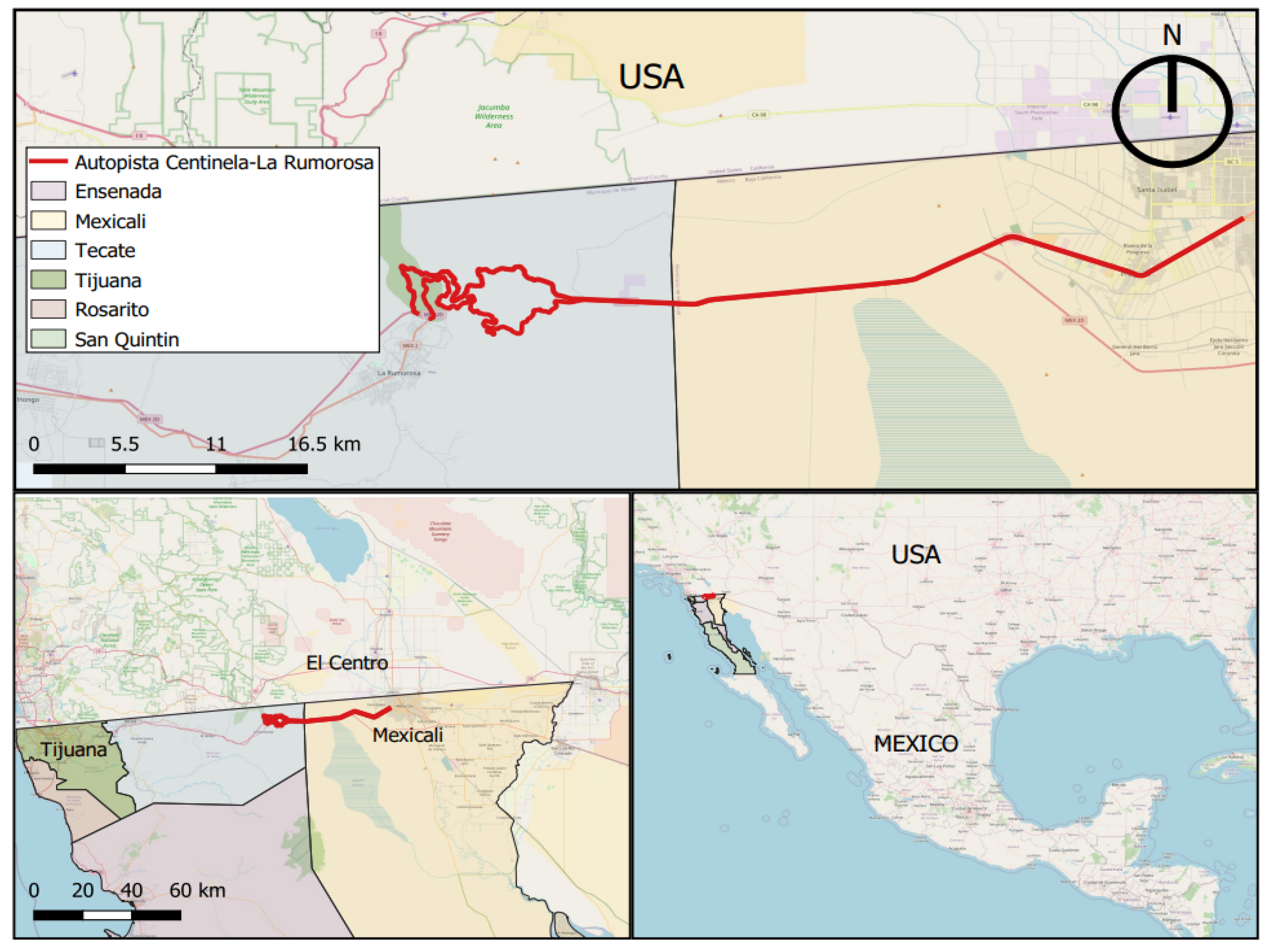
Measurement of Road Transport Emissions, Case Study: Centinela-La Rumorosa Road, Baja California, México

by
Julio Calderón-Ramírez
,
José Manuel Gutiérrez-Moreno
*,
Marco Montoya-Alcaraz
* and
Ángel Casillas
Civil Engineering, Faculty of Engineering, Universidad Autónoma de Baja California (UABC), Mexicali 21100, Mexico
*
Authors to whom correspondence should be addressed.
Appl. Sci. 2024, 14(7), 2921; https://doi.org/10.3390/app14072921
Submission received: 1 March 2024 / Revised: 16 March 2024 / Accepted: 20 March 2024 / Published: 29 March 2024

Abstract

:
Air pollution is a global issue, and the transportation sector is recognized as the third-largest contributor to anthropogenic greenhouse gas emissions. Vehicles emit a range of chemical compounds because of the combustion process. The nature and quantity of these emissions depend on the vehicle’s characteristics, the road, and weather conditions. These emissions require special attention due to the adverse effects contributing to global warming and human health. In this regard, diagnosing and monitoring air quality is crucial for understanding the number of emissions generated by various sources. However, in developing countries, the necessary data for conducting such analyses are not always available. The purpose of this study is to estimate emissions specifically generated from road operations. To achieve this, the HDM-4 calculation tool is utilized to estimate emissions. This tool was applied in Baja California, Mexico, on the Centinela-La Rumorosa highway. The results obtained show that annually, 372.5 tons of pollutant emissions are generated, composed of HC, CO, CO2, NOx, PM, SO2, and PB, covering a mere 128 km of length within a state road network spanning 11,429 km. This highlights the necessity of implementing strategies to reduce the environmental impact generated by vehicular operations on roads in developing countries.

1. Introduction

Since the late 1970s, air pollution has been one of the main topics on global political agendas. Before this period, it was believed that anthropogenic activities were largely responsible for negative environmental changes. However, it was not until then that scientific evidence emerged to support this assertion and the impact it had on a global scale. Nowadays, there is a generally accepted urgency to reduce environmental emissions due to the considerable harm caused by the resulting pollution [1]. This is why environmental pollution, global warming, and the loss of biodiversity are concerns worldwide across different countries. Human activities exacerbate these issues. On the other hand, without raising awareness and taking preventive or mitigating measures, the causes of these problems could lead to irreparable consequences that would affect both our survival and the planet’s [2]. As a result of 20th-century environmental concerns, various efforts have been made in favor of sustainability since the 21st century. For instance, the Johannesburg Summit on Sustainable Development in 2002 defined a broad and long-term vision for the future of environmental conservation on the planet. However, it is also recognized that long-term goals should not equate to postponing actions now. Therefore, environmental policies need to be implemented with a perspective that extends beyond the planned date for the next review of international agreements and each country’s borders [1]. On the other hand, the European Environment Agency (EEA) produced the State and Outlook of the European Environment report in 2005, concluding that significant progress had been made in the field. In this report, the intuitive understanding among the European population that environmental protection and economic growth are not mutually exclusive was highlighted. This understanding is confirmed by sampling studies, with over 70% of Europeans expressing the desire for decision-makers to give equal value to environmental, social, and economic policies [3]. Lastly, the International Energy Agency (IEA) stated in 2023 that over the past 5 years, the transportation sector has been the third-largest contributor to carbon dioxide (CO2) emissions, ranking only below the energy sector in first place and the industrial sector in second place.
Mexico is among the list of countries that contribute the most to climate change, a list led by the United States and China [4,5]. In 2002, Mexico contributed 643.183 million tons of CO2, of which 18% were generated by the transportation sector. Within this sector, vehicular operation accounted for 16.2%, with the remaining emissions attributed to other modes, like aviation, rail, and maritime transport [6]. This highlights that within the transportation sector, vehicular operation is responsible for 90% of the emissions. On another note, the IEA states that by 2021, Mexico will contribute just over 400 million tons of CO2. This suggests that efforts made by various agencies and entities have helped to decrease CO2 emissions. However, Mexico, like many other countries globally, has faced severe issues of pollution, environmental impact, and the loss of natural resources. These issues mainly stem from three factors: rapid population growth, a lack of planning strategies, and a lack of understanding of ecological value. Similarly, in Mexico, around 9300 deaths occur annually due to causes associated with air pollution [7]. The World Health Organization (2004) states that these pollutant emissions primarily originate from the transportation sector, whose inefficient fleet has significantly expanded in recent years. There are currently over 21 million cars circulating in the country, of which approximately 46% are more than 18 years old. This indicates that a significant portion of the cars are inefficient and consume large amounts of fuel. Combustion caused by these vehicles not only emits greenhouse gases but also releases suspended particles that contribute to poor air quality and public health impacts [8].
In this regard, the transportation sector is recognized as one of the major contributors to anthropogenic greenhouse gas emissions, particularly CO2 [9]. On the other hand, figures from the Organization for Economic Cooperation and Development (OECD) indicate that this sector accounts for approximately 27% of emissions in countries. Within this number, 55 to 99% of emissions are attributed to the road transport subsector, with two-thirds of these assigned to automobiles. This is why the issue of pollution caused by vehicle emissions has been of great global importance in recent decades, as it brings forth factors that affect both humans and the environment. Emissions from motor vehicles comprise a wide range of pollutants stemming from various processes, with exhaust emissions resulting from fuel combustion being among the most frequently considered. Key pollutants of concern in these emissions include CO2, total organic gases (TOG), carbon monoxide (CO), nitrogen oxides (NOxs), sulfur oxides (SOxs), and particulate matter (PM) [10]. It is important to note that the health effects of atmospheric particulate matter depend on particle size and chemical composition. In this sense particles with a diameter less than or equal to 10 μm (PM10) penetrate and easily lodge along the respiratory tract, while particles with a diameter less than or equal to 2.5 μm (PM2.5) can cause systemic damage upon entering the bloodstream [11,12].
On the other hand, in 2009, the Ministry of Infrastructure, Communications, and Transport (SICT) published a methodological proposal for calculating emissions generated by the consumption of fossil fuels in urban transportation. In this proposal, atmospheric pollution in the Mexican Republic primarily originated from vehicles was recognized, gathering the necessary information, such as the fuel type, use of air conditioning, fuel consumption price, and accumulated mileage, among other aspects. The results of this study indicate that CO represents an average of 84% of the total emissions generated. These emissions predominantly originate from gasoline-fueled vehicles, as well as particulate matter. Meanwhile, heavy vehicles and diesel buses, constituting only 3% of the vehicle fleet, are the category that generates the highest emissions of nitrogen oxides, contributing 79% and 74% of PM10 [13].
In the year 2011, the Emissions and Vehicle Activity Study was conducted in Baja California, in which the Government of California, the Sustainable Transport Center of Mexico, and the National Institute of Ecology and Climate Change (INECC) collaborated [14]. This study identified different types of pollutant gas emissions from the vehicle fleet traveling in the main areas of Baja California, such as CO, CO2, HC, and NO. The results were compared with other cities in the northern and central regions of Mexico [14]. Regarding CO emissions, the border cities in northern Mexico are the ones producing the highest amounts, with vehicles alone responsible for over 90% of the total emissions [15].
Emission analyses provide a useful tool for air quality management. The results describe the extent of the pollutant burden and characteristics of the pollutant source, allowing for the development and updating of action plans with more effective strategies for air quality improvement [2]. Therefore, for the diagnosis and monitoring of air quality, it is essential to understand the nature and quantity of emissions generated by different sources of such pollutants. While there are various tools and methods available to reliably quantify emissions from any given source, the complexity, implementation costs, and data input requirements contribute to its restricted use in Mexico [1].
Polluting emissions from road infrastructure can originate in any of the five stages of its life cycle: materials production, construction, operation, maintenance, and end of life [16]. This research will analyze the emissions generated in the operation stage of a highway. According to the literature, various methodological approaches exist for the identification and quantification of pollutant emissions. However, these approaches often involve a model with various input variables, and in developing countries, the application of such tools is challenging due to the lack of inputs and data required for their proper implementation. Therefore, the objective of this study is to adapt a methodology by incorporating calculation tools using available or easily obtainable information to quantitatively estimate pollutant emissions produced by vehicular transportation on roads. It is worth mentioning that emissions on roads are important to analyze because even though there might not typically be immediate populations near road sections, the emissions disperse into the atmosphere, negatively impacting the environment.
To validate the results, the Centinela-La Rumorosa highway (Figure 1) is used as a case study, located in the northwest of Mexico, specifically in the state of Baja California between the municipalities of Mexicali and Tecate. This road section is significant for the country, as it serves as the only land communication route connecting the states of Baja California and Baja California Sur with the rest of the country. The traffic on this highway averages around 7000 vehicles daily, with a vehicle composition of 70% cars and 30% freight trucks. The highway consists of separated carriageways with varying alignments and different topographic conditions throughout its stretch. Both uphill and downhill sections span 64 km in total length, comprising 40 km on level terrain and 20 km through mountainous terrain. It is important to highlight that this highway experiences an average of 200 accidents annually due to its complex system of curves and slopes, as well as the environmental conditions of the area. These conditions include minimum temperatures dropping below −7 degrees Celsius and maximum temperatures exceeding 54.3 degrees Celsius, coupled with strong winds, rain, and snow. Additionally, the highway is located in a seismic zone [17].

2. Literature Review

Road transport constitutes one of the essential elements of macroeconomic policies aimed at contributing efficiently and effectively to economic and social development, territorial integration, and spatial cohesion [18]. Roads not only yield economic benefits, but at a fundamental level, roads provide access, although not all the benefits of providing access translate easily into economic outcomes [19]. In other words, roads are significant national assets providing an essential foundation for the functioning of all national economies and generate a wide range of economic and social benefits. Globally, roads are the primary transportation asset, spanning millions of kilometers. In terms of the value added by transportation services, road transport typically accounts for a percentage ranging from 3 to 5% of a country’s GDP [19]. This underscores the evident contributions it brings to the economy becoming evident. However, despite all the benefits that road transport provides, it also brings costs derived from accidents, problems caused in terms of pollution, land use, and infrastructure congestion [18]. For this research, special attention will be paid to the issue of pollution generated by road transport. However, the largest amount of research related to polluting emissions generated by transportation is focused mainly on urban environments or combustion vehicles, and there are few investigations focused particularly on the operation of roads, with these being the ones that consume the highest percentage of the fuel used in all modes of transport; in addition, projections on fuel use in the transport sector on an international scale show that there will be an increase of 250% between 2000 and 2050 [20].
After carrying out a systematic literature review of research related to road emissions, Figure 2 shows the results of the methodology “The Preferred Reporting Items for Systematic Reviews and Meta-Analyses extension for Scoping Reviews” (PRISMA-SCR) [21] and the reference manager Rayyan [22]. To carry out this literature review, Google Scholar and Scopus databases were used, selected for their content coverage in the fields of science and engineering. The Google Scholar and Scopus database search was grouped into two blocks: (1) polluting emissions on the road and (2) vehicle emissions on the road. Additionally, terms were grouped to create search strings with the Boolean operators AND and OR. Subsequently, filters, eligibility, and exclusion criteria related to the population, concept, and context recommended by the methodology framework “The Joanna Briggs Institute Reviewer’s Manual” (JBI) for scoping reviews [23], in which articles and literature reviews published and completed in English and Spanish were considered and those presented in conferences, essays, popular magazines, and opinion articles were excluded, were used. Publications that present polluting emissions, such as HC, CO, CO2, NOx, PM, SO2, and Lead (PB) on roads in developed, developing, and underdeveloped countries were included.
The search method was divided into four stages. The first stage of identification obtained a total of 652 articles and consisted of the recovery of literature reviews and articles that present pollutant emissions, such as HC, CO, CO2, NOx, PM, SO2, and PB, on roads published and finalized in English and Spanish, with an initial limited search of the first ten pages of Google Scholar, ordered by their relevance, and Scopus with the search strings. In the second stage, called review, 35 publications retrieved from the databases were removed to exclude duplicates. Subsequently, those publications were selected through a quick reading based on the title and abstract that met the eligibility criteria using a Rayyan scoping review software tool version 2023, in which 563 articles referred to emissions on urban roads and/or streets or an analysis exclusively of the vehicle. In the third stage of selection, 54 full-text publications were reviewed to exclude 10 articles, as they were not relevant to the research. Finally, only 44 publications (6.7%) were obtained that fully met the eligibility criteria, which reflects that in the literature, there is little research on vehicular pollutant emissions in the operation of interurban roads.
Since there are few studies on road emissions, a comparison between results is difficult and their usefulness in decision-making is limited [16]. At first, it is highlighted that the harmonization of vehicle emissions standards worldwide is a challenge due to the dynamics of road conditions, driving patterns, and environmental conditions and the little existing information. Therefore, more research is needed focused on developing common universal emissions standards that can be implemented globally [24].

2.1. Generation of Polluting Emissions

There are various investigations [25,26,27,28] focused on the techniques used to measure vehicle emissions on roads to generate emissions inventories. These techniques make a distinction between data obtained in models with simulated and controlled conditions with measurements in real conditions. Their use depends on resources and the availability of equipment. In general, the most used techniques are simulation models with emissions measurements using software with specific settings for a case study, such as Microscale Emission Model POLY, MicroFacPM, Model REPAS, An Intelligent Agent Mobile Emissions Model, Mobile-6, HDM-4, and VT-Meso Model, among others. On the other hand, measurements in real conditions include environmental concentration measurements with remote sensing and laboratory tests, chassis and engine dynamometer measurements, road tunnel studies, and portable emissions measurement systems. However, although the results show that the precision and scope of the different methods may vary, the modal models are the most developed, so it is recommended to standardize the statistical caliber and the standard of measurement error of the emissions for road traffic [29,30]. Likewise, it is essential to use models that consider the physical characteristics of the infrastructure.
In general, models to estimate emissions produced by transportation can be classified into two: static models and dynamic models. The first, also called top-down or macro-scale models, depends mainly on statistics related to the specifications of transportation systems and the type and amount of fuel consumed in a complete transportation system. These develop a global emission model and are used in the case of modeling emissions at a large-scale strategic level, such as the national road network or at a regional scale, and although they could also be applied in an urban region, additional information would be needed to increase their precision. On the other hand, dynamic models, also called Bottom-up or micro-scale, are built from detailed data, such as disaggregated and instantaneous information about the vehicle, fuel used, speeds, driving conditions, and road data. These models model street-level emissions and then calculate larger-scale emissions through an integration process. It is then that these have been used for research due to their finer resolution, greater precision, and ability to evaluate emissions through control and dynamic traffic operations [31].
In addition to the above, emissions, specifically CO2, have been analyzed from different perspectives, initially taking information about the vehicle, either in the field with real data of both the complete vehicle or some components of several different vehicles, as well as taking theoretical statistical data of the vehicle components to later carry out simulations, obtaining as a result that both methods showed good performances in representing global fleet trends and therefore are acceptable for short- and long-term prediction studies [32]. On the other hand, CO2 emissions have also been analyzed from the perspective of the road, obtaining that roads without sudden changes in curvature or slopes allow for smoother and more efficient driving resulting in a reduction in vehicle emissions; that is, a consistent road leads to lower emissions, regardless of the vehicle [33]. Finally, CO2 emissions are analyzed from the user’s driving perspective, indicating that the way the driver accelerates has a significant impact on energy consumption and polluting emissions. In those cases that accelerate more aggressively, they emit a greater amount of CO2 and the choice of vehicle influences this, since heavy vehicles emit more emissions during acceleration [34].
Greenhouse gases are those that trap heat in the atmosphere. However, since the Industrial Revolution, human activities have significantly increased the amount of greenhouse gases present in the atmosphere, which has intensified the natural greenhouse effect. This, by raising the average planetary temperature, has serious effects on the climate. Some of the naturally generated gases are emitted into the atmosphere through both natural and anthropogenic processes. The main greenhouse gases emitted by human activities, particularly through the burning of fossil fuels, are CO2, methane (CH4), and nitrous oxide (N2O). On the other hand, anthropogenically generated gases include chlorofluorocarbons (CFCs), produced exclusively by industrial activities [35].
In addition, it is important to mention that certain pollutants have experienced significant growth since the end of the last century. For example, in the case of CO2, these progressive increases in Greenhouse Gas emissions mostly originate from road transportation [18], and in turn, one of the pollutant categories that greatly affects the environment is vehicular emissions [4,6]. These environmental impacts are because vehicles are powered by internal combustion engines that run on gasoline, diesel, liquefied petroleum gas, natural gas, etc. An internal combustion engine operates based on the combustion of a compressed mixture of air and fuel inside a closed chamber or cylinder, to increase the pressure and generate sufficient power to propel the vehicle at the desired speed and with the required cargo. Through the combustion process, the chemical energy contained in the fuel is first transformed into thermal energy, part of which is converted into kinetic energy (movement), which in turn becomes useful work applied to the driving wheels. The other part is dissipated in the cooling system, exhaust gas system, accessory drives, batteries, and friction losses [36]. Furthermore, the quantity of emissions depends on the age, technology, usage, and maintenance of the engines [15]. In this regard, the motor vehicle is one of the main sources of atmospheric pollutant emissions, including CO2 [21].
According to the above, here is a brief description of the types of emissions generated by road transport:
  • Hydrocarbons (HC) are a product of the incomplete combustion of fossil fuels, which are made up of hydrogen and carbon atoms, in various combinations. Available in natural liquid (petroleum), condensation liquid, gaseous, and solid form, they are the simplest organic compounds and can be considered the main substances from which all other organic compounds are derived: non-methane hydrocarbons (HCNMs), CO, NOx, non-methane hydrocarbons plus nitrogen oxides (HCNM + NOx), PM. HC reacts with nitrogen oxides and sunlight to form ozone, one of the main components of smog. Ozone irritates the eyes, damages the lungs, aggravates respiratory problems, and can cause cancer [1].
  • Lead (PB) emissions by this compound to the atmosphere can occur in gas form from the combustion of alkylated PB additives and in particulate form from various emission sources [36], including batteries. When PB is inhaled as fine particles and deposits in the lungs and subsequently enters the blood, this compound produces bioaccumulation, causing severe damage to the health of living beings and ecosystems.
  • Carbon monoxide (CO) is generated from the incomplete combustion of organic matter, with one of the significant emission sources being transportation and the combustion of related fossil hydrocarbons. Even in small concentrations, it is toxic to humans. It serves as a precursor to carbon dioxide and ozone [37]. The effects of breathing in CO have been extensively studied in recent decades, particularly in Latin American countries where air quality and pollution are focal points that affect human health [38,39,40]. In some cases, cardiovascular and neuropsychological problems associated with low levels of this gas have been reported [39,40]. The emission of CO, which occurs between the earth’s surface and the stratosphere, results from the incomplete combustion of carbon, usually caused by vehicular transportation or mobile sources [41,42], and it is both colorless and odorless [39,43]. When this pollutant gas combines with the hemoglobin in the blood, it reduces the flow of necessary oxygen to the human body [44].
  • Carbon dioxide (CO2) is a gas formed from the oxidation of carbon atoms during the combustion of all fuels. Emissions from anthropogenic sources are primarily attributed to energy production, vehicles, waste treatment plants, etc. [45]. When studying several types of gases, it is noteworthy that carbon dioxide is the primary one emitted into the atmosphere [18].
  • Sulfur oxides (SOxs) are colorless gases that originate from the combustion of any substance containing sulfur. We encounter them artificially through the combustion of fossil fuels [46]. On the other hand, SO2 is produced when burning coal and petroleum-derived fuels, which is why we find them in vehicles and automobiles. It is also a cause of acid rain.
  • The primary anthropogenic source of nitrogen dioxide (NO2) is from the use of fossil fuels [46]. This is one of the main contributors to smog, and when it converts to nitric acid, it can lead to acid rain [45]. On the other hand, the most common natural sources are wildfires, grassland fires, and volcanic activity.
  • Particulate matter (PM), also known as suspended particles, consists of solid fragments or droplets with various chemical compositions. PM10 refers to particles with a diameter smaller than 10 μm, and PM2.5 represents particles with a diameter smaller than 2.5 μm [45]. Among them, particles are generated from tire wear due to pavement friction, as well as dust particles [47].
In this sense, the operation of road transport generates significant negative effects on the environment. Directly, emissions generated by vehicle operations that contribute to atmospheric pollution in terms of air quality and global climate change were identified. Other aspects identified as environmental effects of vehicle operation include traffic accidents, hazardous waste spills, and the generation of waste, such as solid waste [6].

2.2. Effect of Emissions on the Environment and Health

The atmosphere is a common good essential for life, and everyone should conserve it. Due to its status as a non-renewable resource and the potential damages that pollution can cause to human health and the environment, air quality and atmospheric protection have been a priority in environmental policy for decades [48]. Air pollution is defined as the presence of substances or forms of energy in the air that pose a risk, harm, or serious inconvenience to people and any type of property [49]. These emissions affect the environment both locally and in terms of human health, affecting natural resources and material goods in the area, as well as globally through the greenhouse effect. Air pollution is induced by the presence of toxic substances in the atmosphere, primarily produced by human activity. These gases and chemicals lead to a range of phenomena and consequences for ecosystems and living beings [50]. Pollutant substances, which can be emitted from various sources, become diluted in the atmosphere and undergo a variety of physical and chemical processes. For instance, they may react with other substances in the air or be broken down by sunlight. These substances can also be transported to areas different from where they were emitted, and eventually, they can return to the Earth through rainfall or dry deposition. In these processes, these elements come into contact with receptors, which can be people, animals, plants, aquifers, soil, etc. Ultimately, these receptors are the ones that feel the effects of the air quality with which they come into contact [51].
The accumulation of gases in the atmosphere creates environmental problems with well-known consequences, including acid rain, depletion of the ozone layer, global warming, greenhouse effects, and more. The concentration of these gases in the atmosphere, primarily carbon dioxide, increases on average by 1% per year. This phenomenon is due to the properties of certain gases, like carbon dioxide, methane, nitrous oxide, ozone, and chlorofluorocarbons, which trap solar heat in the atmosphere, preventing it from escaping back into space after being reflected by the Earth. The effects of atmospheric warming include desert expansion, polar ice melting, rising sea levels, climatic catastrophes, biological stress, and potentially other unknown effects with corresponding impacts on human well-being and the global economy [2,52].
Nitrogen oxides, when exposed to sunlight, combine with unburned hydrocarbons, forming the visible pollutant known as photochemical smog. Likewise, acid rain is caused by the presence of nitrogen oxides and sulfur oxides derived from the combustion of fossil fuels mixing with moisture in the atmosphere [51]. This rain affects the levels of chemicals in soils and freshwater, disrupting food chains. Finally, it is important to mention that air pollution has a significant impact on the plant evolution process by hindering photosynthesis in many cases, with severe consequences for the purification of the air we breathe [50].
There are few studies focused on the concentration of PM [47]. Although PM2.5 can be associated with other factors, such as the geographical location and climate of an area, road transport is a predominant factor in these concentrations. It has shown that these particles are found with higher concentrations on the road and in the areas close to it and decrease the further away they are [32,53]. Furthermore, these emissions are higher on high-capacity roads, especially during peak hours [54].
Likewise, polluting emissions into the atmosphere tend to disperse and travel in the direction of the winds; these can reach urban or rural environments with population concentrations close to roads. In this sense, these environmental emissions produced by transportation are dangerous where people reside [55] and when these have pollution levels that exceed air quality standards, they are a danger to human health. Fine particles can penetrate the deeper regions of the lungs, such as the bronchi and alveoli, causing cardiopulmonary diseases and lung cancer [53,56]. Likewise, SO2 causes clouding of the cornea (keratitis), difficulty breathing, inflammation of the respiratory tract, eye irritation due to the formation of sulfurous acid on moist mucous membranes, mental disorders, pulmonary edema, cardiac arrest, and circulatory collapse [57]. In general, the road transport emissions mainly affect respiratory and cardiovascular diseases, bronchial asthma, lung cancer, acute respiratory infections, eye irritation, and headaches [58,59]. In addition, CO2 emissions cause a sea level rise, freshwater depletion, erosion, flooding, and heat waves [60].
On the other hand, atmospheric emissions produced by fuel combustion affect thermal air pollution. An increase in the temperature in a specific area above the normal ambient temperature is evidence of thermal pollution of the air in that location. The average temperature of the planet is set by a balance of the energy received from the sun and the amount of thermal energy radiated from the Earth back to space. As more CO2 is produced through fuel combustion, this prevents the escape of energy, and therefore, the planet warms, creating a greenhouse effect. Another negative effect on the environment is the depletion of the ozone layer, mainly due to the combination of water vapor and nitrogen oxide that enter the stratosphere where the ozone layer is located, creating a chemical reaction that depletes ozone. They also have a significant effect on ecosystems. Optimal plant growth requires light, heat, humidity, nutrients, and adequate soil conditions; an imbalance in any of these is harmful and restricts growth. Furthermore, plants absorb gaseous pollutants through their leaves, putting their reproduction and stability at risk [61].
Of all the above, [62] highlights the urgent importance of generating policies to reduce polluting emissions emitted by transportation because the benefits of this have a delayed effect on the population’s health [63]. Although the effects of reducing polluting emissions improve the quality of life of people and the ecosystem, the greatest benefits can be observed in the long term. Therefore, prospering in transportation without polluting the air is the social objective of sustainable development [62].

2.3. The Importance of Environmental Monitoring on Roads

As mentioned earlier, environmental pollution affects the overall quality of our surrounding environment and can jeopardize our health and well-being. Therefore, environmental pollution control is necessary in nearly all communities and countries to safeguard the population’s health [46].
Inventories represent one of the general methodologies applicable for quantifying emissions. The usage of these methodologies varies depending on the characteristics of each organization, activity, or product, as well as the objectives and strategies for mitigating greenhouse gas effects. Emission inventories serve as useful tools for environmental and public health policies, impacting economic, industrial, energy, and transportation activities within a country. Likewise, inventories encompass reliable emission estimates and data that can be employed in managing and monitoring air quality, as this information can be traced over time and updated [6]. Emission data included in inventories constitute a compilation of both reported and estimated data (when measurements/reporting are not available and based on the accessible data) These estimations are founded on activity data and emission factors (quantity of emission per unit of activity) specific to each type of source. For instance, constructing the emissions inventory for a given year required the utilization of multiple sources and diverse databases [64]. Thus, environmental assessment serves to proactively identify actions that might potentially yield significant effects on natural resources, the quality of the local, regional, or national environment, and human health and safety. In this context, environmental assessment emerges as an important preventive measure that mitigates potential risks to the well-being of the natural environment [65].
Air pollution is a complex mixture of gases and particles for which the sources and composition vary spatially and temporally. On the other hand, literature reviews conducted by the U.S. Environmental Protection Agency, the WHO, and others have demonstrated that prolonged exposure to environmental air pollution increases mortality and morbidity from cardiovascular and respiratory diseases and lung cancer and shortens life expectancy [66].
In the United States, emission inventories are used for a wide variety of purposes, but the most common is for regulatory purposes. Emission inventory information is employed to assess the state of existing air quality in relation to air quality standards, and air pollution issues evaluate the effectiveness of air pollution policy and make necessary adjustments to regulatory frameworks. On the other hand, in Mexico, the Ministry of Environment and Natural Resources (Secretaría de Medio Ambiente y Recursos Naturales, SEMARNAT) uses emission inventories as strategic instruments for environmental management and administration, specifically for air quality. These inventories provide information about the type and quantity of pollutants emitted by each source, aiding in understanding the source’s contribution to air quality [6].
In the case of transportation, from a sectoral perspective, inventories can consider measuring solely the fuel associated with vehicle usage, in such a way that only the greenhouse gas emissions when the vehicle is in operation are taken into account, quantifying direct emissions [67]. Environmental monitoring on roads is a system through which the environmental impact is assessed, using periodic measurements and the utilization of environmental indicators. It is commonly employed for monitoring and controlling environmental impacts during transportation infrastructure operations [68]. Emission models predict vehicle exhaust emissions based on road characteristics, traffic, and the vehicle. The main characteristics used for vehicular emission modeling are the traffic volume and composition, type and geometry of the road section, vehicle operating speed, fuel type, and vehicle lifespan [69]. Exhaust emissions are one of the significant outputs of vehicle performance models, useful for evaluating the feasibility of investment options and the activities of environmental impact assessment [70].
The maximum emission limits are governed in different countries by European Union policies or those defined by the World Health Organization (WHO). Mexico has allowed emission limits for various types of motor vehicles that must be adhered to during vehicle operation. Several countries possess databases resulting from emission monitoring, aiding decision-making in the field. These decisions range from legal regulatory actions to vehicular enhancement measures targeting emission reduction. Current road operation demands sustainability; therefore, relevant authorities in different countries have taken on the responsibility of establishing environmental monitoring programs along the main roadways. These programs aim to address various environmental components, striving to set appropriate limits for the protection of human health and biodiversity. They also implement necessary mitigation measures to control environmental impacts [68].
Estimating the quantity of emissions and developing effective strategies to reduce air pollution due to road transportation is of utmost importance [71]. However, carrying out technical measures alone is not sufficient; they must be accompanied by integrated transport and environmental measures to limit vehicle emissions, in addition to promoting the use of public transport [29,71]. Some developed countries, such as the United States and others in the European Union, have managed to reduce vehicle emissions thanks to regulations, such as Tier 3 and LEV III in the USA and Euro 6 in Europe [72]. Therefore, the quantification of polluting emissions on roads is important, but it is equally important to quantify the effect of mitigation measures to reduce emissions, just as transparency is necessary in the calculation of CO2 [30].

3. Materials and Methods

The methodology for conducting this research is focused on obtaining pollutant emissions produced by the vehicular operation of a roadway. Currently, different software programs apply these models to calculate vehicle emissions. Some of these were tested for this research. A description of them is provided below:
  • HDM-4 is a model developed for road management that allows for calculations of the amount of pollutant emissions in the form of chemical substances [73].
  • COPERT 3 version 2.1 is software used to calculate road transport emissions. This program classifies vehicles into categories and subcategories, according to the type of fuel, vehicle weight, size, engine technology, etc. [74].
  • MOBILE 6.0 calculates emission factors for specific vehicle types; the estimation of emission factors depends on conditions, such as the ambient temperature, travel speed, operating modes, fuel volatility, and proportion of distances traveled by each vehicle type [75].
  • CALINE 4 is a dispersion model for measuring air quality [76].
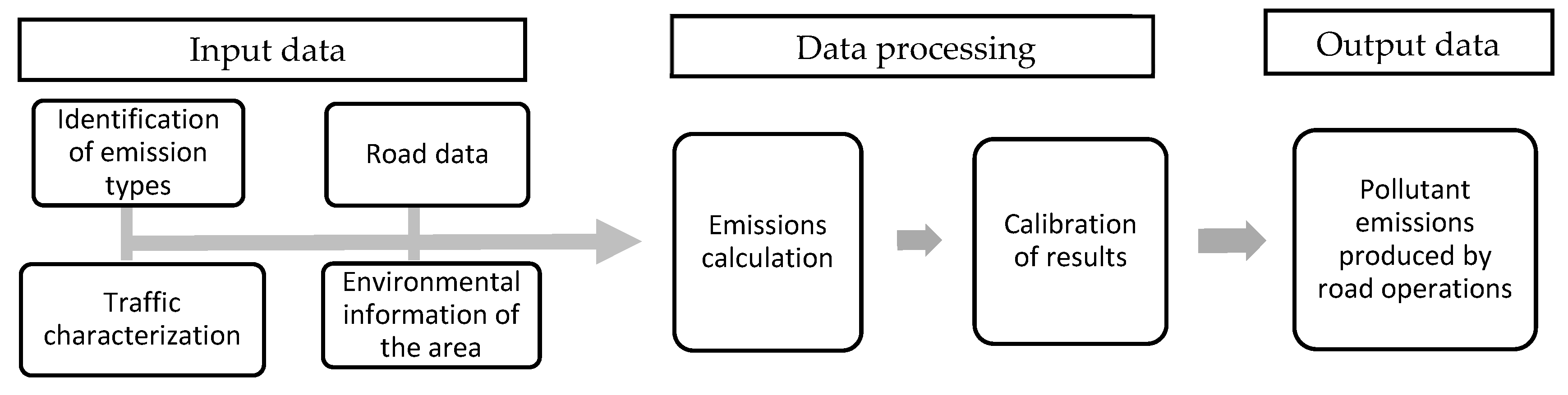
It is worth noting that for the purposes of this research, HDM-4 software has been chosen as the calculation tool, as its application has been successful in over 100 countries, both developed and developing, and provides results for each generated chemical sub-stance. On the other hand, the HDM-4 SEE (social and environmental effects) module works according to the formulas established by [10]. The formulation of emission models in HDM-4 is based on vehicle-specific fuel consumption, and fuel consumption is dependent on the vehicle characteristics, speed, and road conditions.
In this regard, Figure 3 outlines the methodological approach for quantifying emissions from road operations.

3.1. Input Data

Based on the above, the minimum input variables necessary to be introduced into the calculation tool are as follows:
  • Identification of emission types.
  • Traffic volume on the road section, refers to the annual traffic volume in each flow period, i.e., vehicles per year.
  • Vehicle speeds, operational speed of vehicles when traveling on the road.
  • Fuel consumption, pertaining to the instantaneous fuel consumption of each vehicle type, in each traffic intensity period.
  • Vehicle lifespan and model parameters.
  • Characteristics of the road section, such as section length, slopes, and road surface.
  • Maximum and minimum temperatures of the study area.
Through a literature review, it was possible to identify the types of pollutant emissions generated by vehicles in road operations. It is important to note that the case study is located in Mexico, a developing country. Consequently, there are challenges in obtaining data for the necessary variables to create a traditional inventory. In this context, to conduct this research, aside from exploring various databases, fieldwork was essential to gather and verify statistical data about vehicles using the road and existing geometric data. The consulted databases included traffic data from the Ministry of Infrastructure, Communications, and Transportation (Secretaria de Infraestructura, Comunicaciones y Transportes, SICT, Mexico City, Mexico) [77] and data from the Public Trust for Road Funds and Investment Administration of the Centinela-Rumorosa Highway Section (Fideicomiso Público de Administración de Fondos e Inversión del Tramo Carretero Centinela-Rumorosa, FIARUM, Mexicali, Mexico) [78], as well as environmental information data from the Ministry of Environment and Natural Resources (SEMARNAT, Mexico City, Mexico) [79].
Traffic composition is defined as the proportions of different types of vehicles using the road [80]. To obtain the annual average daily traffic and vehicle characterization, the configuration scheme of the main vehicles circulating on the national network published in the Mexican official standard by the SICT was used [81] (Table 1).
The first inputted data pertain to traffic and vehicle composition. This information was taken from the year 2018 as a complete count was available for this period and to avoid biased data due to the reduction in traffic in subsequent years caused by the COVID-19 pandemic. Additionally, it is important to mention that these data correspond to the typical highway traffic. On the other hand, it should be noted that the case study has specific characteristics along its route. Therefore, the segment was divided into three subsections. The first segment, from kilometers 0 to 18, is located in an urban area. The second subsection is situated around the Laguna Salada, spanning kilometers 18 to 42, characterized by a non-urban environment with a completely flat and straight terrain. The third subsection covers the range from kilometer 42 to 64, as it traverses a mountainous area with a series of curves and significant slopes. Furthermore, the entire route has two separate lanes of traffic. In this context, Table 2 presents the average annual daily traffic for both lanes, categorized within the three subsections.
In addition to the above, Table 3 shows the vehicular classification of the road section; it is noteworthy that the highest traffic is recorded in the urban area. Vehicles of type A2 (light vehicles) account for 75% on uphill and 73% on downhill.
In the same way, Table 4 displays the vehicle classification for the section located at Laguna Salada from kilometer 18 to 42. It is worth noting that this is no longer an urban area, but it does have recreational areas. The most prevalent vehicle with the highest traffic is the A2 light vehicle, accounting for 72% on the uphill and 70% on the downhill.
Table 5 presents the vehicle classification for the section located in the mountainous area from kilometers 42 to 64. This section represents lower traffic. Nevertheless, it accounts for a daily circulation of four thousand vehicles, with 65% being light vehicles on the uphill and 68% on the downhill.
With HDM-4 software, in addition to traffic and its characterization, vehicle information is inputted, including operating speeds, types of fuel used, and specific vehicle characteristics. As established previously, the emission models in HDM-4 are based on vehicle-specific fuel consumption; additionally, fuel consumption is dependent on vehicle characteristics, speed, and road conditions [82]. A travelling vehicle is associated with two types of speeds, namely the vehicle free speed and operating speed; free speed can be achieved on an uncongested road, and this is predicted using mechanistic models, and operating speed includes uphill speed, downhill speed, and the average round trip speed [83]. The equations for estimating this are described in [84].
The characterization of the vehicles and consumption and operating expenses were obtained from [85]. In order to calibrate the data related to the speed of the vehicles, a point speed study on the highway was carried out considering the methodology described in [86]. With this methodology, it is possible to obtain a representative sample of the vehicles that travel at a given point, as well as its speed characteristics under prevailing conditions of traffic and weather conditions at the time of carrying out the study, allowing speeds by user groups to be obtained. It is based on obtaining the arithmetic mean of the point speeds of the vehicles passing through a specific point. That is, a distribution of point velocities is obtained and, with it, the observed and accumulated frequency distribution. Finally, the standard deviation, the standard error of the means, and a reliability level of 95.5% are taken into account. To validate the results of the point speed study, data from the Ministry of Communications and Transportation of Mexico were used [87]. The speeds considered in the present study are presented in Table 6.
As detailed previously, road conditions affect the generation of polluting emissions. since they are closely linked to the operating speed and therefore to fuel consumption, mostly geometric features, such as distances, widths, and slopes, as well as climatic conditions of the area and road pavement deterioration in form of the roughness index (IRI).
For the geometric conditions, the conventional criterion is based on the use of project standards, which dimension the components of the road, separately and together, to achieve an adequate balance between the desirable attributes. It is worth mentioning that the downhill section was a two-lane highway before the uphill section was built since 2000, so the downhill section design has inconsistencies and is inappropriate for use in the present days. Meanwhile, the rest of the highway is made up of flat and straight sections. The case study has 81 horizontal curves on the uphill and 82 on the downhill. For this research, the data obtained by [17] of the horizontal and vertical alignments were used.
The IRI refers to an indicator that directly represents the functional condition of a pavement, and at the same time, it constitutes a complementary indicator to divide the road network according to its structural capacity. For this study, a measurement of performance indicators was carried out, including the IRI. The data collected, as well as deterioration information, are classified according to the criteria established by ASHTOO to measure the pavement surface condition. For IRI Roughness (m/km), New = 0–2, Good = 2–4, Fair =. 4–6, Poor = 6–8, and Bad ≥8. Highway pavement conditions are shown in Figure 4. It is important to mention that the analysis of the conditions was carried out based on a calculation per km. However, it is averaged for a better appreciation of the conditions of each section of the highway.
One aspect that characterizes the highway is the variability of climatic conditions and environmental conditions (Figure 5). The “Eastern” part of the road is located in the municipality of Mexicali, and it has a very dry desert climate (BWh). The maximum temperatures recorded exceed 54 degrees Celsius, while the minimum temperatures drop −7 degrees Celsius. In the central and flat area corresponding to the Laguna Salada section, a very dry semi-warm climate occurs (BWh), while in the mountainous area of the section that is located within the municipality of Tecate in the town of La Rumorosa, there is a cold desert climate (BWks) where they reach minimum temperatures of −10 degrees Celsius in winter and temperatures maximums of up to 40.3 degrees Celsius in summer. Additionally, in said area, in the rainy season, there are considerable snowfalls. For this study, data from the National Institute of Statistics and Geography of Mexico were used, as well as information from the climatological stations of the National Water Commission [79,88].
Criterion contaminant data used in this investigation were obtained from historical records and were available at air quality monitoring stations. Databases originate from stations in the United States of America and Mexico. The World Air Quality Project [89] has stations near the case study for which records date from 2008 to date. Stations closest to the case study are those of Otay Mesa Donovan Correctional Facility and Calexico-Ethel Street. On the other hand, in Mexico, the air quality monitoring stations belong to the National Air Quality Information System (SINAICA) [90]; of the three nearby stations of this network, the so-called COBACH is on the periphery the urban city and shows data closer to the traffic conditions and interurban emissions that are perceived on road sections, such as the highway. There are no air quality monitoring stations directly in the case study, so the data used correspond to these stations. The reliability between the data from the air quality monitoring stations was contrasted, finding that the variation in the records of criterion pollutants between stations does not exceed 5%.

3.2. Data Processing

Subsequently, once the input data are obtained, the model proposed by [91] is applied. This model predicts vehicle exhaust emissions based on the fuel consumption and speed. Similarly, fuel consumption is influenced by vehicle speed, which in turn depends on road characteristics and the vehicle itself. This approach allows for the analysis of changes in emission levels as a result of implementing various road maintenance and improvement strategies or when significant changes occur in the vehicle fleet on the road network [82]. On the other hand, the coefficients and constants mentioned in the formulas are derived from various studies under controlled conditions, which have enabled the creation of tables with recommended values for use in the model [1].
During the data processing, an adjustment of the Calibration Factors of Equations (1)–(7) was carried out, which by default in HDM-4 is equal to 1. However, it is important to mention that this calibration was performed only on the calibration factor k0, which responds to the calibration factor for a given emission. This adjustment consists of a relationship between the criterion pollutant value reported by the air quality monitoring station and the maximum value allowed by the reference standard, and in the present investigation, these were the Official Mexican Standards: NOM-020-SSA1-2014 [92], NOM-022-SSA1-2019 [93], NOM-021-SSA1-2021 [94], NOM-023-SSA1-2021 [95], NOM-025-SSA1-2021 [96], NOM-026-SSA1-2021 [97]. An example is the case of the calibration factor for NOM-021-SSA1-2021 is presented, which establishes a maximum hourly concentration of carbon monoxide (CO) of 26 ppm in the standard and 21 ppm, which was recorded at the monitoring stations, and the ratio of 21 ppm/26 ppm is equal to 0.8076; this value replaces the calibration factor k0 = 1.0 that was predefined in HDM4, and in this way, the information on criterion contaminants from the monitoring stations to be considered to calibrate parameters in the equations is indicated in HDM4.
This study was conducted with level 1 and 2 calibrations. This includes a desk study based on data collected from secondary sources, such as publications from government agencies and reports from previous studies, and also direct measurements of local conditions to verify and adjust the prediction capacity of the model, mainly in determining local conditions, such as traffic characterization, speeds, geometry, pavement conditions, weather, and air quality monitoring. Level 3 is outside the scope of this study as it involves significant field studies and historic real-time data, so they were not possible at this stage.
Next, the equations applied for calculating the various emissions produced by road operations are presented.
Hydrocarbons (HC)
EHC   = 3.6 k e h c 0 a 0 + a 1 k e h c 1 I F C 1 + 0.5 a 2 L I F E 10 3   S P E E D
where:
EHC: Hydrocarbon Emissions (g/veh-km)
IFC: Instantaneous Fuel Consumption (mL/s)
LIFE: Vehicle Lifetime (years)
SPEED: Vehicle Speed (km/h)
A0 a A2: Model Parameters
Kehc0: Calibration Factor (predefined = 1.0)
Kehc1: Calibration Factor (predefined = 1.0)
Carbon Monoxide (CO)
ECO   = 3.6 k e c 0 a 0 + a 1 k e c 1 I F C 1 + 0.5 a 2 L I F E 10 3   S P E E D
where:
ECO: Carbon Monoxide Emissions (g/veh-km)
IFC: Instantaneous Fuel Consumption (mL/s)
LIFE: Vehicle Lifetime (years)
SPEED: Vehicle Speed (km/h)
A0, A1, A2: Model Parameters
Kec0: Calibration Factor (predefined = 1.0)
Kec1: Calibration Factor (predefined = 1.0)
Nitrogen Oxide (NOx)
ENOX   = 3.6 k e n o x 0 a 0 + a 1 k e n o x 1 I F C 1 + 0.5 a 2 L I F E 10 3   S P E E D
where:
ENOX: Nitrogen Oxide Emissions (g/veh-km)
IFC: Instantaneous Fuel Consumption (mL/s)
LIFE: Vehicle Lifetime (years)
SPEED: Vehicle Speed (km/h)
A0 a A2: Model Parameters
Kenox0: Calibration Factor (predefined = 1.0)
Kenox1: Calibration Factor (predefined = 1.0)
Sulfur Dioxide
ESO 2 = 3.6 K e s o 0 a 0 a 1 I F C 10 3 S P E E D
where:
ESO2: Sulfur Dioxide Emissions (g/veh-km)
IFC: Instantaneous Fuel Consumption (mL/s)
SPEED: Vehicle Speed (km/h)
A0, A1: Model Parameters
Keso0: Calibration Factor (predefined = 1.0)
Carbon Dioxide (CO2)
ECO 2 = 3.6 K e c o 0 a 0 I F C 10 3 S P E E D
where:
ECO2: Carbon Dioxide Emissions (g/veh-km)
IFC: Instantaneous Fuel Consumption (mL/s)
SPEED: Vehicle Speed (km/h)
A0: Model Parameters
Keco0: Calibration Factor (predefined = 1.0)
Particulate Matter (PM)
E P M = 3.6 K e p a r 0 a 0 + a 1 k e p a r 1 I F C 10 3 S P E E D
where:
EPM: Particulate Matter Emissions (g/veh-km)
IFC: Instantaneous Fuel Consumption (mL/s)
SPEED: Vehicle Speed (km/h)
A0, A1: Model Parameters
Kepar0: Calibration Factor (predefined = 1.0)
Kepar1: Calibration Factor (predefined = 1.0)
Lead (PB)
EPB = 3.6 K e p b 0 a 0 a 1 I F C 10 3 S P E E D
where:
EPB: Lead Emissions (g/veh-km)
A0, A1: Model Parameters
Kepb0: Calibration Factor (predefined = 1.0)
On the other hand, to obtain the results, it is necessary to apply the basic equation used to estimate emissions from motor vehicles, which involves vehicle activity data and an emission factor, where the factor is provided by the aforementioned models [10].
Ep = (KRV) (FEp)
where:
Ep = Total emissions of pollutant p (Ton)
KRV = Kilometers traveled by the vehicle
FEp = Emission factor of pollutant p
The data used, as well as the data obtained from the calculation tool, are applied to the basic equation. However, because the software provides results per thousand vehicles, the emission generated by each vehicle is calculated using the following equation:
EV = HDM 4   results 1000
where:
EV = Emissions per vehicle
HDM-4 results = Outputs of SW HDM-4
Finally, with the results obtained from the calculation tool, it is necessary to adjust for the case study. To do this, the average annual daily traffic is obtained, along with its classification and the total distance of the road section under analysis. Thus, the following equation is derived:
TEOC = ( ( AADT ) ( CLV ) )   ( EV )   ( D )
where:
TEOC = Total emissions from road operation (Ton)
AADT = Average annual daily traffic
CLV = Vehicle classification
EV = Emissions per vehicle
D = Distance in kilometers

4. Results and Discussions

Finally, by applying the equations of the calculation tool and calibrating the results using Equations (8)–(10), the pollutant emissions generated by the operation of the Centinela-La Rumorosa road, spanning 64 km, are obtained. Table 7 illustrates that 372.5 tons of pollutant emissions are produced annually. Among these, 82.3% is CO2, and 2.7% is CO, together accounting for a total of 85% of the overall emissions. The second most prominent pollutant in terms of emissions is lead, constituting 13.36%. Subsequently, NOx contributes 1.2%, hydrocarbons 0.4%, PM particles 0.03%, and SO2 0.01%.
This research presents an estimation of the quantity of pollutant emissions generated by vehicles circulating on roads. Consequently, an analysis was conducted on CO2, CO, HC, NOx, PM, SO2, and Pb emitted through vehicle combustion in the case study. The findings reveal that the highest amount of generated pollutant emissions is CO2, with 306.4 annual tons, making it the most prominent, which aligns with the literature review conducted. Furthermore, the results also correspond to the understanding that the emission factor for suspended particulates from heavy vehicles is greater than the emission factor for light vehicles [98]. In this context, the section with fewer heavy vehicles generates a smaller quantity of particulates.
The case study has the particularity of encompassing three distinct characteristics: urban area (18 km), flat terrain area (24 km), and mountainous terrain area (22 km). As a result, traffic and its classification align with these characteristics. In this regard, Table 3, Table 4 and Table 5 reveal that the urban area exhibits the highest traffic (39.88%) with a greater percentage of light vehicles. Subsequently, within the flat terrain area, the highest percentage of light vehicles prevails, albeit with a lower traffic percentage than in the urban area (35.06%). Lastly, in the mountainous area, both traffic (25.06%) and the quantity of light vehicles decrease, while the number of heavy vehicles increases. Despite the aforementioned, the number of emissions generated per section does not correspond solely to the traffic volume or the length of the sections. For instance, the flat terrain section, while having the most kilometers, does not possess the highest traffic volume but generates 40.84% of emissions. This is followed by the urban segment, contributing 32.18% of emissions, even though it has the highest traffic but the lowest length. Lastly, the mountainous section, with the lowest vehicle count but a longer length than the urban segment, generates 26.98% of emissions. From the results obtained, it is possible to carry out an analysis of the data to understand the behavior of the polluting emissions that are generated by the operation of vehicles on roads, as well as their relationship with the input variables of the model. Table 8 presents a breakdown of CO2 emissions.
According to the results obtained, taking CO2 as a reference, variations in the number of emissions are identified concerning the characteristics of each of the sections of the road. In the first instance, the section of the road that generates the highest polluting emissions in the year is the one that corresponds to the Laguna Salada section. The above is mainly associated with the fact that it is the longest section, and it concentrates on the second section with the greatest AADT and truck traffic, as well as the hottest climatic zone. However, it is important to highlight that the section that generates the greatest number of polluting emissions per vehicle type is the mountainous area of the highway. This section concentrates greater slopes and degrees of curvature in its geometry, in addition to the greatest concentration of truck vehicles. The results described above allow us to understand the behavior of the different variables and their effect on the reduction or increase in emissions. However, a sensitivity analysis of road and traffic conditions is proposed for subsequent studies.
On the other hand, a limitation of this study is that k1 factor calibration that is predefined is used, because this calibration involves field studies with a direct measurement of the various characteristics of the vehicles since this factor is closely linked to the IFC for future research desirable to perform these measurements. Another limitation is that it analyzes vehicle emissions entirely during their operation, that is, while being in constant circulation. However, other circumstances can cause pollutant emissions on a road, such as toll booths, vehicle inspections, accidents, or road maintenance work, which are not considered in this analysis. These aspects are proposed as future work, promoting comprehensive emissions models.
In a general sense, this research provides an initial approach for quantifying pollutant emissions specifically along road sections in Baja California. However, this initial endeavor should be complemented by solutions or mitigation plans aimed at reducing the number of emissions produced on roads.

5. Concluding Remarks

The importance of good air quality lies in providing a healthy environment that enhances the quality of life. However, achieving this requires the commitment and participation of everyone involved. Firstly, as users, we must be aware of the environmental re-percussions of unsustainable mobility. Additionally, the entities responsible for road ad-ministration hold the responsibility of implementing the necessary measures to ensure compliance with significant environmental management tools, such as ambient quality standards, maximum permissible limits, and action plans. Therefore, it is deemed essential that in the future, regular environmental assessments and mitigation proposals should be established for the pollutant emissions generated by transportation.
The transportation sector is one of the main sources of pollutant emissions. In this regard, it is important to generate research that contributes to this topic. At a research level, there are few studies focused on polluting emissions on interurban roads, most of them focus on urban areas due to the proximity of people to these emissions. However, on roads, pollutant emissions are generated in the same way that are not near people. Nevertheless, these emissions accumulate in the atmosphere, contributing to various environmental issues, such as the greenhouse effect and global warming, affecting the biodiversity in the vicinity of the road. Also, the wind can take this emission to urban and rural zones.
Hence, this work presents a quantitative analysis of emissions generated by the operation of a road section, specifically with a case study in a developing country. However, this road has an approximate daily average of five thousand vehicles and is the only land communication route between the states of Baja California and Baja California Sur with the rest of the country, reflecting a high vehicular flow. Despite this, there are no studies or analyses of the polluting emissions generated by the operation of this road, and consequently, there are no mitigation plans for this problem.
On the other hand, it is established that the calculation tool used allows for obtaining results with the available information in a developing country, such as Mexico. Currently, the SICT is responsible for collecting traffic data from all the roads in the country. Therefore, it is possible to replicate this methodology with any road.
The results generally coincide with the literature, the predominant emissions are CO2, and having a consistent geometric design allows for lower atmospheric emissions. The agencies in charge of road management must work together with environmental agencies to have monitoring stations that allow data to be collected to better validate existing emissions models, which will allow more mitigation proposals to be made more efficient. In this regard, the results provide valuable insights for environmental researchers and could serve as a basis for new considerations in the environmental analysis on highways. This research demonstrates that it is possible to quantify emissions even in developing countries with limited databases available for such applications.

Author Contributions

The authors confirm their contributions to the paper as follows: study conception and design: all authors; data collection: all authors; analysis and interpretation of results: M.M.-A. and Á.C.; draft manuscript preparation: J.C.-R. and J.M.G.-M.; study supervision: all authors. All authors have read and agreed to the published version of the manuscript.

Funding

This research received no external funding.

Institutional Review Board Statement

Not applicable for that and for the informed consent statement.

Informed Consent Statement

Informed consent was obtained from all subjects involved in the study.

Data Availability Statement

The annual average daily traffic database can be found at https://www.sct.gob.mx/carreteras/direccion-general-de-servicios-tecnicos/datos-viales/ (accessed on 6 September 2023).

Conflicts of Interest

The authors declare no conflicts of interest.

References

  1. Torras, S.; Téllez, R.; Mendoza, J. Análisis Paramétrico del Submodelo Efectos Ambientales del HDM-4. Secretaría de Comunicaciones y Transportes (SCT) e Instituto Mexicano del Transporte (IMT). 2005. Available online: https://www.imt.mx/archivos/Publicaciones/PublicacionTecnica/pt266.pdf (accessed on 15 May 2023).
  2. Román-Hilario, N. Emisiones Contaminantes de Vehículos del Distrito de Huancayo. Doctoral Tesis, Universidad Nacional Del Centro Del Perú, Huancayo, Peru, 2017. Available online: https://repositorio.uncp.edu.pe/bitstream/handle/20.500.12894/4137/Hilario%20Roman.pdf?sequence=1&isAllowed=y (accessed on 5 March 2023).
  3. EEA. European Environment Agency. 2005. Available online: https://www.eea.europa.eu (accessed on 15 May 2023).
  4. Kean, W.; Sotos, M.; Doust, M.; Schultz, S.; Marques, A.; Deng-Beck, C. Protocolo Global para Inventarios de Emisión de Gases de Efecto Invernadero a Escala Comunitaria. Estándar de Contabilidad y de Reporte Para las Ciudades. World Resources Institute, ICLEI y C40. USA. 2014. Available online: https://ghgprotocol.org/sites/default/files/2022-12/GHGP_GPC%20%28Spanish%29.pdf (accessed on 10 March 2023).
  5. Guerra, J.; Estrategia Nacional de Cambio Climático. Comisión Intersecretarial de Cambio Climático. 2013. Available online: https://www.dof.gob.mx/nota_detalle.php?codigo=5301093&fecha=03/06/2013#gsc.tab=0 (accessed on 10 March 2023).
  6. Mendoza-Sánchez, J.F.; López-Domínguez, M.G.; González-Moreno, J.O.; Téllez-Gutiérrez, R.; Inventario de Emisiones en Carreteras Federales del Estado de Querétaro. Instituto Mexicano del Transporte. 2011. Issue 339, Volume 1. Available online: https://www.imt.mx/archivos/publicaciones/publicaciontecnica/pt339.pdf (accessed on 1 June 2023).
  7. Respira México. Retrieved. 2023. Available online: http://respiramexico.org.mx/por-que-respira-mexico/ (accessed on 9 March 2023).
  8. OMS. Organización Mundial de la Salud. 2023. Available online: https://www.who.int/es/data (accessed on 5 May 2023).
  9. Dick, H.; Gasca, J.; González, U.; Guzmán, F. Opciones Para Mitigar las Emisiones de Gases Efecto Invernadero del Sector Transportes; Compendio Cambio Climático, Una visión desde México, Instituto Nacional de Ecología: México, México, 2004. [Google Scholar]
  10. Herrera-Murillo, J.; Rodríguez-Román, S.; Rojas-Marín, J.F. Determinación de las emisiones de contaminantes del aire generadas por fuentes móviles en carreteras de Costa Rica. Rev. Tecnol. Marcha 2012, 25, 54. [Google Scholar] [CrossRef]
  11. Wichmann, E.; Peters, A. Epidemiological evidence on the effects of ultrafine particle exposure. Philos. Trans. R. Soc. Lond. Ser. A 2000, 358, 2751–2769. [Google Scholar] [CrossRef]
  12. World Health Organization; Regional Office for Europe. Health Aspects of Air Pollution with Particulate Matter, Ozone and Nitrogen Dioxide: Report on a WHO Working Group, Bonn, Germany, 13–15 January 2003; WHO Regional Office for Europe: Copenhagen, Denmark, 2003. Available online: https://apps.who.int/iris/handle/10665/107478 (accessed on 2 June 2023).
  13. Lara, C.; Mendoza, J.; López, M.; Téllez, R.; Martínez, W.; Alonso, E. Propuesta Metodológica para la Estimación de Emisiones Vehiculares en Ciudades de la República Mexicana. Secretaría de Comunicaciones y Transporte (SCT)—Instituto Mexicano del Transporte (IMT). 2009. Available online: https://imt.mx/archivos/Publicaciones/PublicacionTecnica/pt322.pdf (accessed on 20 May 2023).
  14. INECC. Estudio de Emisiones y Actividad Vehicular en Baja California; Instituto Nacional de Ecología y Cambio Climático y Secretaría de Medio Ambiente y Recursos Naturales: México, Mexico, 2011. Available online: https://www.gob.mx/inecc/documentos/2011_cgcsa_rsd_baja-california (accessed on 5 March 2023).
  15. Calderón-Ramírez, J.; Lomelí-Banda, M.; Mungaray-Moctezuma, A.; Hallack-Alegría, M.; García-Gómez, L. Efectos de CO en la población de las inmediaciones de los cruces fronterizos de México y Estados Unidos. Caso de estudio: Baja California-California. ACE Arquit. Ciudad Y Entorno 2017, 12, 29–44. [Google Scholar] [CrossRef]
  16. Liu, N.; Wang, Y.; Bai, Q.; Liu, Y.; Wang, P.; Xue, S.; Yu, Q.; Li, Q. Road life-cycle carbon dioxide emissions and emisión reduction technologies: A review. J. Traffic Transp. Eng. 2022, 9, 532–555. [Google Scholar] [CrossRef]
  17. Montoya-Alcaraz, M.; Mungaray-Moctezuma, A.; Calderón-Ramírez, J.; García, L.; Martínez-Lazcano, C. Road safety analysis of high-risk roads: Case study in Baja California, México. Safety 2020, 6, 45. [Google Scholar] [CrossRef]
  18. Navalpotro, J.A.S.; Pérez, M.S.; Becerra, A.T. Las emisiones de gases de efecto invernadero en el sector transporte por carretera. Investig. Geográficas 2011, 54, 133–169. [Google Scholar] [CrossRef]
  19. De Buen, O. Importancia de la Conservación de Carreteras. Asociación Mundial de la Carretera. 2014. Available online: https://www.piarc.org/es/pedido-de-publicacion/22252-es-Importancia%20de%20la%20conservaci%C3%B3n%20de%20carreteras (accessed on 2 June 2023).
  20. Lizárraga, C. Movilidad urbana sostenible: Un reto para las ciudades del siglo XXI. Econ. Soc. Y Territ. 2006, 22, 283–321. [Google Scholar] [CrossRef]
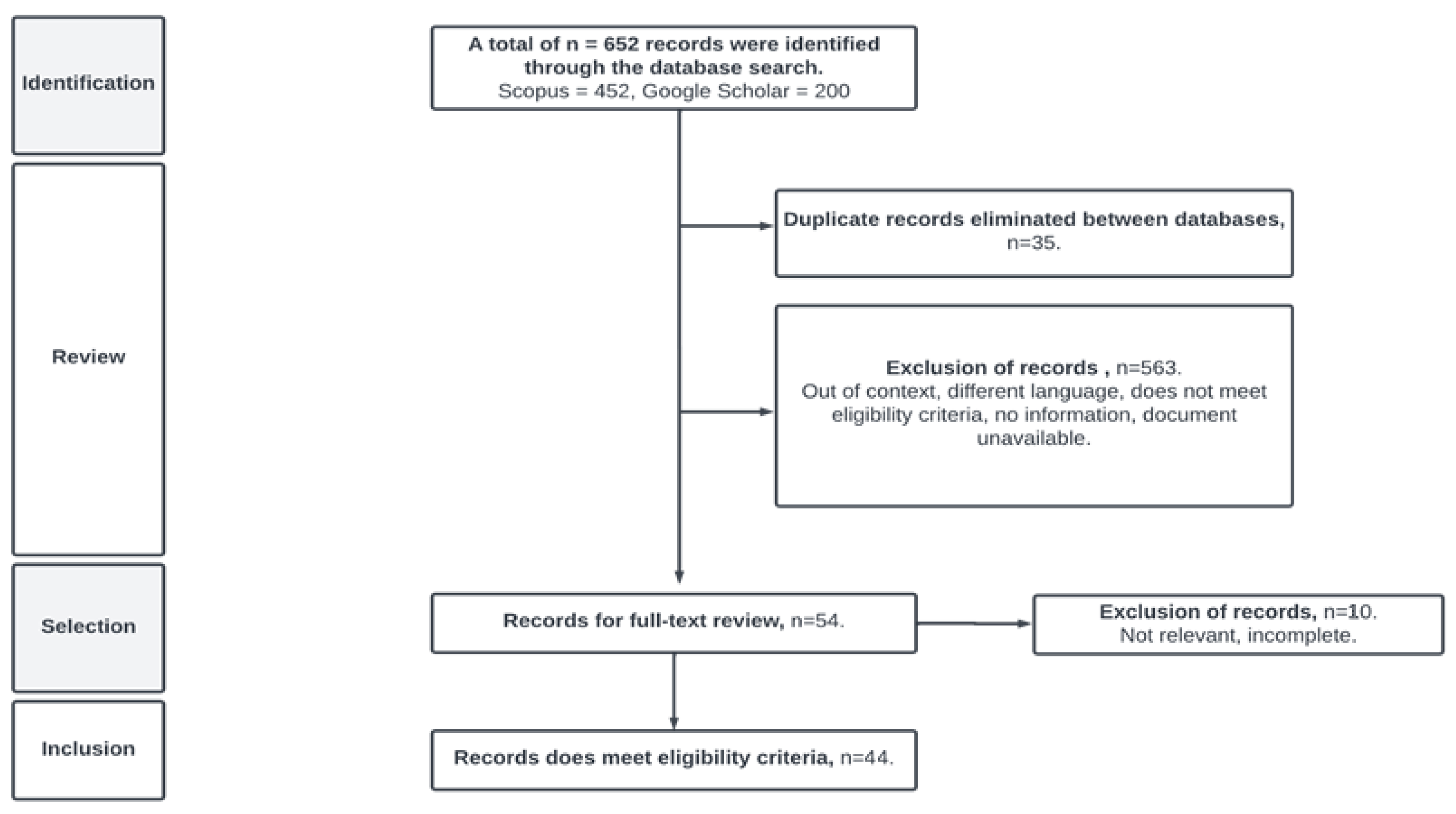
  21. Tricco, A.C.; Lillie, E.; Zarin, W.; O’Brien, K.K.; Colquhoun, H.; Levac, D.; Straus, S.E. PRISMA extension for scoping reviews (PRISMA-ScR): Checklist and explanation. Ann. Intern. Med. 2018, 169, 467–473. [Google Scholar] [CrossRef] [PubMed]
  22. Ouzzani, M.; Hammady, H.; Fedorowicz, Z.; Elmagarmid, A. Rayyan—A web and mobile app for systematic reviews. Syst. Rev. 2016, 5, 210. [Google Scholar] [CrossRef]
  23. Aromataris, E.; Fernández, R.; Godofredo, C.M.; Acebo, C.; Jalil, H.; Tungpunkom, P. Resumen de las revisiones sistemáticas: Desarrollo metodológico, realización y presentación de informes de un enfoque de revisión general. Evid. JBI Implement. 2015, 13, 132–140. [Google Scholar]
  24. Singh, S.; Kulshrestha, M.J.; Rani, N.; Kumar, K.; Sharma, C.; Aswal, D.K. An Overview of Vehicular Emission Standards. MAPAN-J. Metrol. Soc. India 2023, 38, 241–263. [Google Scholar] [CrossRef]
  25. Smit, R.; Ntziachristos, L.; Boulter, P. Validation of road vehicle and traffic emission models e A review and meta-analysis. Atmos. Environ. 2010, 44, 2943–2953. [Google Scholar] [CrossRef]
  26. Franco, V.; Kousoulidou, M.; Muntean, M.; Ntziachristos, L.; Hausberger, S.; Dilara, P. Road vehicle emission factors development: A review. Atmos. Environ. 2013, 70, 84–97. [Google Scholar] [CrossRef]
  27. Zhang, L.; Long, R.; Chen, H.; Geng, J. A review of China’s road traffic carbon emissions. J. Clean. Prod. 2019, 207, 569–581. [Google Scholar] [CrossRef]
  28. Baškovic, K.; Knez, M. A review of vehicular emission models. In Proceedings of the 10th International Conference on Logistics & Sustainable Transport, Celje, Slovenia, 13–15 June 2013. [Google Scholar]
  29. Onga, H.; Mahliaa, T.; Masjuki, H. A review on emissions and mitigation strategies for road transport in Malaysi. Renew. Sustain. Energy Rev. 2011, 15, 3516–3522. [Google Scholar] [CrossRef]
  30. McKinnon, A.; Piecyk, M. Measurement of CO2 emissions from road freight transport: A review of UK experience. Energy Policy 2009, 37, 3733–3742. [Google Scholar] [CrossRef]
  31. Alkafoury, A.; Bady, M.; Hafez, M.; Negm, A. Emissions Modeling for Road Transportation in Urban Areas: State-of-Art Review. In Proceeding of the 23rd International Conference on―Environmental Protection is a Must, Alexandria, Egypt, 11–13 May 2013. [Google Scholar]
  32. Zacharof, N.; Fontaras, G.; Ciuffo, B.; Tansini, A. An estimation of heavy-duty vehicle fleet CO2 emissions based on sampled data. Transp. Res. Part D 2021, 94, 102784. [Google Scholar] [CrossRef]
  33. Llopis, D.; Camacho, F.; Garcia, A. Analysis of the influence of geometric design consistency on vehicle CO2 emissions. Transp. Res. Part D 2019, 69, 40–50. [Google Scholar] [CrossRef]
  34. Suarez, J.; Makridis, M.; Anesiadou, A.; Komnos, D.; Ciuffo, B.; Fontaras, G. Benchmarking the driver acceleration impact on vehicle energy. Transp. Res. Part D 2022, 107, 103282. [Google Scholar] [CrossRef] [PubMed]
  35. Albores, M.; Regan, M.; Guilbeault, S.; Emisiones de Contaminantes. Comisión Para la Cooperación Ambiental. 2020. Available online: https://www.cec.org/sites/default/napp/es/pollutant-emissions.php (accessed on 23 April 2023).
  36. SEMARNAT. Guía Metodológica Para la Estimación de Emisiones Vehicular en Ciudades Mexicanas; Secretaria de Medio Ambiente y Recursos Naturales: México, Mexico, 2009.
  37. Hernández, J.; Madrigal, D.; Morales, C. Comportamiento del monóxido de carbono y el clima en la ciudad de Toluca, de 1995 a 2001. En Cienc. Ergo Sum Cienc. De La Tierra Y De La Atmósfera 2005, 11, 263–274. [Google Scholar]
  38. ENVIRA. Contaminantes Primarios y Secundarios: Estos Son Los Más Peligrosos. 2022. Available online: https://enviraiot.es/contaminantes-primarios-y-secundarios-mas-peligrosos/ (accessed on 12 March 2023).
  39. Téllez, J.; Ii, A.; Fajardo, A. Contaminación por monóxido de carbono: Un problema de salud ambiental. Rev. Salud Pública 2006, 8, 108–117. [Google Scholar] [CrossRef]
  40. Rojas, M.; Dueñas, A.; Sidorovas, L. Evaluación de la exposición al monóxido de carbono en vendedores de quioscos. Valencia, Venezuela. Rev. Panam. Salud Pública/Pan Am. J. Public Health 2001, 9, 240–244. [Google Scholar] [CrossRef]
  41. Logan, J.; Prather, M.; Wofsy, S.; Mcelroy, B. Tropospheric Chemistry: A Global Perspective. J. Geophys. Res. Ocean. 1981, 86, 7210–7254. [Google Scholar] [CrossRef]
  42. Peñaloza, N. Distribución Espacial y Temporal del Inventario de Emisiones Provenientes de las Fuentes Móviles y Fijas dela Ciudad de Bogotá D.C. Tesis de Maestría, Universidad Nacional de Colombia, Bogotá, Colombia, 2010. [Google Scholar]
  43. CORPAIRE. Corporación Para el Mejoramiento del Aire de Quito; Índice Quiteño de Calidad del Aire: Quito, Ecuador, 2004. [Google Scholar]
  44. INECC. Instituto Nacional de Ecología y Cambio Climático. Guía Metodológica para la Estimación de Emisiones Vehiculares en Ciudades Mexicanas; INECC: México, Mexico, 2007; 23p.
  45. Gómez, H.; Cuadra, M.; Alvarado, L. Instrumentos Básicos Para la Fiscalización Ambiental. Organismo de Evaluación y Fiscalización Ambiental OEFA. 2015. Available online: https://www.oefa.gob.pe/?wpfb_dl=13978.8 (accessed on 9 February 2023).
  46. Vidal, M.; Castro, J.; Morales, D. Informe Nacional de la Calidad del Aire 2013–2014; Ministerio del Ambiente MINAM: Lima, Perú, 2014. Available online: https://www.minam.gob.pe/wp-content/uploads/2016/07/Informe-Nacional-de-Calidad-del-Aire-2013-2014.pdf (accessed on 2 March 2023).
  47. Julia, C.; Fussell, J.; Franklin, M.; Green, D.; Gustafsson, M.; Harrison, R.; Hicks, W.; Kelly, F.; Kishta, F.; Miller, M.; et al. A Review of Road Traffic-Derived Non-Exhaust Particles: Emissions, Physicochemical Characteristics, Health Risks, and Mitigation Measures. Environ. Sci. Technol. 2022, 56, 6813–6835. [Google Scholar] [CrossRef]
  48. Fernández, A.; Emisiones Del Sector Transporte. Iniciativa Climática De México, ICM. 2021, p. 9. Available online: https://www.iniciativaclimatica.org/wp-content/uploads/2021/10/COP26-T9_Transporte_final.pdf (accessed on 19 February 2023).
  49. Encinas-Malagón, M.D. Medio Ambiente y Contaminación. Principios Básicos. 2011. ISBN 978-84-615-1145-7. Universidad del país Vasco, España. Available online: https://addi.ehu.es/handle/10810/16784 (accessed on 15 May 2023).
  50. Ministerio del Ambiente. Efectos de la Contaminación del Aire. Bicentenario Perú. 2021. Available online: https://infoaireperu.minam.gob.pe/efectos-de-la-contaminacion-del-aire/ (accessed on 6 January 2023).
  51. Centro Panamericano de Ingeniería Sanitaria y Ciencias del Ambiente (CEPIS) y Organización Mundial de la Salud (OMS). Curso de Orientación Para el Control de la Contaminación del Aire; Manual de Auto Instrucción: Lima, Perú, 1999.
  52. Londoño-Echeverri, C.A. Estimación de la emisión de gases de efecto invernadero en el municipio de Montería. Rev. Ing. Univ. Medellín 2006, 5, 85–96. [Google Scholar]
  53. Mukherjee, A.; McCarthy, M.; Huang, S.; Landsberg, K.; Eisinger, D. Influence of roadway emissions on near-road PM2.5: Monitoring data analysis and implications. Transp. Res. Part D 2020, 86, 102442. [Google Scholar] [CrossRef]
  54. Amirjamshidi, G.; Mostafa, T.; Misra, A.; Roorda, M. Integrated model for microsimulating vehicle emissions, pollutant dispersion and population exposure. Transp. Res. Part D 2013, 18, 16–24. [Google Scholar] [CrossRef]
  55. Mishra, R.K.; Shukla, A.; Parida, M.; Pandey, G. Urban roadside monitoring and prediction of CO, NO2 and SO2 dispersion from on-road vehicles in megacity Delhi. Transp. Res. Part D 2016, 46, 157–165. [Google Scholar] [CrossRef]
  56. Slezakova, K.; Castro, D.; Delerue-Matos, C.; Alvim-Ferraz, M.C.; Morais, S.; Pereira, M.C. Air pollution fromtraffic emissions in Oporto, Portugal: Health and environmental implications. Microchem. J. 2011, 99, 51–59. [Google Scholar] [CrossRef]
  57. Fernández-Cadete, A.; Írsula-Marén, K.; Santana-Romero, J. Behavior of Air Pollution in Industries and Its Impact on Human Health; Santiago: Santiago de Compostela, Spain, 2020; p. 152. ISSN 2227-6513. [Google Scholar]
  58. López, E.M.; Quiroz, C.M.; Cardozo, F.D.; Espinosa, A.M. Contaminación Atmosférica; Facultad Nacional de Salud Pública-Universidad de Antioquia: Medellín, Colombia, 2007. [Google Scholar]
  59. Palacios, E.E.; Espinoza, M.C. Contaminación del Aire Exterior Cuenca—Ecuador 2009–2013, Posibles Efectos en la Salud; Revista de la Facultad de Ciencias Médicas Universidad de Cuenca: Paris, France, 2014; p. 8. [Google Scholar]
  60. Adame, A. Contaminación Ambiental y Calentamiento Global; Ed. Trillas: México, Mexico, 2010; ISBN 978-607-17-0339-2. [Google Scholar]
  61. Bukola, O. Vehicle Emissions and their effects on the natural environment, a review. J. Ghana Inst. Eng. 2006, 4, 35–41. [Google Scholar]
  62. Xu, M.; Weng, Z.; Xie, Y.; Chen, B. Environment and health co-benefits of vehicle emission control policy in Hubei, China. Transp. Res. Part D 2023, 120, 103773. [Google Scholar] [CrossRef]
  63. Davoudi, M.; Barjasteh-Askari, F.; Amini, H.; Lester, D.; Mahvi, A.H.; Ghavami, V. Association of suicide with short-term exposure to air pollution at different lag times: A systematic review and meta-analysis. Sci. Total Environ. 2021, 771, 144882. [Google Scholar] [CrossRef]
  64. Urbano, P.M.; Gutiérrez, J.I.S.; Ríos, A.Y.H. Modelos de transporte por carretera y emisiones de carbono aplicables en las ciudades y su entorno. Cuadernos de Trabajo de Estudios Regionales en Economía, Población y Desarrollo 2019, 9, 3–45. [Google Scholar]
  65. Martínez, A.; Hernández, S. Catálogo de Impactos Ambientales Generados por las Carreteras y sus Medidas de Mitigación; Publicación Técnica; Instituto Mexicano del Transporte: México, México, 1999. [Google Scholar]
  66. Cohen, A.J.; Brauer, M.; Burnett, R.; Anderson, H.R.; Frostad, J.; Estep, K.; Balakrishnan, K.; Brunekreef, B.; Morawska, L.; Iii, C.A.P.; et al. Estimates and 25-year trends of the global burden of disease attributable to ambient air pollution: An analysis of data from the Global Burden of Diseases Study 2015. Lancet 2015, 389, 1907–1918. [Google Scholar] [CrossRef] [PubMed]
  67. Dünnebeil, F.; Knörr, W.; Heidt, C.; Heuer, C.; Lambrecht, U. Balancing Transport Greenhouse Gas Emissions in Cities—A Review of Practices in Germany; Transport Demand Management in Beijing, Final Report, October; Deutsche Gesellschaft für Internationale Zusammenarbeit (GIZ) GmbH and the Beijing Transportation Research Center (BTRC): Beijing, China, 2017; pp. 3–11. [Google Scholar]
  68. Mendoza, J.F.; López, M.G.; Téllez, R. Monitoreo Ambiental en Carreteras. 2010. Available online: https://www.researchgate.net/publication/344891909_MONITOREO_AMBIENTAL_EN_CARRETERAS (accessed on 13 June 2023).
  69. Odoki, J.B.; Kerali, H.G. HDM-4: Highway Development and Management. Volume Four: Analytical Framework and Model Descriptions; Asociación Mundial de Carreteras (PIARC): París, France, 2000. [Google Scholar]
  70. Prasad, C.; Swamy, A.K.; Tiwari, G. Calibration of HDM-4 Emission Models for Indian Conditions. Procedia—Soc. Behav. Sci. 2013, 104, 274–281. [Google Scholar] [CrossRef]
  71. Shrivastava, R.; Saxena, N.; Gautam, G. Air pollution due to road transportation in India: A review on assessment and reduction strategies. J. Environ. Res. Dev. 2013, 8, 69. [Google Scholar]
  72. Winkler, S.; Anderson, J.; Garza, L.; Ruona, W.; Vogt, R.; Wallington, T. Vehicle criteria pollutant (PM, NOx, CO, HCs) emissions: How low should we go? Clim. Atmos. Sci. 2018, 1, 26. [Google Scholar] [CrossRef]
  73. Torras Ortiz, S.; Friedrich, R. A modelling approach for estimating background pollutant concentrations in urban areas. Atmos. Pollut. Res. 2013, 4, 147–156. [Google Scholar] [CrossRef]
  74. Ntziachristos, L.; Samaras, Z. COPERT III Computer programme to calculate emissions from road transport. Delivery of Road Transport Emission data for EU 15 country. Eur. Environ. Agency 2000, 49, 86. [Google Scholar]
  75. Jaramillo, M.; Núñez, M.E.; Ocampo, W. Inventario de emisiones de contaminantes atmosféricos convencionales en la zona de Cali-Yumbo. Rev. Fac. De Ing. Univ. De Antioq. 2004, 31, 38–48. [Google Scholar]
  76. González, D.; Cogliati, M. Study of vehicle emissions between Neuquén and Centenario, Argentina. Atmosfera 2016, 29, 267–277. [Google Scholar] [CrossRef]
  77. SICT. Datos viales Estado de México 2018. Secretaria de Comunicaciones y Transporte. 2018. Available online: https://www.sct.gob.mx/carreteras/direccion-general-de-serviciostecnicos/datos-viales/2018/ (accessed on 10 March 2023).
  78. FIARUM. Fideicomiso Público de Administración de Fondos e Inversión del Tramo Carretero Centinela-La Rumorosa, México. 2018. Available online: https://www.bajacalifornia.gob.mx/fiarum/ (accessed on 10 March 2023).
  79. Comisión Nacional del Agua CONAGUA. Información de Estadística Climatológica. 2023. Available online: https://smn.conagua.gob.mx/es/climatologia/informacion-climatologica/informacion-estadistica-climatologica (accessed on 15 March 2023).
  80. Odoki, J.B.; Henry, G.R.; Kerali. HDM-4: Highway Development and Management. Volume Four: Analytical Framework and Model Descriptions; Asociación Mundial de Carreteras (PIARC): París, France, 2000. [Google Scholar]
  81. SICT, Norma Oficial Mexicana NOM-012-SCT-2-2017; Sobre el Peso y Dimensiones Máximas Con Los que Pueden Circular Los Vehículos de Autotransporte Que Transitan en las Vías Generales de Comunicación de Jurisdicción Federal. Norma Oficial Mexicana México, Diario Oficial de la Federación México, Distrito Federal: Ciudad de México, México, 2017.
  82. Zhang, M. Effects of road maintenance on vehicle emissions evaluating by the model of highway development and management. In Proceedings of the 4th International Conference on Sustainable Energy and Environmental Engineering, Shenzhen, China, 30–31 December 2016. [Google Scholar]
  83. Nyaga, E.W. Aerosol Remote Sensing and Modelling: Estimation of Vehicular Emission Impact on Air Pollution in Nairobi, Kenya. Doctoral Dissertation, University of Nairobi, Nairobi, Kenya, 2021. [Google Scholar]
  84. Bennett, C.R.; Greenwood, I.D. Modeling Road User and Environmental Effects in HDM-4, Version 3.0; International Study of Highway Development and Management Tools (ISOHDM); World Road Association (PIARC): Paris, France, 2003; Volume 7. [Google Scholar]
  85. Arroyo, J.; Torres, G.; González, J.; Hernández, S. Costos de Operación Base de Los Vehículos Representativos del Transporte Interurbano 2018. Instituto Mexicano del Transporte y Secretaria de Comunicaciones y Transportes. Publicación Técnica. 2018. Available online: https://imt.mx/archivos/Publicaciones/PublicacionTecnica/pt526.pdf (accessed on 13 April 2023).
  86. Cal, R.; Cárdenas, J. Ingeniería de Tránsito: Fundamentos y Aplicaciones; Alpha Editorial: Bogota, Colombia, 2018. [Google Scholar]
  87. Secretaria de Comunicaciones y Transportes. Velocidades de Punto, Adendum al Libro Datos Viales. 2020. Available online: https://www.sct.gob.mx/fileadmin/DireccionesGrales/DGST/Velocidades_de_punto/Vel-DV2020.pdf (accessed on 2 March 2023).
  88. Instituto Nacional de Estadística y Geografía. Geografía y Medio Ambiente. 2023. Available online: https://www.inegi.org.mx/temas/climatologia/ (accessed on 29 February 2024).
  89. The World Air Quality Project. Air Quality Historical Data Platform. 2023. Available online: https://aqicn.org/data-platform/register/ (accessed on 29 March 2023).
  90. SINAICA. Sistema Nacional de Información de la Calidad del Aire. 2023. Available online: https://sinaica.inecc.gob.mx/ (accessed on 15 November 2023).
  91. Hammerstrom, U. Proposal for a Vehicle Exhaust Model in HDM-4, ISOHDM Supplementary Technical Relationships Study, Draft Report; Administradora Sueca de Caminos: Borlange Sweden, 1995. [Google Scholar]
  92. NOM-020-SSA1-2014. Norma Oficial Mexicana “Valor Límite Permisible Para la Concentración de Ozono (O3) en el Aire Ambiente y Criterios Para su Evaluación”. Available online: http://diariooficial.gob.mx/nota_detalle.php?codigo=5356801&fecha=19/08/2014#gsc.tab=0 (accessed on 15 November 2023).
  93. NOM-022-SSA1-2019. Norma Oficial Mexicana “Criterio Para Evaluar la Calidad del Aire Ambiente, con Respecto al Dióxido de Azufre (SO2). Valores Normados Para la concentración de dióxido de azufre (SO2) en el Aire Ambiente”. Available online: https://www.dof.gob.mx/nota_detalle.php?codigo=5568395&fecha=20/08/2019#gsc.tab=0 (accessed on 15 November 2023).
  94. NOM-021-SSA1-2021. Norma Oficial Mexicana “Criterio Para Evaluar la Calidad del Aire Ambiente, con Respecto al Monóxido de Carbono (CO). Valores Normados Para la Concentración de Monóxido de Carbono (CO) en el Aire Ambiente”. Available online: https://dof.gob.mx/nota_detalle.php?codigo=5634084&fecha=29/10/2021#gsc.tab=0 (accessed on 15 November 2023).
  95. NOM-023-SSA1-2021. Norma Oficial Mexicana “Criterio Para Evaluar la Calidad del Aire Ambiente, con Respecto al Dióxido de Nitrógeno (NO2). Valores Normados Para la Concentración de Dióxido de Nitrógeno (NO2) en el Aire Ambiente”. Available online: https://www.dof.gob.mx/nota_detalle.php?codigo=5633854&fecha=27/10/2021#gsc.tab=0 (accessed on 15 November 2023).
  96. NOM-025-SSA1-2021. Norma Oficial Mexicana “Criterio Para Evaluar la Calidad del Aire Ambiente, con Respecto a las Partículas Suspendidas PM10 y PM2.5. Valores Normados Para la Concentración de Partículas Suspendidas PM10 y PM2.5 en el Aire Ambiente”. Available online: https://www.dof.gob.mx/nota_detalle.php?codigo=5633855&fecha=27/10/2021#gsc.tab=0 (accessed on 15 November 2023).
  97. NOM-026-SSA1-2021. Norma Oficial Mexicana “Criterio Para Evaluar la Calidad del Aire Ambiente, con Respecto al Plomo (Pb). Valor Normado Para la Concentración de Plomo (Pb) en el Aire Ambiente”. Available online: https://www.dof.gob.mx/nota_detalle.php?codigo=5634085&fecha=29/10/2021#gsc.tab=0 (accessed on 10 June 2023).
  98. Zhu, S.; Qiao, Y.; Peng, W.; Zhao, Q.; Li, Z.; Liu, X.; Wang, H.; Song, G.; Yu, L.; Shi, L. An Experimental Framework of Particulate Matter Emission Factor Development for Traffic Modeling. Atmosphere 2023, 14, 706. [Google Scholar] [CrossRef]
Figure 1. Case Study: Centinela-La Rumorosa Highway, Baja California, Mexico.
Applsci 14 02921 g001
Figure 2. PRISMA-SCR flowchart of the literature screening and selection process.
Applsci 14 02921 g002
Figure 3. Methodological approach for quantifying pollutant emissions from road operations.
Applsci 14 02921 g003
Figure 4. Highway surface conditions.
Applsci 14 02921 g004
Figure 5. Highway climatic conditions.
Applsci 14 02921 g005
Table 1. Vehicle classification (VCL) scheme.
Applsci 14 02921 i001A2Light Vehicles
Applsci 14 02921 i002A′2Pick-Ups
Applsci 14 02921 i003B22-Axle Buses
Applsci 14 02921 i004B33-Axle Buses
Applsci 14 02921 i005C22-Axle Cargo Trucks
Applsci 14 02921 i006C33-Axle Cargo Trucks
Applsci 14 02921 i007T3-S2Articulated Truck
Applsci 14 02921 i008T3-S3
Applsci 14 02921 i009T3-S2-R4
Table 2. Annual average daily traffic (AADT)).
Sectionkm from 0–18km from 18–42km from 42–64
Uphill630755134185
Downhill635856223775
Table 3. Vehicle classification for Section 0+000 al 18+000.
UphillDownhill
VCLQuantityVehicle PercentageVehicle TypeQuantityVehicle Percentage
A2473075A2464173
A′2250.4A′2641
B2631B2641
B31392.2B31342.1
C267510.7C264810.2
C31512.4C32033.2
T3-S23725.9T3-S24396.9
T3-S3761.2T3-S3761.2
T3-S2-R4761.2T3-S2-R4891.4
Total6307100Total6358100
Table 4. Vehicle classification for Section 18+000 al 42+000.
UphillDownhill
VCLQuantityVehicle PercentageVehicle TypeQuantityVehicle Percentage
A2396972A2393570
A′260.1A′2340.6
B2551B2561
B31272.3B31352.4
C24748.6C25229.3
C3721.3C3791.4
T3-S25299.6T3-S25579.9
T3-S31542.8T3-S31632.9
T3-S2-R41272.3T3-S2-R41412.5
Total5513100Total5622100
Table 5. Vehicle classification for Section 42+000 al 64+000.
UphillDownhill
VCLQuantityVehicle PercentageVehicle TypeQuantityVehicle Percentage
A2272065A2256768
A´2170.4A´280.2
B2801.9B2721.9
B31263B31133
C23979.5C23399
C3421C3340.9
T3-S255613.3T3-S245712.1
T3-S3801.9T3-S3230.6
T3-S2-R41674T3-S2-R41624.3
Total4185100Total3775100
Table 6. Point speed study results.
VCLLegal Speed (km/h)Median Speed (km/h)Max Speed (km/h)
PlainUphillDownhillPlainUphillDownhillPlainUphillDownhill
Car11080801117976158118138
Bus80606010466571338883
Trucks8060609051571338893
Table 7. Pollutant emissions generated by the operation in the case study.
Kilometers/Area
CompoundUrban Area km 0–18Laguna Salada km 18–42Mountainous Area km 42–64Totals (g)Total (Ton)
HC535,569.18620,600.50315,859.841,472,029.521.47
CO3,901,463.074,336,926.051,965,043.5310,203,432.6410.20
NOx1,392,773.901,855,356.391,243,735.034,491,865.324.49
PM27,720.0935,998.3232,220.9995,939.400.10
CO295,241,818.04124,295,181.3386,868,295.74306,405,295.11306.41
SO214,018.9819,191.1314,578.0247,788.120.05
Pb18,765,391.8620,958,666.6210,052,981.5249,777,040.0049.78
Table 8. CO2 emissions analysis.
km from 0–18km from 18–42km from 42–64
CO295,241,818.04124,295,181.3386,868,295.74
Road km364844
Emissions per km2,645,606.062,589,482.941,974,279.45
AADT12,66511,1357,960
Emissions per vehicle208.89232.55248.03
Disclaimer/Publisher’s Note: The statements, opinions and data contained in all publications are solely those of the individual author(s) and contributor(s) and not of MDPI and/or the editor(s). MDPI and/or the editor(s) disclaim responsibility for any injury to people or property resulting from any ideas, methods, instructions or products referred to in the content.

