Abstract
The deployment of megaconstellations in low Earth orbit (LEO) poses significant collision risks with space debris. This paper focuses on analyzing the short-term and long-term collision probabilities of megaconstellations to assess their collision risk. Firstly, a short-term collision risk evolution model is developed to accurately address rendezvous collisions. Secondly, a long-term collision risk evolution model is established by considering space object density, space debris attenuation, space target disintegration, and the distribution of disintegration targets. Through simulations conducted on the Starlink Phase I constellation, the results demonstrate a 30–40% increase in short-term collision probability within the constellation shell, a 70.2% probability of at least one collision during the constellation’s lifetime, and a 25.3% increase in secondary collisions following a collision event. This study provides a reference and application for analyzing the orbital safety of LEO megaconstellations and for promoting the sustainable development and utilization of space resources.
1. Introduction
The increase in human space activities is the main factor leading to the growing severity of the spacecraft safety situation. With the increasing number of satellites in space, collisions, explosions and failures may occur during long-term operation, which are often accompanied by a large number of space debris objects, resulting in a further increase in the density of space objects and further aggravating the risk of satellite collisions. If such a vicious cycle is not controlled, it may eventually produce the Kessler syndrome [1], causing the spacecraft to lose its orbital environment.
The reference [2] shows that as of 6 December 2023 there were 36,500 space debris objects greater than 10 cm in space and 1,000,000 space debris objects from 1 cm to 10 cm. The number of debris objects regularly tracked by Space Surveillance Networks and maintained in their catalog is about 35,150. These cataloged targets are distributed in orbits at various altitudes, and most of them pose no security threat to the orbit in which a low-orbit megaconstellation is located. Therefore, in order to reduce the amount of calculation and facilitate accurate and fast collision probability calculation, it is necessary to screen out targets that do not pose a security threat to the LEO megaconstellation as much as possible.
In recent years, the concept of commercial Internet satellite platforms has been proposed, resulting in a wave of megaconstellation construction. As of May 2023, Starlink had launched 4521 satellites and OneWeb had launched 636 satellites. Based on data from the International Telecommunications Union (ITU), the Federal Communications Commission (FCC), and Jonathan’s Space Pages, many companies have proposed construction plans for megaconstellations in low Earth orbit (LEO) [3]. These megaconstellations contain a large number of small satellites, and they are all in the same region, with a given width. If the deployments are completed in accordance with the plans, then the number of satellites in orbit will be several times the sum of the number of past launches. Table 1 gives some plans for megaconstellations in LEO.

Table 1.
Some plans for megaconstellations in LEO [4,5,6,7,8].
Therefore, whether from the perspective of the safety of the LEO megaconstellation itself or the sustainability of the space environment, research on the orbital safety of low-orbit megaconstellations, especially collision safety, is necessary and urgent.
The megaconstellations in LEO represented by the Starlink constellation have begun to be deployed. From 2019 to April 2023, Starlink showed frequent close proximity during the first phase of deployment. Starlink-44 had a close approach with Euro-Aeolus satellites in 2019 [9]. About 1600 close proximity events occurred in 2021, accounting for half of all the space proximity events of the year [10,11].
With the deployment of the constellation programs, the environment in LEO space is becoming increasingly problematic. Taking the OneWeb constellation as an example, Jonas et al. studied the interaction between the space debris environment and the megaconstellations [12], where the influence of LEO megaconstellations on the space environment was investigated [13,14]. Lorenzo designed a simple risk assessment statistical tool for megaconstellations in the LEO space debris environment to analyze the influence of the main parameters of the constellation on their vulnerability [15]. In addition, Isoletta proposed an uncertainty-aware Cube mid-term collision risk assessment algorithm, which is capable of evaluating the target mid-term collision frequency in low orbit [16]. Adilov et al. estimated the expected annual cost of a satellite’s collision with orbital debris based on orbital debris economics [17].
Due to the limited accuracy of the tracking data used to assess the risk of collisions, the maneuvers currently being performed far exceed the necessary level, which leads to overestimates. Campiti proposes a solution for equipping satellites with sensors that will enable them to autonomously track dangerous objects when at risk of collision and refine their location knowledge before making maneuvering decisions, enabling data collection and estimating collision risk, thereby improving the accuracy of final predictions and reducing false alarms [18].
Reference [19] introduced a dimensionless index, termed the “volumetric collision rate index”, through an analysis of the analytical equation that delineates collision rates. This index, developed based on rational simplifications and assumptions, is distinctly contingent upon the spatial density of both intact objects and cataloged fragments. While it has been utilized to assess the LEO environment, the analysis has thus far been limited to the period spanning from mid-2008 to mid-2020, lacking a more extensive exploration of subsequent evolutionary trends.
Eduardo et al. [20] formulated a statistical model that integrates the precision of colli-sion probability algorithms with the efficacy of statistical methodologies to assess the in-fluence of satellite swarms on the environment. Nonetheless, the model is built upon sev-eral assumptions, and it lacks a comprehensive long-term evolutionary analysis. Megaconstellation satellites may disintegrate and generate hundreds or thousands of space debris objects if a collision occurs due to their small mass and fast running speed. The debris generated by the collision can stay in space for a long time and may cause secondary damage to the constellations [21].
Lewis [22] introduced a large constellation to analyze the influence of low-orbit megaconstellation deployment on the collision probability of space debris. Under the condition that the postmission disposal criteria are met, the amount of space debris will continue to grow. Le May used the MASTER-2009 debris evolution model to simulate the OneWeb and SpaceX constellations, and further analyzed the influence of constellation parameters and the long-term influence of satellites that failed to perform deorbit operations [23]. Rossi utilized different tools developed by IFAC-CNR to analyze the short-term to long-term constellation influences for determining the effects associated with constellation deployment and execution [24]. For the long-term sustainable use of the space environment, many scholars have proposed debris mitigation plans for megaconstellations [25,26].
Scholars have conducted pertinent research on the safety analysis of large constellations in low Earth orbit environments. Ana S. [27] recently introduced a spatial-occupancy-based filter for satellite collision screening, employing short-term space occupancy and common orbit screening methods to address space collision challenges. Nonetheless, further enhancements and optimizations of this filter are imperative, necessitating the inclusion of additional factors and constraints to augment its reliability and effectiveness. Additionally, Zhang et al. [28] utilized orbital perturbation theory to analyze the long-term orbital evolution characteristics of Starlink satellites. The analysis included studying rendezvous scenarios between faulty and operational satellites within the same or different orbital planes, along with providing collision probabilities stemming from faulty satellites. While that study offers valuable insights for future space traffic management, its primary focus lies on the collision risks associated with satellite malfunctions, with limited consideration given to the potential impact of other factors, such as space debris, on collision risks.
However, spacecraft and space debris are mainly concentrated in the low Earth orbit region, and if the traditional two-pair analysis method is used to solve the intersection collision of the two targets, the calculation will be very large. This paper focuses on how to solve the problem quickly and accurately for rendezvous collisions, and uses a sequence of filters to greatly reduce the computational expense of the algorithm. On this basis, to evaluate the collision risk of megaconstellations (especially the Starlink constellation), a short-term collision probability calculation model and a long-term collision probability calculation model are established. These models are used to calculate the collision risks of the Starlink constellation.
The main contributions of this work can be summarized as follows: (1) A proximity analysis method for large space debris and large satellites is proposed, and a space collision target filtering method for large-scale space debris and large-scale satellites is studied. (2) A collision evolution calculation method for large-scale space debris and large-scale satellites is proposed. By filtering and partitioning data, the computing efficiency is improved while satisfying high accuracy. (3) Aiming at the long-term collision risk problem after the deployment of low-orbit megaconstellations, a long-term collision risk calculation model for low-orbit megaconstellations is established.
The paper is organized as follows: In Section 2, the calculation methods for short-term and long-term collision probabilities are presented. Based on the proposed method, the short-term and long-term collision probabilities of the Starlink constellation are calculated, as presented in Section 3. Furthermore, through comparison with the collision probability before constellation deployment, the increased collision risk percentage after constellation deployment is obtained. Finally, in Section 4, concluding remarks as well as future perspective are given.
2. Short-Term and Long-Term Collision Probability Calculation Models
2.1. Short-Term Collision Probability Calculation Model
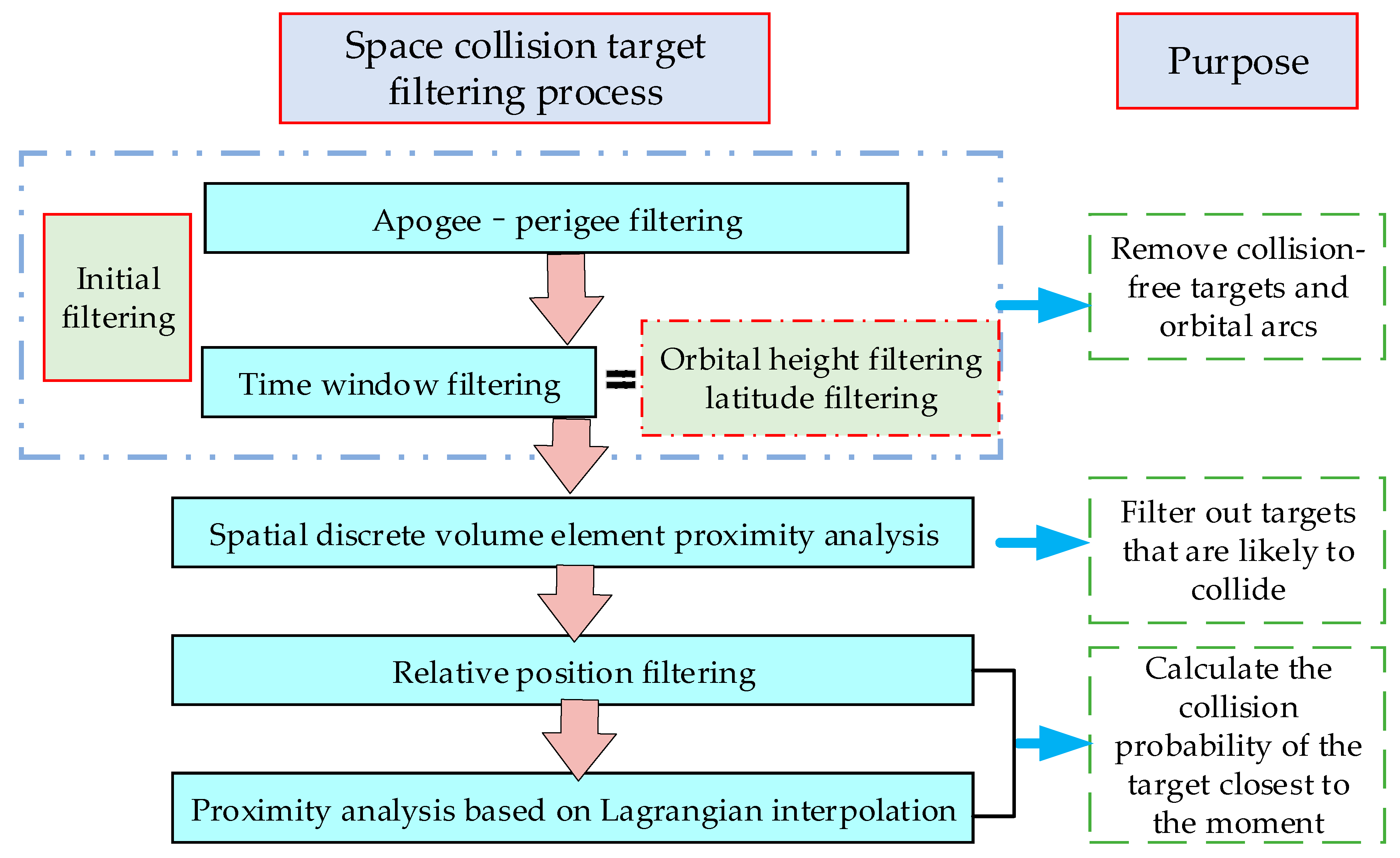
The orbital prediction model in this summary uses the SGP4 model to carry out short-term collision studies. This section establishes a proximity analysis method for large-scale space debris and large-scale satellites to eliminate the dangerous targets. The short-term collision probability computational model is constructed in accordance with the collision probability calculation method for the rendezvous target. This model is used to calculate short-term in-orbit natural evolution collisions in the shell where the constellation is located. A series of methods are used for proximity analysis of space targets, as shown in Figure 1.
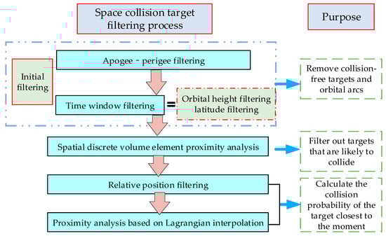
Figure 1.
Space targets proximity analysis process.
2.1.1. Apogee–Perigee Filtering
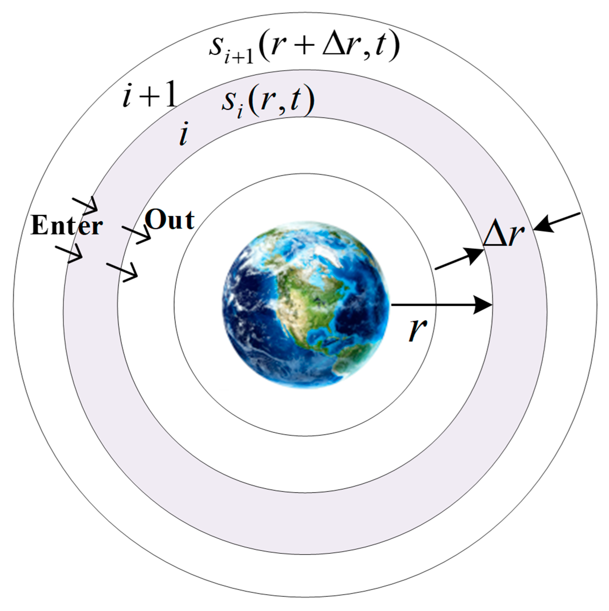
When the orbital altitude of the LEO megaconstellation is determined, the constellation satellites will operate in the constellation shell. At this time, the orbit of the space object and the shell have three states: intersection, inclusion, and separation. Space objects with orbits intersecting the shell or that are contained within the shell may collide with the constellation satellites, and space objects with orbits separated from the shell will not collide with the constellation. Therefore, the targets that may collide with the constellation shell can be preliminarily screened in accordance with the geometric relationship for the apogee and perigee of the target orbit. The relationship between the apogee–perigee and the shell of the space target is shown in Figure 2.
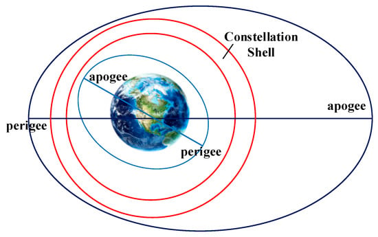
Figure 2.
Schematic of the relationship between the space target and the shell.
Assuming that the height of the constellation shell is D, the nominal orbital semi-major axis of the constellation satellites is , and the apogee and perigee of the space target are and , respectively. Given that the eccentricity of the LEO megaconstellation satellites is approximately 0, the nominal orbital radius of the constellation can be approximately equal to . As shown in Figure 2, the apogee of the space target is compared with the upper bound of the constellation shell, and the perigee of the space target is compared with the lower bound of the constellation shell. If the perigee is greater than the radius of the upper bound of the constellation shell or the apogee is smaller than the radius of the lower bound of the constellation shell, then the target is not a threat and should be eliminated. The apogee–perigee filtering method is expressed as
2.1.2. Time Window Filtering
The space targets may collide with the constellation satellite only when they travel into the shell of the constellation. Thus, the orbital altitude of the space target position determines whether it may collide with a constellation satellite. When the height of the space target position is outside the range of the shell height, the target will not collide with the constellation satellite. The constellation satellite may collide with the target only when the space target is within the shell range.
Assuming that the position and velocity of the space target at moment is , the radius of the space target at the moment is:
Given that the height interval of the constellation shell is , the time window for the possible collision between the space target and the constellation satellite can be expressed as
Different LEO megaconstellations have different orbital inclinations, and the latitude ranges that the constellations can cover are also different. Space targets may be higher than the latitudes that the constellation can cover when passing through the shell. Therefore, whether the latitude is within the latitude range covered by the constellation when the satellite is in the constellation shell should be continuously analyzed.
In accordance with the integral formula of orbital area, the moment vector of momentum per unit mass is expressed as
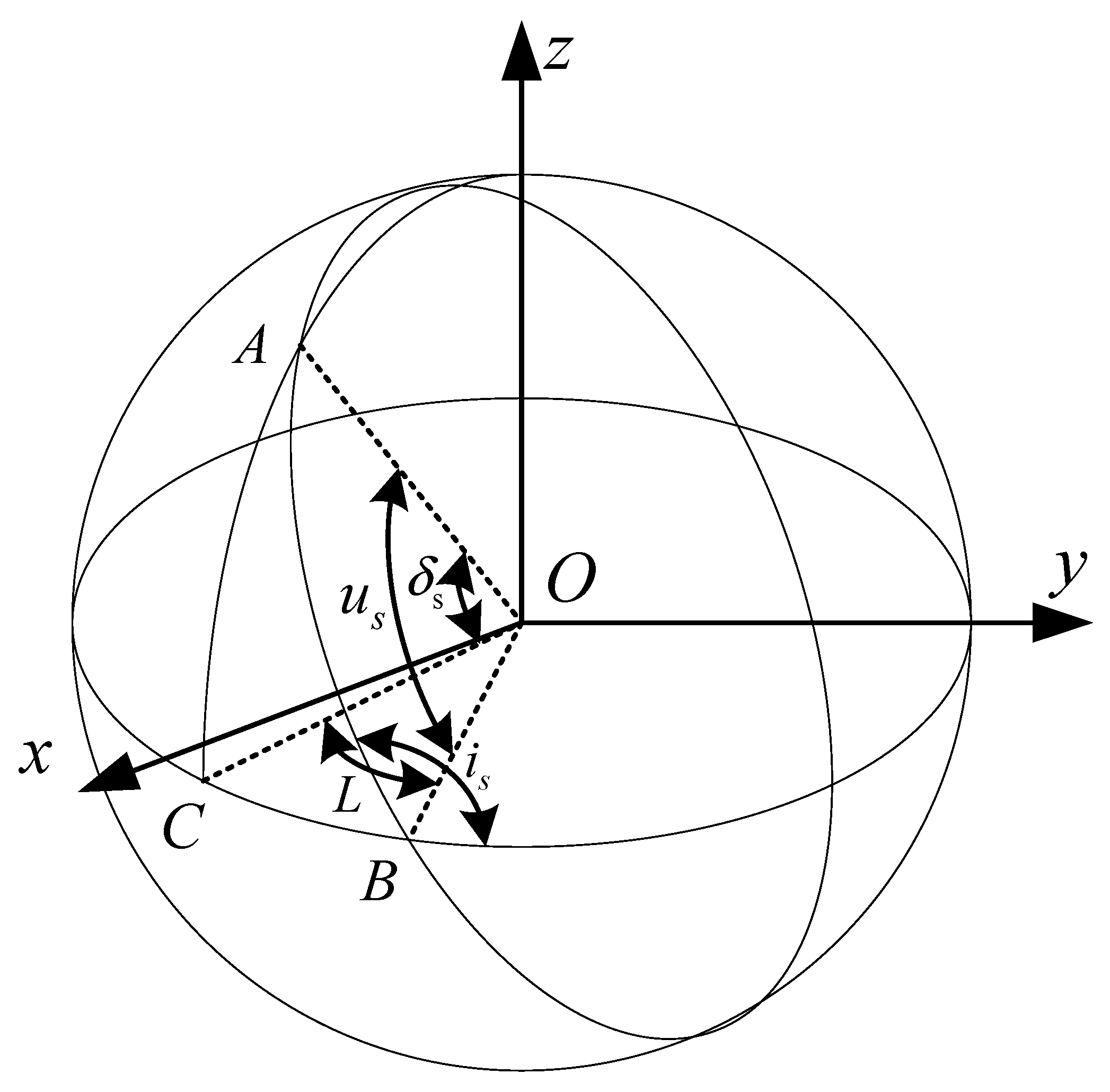
where are the projected sizes of the moment of momentum per unit mass in the directions of the three coordinate axes. Given that the orbital inclination of the space target is the angle between the momentum moment vector and the Earth’s north pole, we obtain
where is the modulus of the unit vector moment of momentum. We can obtain the positional relationship by projecting the satellite orbit on the ground, as shown in Figure 3.
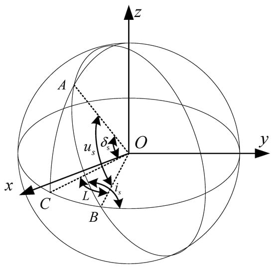
Figure 3.
Projection of the space target orbit on the ground.
In accordance with the spherical triangle, we can obtain:
where is the phase of the space target , and is the latitude of the space target . When the latitude of the space target within the window range is greater than the sum of the orbital inclination of the constellation and the offset of the orbital inclination , the space target will not collide with the constellation satellite and should be eliminated. The filtering is expressed as
2.1.3. Spatial Discrete Volume Element Proximity Analysis
The probability of collision between space targets and constellation satellites after apogee–perigee filtering and time window filtering is high. If the pairwise calculation method is used to determine whether two targets collide, then the computational complexity will vary in second-order growth with the number of constellation satellites and the number of space targets. Thus, the collision probability calculation of LEO megaconstellations is unsuitable. In this section, the constellation shell is divided into several space volume elements, and the objects that may collide are filtered by judging the distance among the space objects in each volume element. At this time, the computational complexity is in linear growth with the number of constellation satellites and the number of space objects. This condition can greatly reduce the computational complexity of collisions between LEO megaconstellations and space debris, and improve computational efficiency.
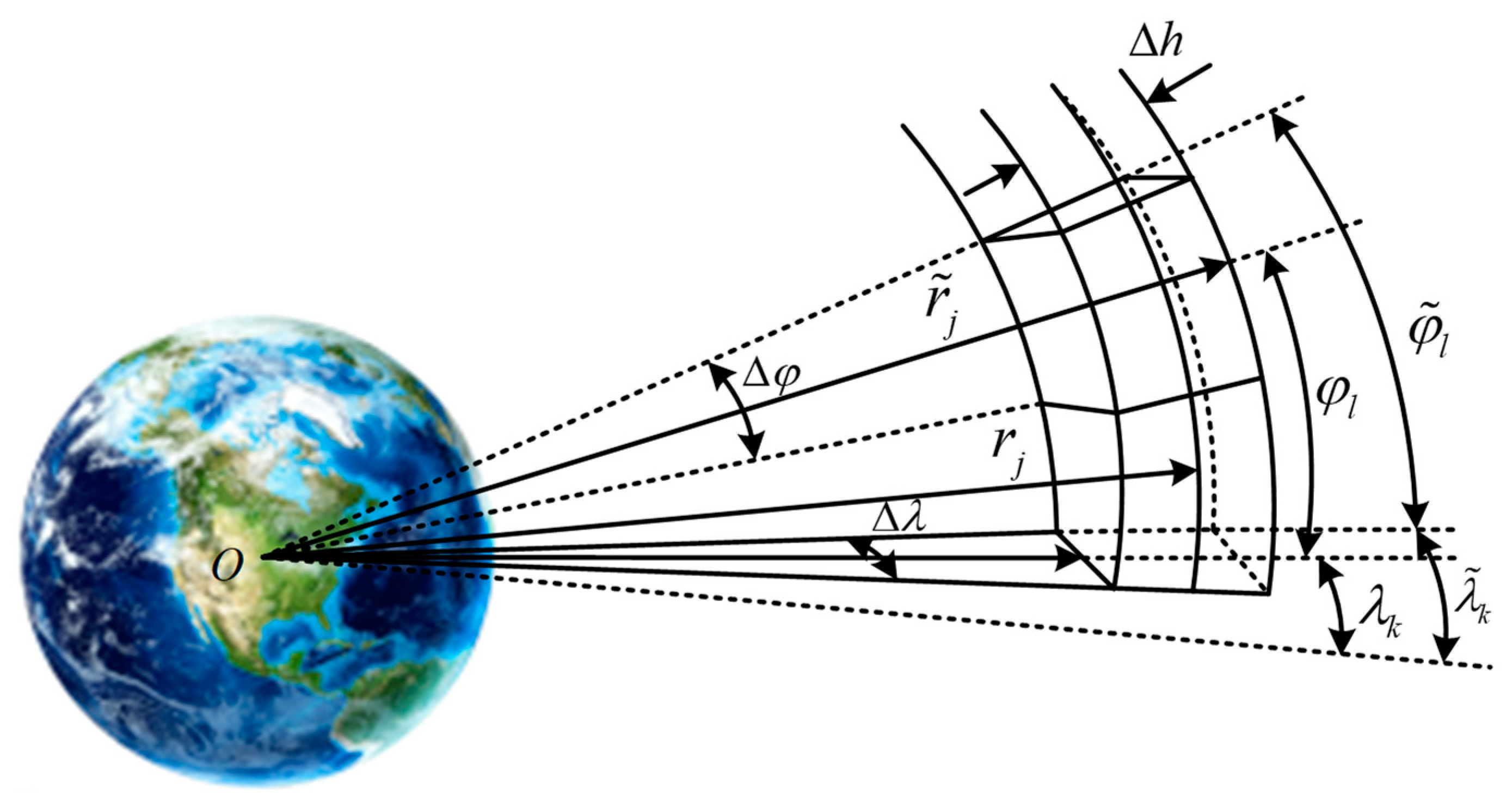
The space target orbit used in this study is defined under the J2000 inertial coordinate system, so the discrete volume element coordinate system is also defined as the J2000 inertial coordinate system. In the inertial coordinate system, the constellation shell is centered on the center of the Earth, and the spherical coordinates are established along the three directions of geocentric distance, longitude, and latitude. The discrete volume element is the starting point , and the space of the constellation shell is divided into several space volume elements in accordance with the interval . Figure 4 shows a schematic of a space volume element.
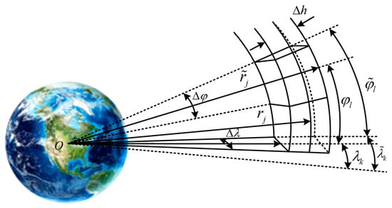
Figure 4.
Schematic of space discrete volume element.
In accordance with Figure 4, the coordinates of the space volume element in three directions are expressed as
The center of the space volume element is expressed as
The volume element division needs to consider factors such as calculation amount, storage amount, and accuracy. The larger the volume element, the less the number of traversed volume elements, the clearer the trajectory of the space target in the volume element, and the greater the number of targets appearing in the same volume element at the same time, resulting in an increase in the computational complexity of collision discrimination between targets. The smaller the discrete volume element, the fewer objects appear in the same volume element, the more time it takes to traverse the volume element, and the trajectory points of spatial objects in the volume element may be skipped, resulting in a decrease in computational accuracy. Therefore, setting the volume element size reasonably becomes the key to the approach analysis.
The orbital planes of LEO megaconstellations are uniformly distributed along the right ascension of ascending node direction, and the phase and latitude differences between satellites in the orbital plane are equal. A parameter slightly smaller than the reference standard is selected to divide the volume element while ensuring a small number of LEO megaconstellation satellites in the volume element. The volume of the volume element is increased so that the trajectory continuity of the space target in the volume element is stronger. Given that the size of volume elements decreases along the latitudinal direction, the common method is to introduce the maximum latitude and combine the volume elements with the latitude greater than that in each altitude layer into the same volume element to deal with the volume elements near the poles of the constellation shell.
2.1.4. Relative Position Filtering
When the space target is in the same volume element, it is judged whether a collision occurs between satellites by the approach distance. Given that the attitude of the space target is unknown, the space target is calculated as an envelope sphere. When the distance between the centers of mass of the two targets is less than the joint radius R, the two targets are considered to have collided immediately.
The true position of the space target has a random deviation, so the collision between the two space targets is a probabilistic event. In accordance with the “” rule, the true position of the space target has a high probability of being within three standard deviations of the average position. Therefore, we can eliminate the targets that may collide for the next calculation in accordance with the relative position of the two space targets and the “” rule.
Assuming that the position error square matrix of the two space targets in the orbital coordinate system is
the variance matrix of the relative position vectors of the two targets in the Earth inertial coordinate system is
In accordance with the “” rule, when two space targets may collide, the relative distance between the two targets satisfies the following conditions:
where and are the position vectors of the space target in the Earth inertial coordinate system. is the joint error distance in the Earth inertial coordinate system.
2.1.5. Proximity Analysis Based on Lagrangian Interpolation
Two space targets filtered out by relative positions may collide. Given that the two targets are most likely to collide when the orbits are closest, the collision probability at the closest orbit is regarded as the probability of collision between the two space targets. In reality, orbit prediction usually requires a certain step size. The step size cannot be infinitely small, and the trajectory cannot be continuous. Therefore, the predicted trajectory point is not necessarily the closest position of the orbit. Interpolation in accordance with the trajectory of the space target in the space cube must be performed to fit the curve equation of the orbit and find the position closest to the moment.
Orbits are usually fitted by using Lagrangian interpolation. Suppose the moment when the two targets in the space volume element are closest to the trajectory point is , and let the position vector of one of the space targets be . Two trajectory points are selected before and after the closest trajectory point, and five points with the closest trajectory point are used as interpolation points to perform polynomial interpolation. The constructor is obtained in accordance with the Lagrangian interpolation method.
The Lagrangian interpolation fitting curve equation of the target orbit can be obtained as:
Given that the fitting curve is a quartic polynomial and the interpolation points are known, the Lagrangian interpolation fitting curve equation can be expressed as:
In accordance with (15), the equation system of the linear curve is obtained as:
In accordance with the above formula, the expression of the space target trajectory fitting equation can be obtained. The same method can be used to obtain the space target velocity fitting equation expression . The relative distance vector of the two targets is:
The relative position vector over time can be expressed as
The relative distance is the closest moment when it reaches the minimum value, which can be expressed as
In accordance with the above formula, the closest time in the range of five trajectory points can be obtained, and the motion state of the two collision targets in space at the intersection point can be obtained by bringing into , , , and .
2.1.6. Collision Probability Calculation Model
The position error of the encounter target is transformed into the encounter coordinate system, and the probability density function of the 3D Gaussian distribution forming the joint error ellipsoid is
The joint position error ellipsoid is projected to the encounter plane, and the encounter coordinate system is rotated as the calculation coordinate system, so that the axis of the calculation coordinate system is consistent with the direction of the major semi-axis of the joint position error ellipse. The collision probability by integrating the joint position error ellipse domain in the calculation coordinate system is expressed as:
where is the effective radius of the joint circle domain of the two targets, and are the mean and variance of the position error of the joint error ellipse domain in axis and axis directions of the calculated coordinate system.
Equation (21) transforms the collision probability calculation into a 2D probability density function integration problem in a circular domain. The commonly used methods for this integral are numerical and analytical methods. The numerical method has a large amount of calculation and is unsuitable for large-scale targets, whereas the analytical method has fast calculation speed and high calculation accuracy, which can meet the calculation requirements. However, the traditional Chan method approximates the integral domain, and the obtained new integral model has a deviation that cannot be accurately measured from the original initial integral model [25]. Reference [26] improves the defects in the Chan method and proposes a Laplace transform-based method. The space target collision probability calculation method improves the calculation accuracy and speed. Therefore, this method is used to solve the collision probability in this study.
where R is the radius of the two target joint spheres, p is the undetermined factor, and the other parameters are:
where and are the expected error values; and are the standard deviations of the error in the calculated coordinate system.
2.2. Long-Term Collision Probability Calculation Model
The long-term orbit safety of LEO megaconstellations is not only complex and time-consuming in calculation, but also requires high modeling and hardware conditions. Moreover, due to the influence of orbit prediction errors, there is a significant deviation between the predicted position of the long-term orbit of space targets and the actual position, and the calculation results still have a large random deviation.
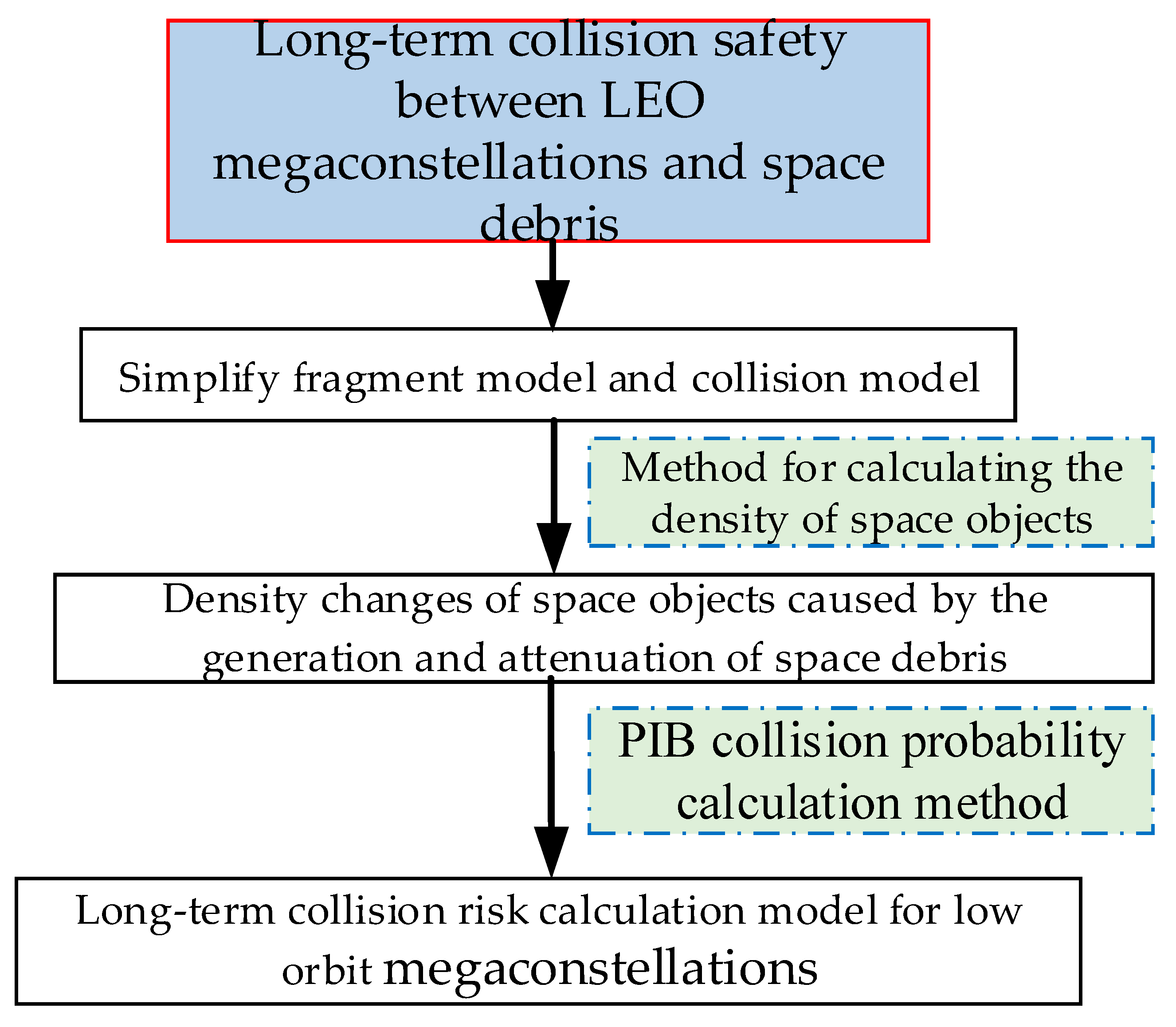
This section makes simplified assumptions about the debris and collision models, and calculates the density change of space debris in the shell where the constellation is located in accordance with the generation and death of space debris. This process is performed to avoid detailed modeling and analysis of complex scenarios for collisions in the life cycle of the constellation. A “particle-in-a-box” (PIB) collision probability calculation method is used to establish a long-term collision probability calculation model. The process of establishing the model is shown in Figure 5.

Figure 5.
Long-term collision probability calculation model.
2.2.1. Model-Simplifying Assumptions
Educated guesses and rationalized assumptions about relevant variables and their ranges are required to simplify computational models [20]. The assumptions defined in this section are as follows:
(1) All spatial objects are treated as spheres.
(2) The objects in the initial environment of LEO are divided into two groups for estimation, where the first group is the “complete objects” with a size greater than 10 cm, such as orbiting satellites and abandoned complete payloads. The radius of these objects is uniformly assumed to be 1.9 m, and the mass is 1000 kg [21]. The second group is space debris objects with a size of less than 10 cm. The radius of these debris objects is uniformly assumed to be 10 cm, and the mass is 1.2 kg [29].
(3) The calculation model for the average collision probability of an LEO megaconstellation in the shell adopts the “PIB” model [20]. The collision probability of the constellation in accordance with the density of space objects in the shell can be expressed as
where is the average collision probability of different targets, is the outer envelope radius of the satellite, is the satellite space density, is the satellite relative target velocity, V is the shell volume, is the space debris size, and is the space debris density. The formula for calculating the density of the same space object in the shell is:
(4) Assuming that the mass and cross-sectional area of the LEO megaconstellation satellites are and , the mass and cross-sectional area of the new debris generated by the collision of constellation satellites in orbit satisfy the relational expression [30]:
(5) The collision disintegration model meets the NASA collision disintegration model.
(6) The collision only produces two types of threatening space debris with a radius of 10 cm and a characteristic length sufficient to meet the collision disintegration energy, and small debris that does not pose a threat to the disintegration of the satellite.
(7) Space debris collisions with a radius of less than 10 cm do not produce new satellite-threatening debris.
(8) The debris from the collision is evenly distributed within the shell.
(9) The average relative velocity of objects colliding in LEO is 10 km/s [17,23].
(10) Targets other than the constellation satellites in the shell are considered uncontrolled, and the controlled constellation satellites will not have a collision and disintegration event.
(11) The annual failure rate of constellation satellites due to events, such as micro debris collisions or equipment failures, is 2%.
2.2.2. Space Object Density Calculation Model
Spatial density refers to the statistical value of the number of space objects contained in each cubic kilometer of volume at a certain time and a certain spatial location; the unit is 1/km3, and the calculation method is as follows [31]:
where is the size of the volume element related to the distribution of space objects, and is the number of space objects in the space volume element. needs to choose a reasonable value to reflect the distribution characteristics of space objects.
The above formula shows that that the spatial density is related to the size of the volume element and the number of objects in the volume element. However, the space objects move relative to the inertial space. At different times, the numbers of objects in the space volume element are different, the spatial density changes, and the low orbital target moves at a fast speed, so a certain instantaneous spatial density change has no practical reference importance. To better describe the density of space objects, Anselmo nd Alessandroet al. [32] introduced the concept of stay probability, averaged the instantaneous probability of space objects into the average probability over a period of time, and obtained the average density of space objects in the volume element as
where is the orbital period of the space target, and is the elapsed time of the space target entering and leaving the space volume element. On this basis, Kessler et al. made assumptions about the parameters of the target orbit and gave the calculation method for the spatial density of the object [33]:
where r is the geocentric distance; is the semi-major axis of the orbit; and are the geocentric distances of the orbit apogee and perigee, respectively. is the inclination of the target orbit, and is the declination of the target location. From the above formula, the spatial density of the space target at any height and latitude in space is obtained as
This formula requires that and . when or .
For the spatial density of the orbital height within the range of , and represent the geocentric distance of the upper and lower boundaries of the ith height interval, respectively. Zhang derived the following four formulas for solving the spatial density by averaging over the height range [25].
(1) When and , the formula for calculating the spatial density is
(2) When , , and , let , and the formula for calculating the spatial density is
When , , and , let , and the formula for calculating the spatial density is
(3) When , let and , and we obtain
If , then .
(4) In other cases, .
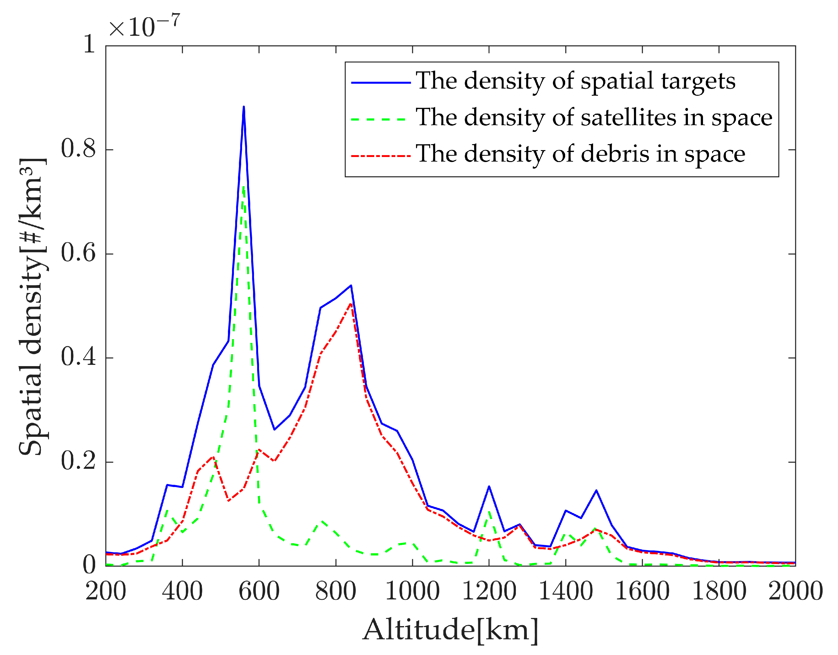
According to the density calculation formula, the density of space debris and satellites in the LEO region is calculated, and Figure 6 shows the curve of space target density with orbital altitude.
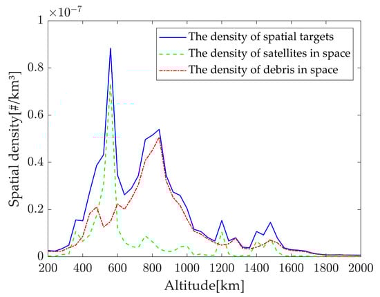
Figure 6.
The density of LEO space targets varies with orbital altitude.
2.2.3. Space Debris Attenuation Model
Taking the shell as the research object, two sources of space debris are found, where one is the inflow from the upper shell, and the other is the collision of space objects. These space debris objects are continuously attenuated under the action of atmospheric resistance and gradually flow from this shell to the next. Therefore, the density of space debris in the shell changes dynamically with time. The schematic of space debris attenuation is shown in Figure 7.
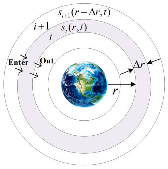
Figure 7.
Schematic of space debris attenuation.
The decay rate of the same space debris in the shell is assumed to be the same as when the debris is in the center of the shell, and the atmosphere is stationary relative to the inertial frame. The orbital decay of space debris in a period can be integrated through the perturbation equation to obtain the average decay speed of the satellite in the shell. In accordance with the calculation formula of atmospheric drag acceleration, we have
where is the atmospheric drag coefficient, A is the target area, m is the target mass, is the atmospheric density, and is the velocity vector of space debris.
The atmospheric drag acceleration is projected along the velocity direction , the geocenter radial direction , and the orbital plane normal direction . The projected components shown in Figure 8 are obtained.
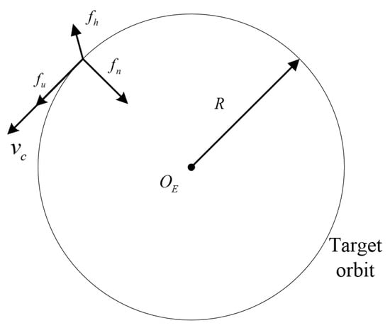
Figure 8.
Components of atmospheric drag along the direction of velocity, radial, and orbital surface normal.
Given that the velocity of the spacecraft along the radial vector direction and the normal direction of the orbital plane is zero, the components of atmospheric drag in the three directions can be obtained as
This equation is brought into the Gaussian perturbation equation of motion
where E is the anomaly angle, is the average angular velocity, and is the Earth’s gravitational constant. The perturbation motion equation is averaged over the orbital period to obtain
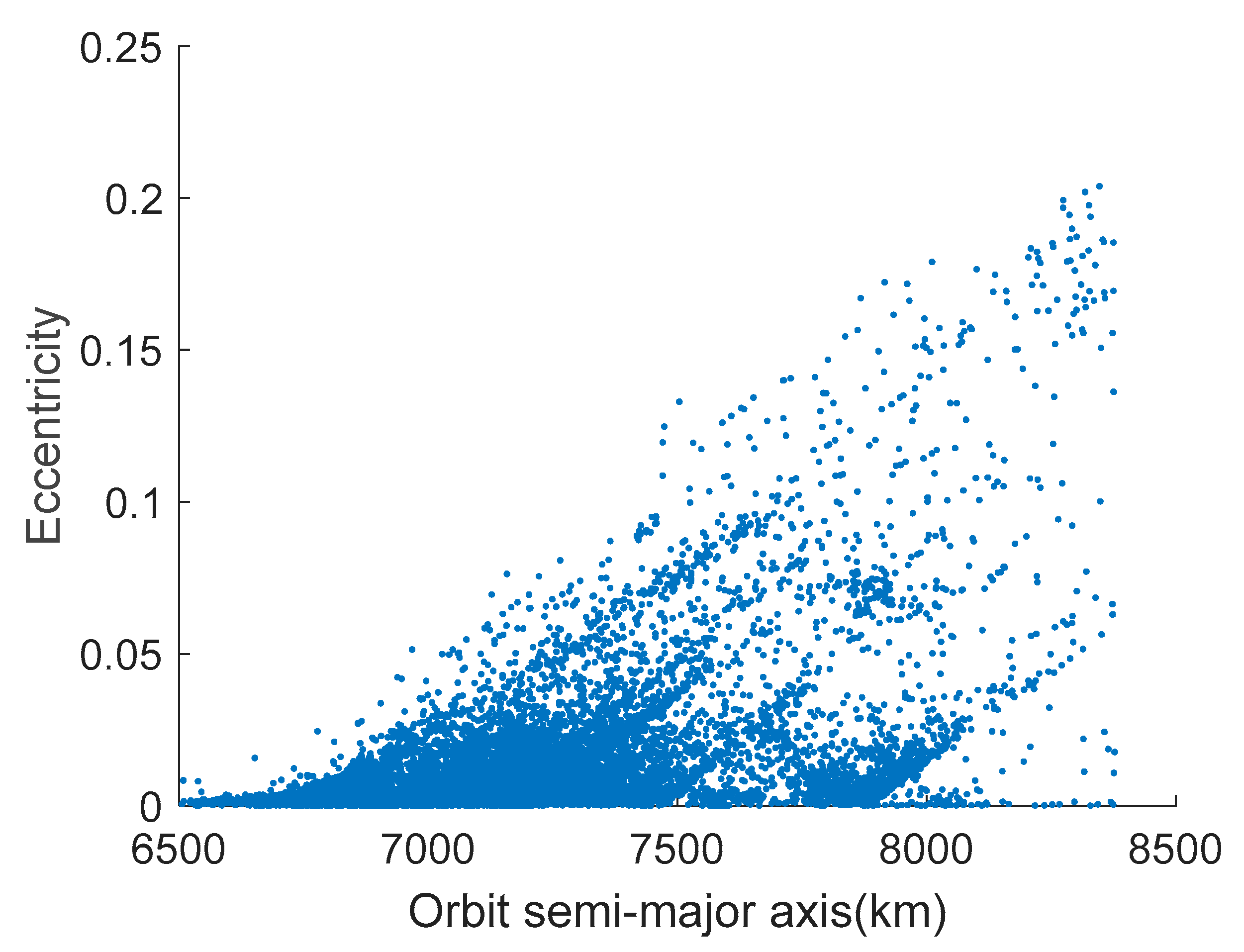
Using the Spacetrack website, 19,839 cataloged targets with an orbital height of less than 2000 km were found. The eccentricity of these cataloged targets can be counted, and the distribution of eccentricity along the semi-major axis of the orbit can be obtained, as shown in Figure 9.
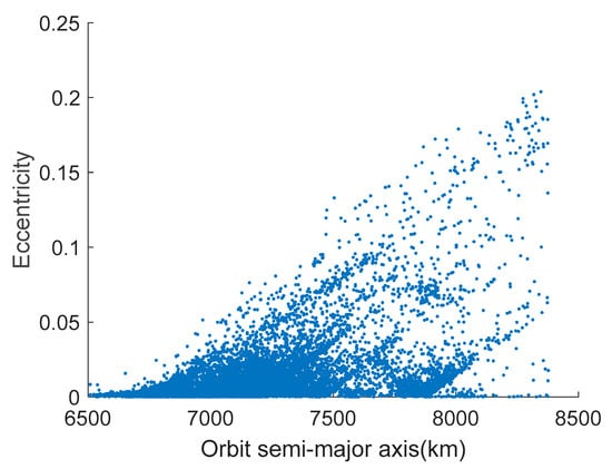
Figure 9.
Distribution of eccentricity along the semi-major axis of the track.
As shown in Figure 9, the eccentricity of most low-orbit targets is less than 0.05, and the space debris moves in approximately circular orbits in the low-orbit region. Therefore, the eccentricity of space debris can be set to zero, and the average perturbation motion of space debris in one cycle under the action of atmospheric resistance is
In accordance with Equation (42), the average decay rate of space debris in the corresponding shell is
The static atmospheric resistance in the above formula is determined by the exponential model
where , , , and .
The decay rate of space debris is relatively slow, and the heights of the far and near points do not change much during a 7-year simulation time due to the large difference in the heights of the far and near points of the large elliptical orbit, so the influence of the space density in this part of the space debris shell is ignored.
2.2.4. Space Target Collision Disintegration Model
During the long-term evolution of the constellation shell, space objects in the shell may collide, and collisions between different space objects will produce different amounts of space debris, causing different effects on the environment. Space debris is classified in accordance with the different sizes to study the specific influence of the collision of different space objects on the space environment, and the amount of space debris generated by collisions between different types of space objects and the distribution of debris in space are analyzed.
(1) Collision type investigation
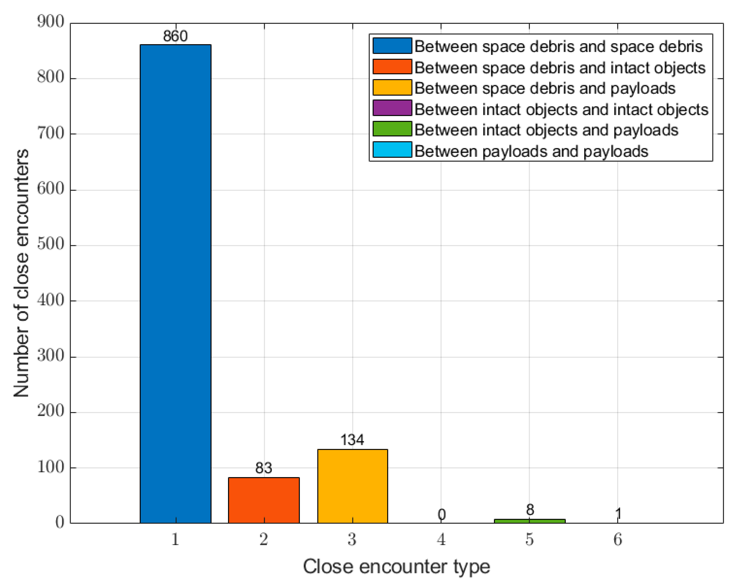
In this study, the space debris was divided into two types: cataloged debris and complete objects. In accordance with the classification, six types of collisions between space objects, which are collisions between cataloged debris and collisions between cataloged debris and space intact objects, can be obtained to catalog collisions between fragments and loads, collisions between space intact objects, collisions between space intact objects and loads, and collisions between loads and loads. In accordance with the close encounter events of space objects published on the Spacetrack website, 1086 events were selected for statistical analysis, and the distribution of different types of collision events was studied [20]. Figure 10 shows the statistics for the rendezvous target types and the numbers of rendezvous.

Figure 10.
Rendezvous target types and rendezvous statistics.
In accordance with the statistics in Figure 10, the close encounters between cataloged fragments accounted for 79.19% of the total number of encounters, the collisions between cataloged fragments and complete objects were 7.64%, and the collisions between cataloged fragments and loads were 12.34%. The collisions between loads were 0.74%, and the collisions between loads were 0.09%. Therefore, the proportions of the collision probability between various types of space objects to the total collision probability were assumed to be as follows: the collision probability between cataloged fragments accounts for 79.19% of the total, the collision probability between cataloged fragments and complete objects accounts for 19.98% of the total proportion, and the collision probability between complete objects and complete objects accounts for 0.74% of the total proportion.
(2) Spacecraft breakup model
The amounts of debris produced by the collisions of different types of space targets are different. This condition is mainly because the collision energy is different. The calculation of the collision energy can be expressed as
where represents the collision energy, is the target with smaller mass, is the target with larger mass, and is the relative motion speed. Under the condition of the same relative collision speed, the collision energy is mainly related to the mass between the two collision targets. When the collision energy is small, the collision will not cause the target to disintegrate. At present, the two targets can be completely disintegrated when the energy generated by the collision of the center of mass is greater than [34]. The collision and disintegration model of space targets adopts the American NASA collision disintegration model. In accordance with the equivalent mass of the two colliding targets, the number of space debris objects generated with different characteristic lengths can be estimated as
where is the number of space debris objects larger than the characteristic length , the characteristic length is , are the projected sizes of the space debris objects on the three orthogonal principal axes, and d is the equivalent mass of the two targets, which is expressed as
3. Simulation Results and Analysis
Orbital collisions were divided into short-term natural evolution orbital collisions and long-term orbital collisions during the constellation lifetime to evaluate the influence of constellations in different states; the TLEs were obtained from Reference [20]. This study divided the space into multiple orbital layers to facilitate the calculation. Given that the megaconstellation satellites in LEO operate at near the designed orbit, only collisions in the orbital layer where the megaconstellation is located need to be calculated.
3.1. Simulation and Analysis of Short-Term Collision Probability
3.1.1. Numerical Experimental Setup
The short-term collision probability orbit prediction model used the SGP4 model to simulate the first phase of the Starlink constellation and to facilitate the prediction of the orbit of the space cataloging target [35]. The constellation parameters of the first phase of Starlink were 1584/72/33 (1584 is the number of satellites, 72 is the number of orbit planes, and 33 is the relative spacing between satellites in adjacent planes), the orbit inclination was 53°, and the orbit height was 550 km. The shell height was 40 km, the constellation shell interval was the orbit height 530–570 km area, and the simulation time was 7 days.
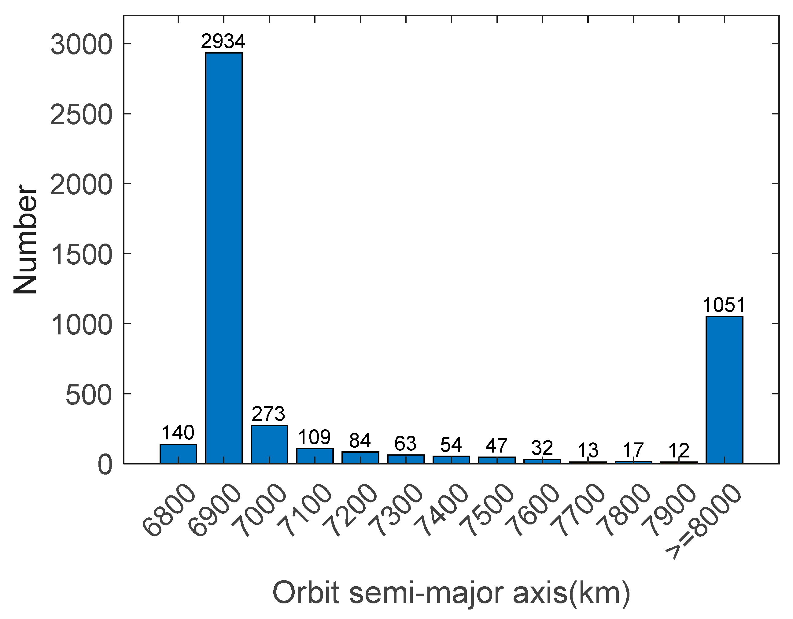
All targets cataloged on 12 March 2022 were downloaded through the Spacetrack website [20], and the apogee screening method was used to preliminarily screen the space targets. The targets with perigee greater than 570 km and the selected position less than 530 km were excluded. A total of 4829 space targets were combined with the intersection of the height intervals of the constellation shells. Taking the space debris as the statistical interval of 100 km, the orbital semi-major axis distribution of 4829 space targets was counted. Figure 11 shows the distribution of the number of space targets in accordance with the orbit semi-major axis after screening.
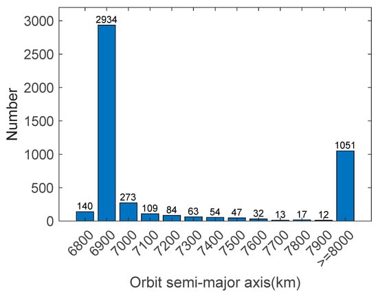
Figure 11.
Distribution map of the number of space targets remaining in the apogee–perigee screening along the semi-major axis of the orbit.
The remaining space targets were processed, and the TLE data of all satellites and space debris were converted by using STK after the invalid data were eliminated by the apogee screening method. The space targets within the shell were examined, and 653 space targets were likely to be close to space debris for a long time. The SGP4 model was used to predict the orbits of these targets and the low-orbit giant constellation satellites and long-term space targets in the shell, and the simulation step size was set to 1 s. The simulation step size was set to 5 s for the remaining 4176 space targets, and the time interval closest to the shell was solved in accordance with the orbit height, and the simulation step size of this interval was set to 1 s to perform the orbit evolution.
A total of 4176 space target orbits were screened in terms of height by using the evolved orbit data. The arcs with the height of the space target orbits in the interval of 530–570 km and their latitudes were examined. Given that the actual orbital inclination of the Starlink satellite has shifted by approximately 0.054° relative to the nominal inclination, and the random deviation between the collision target and the collision position of the satellite was considered, the latitude screening value was set to 54°.
The space discrete volume element was used to perform a preliminary approach analysis after obtaining the arcs where the space target may collide with the low-orbit giant constellation. The included angle between the adjacent orbital planes of the Starlink constellation was 5°, and the included angle between adjacent satellites in the orbital plane was about 16.3°. Therefore, the trajectory of the space target in the space volume element needed to be increased as much as possible to minimize the number of satellite targets in the space. The values of space volume elements were set to 40 km, 4.8°, and 9°, respectively. In accordance with the space targets that appeared in the same space volume element at the same time, the relative distances were calculated pairwise by using the orbit data, and the distance to the closest trajectory point and the “” distance were judged to remove possible collision targets.
3.1.2. Results and Analysis
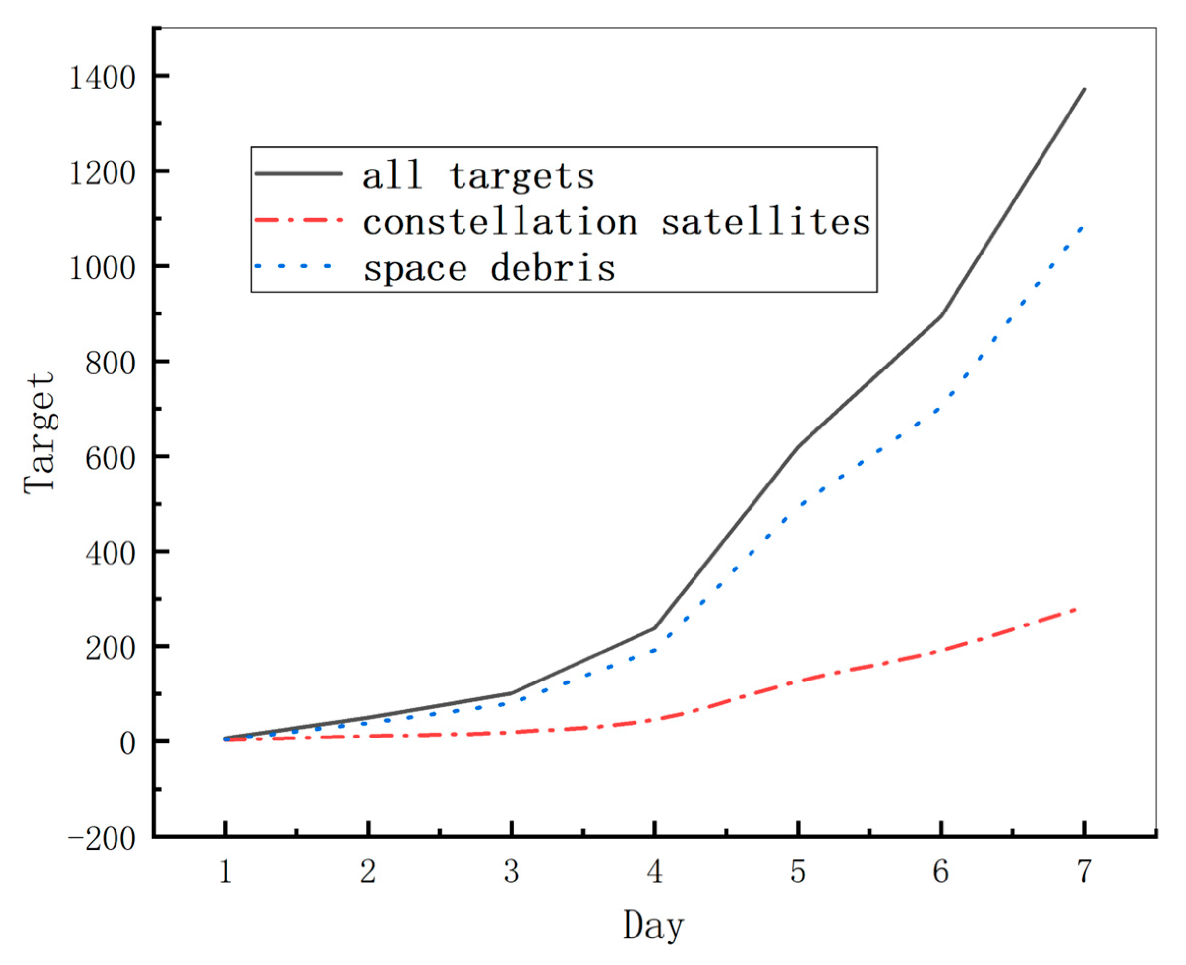
In accordance with the filtered data, a large portion of the space targets were close to each other for a long time. For this part of the target data, the orbital period of the space target was used to calculate the closest distance of the trajectory point in each period, and the closest distance to the trajectory point and its vicinity were considered. This trajectory point was the most likely to collide, and other trajectory points would not collide, thereby eliminating other trajectory points in each orbital cycle of the target. The approaching situation of the space target within 7 days was obtained after eliminating the long-term approaching target data. Figure 12 shows the statistics for different types of proximity situations.
Figure 12.
The statistics for different types of proximity situations.
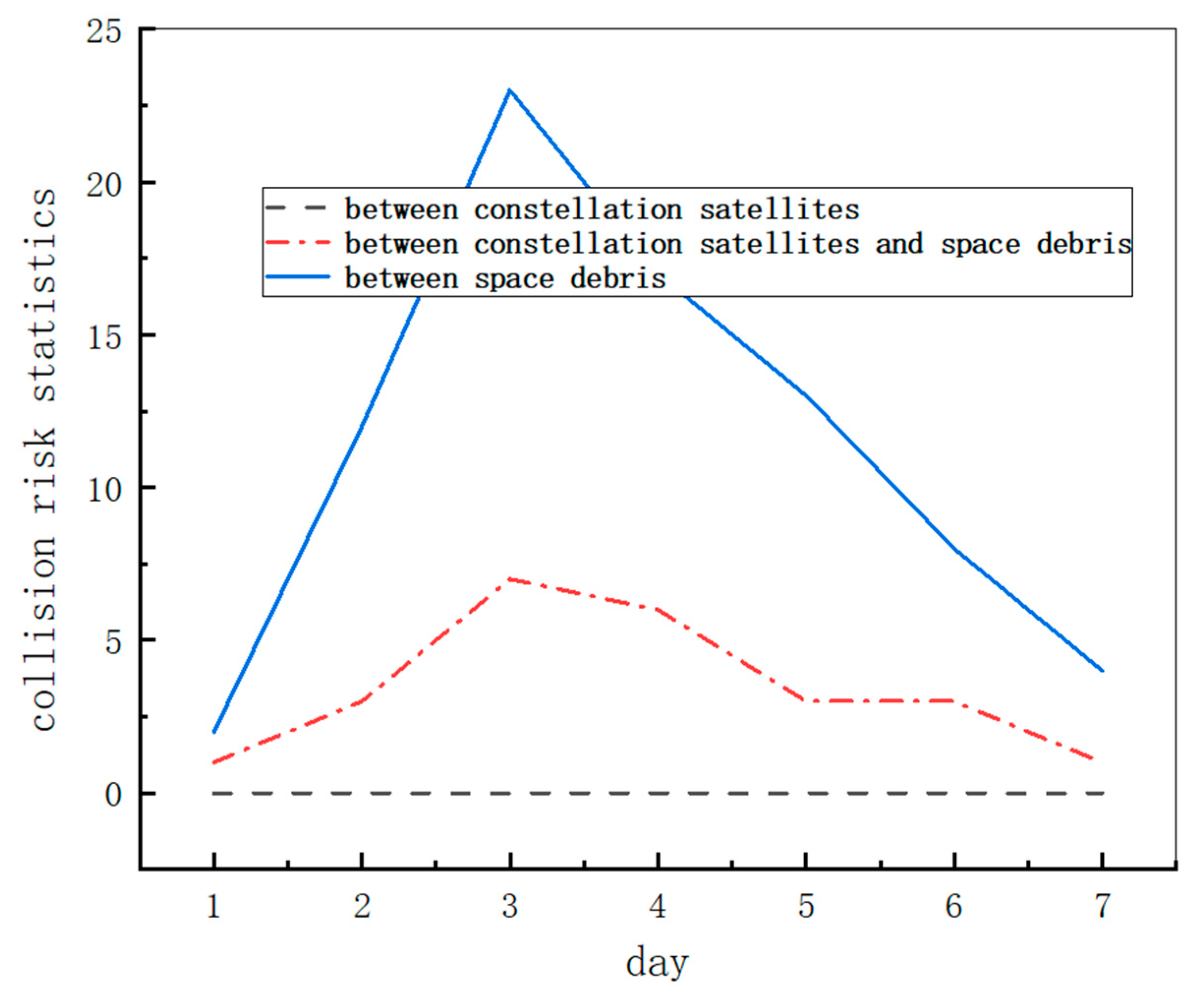
As shown in Table 2, many close points will be missed when the ellipsoid error is small due to the small relative screening distance. With the gradual increase in error, the relative screening distance and the number of targets that meet the proximity conditions increased. The time of the closest track point retained was filtered in accordance with the relative distance, and two points were selected before and after the track point. Lagrangian interpolation was used to calculate the closest moment and the motion state of the two targets at that moment and bring them into the Laplacian-based method. The collision probability calculation method of the Si transform was used to obtain the collision risk situation of the space target. Figure 13 shows the collision probability of space rendezvous targets greater than 10−5 times.
Table 2.
Close proximity of space targets in the shell.
Figure 13.
Collision frequency of space rendezvous targets greater than 10−5 times.
As shown in Table 3, the number of collisions between constellation satellites and space debris greater than reached seven times within the 7-day simulation period. The collision risk increased by about 30% to 40% after the constellation was deployed compared with before the deployment of the constellation by comparing the number of constellation satellites with a collision probability greater than and the number of collisions between space debris with a probability greater than .
Table 3.
Collision frequency of space rendezvous targets greater than 10−5 times.
3.2. Simulation and Analysis of the Long-Term Collision Probability
3.2.1. Numerical Experimental Setup
The long-term collision probability simulation calculation of the first phase of the Starlink constellation was performed. The known constellation parameters were 1584/72/33, the orbit height was 550 km, the orbit inclination was 53°, the satellite mass was 260 kg, and the satellite size was . The simulation time was 7 years and the constellation shell height H = 40 km.
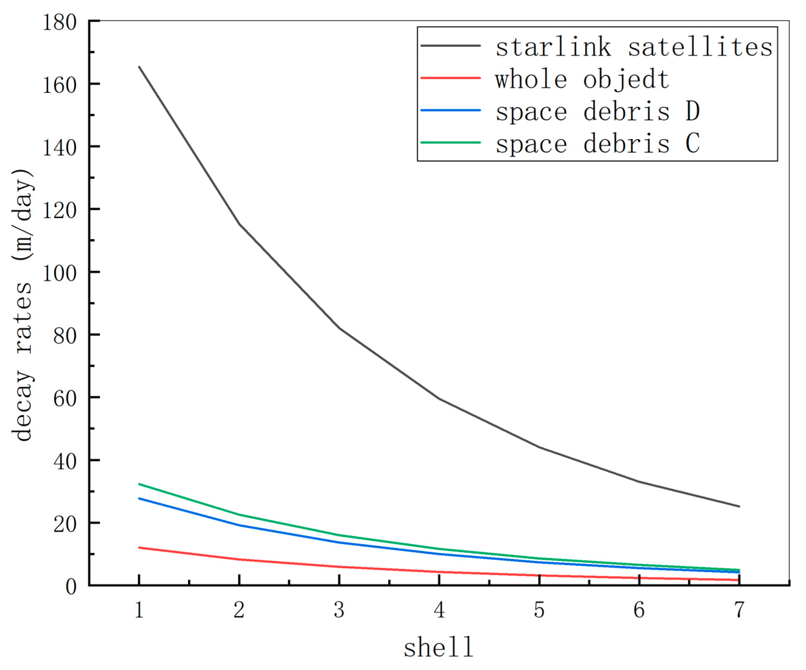
Considering that the atmospheric resistance can be approximately ignored when the orbit height is greater than 800 km, the shell was divided into seven intervals in accordance with the orbit height of the Starlink constellation, and the interval height range was 530–810 km. From Assumption 6 and Formula (48), the mass of space debris that reaches the collision disintegration energy was 0.208 kg. From Assumption 4, the cross-sectional area of the space debris of type could be obtained as 0.0065 m2, and the radius of the space debris of type could be obtained as 0.045 m. In accordance with the definition of the characteristic size, the attenuation speed of the space target in each shell could be obtained by using the static atmospheric drag density model after the surface-to-mass ratio and orbit height of the space target were known. Figure 14 shows the different decay rates of the targets in each shell.
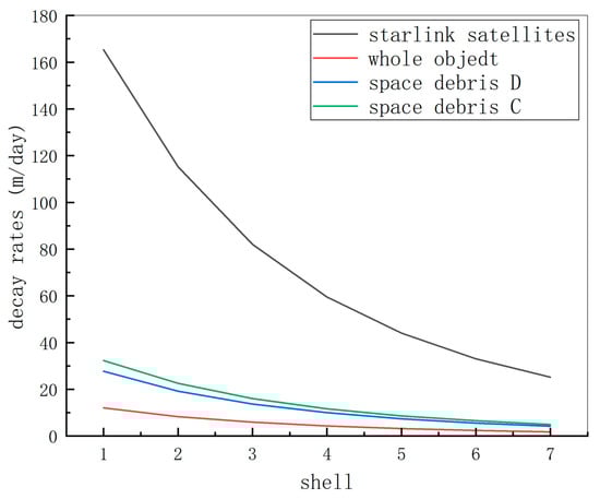
Figure 14.
The different decay rates of the targets in each shell.
Table 4 presents the decay rates of various targets within each shell. Notably, the decay rates of the Starlink satellites surpass that of other targets by a significant margin.
Table 4.
Relationship between the decay rates and the shell of the different types of space targets.
The space debris environments in the shells could be obtained from the existing cataloging data. The cataloging target data could be downloaded from the Spacetrack website, and the download date was 12 March 2022. The downloaded cataloging targets were screened in terms of the shells, and each item at the initial moment could be obtained. The numbers of space debris objects were cataloged for each shell. Figure 15 shows the distribution of the numbers of space debris objects in each shell.
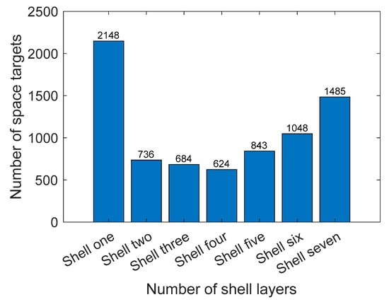
Figure 15.
Distribution map of the number of space debris objects in each shell.
In accordance with the statistics in [10], the number of rocket bodies in the low-orbit area was 916 and the number of loads was 6420 as of 4 April 2022. Assuming that the distribution of rocket bodies was proportional to the number of loads, Starlink could be obtained through the Spacetrack website. The number of satellites in the first shell was 1495, and the number of other payloads and space debris objects in the first shell was 653. Therefore, the number distribution of the rocket bodies in each shell and the statistics on the number of satellites in each shell could be obtained, and the number of complete objects in each shell could be calculated. Table 5 shows the distribution of complete debris types I and D in the shells.
Table 5.
Quantity distribution of the different types of space debris in the shells.
3.2.2. Results and Analysis
The number of space debris objects in a shell is the number of debris objects in this shell plus the number of debris objects entering the higher shell and the number of debris objects falling out of this shell. In accordance with Table 4 and Table 5, the amount of space debris in the constellation life cycle of the first shell due to orbital decay changed as follows:
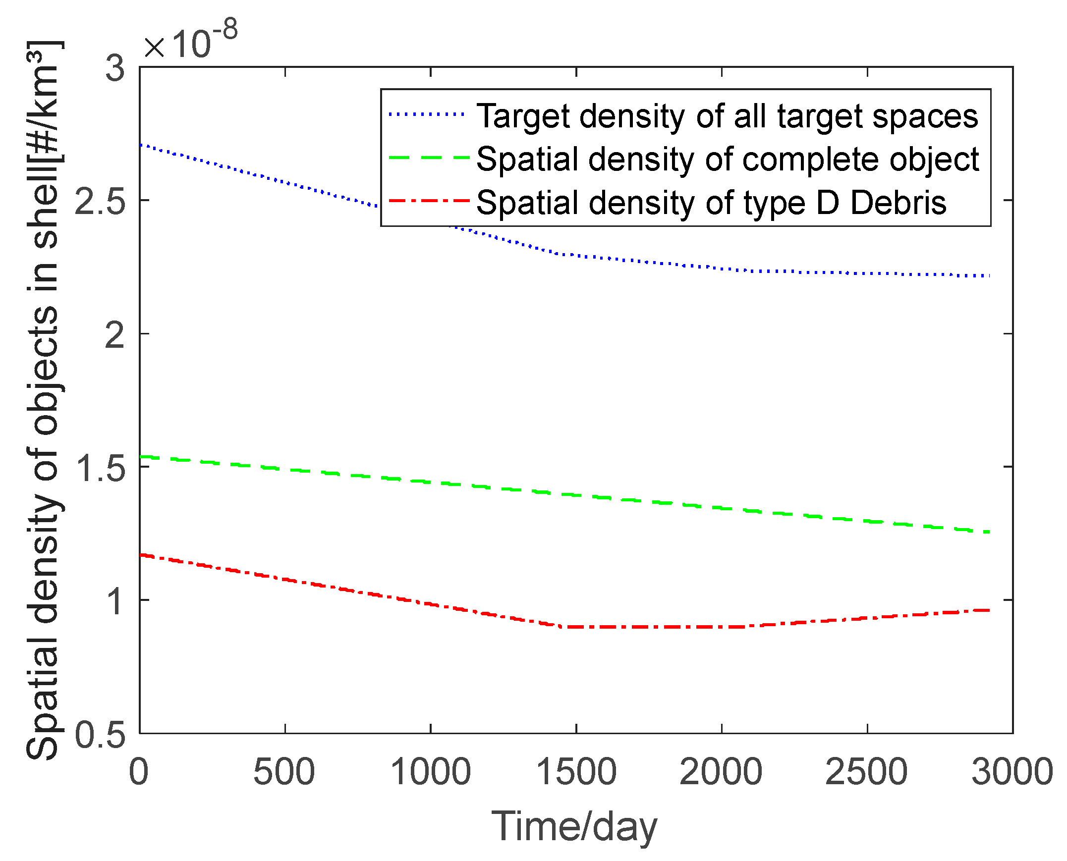
where is the number of debris objects, subscripts represent the type of the i-th shell fragment, is the decay speed, and is the number of days. In accordance with the definition of density , the evolution relationship of the space environment density with time during the life cycle of the Starlink constellation could be obtained. Figure 16 shows the spatial density evolution of background debris in the shell.
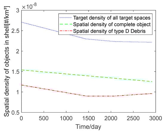
Figure 16.
Spatial density evolution of background debris in the shell.
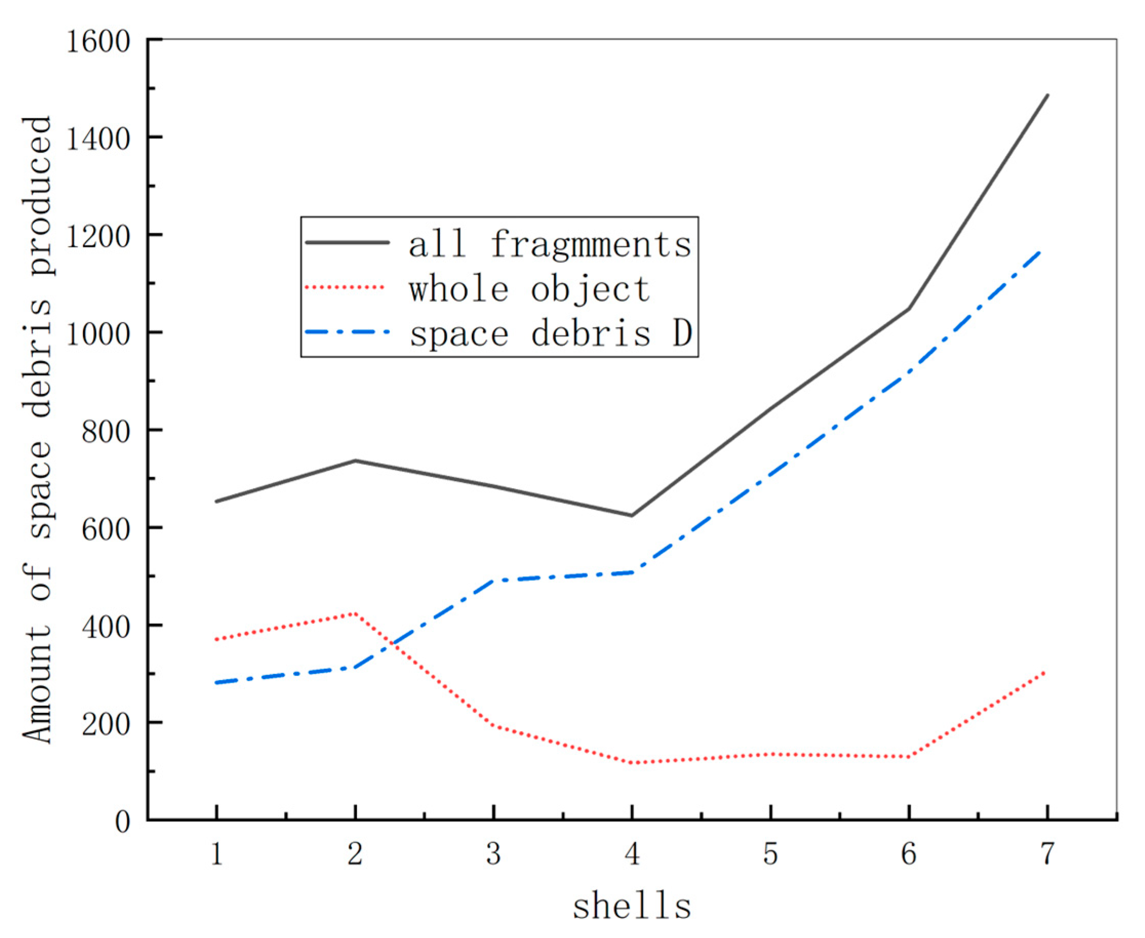
In accordance with the assumption, the space debris only collided with the failed Starlink satellites. Up to 32 satellites failed each year at the failure ratio of 2%. Given that the satellites decayed at a rate of 165.4 m per day in the shell, the satellites were assumed to be evenly distributed in the shell. In 4 months, half of the satellites fell out of the shell due to attenuation. Although 32 satellite failures occurred in the first and second year, the spatial density of the failed satellites reached a maximum of , which was still lower than the background. If no collision event occurred in space during the lifetime of the constellation, the spatial density was reduced by 4–16.7% compared with that before the deployment of the constellation. Starlink satellites and intact objects generated new space debris due to collision. Therefore, the collision disintegration events were divided into six types, and the amount of space debris generated by different collision events was calculated. Figure 17 shows the amount of space debris generated by different collision types.
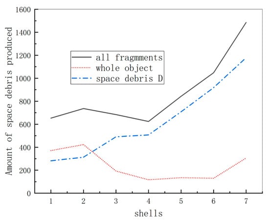
Figure 17.
The amount of space debris generated by different collision types.
As shown in Table 6, a large amount of debris was generated in one collision, the least one collision generated was approximately 200 space debris objects, and the density increased. In accordance with the average value of the debris generated, the generated space debris objects reached 658, the density increased, and the space debris increased. The density was double that when the constellation was not deployed. In accordance with Table 4, the generated space debris has a small surface mass ratio, a low orbital decay rate, and the debris has a long residence time in the orbit, resulting in long-term collision risks for the constellation in orbit. The risks are multiplied, and in-orbit collisions with satellites should be avoided as much as possible.
Table 6.
Amount of space debris produced by different collision types.
Taking the Starlink constellation as an example, the short-term collision probability and long-term collision probability of the constellation were calculated, and the results are as follows:
(1) The probability of collision between Starlink Phase I constellation satellites and space debris is greater than seven times a day. Compared with that before the deployment of the constellation, the collision frequency in the shell increases by about 30–40%, indicating that the collision risk faced by a satellite is higher than that before the deployment of the constellation. The satellite needs to have better orbital maneuvering and collision warning abilities.
(2) During the 7-year evolution period of the Starlink constellation, the average collision probability after the deployment of the Starlink constellation does not increase compared with that for the nondeployed constellation, indicating that a lower constellation orbit height can improve the orbital safety and space environment stability of a low-orbit giant constellation.
(3) The occurrence of a collision greatly increases the density of space debris, and the space debris generated by the collision is small and stays in orbit for a long time, resulting in a greater threat of secondary collisions to constellation satellites.
4. Conclusions
This paper investigates the collision safety of LEO megaconstellations under the current space debris environment. A collision evolution calculation method for large-scale space debris and large-scale satellites is proposed. By filtering and partitioning data, the computing efficiency is improved while satisfying high accuracy.
The lower orbital altitude of the Starlink constellation improves the safety of the constellation and the stability of the space environment, but the collision risk faced by the constellation is still high. A satellite needs to have good orbital maneuverability and collision warning capabilities. The risk of a second collision in a constellation increases exponentially.
This study has proposed a calculation method for the collision safety assessment parameters of an LEO megaconstellation. The short-term collision probability and long-term average collision probability of the constellation are used to evaluate the safety of the constellation to improve the reliability and effectiveness of the constellation safety assessment. Through a simulation of the Starlink Phase I constellation, the results show that after the deployment of the Starlink constellation, the probability of a short-term collision in the constellation shell increases by 30–40%, the probability of at least one collision in the constellation lifetime is 70.2%, and the probability of a secondary collision increases by 25.3% after a collision. These models not only offer insights into orbital safety but also present valuable references and practical applications. The innovative findings of this study introduce novel methodologies and concepts to effectively mitigate the risks associated with constellation collisions.
The main topics for possible future improvements are as follows. Space debris has become a growing problem in the space sector, and the deployment of large constellations consisting of hundreds or thousands of satellites is an environmental concern. The occurrence of a collision causes more serious consequences. The method for how to avoid the collision of constellation satellites and improve the safety of constellation in-orbit operation should be further investigated. Building upon existing research, there is a need to refine perturbation and collision models while considering the distribution and evolution of fragments post-collision. This involves integrating evaluation models and exploring objective, simple, easily verifiable, and replicable methods to assess the LEO spatial environment. Furthermore, expanding the scope of research to encompass other constellations under construction or already operational is essential, including the consideration of various collision scenarios such as satellite-to-satellite collisions and collisions involving space devices. This expanded approach will facilitate a more comprehensive evaluation of collision risks across different scenarios.
Author Contributions
Conceptualization, M.H. and C.Y.; methodology, C.Y.; simulation, C.Y. and W.X.; writing—original draft preparation, C.Y. and Y.R.; writing—review and editing, Y.R.; visualization, Y.R.; supervision, M.H. All authors have read and agreed to the published version of the manuscript.
Funding
This research received no external funding.
Data Availability Statement
The data are available from the corresponding author on reasonable request. Data access is restricted to research and educational applications.
Conflicts of Interest
The authors declare no conflicts of interest.
References
- Bernat, P. Orbital satellite constellations and the growing threat of Kessler syndrome in the lower Earth orbit. Inżynieria Bezpieczeństwa Obiektów Antropog. 2020, 4, 1–14. [Google Scholar] [CrossRef]
- ESA Space Debris Office, Space Debris. 2023. Available online: https://www.esa.int/Space_Safety/Space_Debris/Space_debris_by_the_numbers (accessed on 21 March 2024).
- Lifson, M.; Arnas, D.; Avendaño, M.; Linares, R. A Method for Generating Closely Packed Orbital Shells and the Implication on Orbital Capacity. In Proceedings of the AIAA SCITECH Forum, National Harbor, MD, USA, 23–27 January 2023; p. 2170. [Google Scholar]
- Chen, Q.; Yang, L.; Zhao, Y.; Wang, Y.; Zhou, H.; Chen, X. Shortest Path in LEO Satellite Constellation Networks: An Explicit Analytic Approach. IEEE J. Sel. Areas Commun. 2024, 1–13. [Google Scholar] [CrossRef]
- Ruan, Y.; Hu, M.; Yun, C. Advances and prospects of the configuration design and control research of the LEO mega-constellations. Sci. China Technol. Sci. 2022, 42, 1. [Google Scholar]
- Jonathan. Starlink Statistics. 2023. Available online: https://planet4589.org/space/stats/star/starstats.html (accessed on 8 June 2023).
- Chen, Q.; Giambene, G.; Yang, L.; Fan, C.; Chen, X. Analysis of Inter-Satellite Link Paths for LEO Mega-Constellation Networks. IEEE Trans. Veh. Technol. 2021, 70, 2743–2755. [Google Scholar] [CrossRef]
- Hindin, J.D. Application for Fixed Satellite Service by Kuiper Systems LLC [SAT−LOA−20190704−00057]. 2022. Available online: https://fcc.report/IBFS/SAT−LOA−20190704−00057 (accessed on 21 March 2024).
- Sun, H.; Zhang, Z. Study on space environment safety based on satellite collision. IOP Conf. Ser. Earth Environ. Sci. 2020, 552, 012014. [Google Scholar] [CrossRef]
- European Space Agency. “ESA’s Space Environment Report” ESA’s Space Debris Office. 2022. Available online: https://www.esa.int/Space_Safety/Space_Debris/ESA_s_Space_Environment_Report_2022 (accessed on 21 March 2024).
- ESA Space Debris Office, Space Environment Statistics. 2022. Available online: https://sdup.esoc.esa.int/discosweb/statistics/ (accessed on 21 March 2024).
- Radtke, J.; Kebschull, C.; Stoll, E. Interactions of the space debris environment with mega constellations—Using the example of the OneWeb constellation. Acta Astronaut. 2017, 131, 55–68. [Google Scholar] [CrossRef]
- Miraux, L. Environmental limits to the space sector’s growth. Sci. Total Environ. 2022, 806, 150862. [Google Scholar] [CrossRef]
- Tao, H.; Zhu, Q.; Che, X.; Li, X.; Man, W.; Zhang, Z.; Zhang, G. Impact of Mega Constellations on Geospace Safety. Aerospace 2022, 9, 402. [Google Scholar] [CrossRef]
- Olivieri, L.; Francesconi, A. Large constellations assessment and optimization in LEO space debris environment. Adv. Space Res. 2020, 65, 351–363. [Google Scholar] [CrossRef]
- Isoletta, G.; Opromolla, R.; Fasano, G. Uncertainty-aware Cube algorithm for medium-term collision risk assessment. Adv. Space Res. 2023, 71, 539–555. [Google Scholar] [CrossRef]
- Adilov, N.; Braun, V.; Alexander, P.; Cunningham, B. An estimate of expected economic losses from satellite collisions with orbital debris. J. Space Saf. Eng. 2023, 10, 66–69. [Google Scholar] [CrossRef]
- Campiti, G.; Brunetti, G.; Braun, V.; Di Sciascio, E.; Ciminelli, C. Orbital kinematics of conjuncting objects in Low-Earth Orbit and opportunities for autonomous observations. Acta Astronaut. 2023, 208, 355–366. [Google Scholar] [CrossRef]
- Carmen, P.; Luciano, A. Using the space debris flux to assess the criticality of the environment in low Earth orbit. Acta Astronaut. 2022, 198, 756–760. [Google Scholar]
- Rossi, A.; Farinella, P. Collision rates and impact velocities for bodies in low Earth orbit. ESA J. 1992, 16, 339–348. [Google Scholar]
- Chuan, C.H.; Wulin, Y.A.; Zizheng, G.O.; Pinliang, Z.H.; Ming, L.I. Analysis of the impact of large constellations on the space debris environment and countermeasures. Aerosp. China 2020, 21, 16–22. [Google Scholar]
- Lewis, H.G. Understanding long-term orbital debris population dynamics. J. Space Saf. Eng. 2020, 7, 164–170. [Google Scholar] [CrossRef]
- Le May, S.; Gehly, S.; Carter, B.; Flegel, S. Space debris collision probability analysis for proposed global broadband constellations. Acta Astronaut. 2018, 151, 445–455. [Google Scholar] [CrossRef]
- Lewis, H.G. Evaluation of debris mitigation options for a large constellation. J. Space Saf. Eng. 2020, 7, 192–197. [Google Scholar] [CrossRef]
- Polli, E.M.; Gonzalo, J.L.; Colombo, C. Analytical model for collision probability assessments with large satellite constellations. Adv. Space Res. 2022, 72, 2515–2534. [Google Scholar] [CrossRef]
- Pardini, C.; Anselmo, L. Assessing the risk of orbital debris impact. Space Debris 1999, 1, 59–80. [Google Scholar] [CrossRef]
- Ana, S.R.; Claudio, B.; Rafael, V. Short-Term Space Occupancy and Conjunction Filter. arXiv 2023, arXiv:2309.02379. [Google Scholar]
- Zhang, W.; Wang, X.; Cui, W.; Zhao, Z.; Chen, S. Self-induced collision risk of the Starlink constellation based on long-term orbital evolution analysis. Astrodynamics 2023, 7, 445–453. [Google Scholar] [CrossRef]
- Chan, F.K. Spacecraft Collision Probability; Aerospace Press: El Segundo, CA, USA, 2008; pp. 1–12. [Google Scholar]
- Anselmo, L.; Pardini, C. Dimensional and scale analysis applied to the preliminary assessment of the environment criticality of large constellations in LEO. Acta Astronaut. 2019, 158, 121–128. [Google Scholar] [CrossRef]
- Pardini, C.; Anselmo, L. Review of past on-orbit collisions among cataloged objects and examination of the catastrophic fragmentation concept. Acta Astronaut. 2014, 100, 30–39. [Google Scholar] [CrossRef]
- Anselmo, L.; Cordelli, A.; Pardini, C.; Rossi, A. Space Debris Mitigation Extension of the SDM Tool; European Space Agency: Pisa, Italy, 2000. [Google Scholar]
- Kessler, D.J. Derivation of the collision probability between orbiting objects: The lifetimes of Jupiter’s outer moons. Icarus 1981, 48, 39–48. [Google Scholar] [CrossRef]
- McKnight, D.S. Collision and Breakup Models: Pedigree, Regimes, and Validation/Verification. In Proceedings of the National Research Council Committee on Space Debris Workshop, Irving, CA, USA, 18–20 November 1993. [Google Scholar]
- Rossi, A.; Petit, A.; McKnight, D. Short-term space safety analysis of LEO constellations and clusters. Acta Astronaut. 2020, 175, 476–483. [Google Scholar] [CrossRef]


Disclaimer/Publisher’s Note: The statements, opinions and data contained in all publications are solely those of the individual author(s) and contributor(s) and not of MDPI and/or the editor(s). MDPI and/or the editor(s) disclaim responsibility for any injury to people or property resulting from any ideas, methods, instructions or products referred to in the content. |
© 2024 by the authors. Licensee MDPI, Basel, Switzerland. This article is an open access article distributed under the terms and conditions of the Creative Commons Attribution (CC BY) license (https://creativecommons.org/licenses/by/4.0/).