Abstract
The impact of a lightning electromagnetic pulse (LEMP) on a power line or power station produces an effect similar to that of switching between a significant power source and a power line circuit. This switch closure causes a sudden change in routing conditions, creating a transient state. This situation has been studied in terms of electrostatic and electromagnetic induction, as well as overvoltage changes. Appropriate mathematical models were used to analyze these changes. While vertical electric field analysis has been carried out in a few studies, magnetic field and horizontal electric field vectors have not been studied. In this study, the Rusck formulation and the Heidler current formulation are combined at the current level, developed and analyzed. This is because the Rusck expression can sometimes give incorrect results at the current level. Also, in the analysis, electromagnetic field formulations based on accelerating charges are used instead of the dipole approximation to eliminate the need for interpolation in the graphical results. In contrast to other studies in the literature, this study proposes the use of moving and accelerating load techniques to better understand the effects of LEMPs on power transmission lines. Also, in this study, the double exponential problem of the current form in Rusck’s formulation is addressed in order to obtain a close approximation of the physical form of the LEMP. Additionally, the field–line (coupling) relationship is studied according to a unique closed formulation, leading to important determinations about the overvoltages generated on a line depending on the propagation speed of the LEMP sprout and the electrical changes in the area where the LEMP first occurs.
1. Introduction
Lightning activity has become a major cause of intermittent disturbances in power systems, significantly affecting the quality of power distribution. This is due to the fact that high-, medium- and low-voltage lines are more elevated than surrounding buildings, making them more susceptible to direct or indirect lightning electromagnetic pulses (LEMPs). K.W. Wagner carried out a primary hypothetical investigation of lightning-induced surges in power transmission lines with the following objectives: This research investigated the reasons for lightning strikes on transmission lines [1]. In 1929, Bewley utilized Wagner’s hypothesis to reveal that the field induced by lightning cannot vanish immediately [2]. An article written by Aigner in 1935 was the first in the current literature to consider the inducing effect of vertical lightning paths on the ground due to a lightning strike [3]. In an editorial distributed in 1948, Szpor, unlike Wagner and McCann, calculated the induced voltages resulting from vertical lightning strikes using more complex assumptions. Szpor claimed it was essential to consider the magnetic impact in addition to the electrostatic effects. The study emphasized that this consideration is significant for the regions near a lightning strike point [4]. In 1958, Rusck calculated induced voltages for energy transmission lines (ETLs) with short and long ranges and developed a closed-form expression with a global standard [5,6]. Rusck’s approach failed to consider a precise analytical formulation for vertical electric fields (VEFs), which was developed by Andreotti et al. [7]. Compared to Rusck’s results, Andreotti et al.’s study pointed out differences in the surge voltages caused by an LEMP. Although Rusck also addressed this issue, its practical effects on different LEMP flows and overhead lines have not been studied in detail. Therefore, there is a need for an in-depth investigation of Rusck’s impact on the calculation of electric areas, induced voltages and the indirect lightning performance of overhead lines. A similar study was carried out for medium-voltage lines. In this study, the LEMP status was investigated using the 3D finite-difference time-domain (FDTD) method. It is advantageous for analyzing LEMP because it can handle non-uniform conductors over lossy ground [8]. Another study determined the current and electric field values of lightning’s return stroke [9]. Induced voltages and fields were investigated based on the lightning strike angle with a constant current value by B. V. Amin Foroughi Nematollahi [10]. Farhan Mahmood carried out insulation work to protect against lightning-induced overvoltages in medium-voltage overhead lines [11]. In a similar literature study, a numerical analysis of both the lightning current pulse and the electromagnetic field propagating in the far field was performed using a revised modified transmission line model with exponential decay (MTLE) for high-rise buildings with conductive ground [12]. In another work, theoretical models, numerical simulations and experimental tests for determining the pulses propagating between the windings of transformers subjected to lightning strikes were discussed [13]. In another study, the impact of a grounded wind tower, ground conductivity, permittivity, the depth of the cable and its position from the return stroke on the lightning-induced electromagnetic fields on a cable sheath was investigated [14]. In another work in the literature, a new numerical method was proposed to reconstruct the waveform of a distant electric field due to a lightning strike on a tall structure [15]. In another literature study, an approximate formula was proposed for evaluating the peak values of lightning-induced voltages in the presence of highly resistive soils [16]. Finally, another recent study in the literature discussed the widespread use of the FDTD method, one of the full-wave numerical approaches, to simulate electromagnetic transients in earthing structures, such as earthing grids for substations [17].
In this study, overvoltages, electrostatic induction and electromagnetic induction changes, which occur due to LEMPs, indirectly affecting power plants, were investigated using Rusck’s equations. The surge protection systems on power transmission lines exposed to indirect effects did not function as intended. This is because surge arresters are designed to protect against the main shock pulse of an LEMP. In our study, the issue lay in the propagation of the main shock pulse to the ground. We investigated the situations arising from the induction of this propagated shock current on nearby lines. We view this situation as an interference problem from an electromagnetic compatibility perspective. The research is believed to be beneficial for future studies in the fields of power systems and electromagnetic compatibility, particularly in terms of grounding and electromagnetic shielding.
In this study, we analyze the indirect effects of LEMPs occurring close to power transmission lines. The motivation for this analysis stems from the inadequacy of surge arrester systems in fully mitigating indirect effects. While surge arresters offer protection against the main shock pulse of the LEMP when it directly impacts the line, they fall short in addressing indirect effects. Our study focuses on investigating the parasitic currents, electric field and magnetic field values contributing to this issue.
The Rusck model served as the coupling model for this study’s energy transmission line. Rusck’s equations are commonly used to analyze the indirect effects of lightning electromagnetic pulses on power distribution and transmission lines. This is because the LEMP channel is typically assumed to be vertical in such analyses. Compared to other modeling approaches, Rusck’s expressions can be used in engineering studies without any disadvantages. Additionally, the analytical expression provided by Rusck enables easy calculation of the electric field from the return pulse of the LEMP. The Heidler Wave model was exemplified as the source of LEMPs. Substantial results were obtained by examining the relationship between the areas and the line according to the Rusck formulation. This study was conducted mathematically. Mathematical modeling was performed using MATLAB version R2023A.
The main focus of this study was the lack of sufficient research in the field of electromagnetic compatibility for the LEMP phenomenon. This situation causes significant damage to power transmission lines, especially in countries where LEMP strikes are intensive and in high-altitude regions. Particularly in the regions we examined, the transmission lines supply power to industrial areas, and LEMP attacks in these areas often lead to prolonged power outages. This is one of the driving factors behind this research. Considering the intensity of studies in the field of power systems, we believe that protective methods in terms of electromagnetic compatibility (such as electromagnetic shielding and satellite grounding applications) could be effective at preventing these indirect effect faults on the lines.
2. Theoretical Background and Mathematical Models
2.1. Direct LEMP Drop
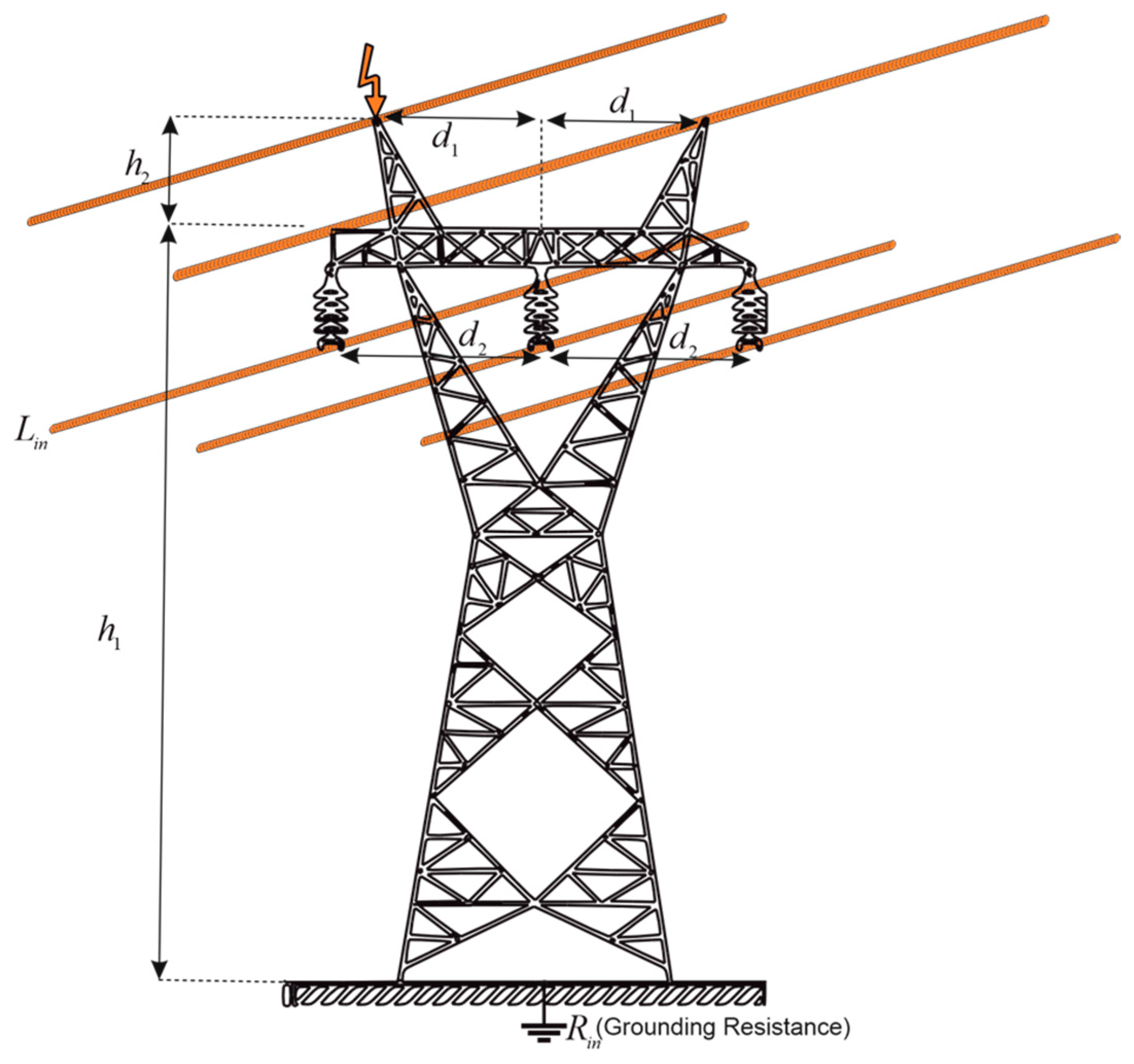
Figure 1 represents the direct discharge of LEMPs onto any part of an electrical network. In most cases, due to high overvoltages in ETLs compared to the insulation level, deterioration occurs in the insulations even though the return current is small. Therefore, during direct strikes, overvoltages on lines can cause damage or the breakage of insulation materials [18].
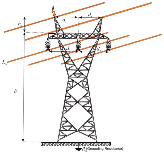
Figure 1.
Direct drop of LEMPs on ETLs (h: the height of the transmission line, d1,2: the distance between insulators, h1,2: console height, Lin: conductor length).
2.2. Indirect LEMP Drop
An indirect LEMP discharge does not directly strike any portion of a power system. However, it generates an induced overvoltage that propagates throughout the network. This type of LEMP discharge can cause interruptions in low-insulation lines (low-protection transmission lines). Although indirect pulses produce smaller inductive voltages compared to direct strikes, they often affect the performance of overhead lines. For example, indirect pulses on medium-voltage lines are the primary source of recorded faults. In studies on indirect LEMPs, two variants of the dipole technique are commonly employed: a continuity equation technique and a technique based on moving and accelerating charges. These techniques are used in the literature to evaluate electromagnetic fields after the spatial and temporal distribution of the current is given. This study employed the technique based on moving and accelerating charges to express the electromagnetic fields analytically.
2.3. Lightning Electromagnetic Pulse Current Models
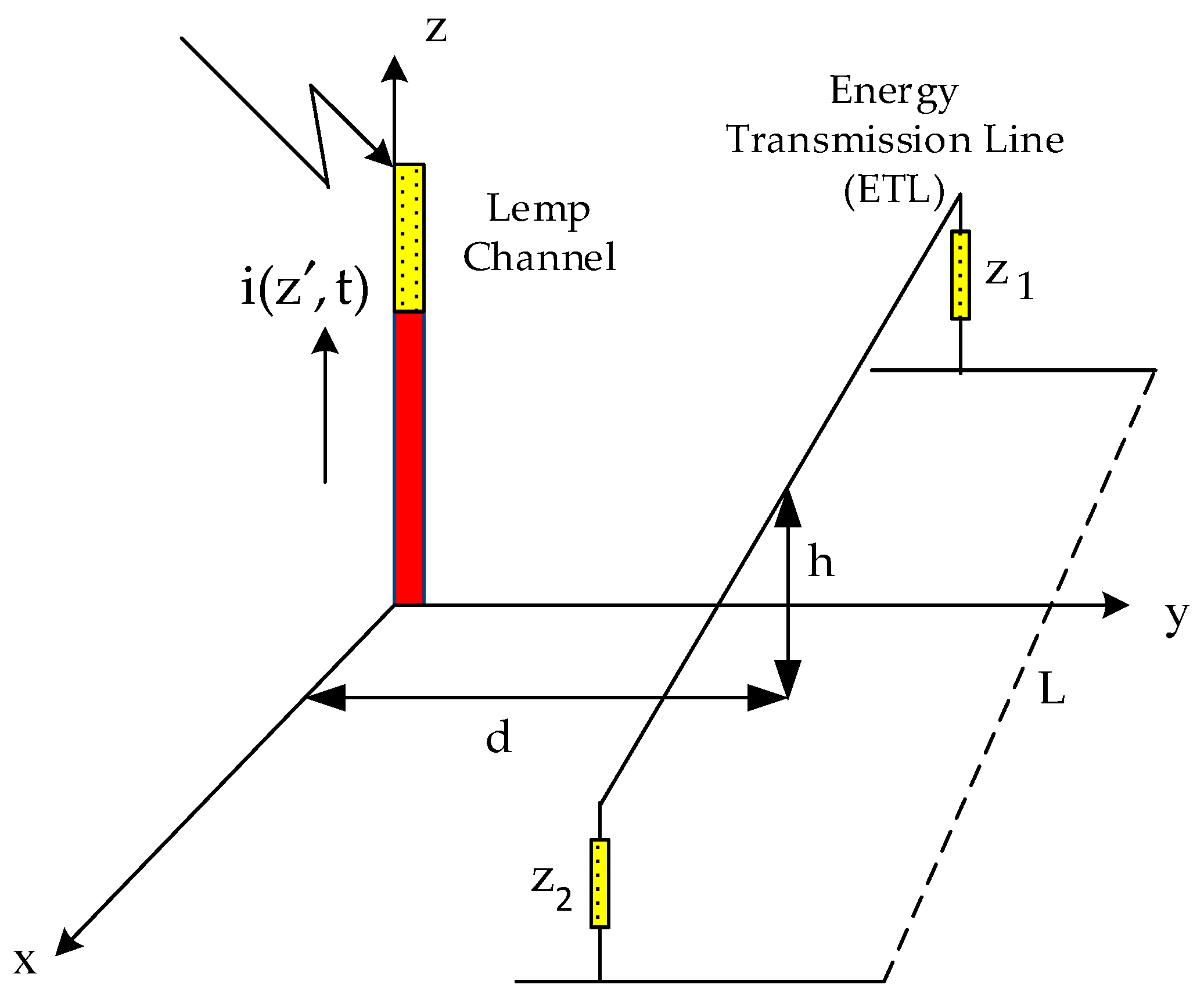
LEMP current models are divided into four classes. These models can be classified as gas dynamic models (or physics-based models), electromagnetic models, waveguide models, transmission line models and engineering models. Physical models are used for laboratory-designed simulations. Dynamic models are created based on air and variable environmental conditions. Due to their simplicity and ability to successfully reproduce prominent features of lightning electromagnetic pulses, feedback models belonging to the engineering model type are commonly used in practical applications. In this study, the Heidler model, which falls under engineering modeling, was utilized [19,20]. The Heidler current model was used as the LEMP flow model for this study. The LEMP reflected pulse pattern is shown in Figure 2.
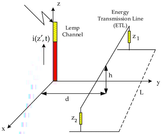
Figure 2.
Indirect drop of an LEMP on an exemplary ETL (d: the distance of the pulse from the line, h: the height of the transmission line, z1,2: the characteristic impedance of the transmission line pole).
Heidler Current Model
Heidler’s function is expressed in Equation (1) [21]:
The variables are as follows:
- : time constant of the rising current (s).
- : rot steady of the waveform of the rising current (s).
- n: specified steepness factor (between 2 and 10).
- : sufficiency esteem of the channel base current (A).
- u(t): unit step function.
- t: time (s).
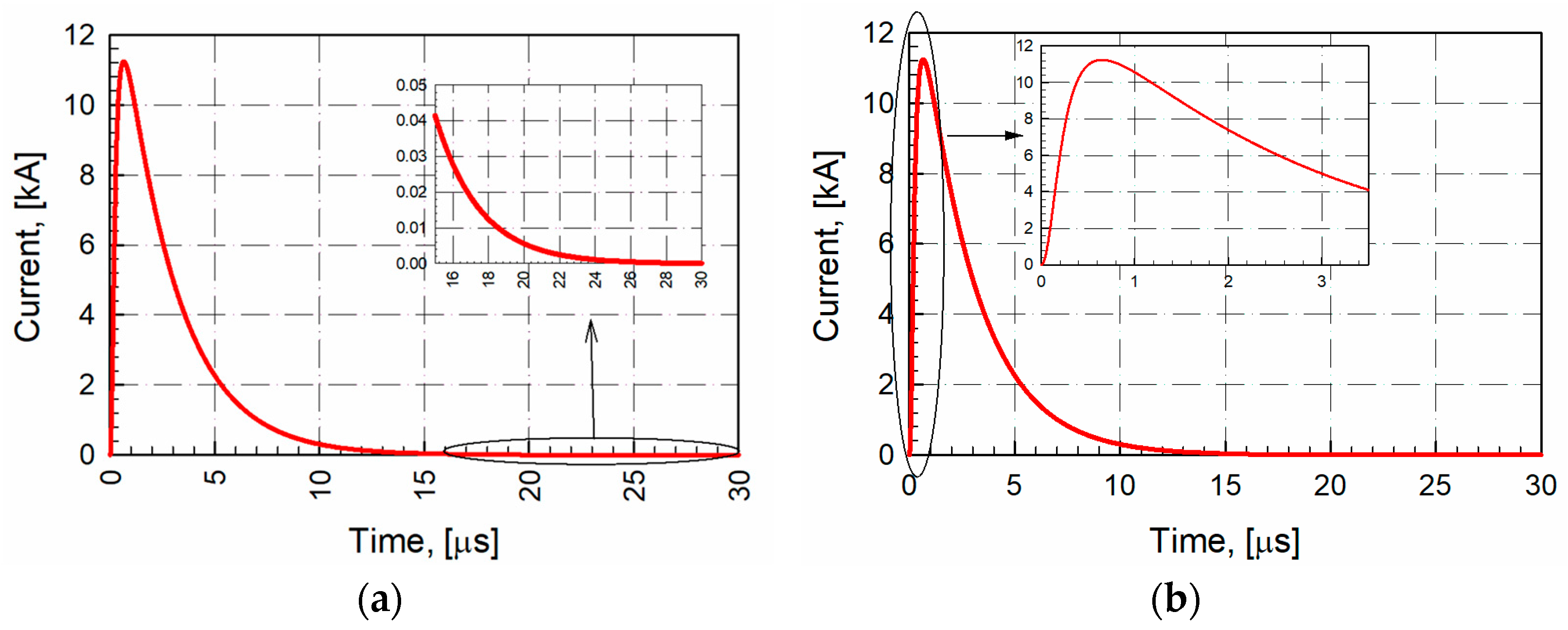
The LEMP form obtained by the Heidler current model is depicted in Figure 3a, with a detailed part denoted in Figure 3b. Figure 3a,b are derived mathematically [22]. Subsequent strokes can be modeled by varying the values of I0, τ1 and τ2 in the Heidler model. Two Heidler capacitors with specific parameters can be included to approximate the required current waveform. The advantage of the Heidler function is its ability to model a real lightning current more realistically because it closely approximates the characteristics of a real lightning strike.

Figure 3.
(a). The shape of the current form at the basis of the LEMP channel according to the Heidler model. (b). The flow formed at the base of the LEMP channel according to the Heidler flow model (detailed model).
2.4. LEMP Coupling Effect on ETLs
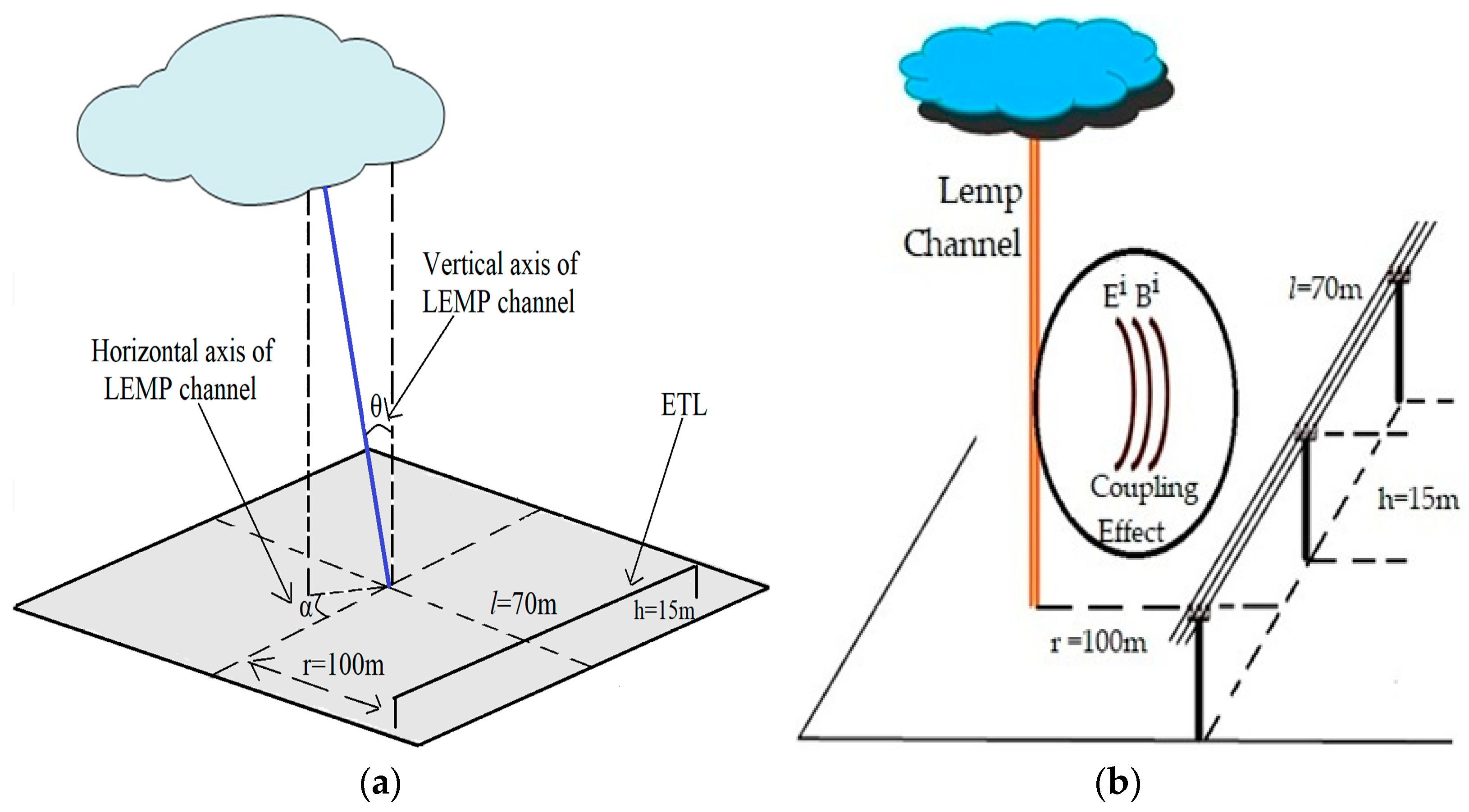
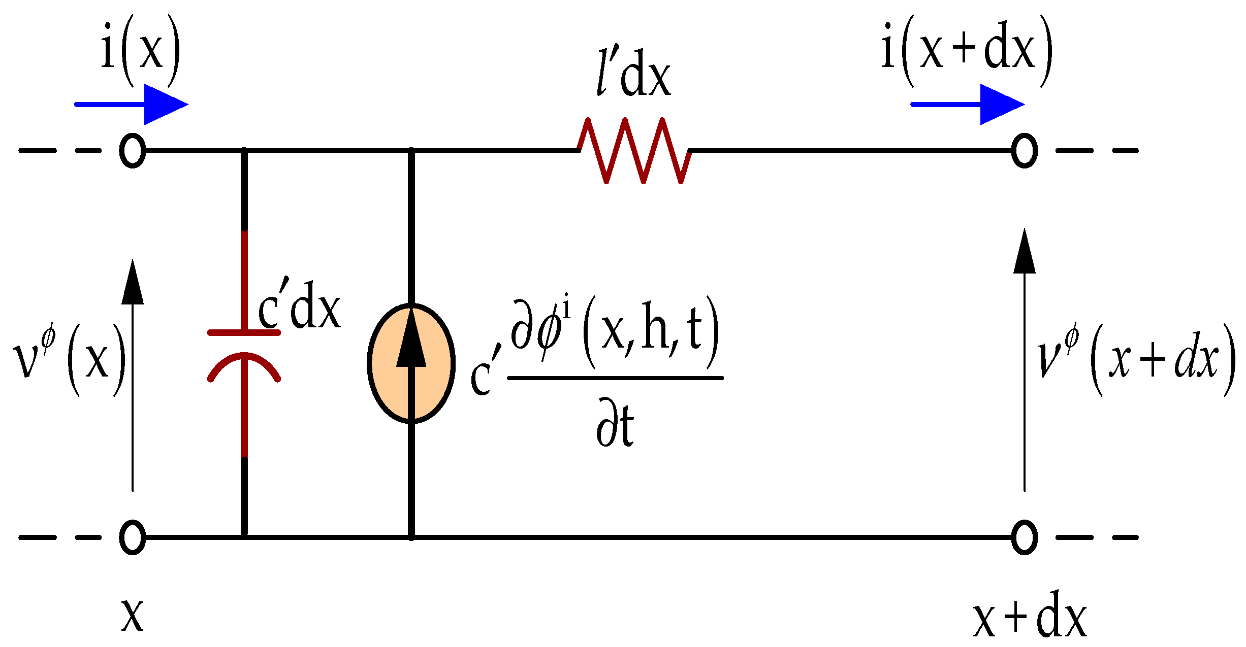
Electromagnetic fields are formed due to LEMP currents, and these fields can damage power grids [23]. Coupling between pulses and lines is achieved by utilizing different models of field line connections. Considering the geometry presented in Figure 4, these models are examined where the conductors are on perfectly conductive ground. Figure 5a,b illustrate how the coupling effect impacts the ETLs as a pair of electric and magnetic fields [23].
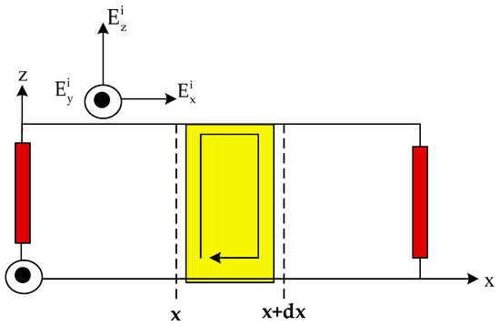
Figure 4.
Geometric structure of coupling models (: outward scattered electric field, dx: distance variation).

Figure 5.
(a). A geometric representation of the coupling effect of LEMPs on ETLs resulting from a specific angle (θ) of descent (top view, each part of the line is a spatial representation of our FDTD model) (b). Geometric representation of the coupling effect of LEMPs on ETLs (fall at right angles).
These models were utilized to predict LEMP-induced overvoltages in power lines, utilizing the Rusck closed formulation and the Rusck coupling model.
2.5. Rusck Closed Formulation and Rusck Coupling Model
The electromagnetic induction, coupling model, closed formulation, and field–ETL relationship evaluated by Rusck in the subtitles are depicted mathematically. The proposed closed-form solutions of the Rusck model are considered critical according to IEEE-1410 standards [24,25].
2.5.1. Rusck Coupling Model
Transmission line conditions related to the Rusck model are inferred by relating an electric field at the conductive surface with its conceivable outcomes. The corresponding power line coordination requirements given by Rusck are depicted through a combination of numerical conditions in Equations (2a,b) and (3) [23,26].
The variables are as follows:
- : the scalar potential in the transmission line near the region where the LEMP falls.
- : the total scalar potential generated by the LEMP current.
- t: the time constant.
The entire energized voltage u (x, t) on the line, where i (x, t) is the exact line current and L′ and C′ are the suitable inductance and capacitance on the line, is given as
In Equation (4a,b), h represents the height of the conductors, and Azi is the orthogonal component of the vector potential. The boundary conditions for conduction are given by Equation (4a,b), where t represents the time constant. (R0: space resistance, RL: line resistance.)
The closed formulation by Rusck was combined with the Heidler wave formulation, along with the boundary conditions, as shown in Equation (5). This combination resulted in more realistic results regarding the flow form by employing the Heidler current characteristic.
A simplified equation for LEMP-initiated overvoltage in an energy transmission line located in the region nearest the LEMP impact was proposed by Rusck. The related mathematical equation, denoted as Equation (6), is also presented [27]:
The variables are as follows:
- Vmax: maximum induced voltage (V).
- : dielectric constant of space (F/m).
- : magnetic permeability of the space (H/m).
- Z: characteristic impedance (Ω).
- : peak value of the LEMP current (A).
- d: distance of the LEMP drop location from the transmission line (m).
- v: speed of the LEMP (m/s).
- c: speed of light (m/s).
- h: height of the line from the ground (m).
Moreover, some restrictions should be applied when using Equation (7) only for perfect ground conductivity and a vertical LEMP channel for the ground. These restrictions are applied when the LEMP velocity is close to the velocity of light. Figure 6 shows the Rusck transmission line pattern [28]. The Rusck model mentioned above is superior to other coupling models and ignores the vector potential, focusing solely on the source-dependent portion of the even electric field. Despite this, the Rusck model correctly provides a coupling effect.

Figure 6.
A transmission line section represents the Rusck coupling model.
2.5.2. Rusck Formulation
Rusck illustrates the LEMP phenomenon with a vertical and straight channel, as shown in Figure 7. To explain the LEMP effect, a negative charge dissipates along the LEMP path before the return stroke begins. The return stroke may be a current surge within the framework of a step function that moves upward throughout the LEMP channel with a constant velocity, neutralizing the charge.

Figure 7.
The mathematical model of the LEMP according to the Rusck model. (v: the velocity of the pulse along the LEMP channel; the length of the initially loaded channel is limited and is expected to be (). h: the height of the line from the ground).
The Rusck return impact model is valid for a vertical and straight LEMP channel initially loaded with an evenly distributed load, as shown in Figure 7 [28]. The geometry of the problem for the evaluation of the area is depicted in Figure 8. The return stroke current is a step current that is spread along the channel in an undistorted and undiminished state. The expression portraying the current distribution for the model is shown in Equation (8).

Figure 8.
The geometry of the problem according to the Rusck formulation.
As it travels through the channel, the return current is initially charged with a favorable charge distribution, (), which neutralizes the negative charge distribution. The length of the initially loaded channel is limited and is expected to be (), the distance at any point in three-dimensional space (R) (Figure 8). The relationship between the current and charge distributions q0 is represented in Equation (9):
- is the scalar potential.
- defines the vector potential.
- β is the value related to the relative velocity.
- Γ is the Lorentz factor.
The potential created by the integral at the value of z = for the lower limit value s1 and the ground parameter z value is shown in Equation (13), and the solution for is depicted in Equation (14):
If the scalar potential formulation is rewritten after the solution, we obtain the solution presented in Equation (15):
The vector potential can be expressed as follows, given by Equations (13) and (16):
By substituting the general expression into the vector potential in Equation (12), it is also possible to acquire the vector potential’s vertical component, as denoted in Equation (17). Equation (18) expresses the magnetic field “B ()” and the electric field “E ()”.
According to the Rusck formulation, the electric field is divided into two parts. The first part is expressed as the scalar potential () and the vector potential ().
The ground produces two components of the electric field, which can be calculated using Equations (21) and (22) when z equals zero and is assumed to be on the ground axis:
If the magnetic field strength on the ground is expressed according to the Rusck formula, Equation (23) is obtained:
2.6. The Relationship between Fields and Lines According to Rusck Model
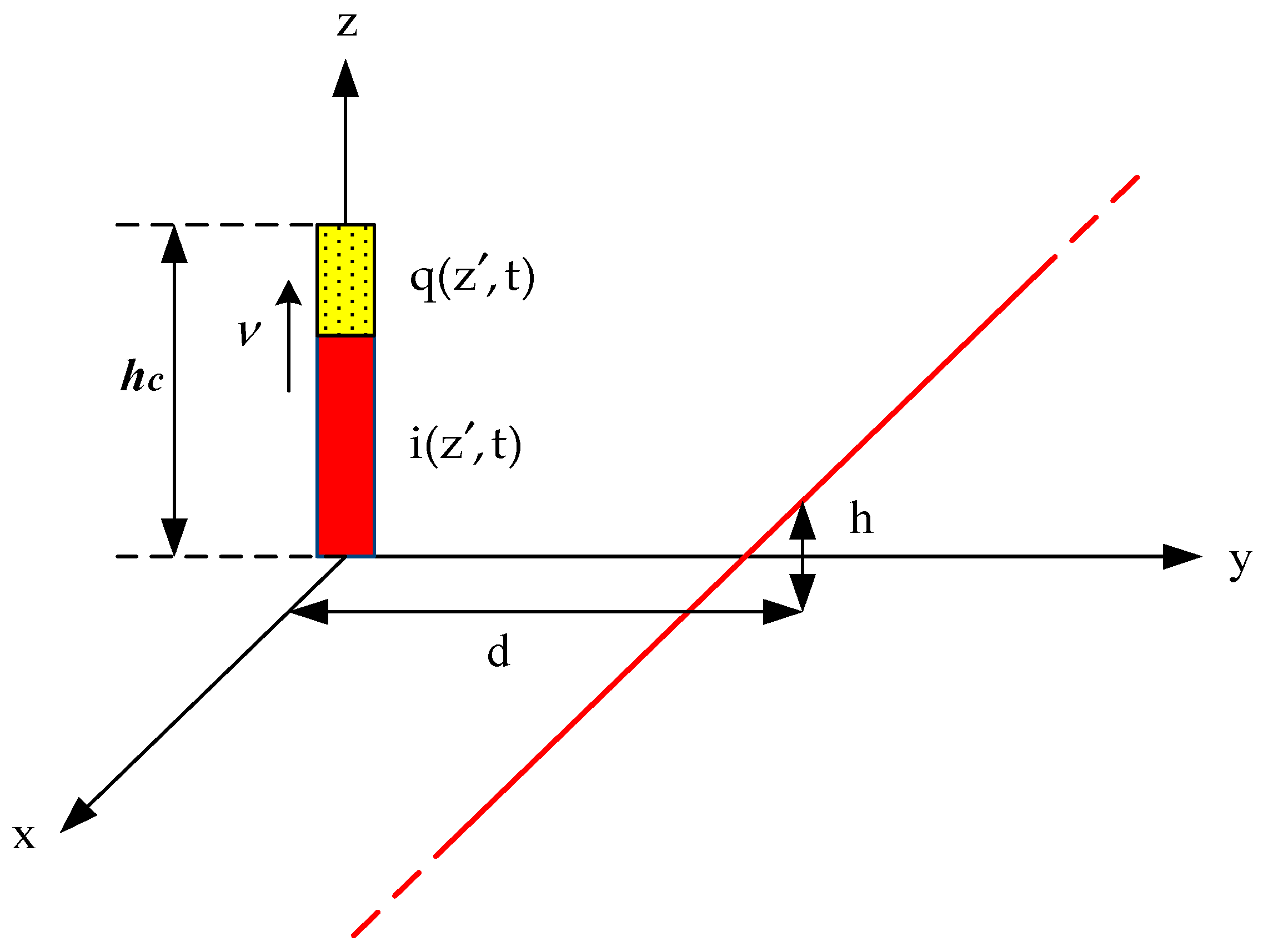
Rusck proposed a cable tying model based on the currents and voltages distributed along the line. The model’s equations relate the proposed transmission lines to the total electric field on the conductor surface, using scalar and vector potentials. The transmission line conditions determined by Rusck are expressed in Equation (24a,b), considering the geometry displayed in Figure 9 [29]:
The variables are as follows:
- : the scalar potential.
- l′: the line inductance, (H).
- c′: the line capacitance, (F).
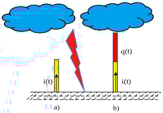
Figure 9.
(a). A straight and vertical LEMP current is moving upwards (no load model). (b). The negative charge is equitably disseminated along the LEMP; sometime recently, the return strike starts to account for the strike–strike of the driving shoot (loaded model). (i(t) time dependent variation of current, q(t) time dependent variation of the load).

The total voltage across the line is expressed as v (x, t) in Equation (25):
Figure 7 illustrates Rusck’s transmission line demonstration. The Rusck model assumes that the scalar and vector potentials between the electric field, ground and line height are constant and equal to the potentials on the ground surface. Rusck obtained equations based on these assumptions, which are expressed in Equations (26) and (27):
If (x = 0) is written to determine the voltage closest to the LEMP, Equation (27) is obtained:
2.7. Electric Field Change in the Initially Uncharged Channel of the LEMP Sprout
The electric field change was investigated when the LEMP sprout was uncharged and just before it fell to the ground. The unloaded state of the LEMP sprout is depicted in Figure 10. The equations used to analyze the problem are expressed by Equations (28)–(30). In these expressions, ‘ct’ denotes the distance traveled, ‘d’ is the line length, ‘x’ is the position of the LEMP channel concerning the degree of falling to the earth, δ is the time constant, and ‘Γ’ is the value of the Lorentz factor. shows the electric field formed in the uncharged channel [30,31,32].
2.8. Electric Field Change in the Initially Charged Channel of the LEMP Sprout
The electric field expression () is divided into two stages. In the first stage, the static electric field () is expressed, and in the other stage the dynamic electric field () is expressed. These two electric field expressions occur in the range of and are shown in Equation (31a,b):
The initial loading condition of the LEMP sprout is depicted in Figure 9a,b [33,34,35]. The equations used to calculate the change in the electric field for this state are expressed in Equations (32)–(34):
If the LEMP channel is initially loaded, Equations (32) and (33) are combined to obtain the main equation, as given in Equation (34):
3. Results
Analyses were performed using an electromagnetic field formulation based on accelerating charges instead of the traditional dipole approach. Thus, it was possible to obtain the final field expressions in a closed and compact form. The load-dependent component “(e)” was examined under the heading of the Rusck closed formulation and the coupling model, starting with a positive value, .
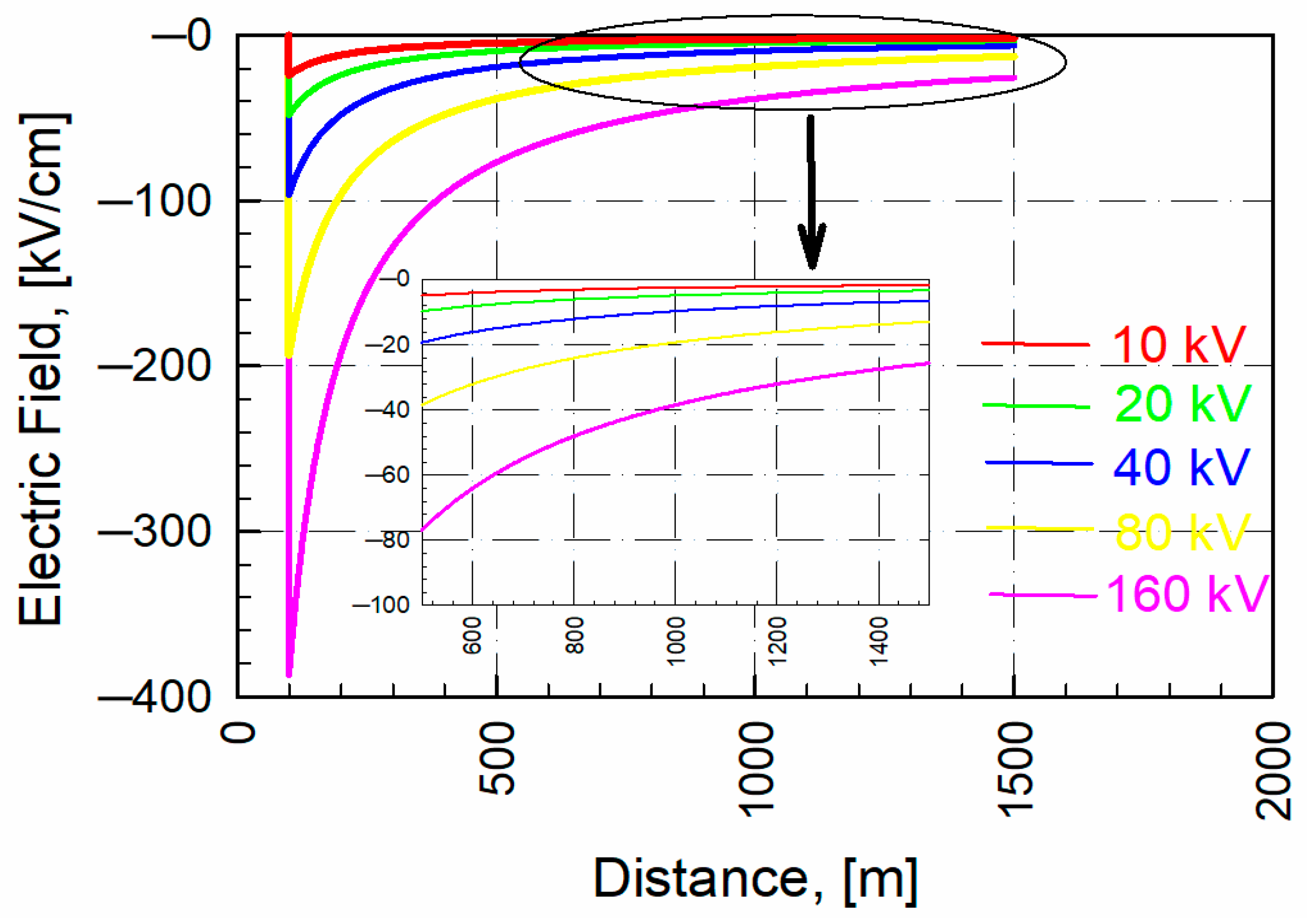
In Figure 10, the distance to the point where the LEMP falls according to different current values is determined as 100 m from the transmission line. The reason for choosing this value is to ensure that the pulse is close to the power transmission lines. The vertical electric field value formed at the foundation of the overhead line at this distance is shown in Figure 11. This value drops to zero when the return pulse approaches the cloud. The eA component due to the LEMP current starts to increase from zero. Initial values are obtained if the t = r/c equation is written instead of t in the equations in Equations (21) and (22). In Figure 11 and Figure 12, , eA and are analyzed and represented analytically.
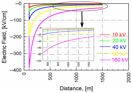
Figure 11.
Vectorial component for different LEMP currents for r = 100 m and z = 0 depending on the load distribution along the LEMP channel. (Solution for the function in Equation (22)).

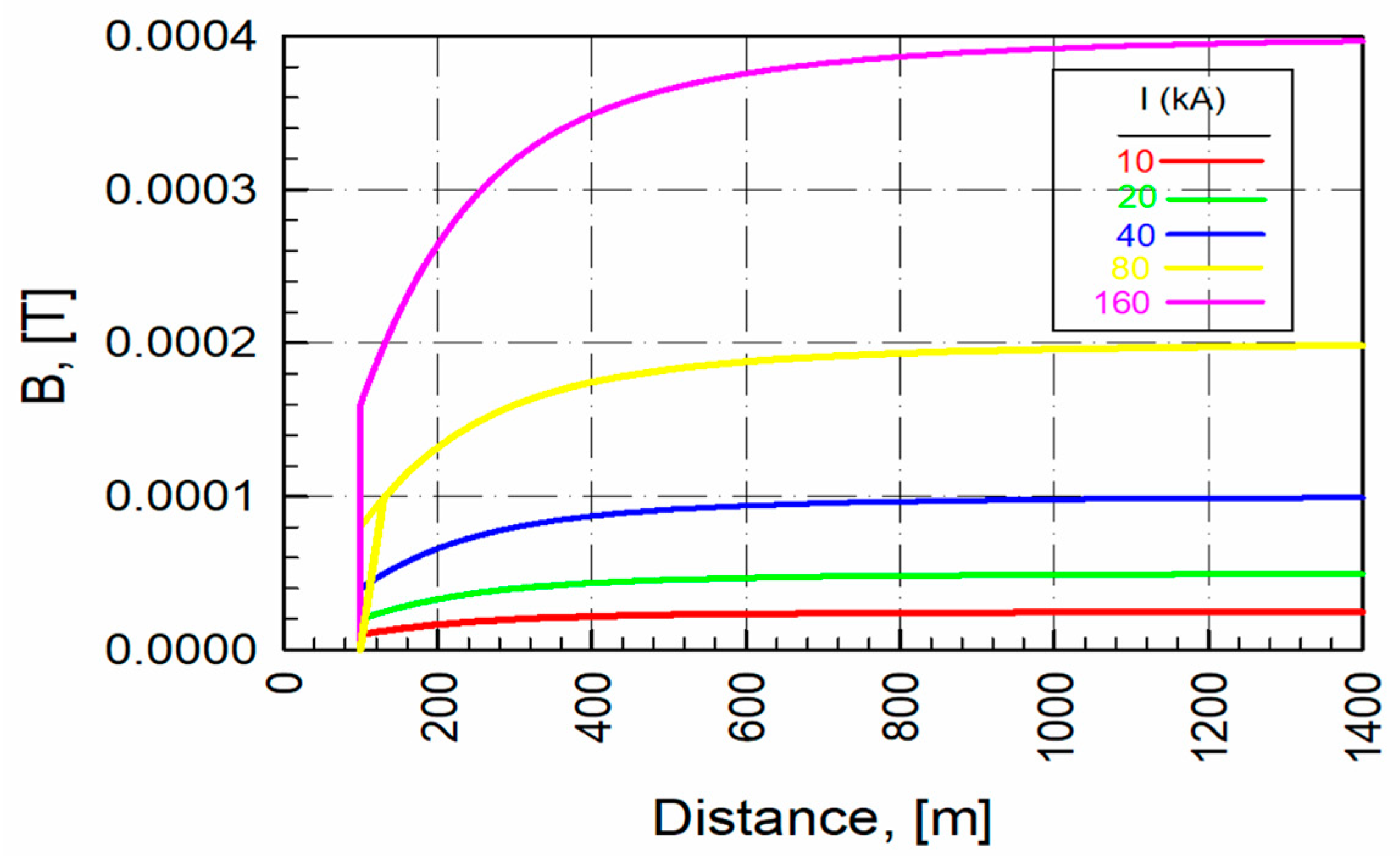
Figure 12.
Magnetic field component for different LEMP currents for r = 100 m and z = 0 depending on the load distribution along the LEMP channel. (Solution for the function in Equation (23)).
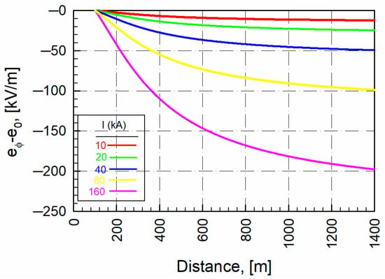
Figure 10.
The vertical electric field and scalar component for different LEMP currents for r = 100 m and z = 0 depending on the load distribution throughout the LEMP channel (solution for the function in Equations (21) and (22)).
Figure 10.
The vertical electric field and scalar component for different LEMP currents for r = 100 m and z = 0 depending on the load distribution throughout the LEMP channel (solution for the function in Equations (21) and (22)).
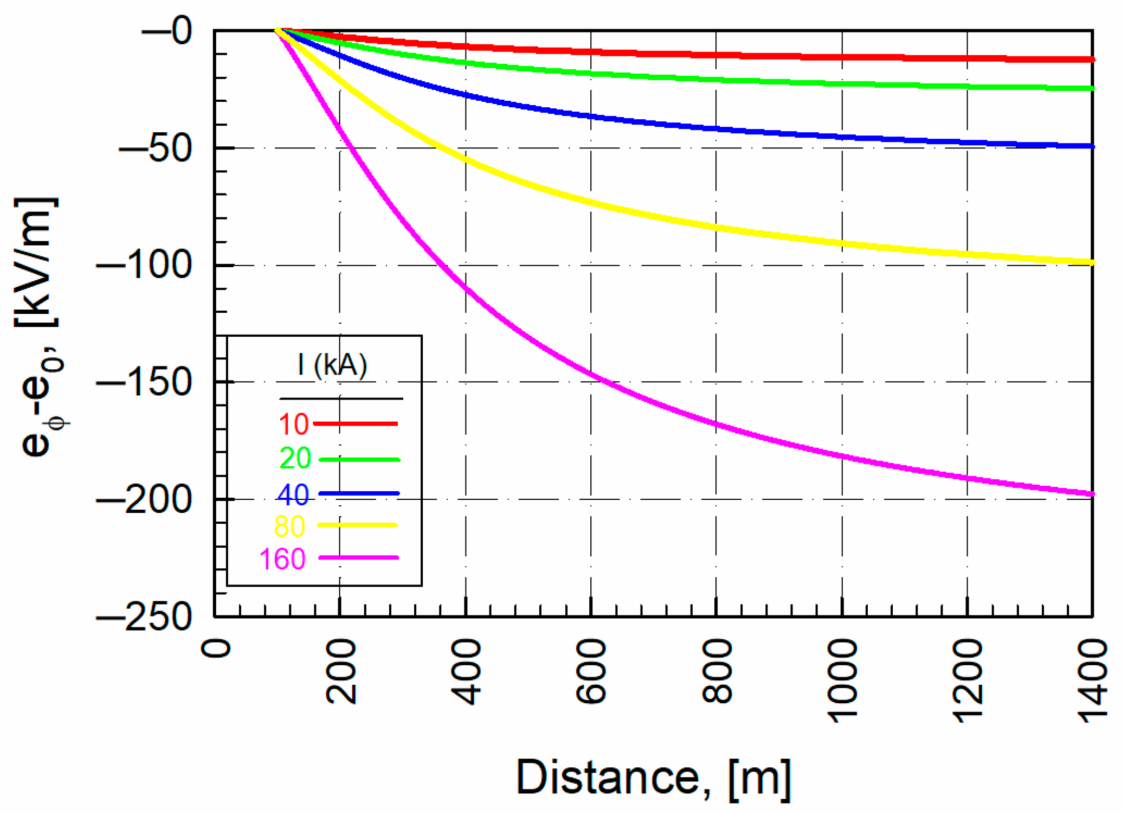
In Figure 11, the vector components of the electric field formed at the base of the overhead line located 100 m away from the point where the LEMP fell are shown for different current values. In Figure 12, the magnetic field values for the same configuration are denoted. If the equation “” is placed in Equation (26), the Vpeak value is obtained.
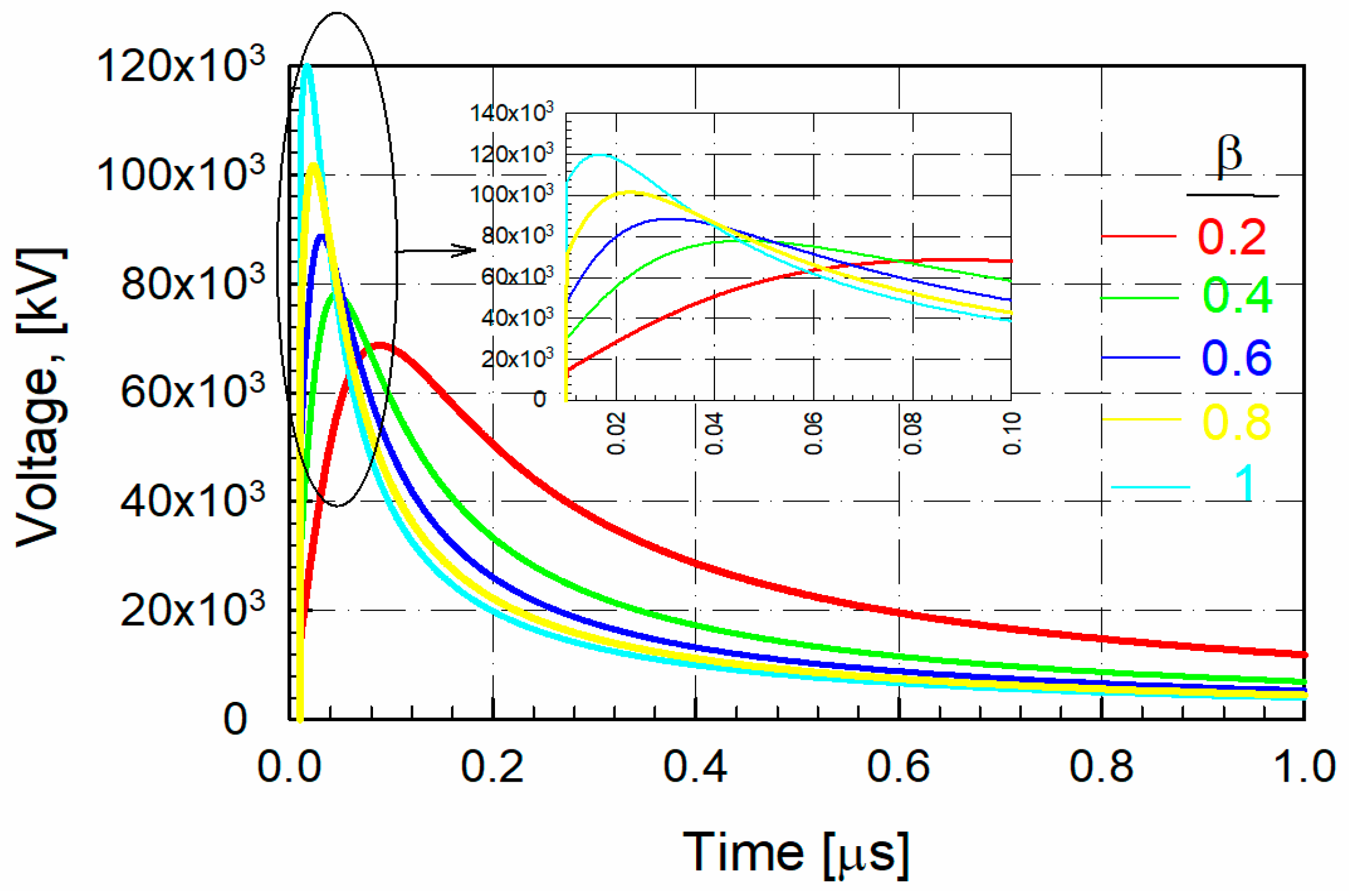
“” indicates the peak value of the induced stress recommended by IEEE standard 1410 [36,37]. Here, the β value indicates the relative velocity. Similarly, the actuation voltage was obtained from a line 15 m tall and 70 m away from the point where the LEMP fell Figure 13. The distance between two transmission poles, d = 70 m, is defined. The values were chosen because Turkish transmission systems typically use a distance between 40 and 70 m. This falls within the range of 15–40 m commonly used in Turkish transmission systems. The height of the pole, h = 15 m, is also defined. The lowest value was chosen to better understand the effect of the indirect pulse on the transmission line. The voltages concerning different β values (relative speed) were obtained for an LEMP current of 15 kA.
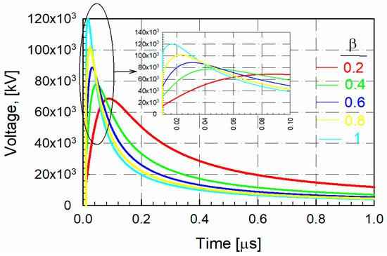
Figure 13.
Induced voltage graph at x = 0 according to Rusck’s formula. The voltage was induced on a line at a distance of 70 m from the LEMP sprout and at the height of 15 m for = 15 kA. (Solution for the function in Equation (27)).
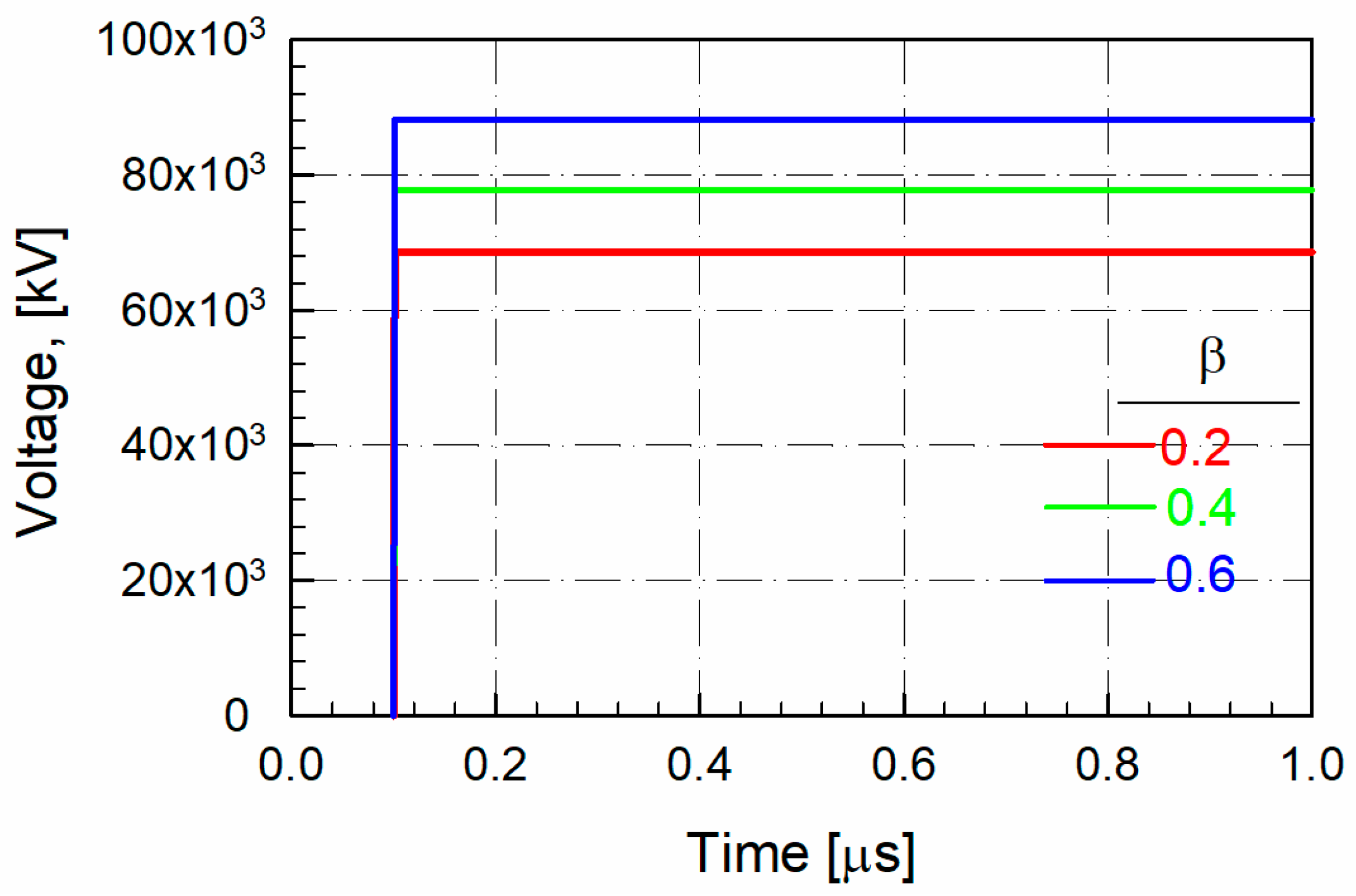
In Figure 14, the peak value of the induced voltage according to the relative velocity is detailed. In particular, the validity of the model underlying the solutions and the approaches used in this model were analyzed, and the results in the literature were confirmed. The speed of the LEMP sprout affected the induced overvoltage value and the waveform, especially at the anterior slope of the wave. It was determined that the highest possible value of overvoltage induced in places far from the point where LEMP falls is proportional to the velocity of the LEMP sprout. Additionally, it is observed in Figure 14 that the speed has no effect at t = 0 on the induced overvoltage at a place near the impact point.

Figure 14.
The voltage values induced at x = 0 according to the Rusck equation. Detailed view of the peak value of the induced voltage on a line at the height of 10 m and at a distance of 50 m from the point where the LEMP sprout fell concerning its relative velocity for = 10 kA (solution for the function in Equation (27)).
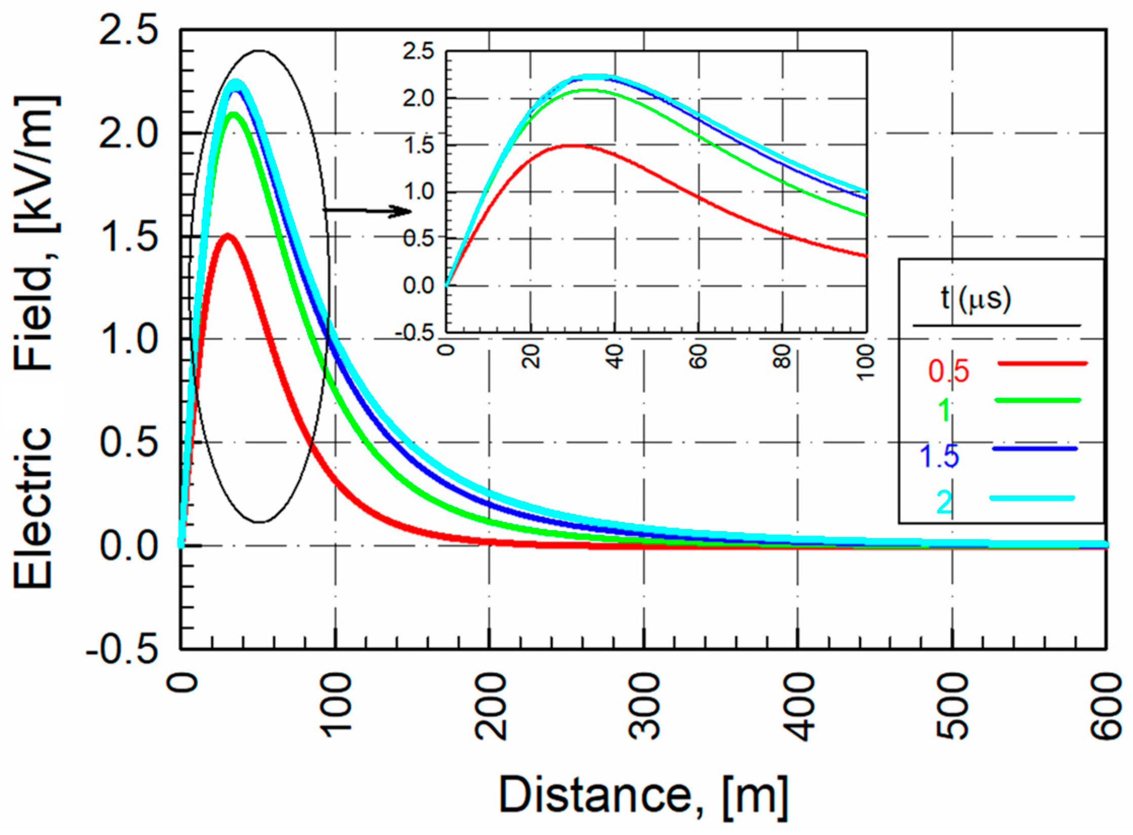
This study examined the change in the electric field in the initially uncharged channel of the LEMP sprout using Equation (29), and we present the findings in Figure 15. This paper also discusses the event of an initial charge using Equation (33) and presents the results in Figure 16. Since the analytical equivalence of the two LEMP events is determined Figure 10, the result of this study is significant.
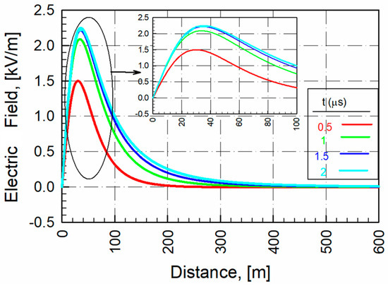
Figure 15.
Electric field change (x = 0, = 15 kA, β = 0.4, h = 15 m, and d = 70 m) when the LEMP channel is initially uncharged. (Solution for the function in Equation (31a)).
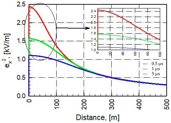
Figure 16.
Electric field change (x = 0, = 15 kA, β = 0.4, h = 15 m, and d = 70 m) when the LEMP channel is initially loaded. (Solution for the function in Equation (34)).
4. Discussion and Conclusions
This study examined the impact of transient events on power transmission lines and power plants by creating LEMP offshoots using Heidler and Rusck functions. In Rusck’s field-to-line coupling model, the electric field used in the coupling equations is derived from expressions of Rusck’s model for the electric field of a return stroke current propagating at a constant velocity along a vertical channel [28]. The effect of the indirect fall (discharge) of the LEMP sprout on the nearby ETLs was analyzed in the first analysis. Different drop currents of the LEMP sprout were used to obtain the vertical electric field generated by the dispersed charge from the LEMP. This study revealed that an increase in the current of the LEMP leads to an increase in the value of the vertical electric field and the induced voltage. Specifically, the electric field value generated by a 160 kA LEMP at the base of an overhead line 100 m away was −3.87 kV/m. Additionally, an LEMP of the same magnitude produced a scalar value of 200 kV/m at 1.5 ms at the base of an overhead line 100 m away, depending on the time. This finding supports Aigner’s suggestion. Furthermore, the vector component of the vertical electric field was examined for various LEMP current levels. Unlike previous studies in the literature, this study investigates both the vector and scalar components of the vertical electric field for different LEMP values. It was observed that the scalar component (200 kV/m at 100 m away for the same current value) is more destructive than the vector component (−3.87 kV/m at 100 m away). This study also obtained the magnetic field values generated by the LEMP at different falling current values. The analysis revealed that the magnetic field value in the region where the falling current of the LEMP sprout increases also increases non-linearly. Specifically, a 160 kA LEMP creates a magnetic field intensity of 0.4 mT at the foundation of the overhead line 100 m away in 1.5 ms [38].
It was found that the increase in the propagation speed of LEMP sprouts is directly proportional to the gains in the induced voltage in ETLs and power plants as they approach the speed of light. To prevent this issue, the grounding foundations of the poles on certain lines should be shielded where lightning strikes are most frequent. This will improve electromagnetic compatibility and reduce the risk of indirect impacts. This study analyzed the transient voltage values that arise in ETLs and energy facilities based on the propagation speed of LEMP sprouts, according to the area–line relationship. The results showed that the voltage induced in ETLs and power equipment increases in direct proportion to the speed of propagation of the LEMPs as they approach the speed of light.
Furthermore, this study examined the effectiveness of LEMPs in the forward trend of the wave and the electrical conditions they create in the region before falling to the ground. This study looked at the humidity levels in the region where the LEMP sprout fell to the ground, as well as the electrical conditions in high-altitude regions. As the formation time of the LEMP sprout approached, the electric field value increased. Specifically, the electric field value produced by the 15 kA LEMP at 0.5 µs in the conductors on the 15 m high pole of the overhead line, which was 70 m away from the point where the channel fell before the channel was formed, was measured as 1.5 kV/m [39]. The fall location of the LEMP sprout can be predicted by selecting electric field values in specific lines within the regions most exposed to LEMPs. Furthermore, the electric field value was analyzed based on the time and distance from the point of impact after the LEMP discharge occurred. It was concluded that the electric field value decreased as the damping time and distance increased. After forming the channel of the 15 kA LEMP sprout, the electric field value created in 0.5 µs in the conductors located on the 15 m high pole of the overhead line 70 m away was determined to be 2.4 kV/m. It was observed that the effect on the line disappears over time. The electric field produced on the pole of the line 500 m away by moving in the shape of a traveling wave on the same line was calculated to be 0.3 kV/m. The results support Bewley’s perspective on the matter and clarify the indirect coupling effects of LEMPs on energy transmission lines and facilities. The combination of the Rusck approach and the Heidler wave equation can be used to evaluate the indirect LEMP performance of overhead power lines with high accuracy, thereby avoiding significant losses of accuracy. This study is unique from other studies in the literature as it utilizes electromagnetic field functions based on accelerating loads rather than the traditional dipole approximation, thus presenting graphical results that do not require interpolation. LEMPs are a complex natural phenomenon. The more realistically we can model this impulse mathematically, the better we can prevent transient damage to electrical facilities. These models will facilitate the pre-determination of surge current values to protect energy transmission lines exposed to LEMPs, thus aiding in the selection of appropriate levels for protective devices. Additionally, we believe that these mathematical models will gain importance in harnessing the energy of LEMPs in future studies.
Author Contributions
Conceptualization, T.C., H.F.C. and S.O.; methodology, T.C., H.F.C. and S.O.; software T.C., H.F.C. and S.O.; validation, T.C., H.F.C. and S.O.; formal analysis, T.C., H.F.C. and S.O.; investigation, T.C., H.F.C. and S.O.; resources, T.C., H.F.C. and S.O.; data curation, T.C., H.F.C. and S.O.; writing—original draft preparation, T.C., H.F.C. and S.O.; writing—review and editing, T.C., H.F.C. and S.O.; visualization, T.C., H.F.C. and S.O.; supervision, T.C., H.F.C. and S.O.; project administration, T.C., H.F.C. and S.O.; funding acquisition, T.C., H.F.C. and S.O. All authors have read and agreed to the published version of the manuscript.
Funding
This research received no external funding.
Informed Consent Statement
Not applicable.
Data Availability Statement
The raw data supporting the conclusions of this article will be made available by the authors on request.
Conflicts of Interest
The authors declare no conflict of interest.
References
- Wagner, K.W. Elektromagnetische Ausgleichs Vorgange in Freileitungen und Kabeln; Electromagnetic and Acoustical Scattering by Simple Shapes; Teubner: Berlin, Germany, 1908; Volume 5. [Google Scholar]
- Bewley, L.W. Traveling Waves due to lightning. AIEE Trans. 1929, 48, 1050–1064. [Google Scholar] [CrossRef]
- Aigner, V. Induzierte Blitzuberspannunen und Ihre Bezie-Hung Zum Ruck Wertigen; Überschlag ETZ: Berlin, Germany, 1935; pp. 497–500. [Google Scholar]
- Szpor, S. A New Theory of the Induced over Voltages; Cigré Report; CIGRE: Paris, France, 1948; p. 308. [Google Scholar]
- Rusck, S. Induced Lightning Over-Voltages on Power Transmission Lines with Special Reference to the Overvoltage Protection of Low-Voltage Networks; Elanders Boktryckeri Aktiebolag: Stockholm, Sweden, 1958. [Google Scholar]
- IEEE Std 1410-2004; IEEE Guide for Improving the Lightning Performance of Electric Power Overhead Distribution. IEEE: Piscataway, NJ, USA, 2004.
- Andreotti, A.; Pierno, A.; Rakov, V.A.; Verolino, L. Analytical Formulations for Lightning-Induced Voltage Calculations. IEEE Trans. Electromagn. Compat. 2013, 55, 109–123. [Google Scholar] [CrossRef]
- Cooray, V.; Cooray, G.; Rubinstein, M.; Rachidi, F. Exact Expressions for Lightning Electromagnetic Fields: Application to the Rusck Field-to-Transmission Line Coupling Model. Atmosphere 2023, 14, 350. [Google Scholar] [CrossRef]
- Nematollahi, A.F.; Vahidi, B. The effect of the inclined lightning channel on electromagnetic fields. Electr. Eng. 2021, 103, 3163–3176. [Google Scholar] [CrossRef]
- Mahmood, F.; Rizk, M.E.M.; Lehtonen, M. Risk-based insulation coordination studies for protection of medium-voltage overhead lines against lightning-induced overvoltages. Electr. Eng. 2019, 101, 311–320. [Google Scholar] [CrossRef]
- Ates, K.; Carlak, H.F.; Ozen, S. Dosimetry analysis of the magnetic field of underground power cables and magnetic field mitigation using an electromagnetic shielding technique. Int. J. Occup. Saf. Ergon. 2022, 28, 1672–1682. [Google Scholar] [CrossRef] [PubMed]
- Lakhdar, A. Numerical Simulation of the Negative Downward Leader Current with the Associated Far-EM Field Generated by Lightning. IEEE Trans. Electromagn. Compat. 2024, 66, 240–246. [Google Scholar] [CrossRef]
- Nicolae, P.-M.T.; Nicolae, I.-D.V.D.; Nitu, M.-C.; Nicolae, M.-S.P.M. Analysis and Experiments Concerning Surges Transferred Between Power Transformer Windings Due to Lightning Impulse. IEEE Trans. Electromagn. Compat. 2023, 65, 1476–1483. [Google Scholar] [CrossRef]
- Rizk, M.E.M.; Ghanem, A.; Abulanwar, S.; Shahin, A.; Baba, Y.; Mahmood, F.; Ismael, I. Induced Electromagnetic Fields on Underground Cable Due to Lightning-Struck Wind Tower. IEEE Trans. Electromagn. Compat. 2023, 65, 1684–1694. [Google Scholar] [CrossRef]
- Koike, S.; Baba, Y.; Tsuboi, T.; Rakov, V.A. Lightning Current Waveforms Inferred from Far-Field Waveforms for the Case of Strikes to Tall Objects. IEEE Trans. Electromagn. Compat. 2023, 65, 1162–1169. [Google Scholar] [CrossRef]
- Ain, N.U.; Andreotti, A.; Mahmood, F.; Rizk, M.E.M. A Correction to Rusck Expression for the Evaluation of Lightning-Induced Overvoltages for High-Resistivity Ground. IEEE Trans. Electromagn. Compat. 2023, 65, 1152–1161. [Google Scholar] [CrossRef]
- Tatematsu, A.; Yamanaka, A. Three-Dimensional FDTD-Based Simulation of Lightning-Induced Surges in Secondary Circuits with Shielded Control Cables Over Grounding Grids in Substations. IEEE Trans. Electromagn. Compat. 2023, 65, 528–538. [Google Scholar] [CrossRef]
- Viscaro, S. Direct Strokes to Transmission Lines: Considerations on the mechanisms of Overvoltage Formation and their Influence on the Lightning Performance of Lines. J. Light. Res. 2007, 1, 60–68. [Google Scholar]
- Master, M.J.; Uman, M.A.; Lin, Y.T.; Standler, R.B. Calculations of lightning return stroke electric and magnetic fields above ground. J. Geophys. Res. 1981, 86, 127–132. [Google Scholar] [CrossRef]
- Diendorfer, G.; Uman, M.A. An improved return stroke model with specified channel-base current. J. Geophys. Res. 1990, 95, 13621–13644. [Google Scholar] [CrossRef]
- Heidler, F. Travelling current source model for LEMP calculation. In Proceedings of the 6th Symposium and Technical Exhibition on Electromagnetic Compatibility, Zurich, Switzerland, 5–7 March 1985. [Google Scholar]
- Nucci, C.A.; Rachidi, F.; Ianoz, M.; Mazzetti, C. Comparison of Two Coupling Models for Lightning-Induced Over-voltage Calculations. IEEE Trans. Power Deliv. 1995, 10, 330–339. [Google Scholar] [CrossRef]
- Montano, R. The Effects of Lightning on Low Voltage Power Networks. Ph.D. Thesis, Uppsala University, Uppsala, Sweden, 2005. [Google Scholar]
- Barker, P.P.; Short, T.A.; Eybert-Berard, A.R.; Berlandis, J.P. Induced voltage measurement on an experimental distribution line during nearby rocket triggered lightning flashes. IEEE Trans. Power Deliv. 1996, 11, 980–995. [Google Scholar] [CrossRef]
- Nucci, C.A.; Rachidi, F.; Ianoz, M.V.; Mazzetti, C. Lightning Induced Voltages on Overhead Power Lines. IEEE Trans. Electromagn. Compat. 1993, 35, 75–86. [Google Scholar] [CrossRef]
- Darveniza, M. A Practical Extension of Rusck’s Formula for Maximum Lightning-Induced Voltages That Accounts for Ground Resistivity. IEEE Trans. Power Deliv. 2007, 22, 605–612. [Google Scholar] [CrossRef]
- Rusck, S.; Golde, R.H. Protection of Distribution Lines in Lightning; Academic Press: London, UK, 1977; Volume 2, pp. 747–771. [Google Scholar]
- Cakil, T. Investigation of The Effects of Lightning Electromagnetic Structures on High Voltage Electrical Facilities. Master’s Thesis, Akdeniz University, Antalya, Turkey, 2017. [Google Scholar]
- Cooray, V. Calculating lightning-induced over voltages in power lines. A comparison of two coupling models. IEEE Trans. Electromagn. Compat. 1994, 36, 179–182. [Google Scholar] [CrossRef]
- Hoidalen, H. Analytical Formulation of Lightning-Induced Voltages on Multiconductor Overhead Lines Above Lossy Ground. IEEE Trans. Electromagn. Compat. 2003, 45, 92–100. [Google Scholar] [CrossRef]
- Liew, A.C.; Mar, S.C. Extension of the Chowdhuri—Gross Model for Lightning Induced Voltage on Overhead Lines. IEEE Trans. Power Syst. 1986, 1, 240–247. [Google Scholar] [CrossRef]
- Rachidi, F.; Nucci, C.A.; Ianoz, M. Transient Analysis of Multiconductor Lines Above a Lossy Ground. IEEE Trans. Power Deliv. 1999, 14, 294–302. [Google Scholar] [CrossRef]
- Cakil, T.; Carlak, H.F.; Ozen, S. The Analysis of Transient Phenomena on Power Transmission Lines Due to Lightning Electromagnetic Pulses. In Proceedings of the 2017 Progress in Electromagnetics Research Symposium—Spring (PIERS), St. Petersburg, Russia, 22–25 May 2017. [Google Scholar]
- Cooray, V. The Lightning Flash; Institution of Electrical Engineers: London, UK, 2003. [Google Scholar]
- Borghetti, A.; Nucci, C.A.; Paolone, M.; Rachidi, F. Characterization of the response of an overhead distribution line to lightning electromagnetic fields. In Proceedings of the ICLP 2000, 25th International Conference on Lightning Protection, Rhodes, Greece, 18–22 September 2000. [Google Scholar]
- Nucci, C.A. Lightning-Induced Voltages on Overhead Power Lines. Part II: Coupling Models for the Evaluation of the Induced Voltages. Electra 1995, 162, 121–145. [Google Scholar]
- Ishimoto, K.; Tossani, F.; Napolitano, F.; Borghetti, A.; Nucci, C.A. LEMP and ground conductivity impact on the direct lightning performance of a medium-voltage line. Electr. Power Syst. Res. 2023, 214, 108845. [Google Scholar] [CrossRef]
- Delfino, F.; Procopio, R.; Andreotti, A.; Verolino, L. Lightning return stroke current identification via field measurements. Electr. Eng. 2002, 84, 41–50. [Google Scholar] [CrossRef]
- Helhel, S.; Ozen, S. Assessment of occupational exposure to magnetic fields in high-voltage substations (154/34.5 kV). Radiat. Prot. Dosim. 2008, 128, 464–470. [Google Scholar] [CrossRef] [PubMed]


Disclaimer/Publisher’s Note: The statements, opinions and data contained in all publications are solely those of the individual author(s) and contributor(s) and not of MDPI and/or the editor(s). MDPI and/or the editor(s) disclaim responsibility for any injury to people or property resulting from any ideas, methods, instructions or products referred to in the content. |
© 2024 by the authors. Licensee MDPI, Basel, Switzerland. This article is an open access article distributed under the terms and conditions of the Creative Commons Attribution (CC BY) license (https://creativecommons.org/licenses/by/4.0/).