Article

A Method for Underwater Biological Detection Based on Improved YOLOXs

School of Mathematics and Computer Science, Wuhan Polytechnic University, Wuhan 430048, China
*
Author to whom correspondence should be addressed.
Appl. Sci. 2024, 14(8), 3196; https://doi.org/10.3390/app14083196
Submission received: 31 January 2024 / Revised: 28 March 2024 / Accepted: 2 April 2024 / Published: 10 April 2024

Abstract

:
This article proposes a lightweight underwater biological target detection network based on the improvement of YOLOXs, addressing the challenges of complex and dynamic underwater environments, limited memory in underwater devices, and constrained computational capabilities. Firstly, in the backbone network, GhostConv and GhostBottleneck are introduced to replace standard convolutions and the Bottleneck1 structure in CSPBottleneck_1, significantly reducing the model’s parameter count and computational load, facilitating the construction of a lightweight network. Next, in the feature fusion network, a Contextual Transformer block replaces the 3 × 3 convolution in CSPBottleneck_2. This enhances self-attention learning by leveraging the rich context between input keys, improving the model’s representational capacity. Finally, the positioning loss function Focal_EIoU Loss is employed to replace IoU Loss, enhancing the model’s robustness and generalization ability, leading to faster and more accurate convergence during training. Our experimental results demonstrate that compared to the YOLOXs model, the proposed YOLOXs-GCE achieves a 1.1% improvement in mAP value, while reducing parameters by 24.47%, the computational load by 26.39%, and the model size by 23.87%. This effectively enhances the detection performance of the model, making it suitable for complex and dynamic underwater environments, as well as underwater devices with limited memory. The model meets the requirements of underwater target detection tasks.

1. Introduction

With the rapid development of social and economic activities, global issues such as the scarcity of terrestrial resources and environmental degradation have become increasingly prominent. In pursuit of sustainable human development, the exploration and utilization of marine resources have become a focal point of attention. Oceans cover the vast majority of the Earth’s surface and harbor abundant resources, including petroleum, natural gas, minerals, and fisheries [1]. At the same time, the oceans harbor diverse ecosystems and serve as habitats for numerous species. Therefore, the proper development and utilization of marine resources can not only meet human demands for energy, food, and raw materials but also protect the integrity of marine ecosystems and ensure sustainable development. In this context, many coastal countries are actively engaged in the exploration and exploitation of marine resources. Through technological innovation and cooperation, they are seeking and developing deep-sea oil and gas resources, conducting exploration and exploitation of seabed minerals, and promoting the sustainable development of fisheries.
In the process of marine resource development and utilization, underwater target detection is a crucial area of research in marine technology. Traditional underwater target detection techniques primarily involve manually designed feature extraction from images [2], followed by the use of machine learning algorithms for target classification [3]. While this approach can achieve underwater target detection to some extent, it has drawbacks in the feature extraction stage. Manual feature extraction incurs significant labor and time costs, and the features that are extracted manually may have limitations, such as being relatively simple and lacking strong generalization capabilities. To address these challenges, there is a need for advanced methods that leverage modern computer vision and deep learning techniques to enhance underwater target detection. These approaches can automate the feature extraction process, reducing human intervention and improving the overall efficiency and effectiveness of underwater target detection in complex marine environments.
To address these challenges, underwater target detection techniques based on deep learning have emerged [4,5]. Deep learning-based methods leverage deep neural networks to automatically learn features, including more abstract and advanced feature representations. Through extensive training with large amounts of data, these models acquire better generalization capabilities, enabling end-to-end underwater target detection. In recent years, deep learning-based underwater target detection techniques have made significant progress and can be categorized into two-stage and one-stage target detection algorithms. Two-stage target detection algorithms first generate a series of candidate boxes as samples and then use convolutional neural networks for sample classification. Examples of two-stage algorithms include R-CNN [6], FastR-CNN [7], FasterRCNN [8], and Cascade R-CNN [9], among others. On the other hand, one-stage target detection algorithms do not need to generate candidate boxes; they only need to input the image once to predict all the bounding boxes and classifications. This approach is characterized by its simple structure and fast processing speed. Examples of one-stage algorithms include SSD [10] and the YOLO (You Only Look Once) series [11,12,13,14,15].
With increasing underwater exploration activities, more scholars are applying target detection techniques to underwater environments. In 2019, Moniruzzaman et al. applied FastRCNN to underwater seagrass target detection [16]. They used data augmentation to generate more diverse training samples and employed transfer learning techniques to accelerate the training process and improve the detection performance. In 2020, Ahsan Jalal et al. utilized the FastRCNN model and temporal information to detect and classify fish in underwater environments [17]. This approach achieved average accuracies of 81.4% and 88.6% in fish detection and classification tasks, respectively, effectively handling the complexity and diversity of underwater environments. In 2021, Liu Teng et al. proposed a method combining the YOLOv3 network with a color recovery-based multi-scale retinal enhancement algorithm (MSRCR) [18]. This approach addressed color shifts, image noise, and blurriness in underwater images through image enhancement before using the YOLOv3 network for underwater target detection. The experimental results demonstrated a 10% improvement in average precision compared to the original YOLOv3 while maintaining the detection speed. In 2022, Huang Tinghui et al. introduced an underwater target detection algorithm based on FAttention-YOLOv5 [19]. This algorithm incorporated the FAttention attention mechanism, which adaptively adjusts attention in different regions by learning the weights of feature maps. This enhances the accuracy and robustness of target detection in underwater environments.
Due to the complex and variable nature of the underwater environment, collected underwater images often suffer from issues such as blurriness, color distortion, and low contrast [20,21,22,23,24]. These conditions can significantly impede underwater target detection tasks. Additionally, in practical applications, devices equipped with intelligent target detection algorithms are commonly used for underwater operations. However, underwater mobile devices typically have limited memory space, necessitating lightweight improvements to the target detection model to meet practical requirements. To address these challenges, this paper proposes a new model called YOLOXs-GCE. The main contributions of this paper are as follows:
(1)
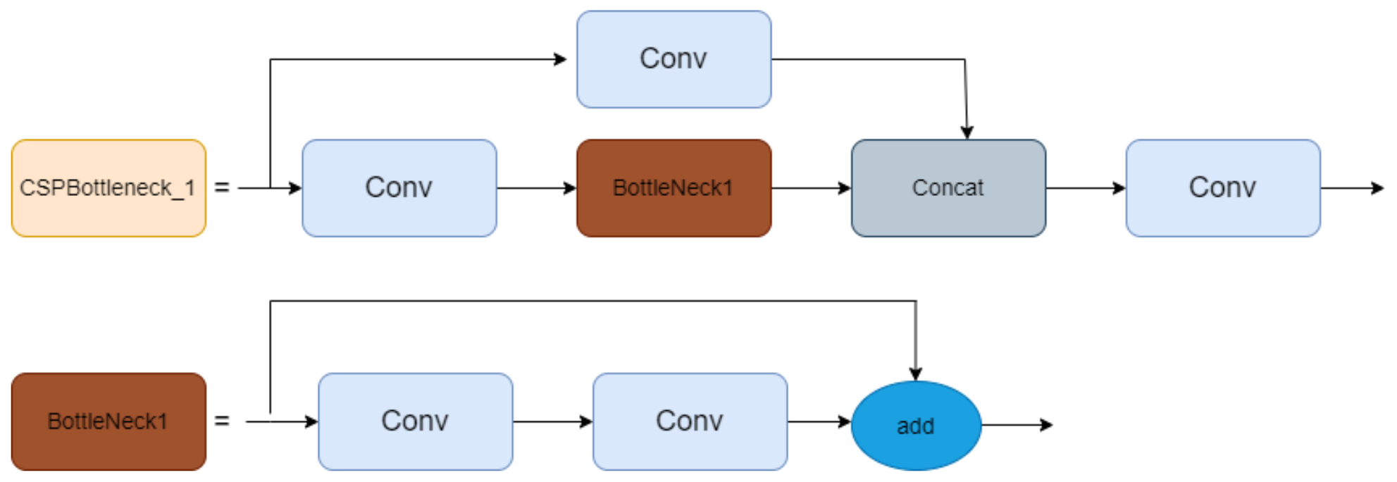
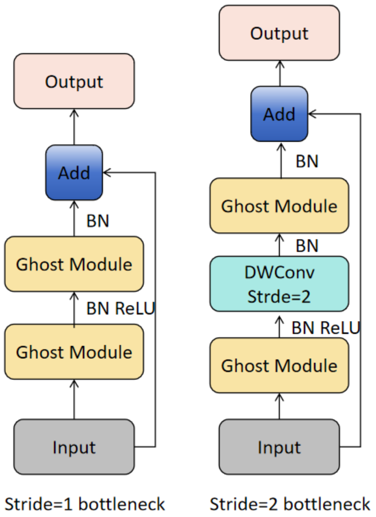
In the backbone network, standard convolutions are replaced with Ghost convolutions, and Bottleneck1 is replaced with GhostBottleneck. This helps reduce the model’s parameter count and computational load, meeting the real-time requirements of underwater operations.
(2)
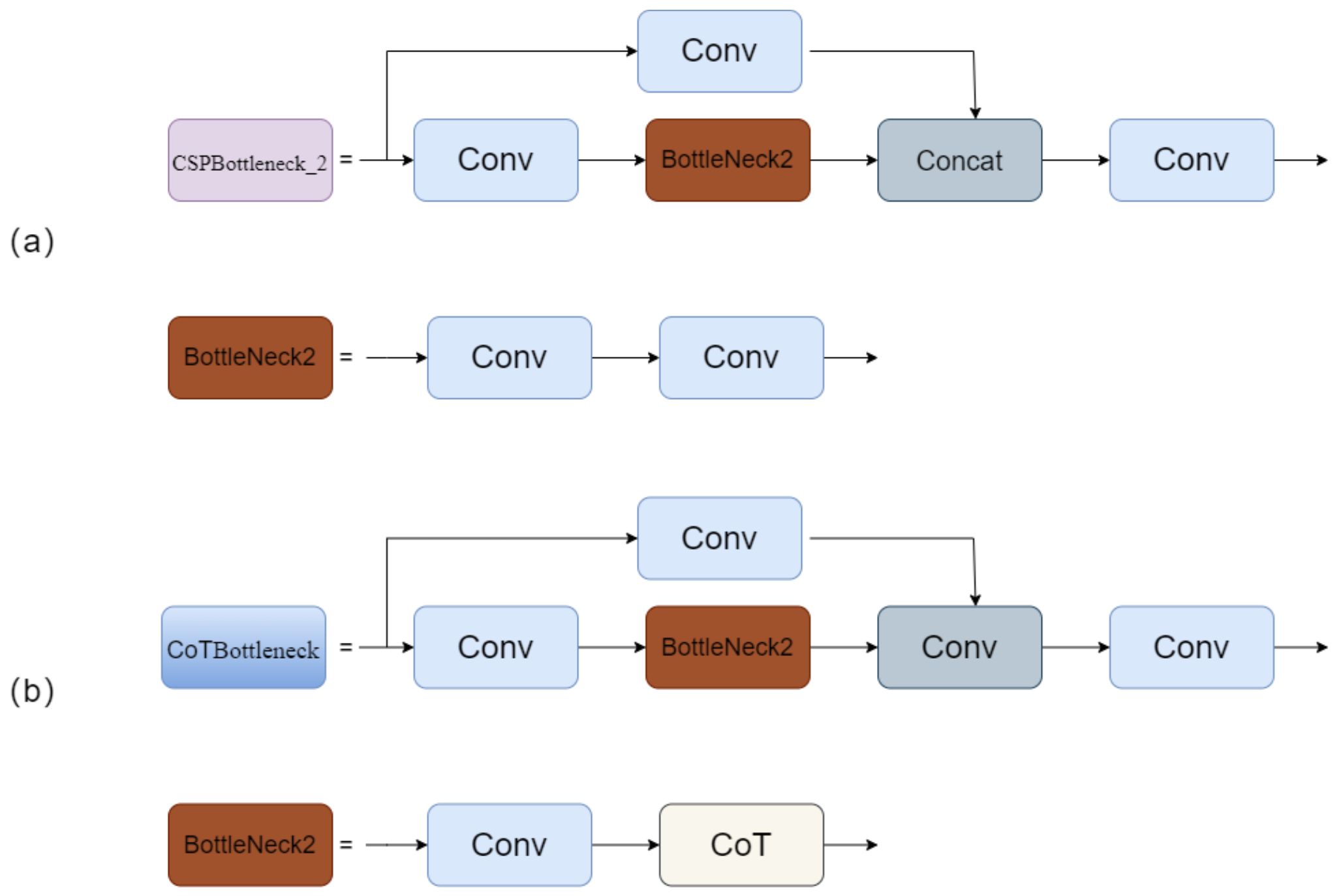
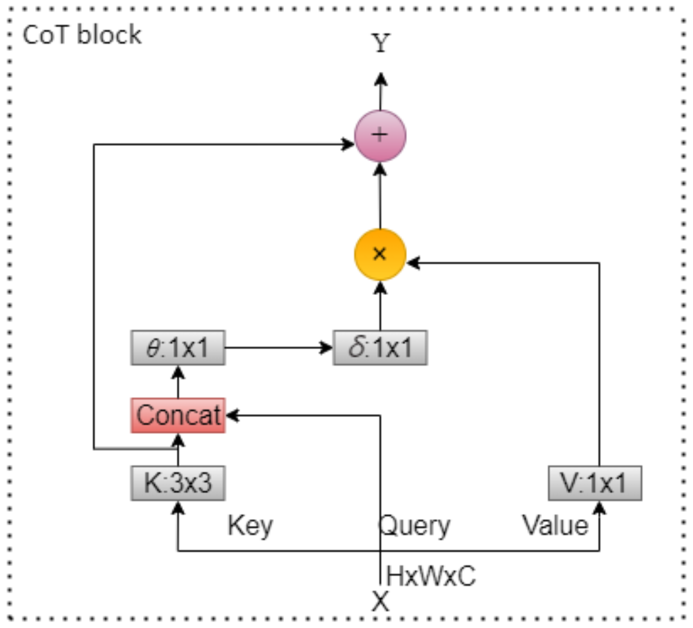
In the feature fusion network, the Contextual Transformer module is introduced into CSPBottleneck_2, replacing the 3 × 3 standard convolution. This utilizes contextual information among input keys to guide self-attention learning, contributing to improved detection accuracy.
(3)
Focal_EIoU Loss (Focal and Efficient Intersection over Union) is employed instead of IoU (Intersection over Union) Loss to enhance the precision of the predicted bounding boxes and accelerate model convergence.
These improvements aim to make the model more adaptable to the poor image quality that is characteristic of underwater environments and, through a lightweight design, cater to the practical application needs of underwater mobile devices.

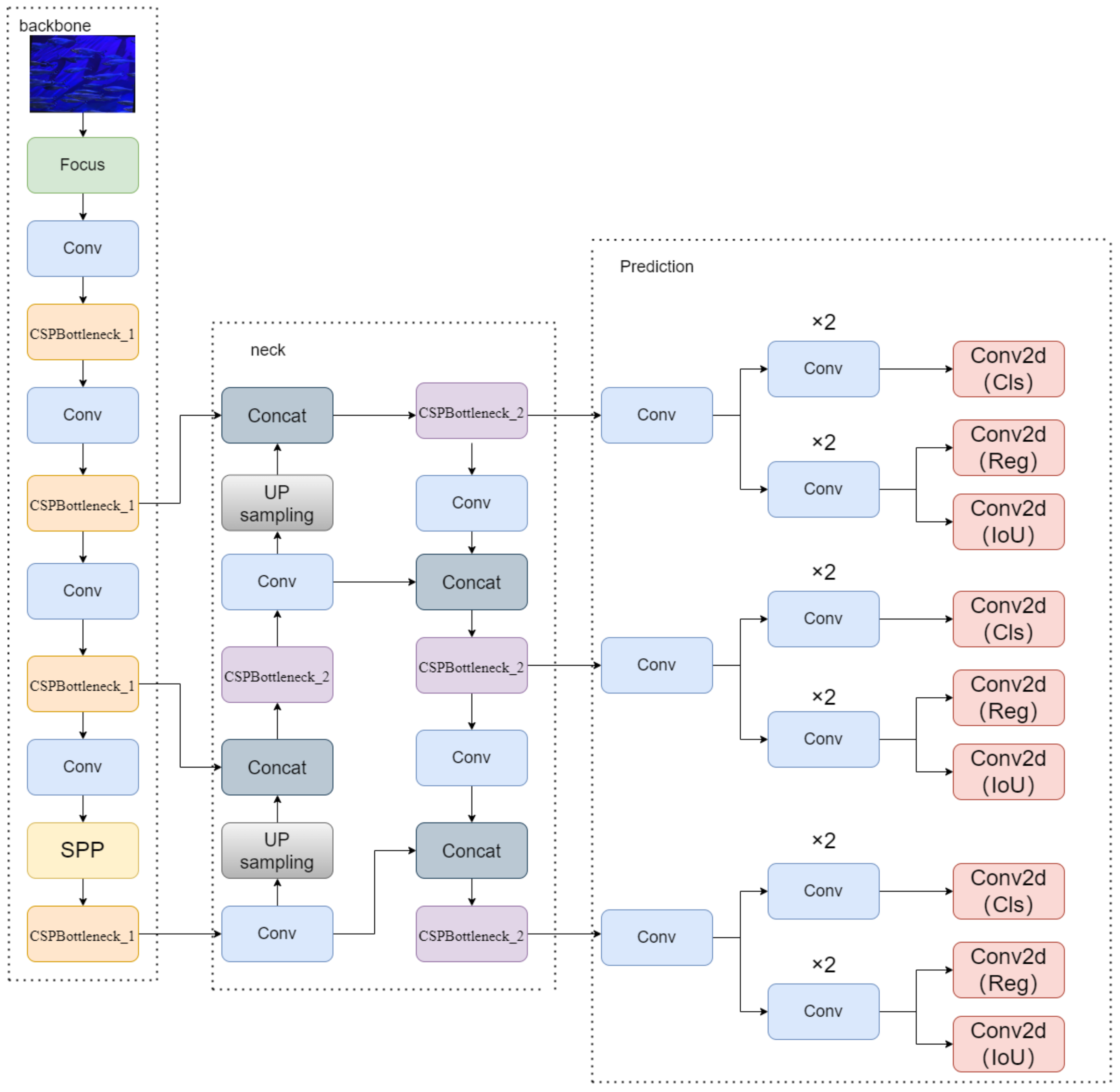
2. YOLOX Network Architecture

YOLOX is a single-stage object detection algorithm, proposed in 2021 by Zheng Ge et al. [25]. It is built upon YOLOv5 and consists mainly of an input end, backbone network, neck network, and Prediction detection layer, as illustrated in Figure 1.
Input End: At the input end of the network, YOLOX adopts the Mosaic data augmentation method. This method involves randomly scaling, cropping, and arranging four training images for mixed splicing. The four images are merged into a new image, which is then fed into the neural network model for training. Each of the images involved in the splicing process has annotated bounding boxes. This approach effectively utilizes information from the training set, allowing the model to better understand and recognize various objects and scenes. An illustrative diagram of the splicing effect is shown in Figure 2.
Backbone Network: The backbone network serves as the main network and adopts the network structure of Darknet53 [26]. Darknet53 is a network structure with 53 convolutional layers. By stacking multiple convolutional and pooling layers, it gradually transforms the input image into feature maps of different scales. These feature maps can contain more semantic information, such as object shapes, textures, and colors.
Neck Network: The neck network functions as the feature fusion network, utilizing the FPN (Feature Pyramid Network) + PAN (Path Aggregation Network) structure for multi-scale feature fusion. The FPN is a top-down structure [27], merging high-level feature maps with upsampled low-level feature maps to create new feature maps conveying strong semantic features. PAN is a bottom-up structure [28], conveying localization information from the bottom layers through downsampling and enabling top-level feature maps to include positional information.
Prediction Detection Layer: The Prediction detection layer performs multi-scale object detection on the feature maps that are extracted by the neck network. By using detection heads of different sizes, it achieves accurate predictions for the image, generating bounding box coordinates and predicting categories.
Compared to YOLOv5, YOLOX introduces innovations such as the decoupled detection head, Anchor-Free, and SimOTA. In YOLOv5, the detection head predicts both classification and localization tasks simultaneously using a 1 × 1 convolution. In contrast, YOLOX employs a decoupled detection head. Initially, it uses a 1 × 1 convolution for dimension reduction, followed by two separate branches, each using a 3 × 3 convolution. This structure not only enhances the detection performance but also accelerates the convergence speed. The Anchor-Free algorithm eliminates the need for anchor points and directly predicts the bounding box position and size for object detection. This approach adapts better to the diversity and variability of objects while reducing the computational complexity. SimOTA is a target tracking algorithm that improves the tracking accuracy and robustness by matching positive samples of the target with surrounding negative samples.

3. Methods

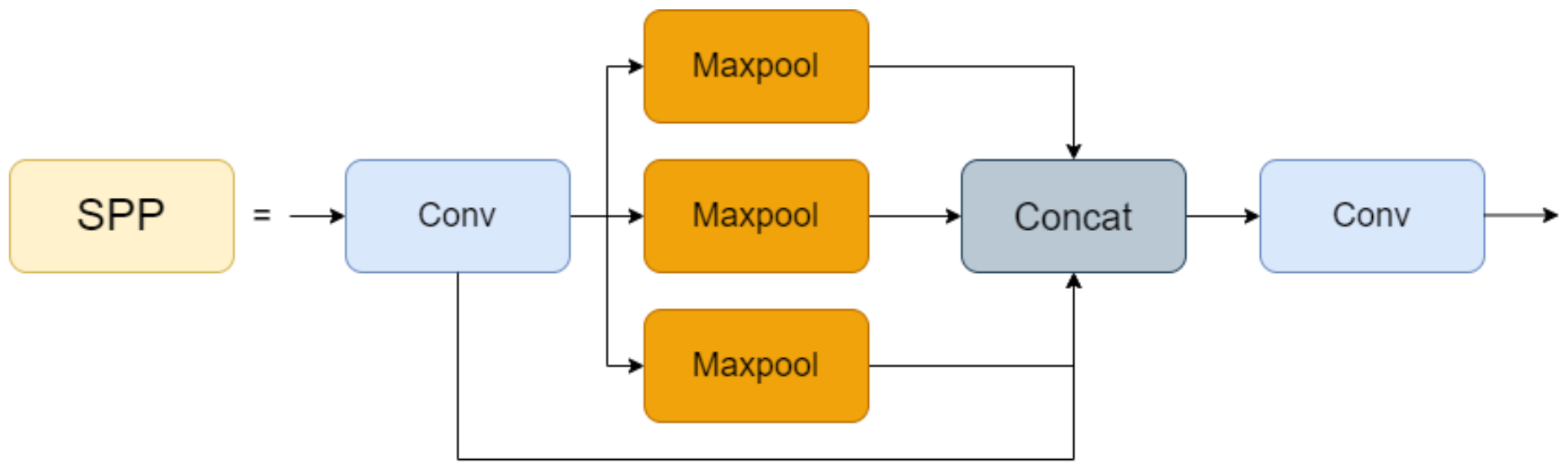
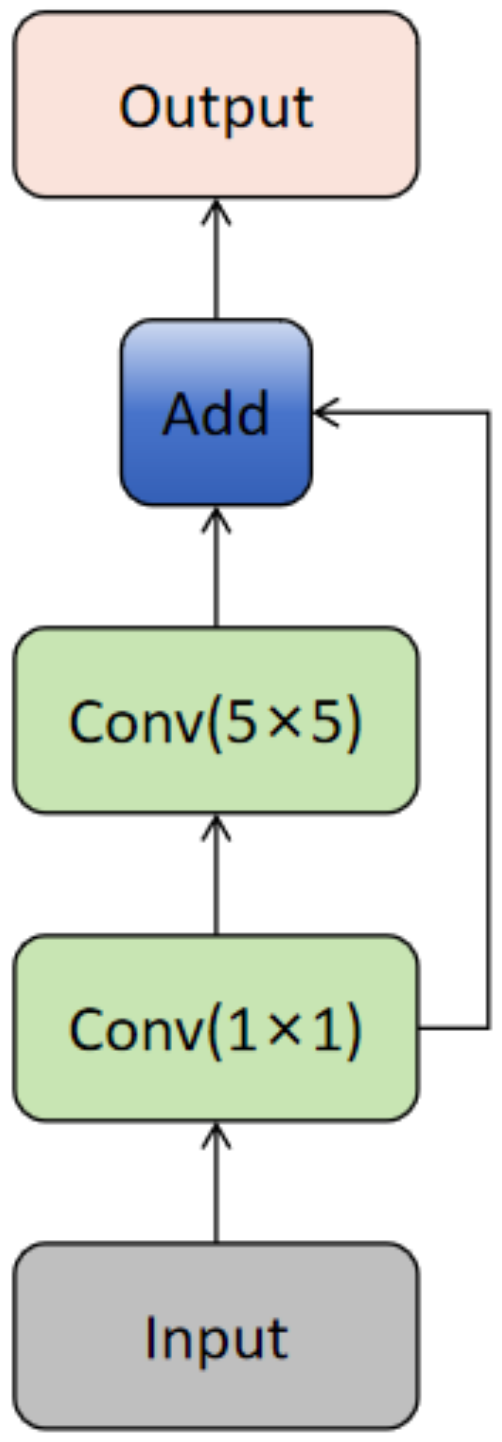
3.1. Improvement Strategies for the Backbone Network

The backbone network of YOLOX consists of CSPDarknet53 and SPP (Spatial Pyramid Pooling) [29] networks. The design of the entire backbone network aims to organically combine these components to capture features at different scales and levels comprehensively. This enhances the accuracy and robustness of the object detection. The architecture is shown in Table 1.
Firstly, the image undergoes processing through the Focus network, which segments the image into sub-feature maps of different sizes. This helps capture detailed information about the target at various scales. Subsequently, each sub-feature map undergoes a series of operations, including three sets of Conv layers and the CSPBottleneck_1 layer. The role of the Conv layers is to extract features from the image, reducing the size of the feature map by half and doubling the number of channels, thereby enhancing the network’s perception of the target. The CSPBottleneck_1 layer divides the feature map into two branches, as illustrated in Figure 3. One branch undergoes channel dimension transformation through a 1 × 1 Conv layer, then passes through a bottleneck1 with a residual structure, and finally concatenates with the other branch, processed through a 1 × 1 Conv layer. The concatenated features then undergo further processing through a 1 × 1 Conv layer. Lastly, the feature map undergoes processing through Conv layers, the SPP network, and the CSPBottleneck_1 layer. The SPP network consists of four branches, as shown in Figure 4. The first branch serves as the direct output, while the remaining three branches perform pooling operations on the feature map using differently sized pooling layers (5 × 5, 9 × 9, 13 × 13). The outputs of these branches are ultimately merged to achieve multi-scale feature fusion, thereby enhancing the model’s detection capability for targets.
In order to reduce the model’s parameter count and computational load, this paper introduces GhostConv (Ghost Convolution) and GhostBottleneck into the backbone network [30], replacing the standard convolutions in the YOLOX network and the Bottleneck1 structure in CSPBottleneck_1. The architecture is shown in Table 2.
Due to the redundancy and similarity of features that are often present in feature maps generated by standard convolutions, Han et al. proposed an innovative structure called the Ghost Module to address this issue. The Ghost Module significantly reduces the model’s complexity without reducing the number of feature maps. The schematic diagram of this structure is shown in Figure 5. Firstly, intrinsic feature maps are extracted using a 1 × 1 convolution layer. Then, more economical linear operations are applied to generate the remaining feature maps using a 5 × 5 convolution layer. Finally, the outputs of these two layers are concatenated to form the final feature map of the Ghost Module.
The Ghost Bottleneck is divided into two structures based on the stride, as shown in Figure 6. The Bottleneck with a stride of 1 consists of two concatenated Ghost Modules. The first Ghost Module is used to expand the number of channels, and the second Ghost Module reduces the number of channels to match the input channel count. This structure is employed to increase the network’s depth without compressing the height and width of the input feature layer. The Bottleneck with a stride of 2 introduces a Deepwise convolution with a stride of 2 between the two Ghost Modules, compressing the height and width of the input feature layer and altering its shape. Since the CSPBottleneck_1 in the YOLOX model uses a convolution with a stride of 1, the Ghost Bottleneck in this paper adopts a structure with a stride of 1.

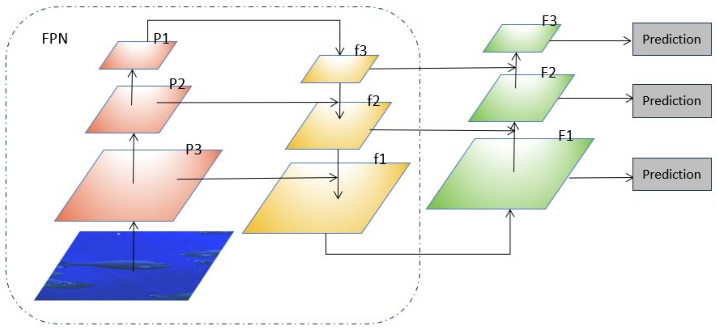
3.2. Feature Fusion Network Improvement Strategy

The neck network of YOLOX adopts the PAFPN structure for fusion, as shown in Figure 7. The original image undergoes feature extraction by the backbone network, producing three feature layers of different sizes: P1, P2, and P3. In the FPN structure, P1, P2, and P3 are fused through lateral connections and top-down sampling paths to generate the fused feature maps f1, f2, and f3. This structure merges high-level and low-level feature maps, facilitating the transmission of strong semantic features. Then, f1, f2, and f3 are further fused through lateral connections and bottom-up sampling to generate the feature maps F1, F2, and F3, enabling the transmission of positional information from the bottom layers to the top layers. Finally, the fused feature maps are input into the prediction layer to achieve accurate image prediction. In this paper, the CoT block is introduced into CSPBottleneck_2 to utilize context information between input keys to guide self-attention learning, as depicted in Figure 8.
The Transformer structure based on self-attention possesses powerful global modeling capabilities and has achieved remarkable success in natural language processing. In recent years, it has also demonstrated good performance in computer vision tasks. However, most Transformer structures directly apply self-attention on two-dimensional feature maps to obtain attention matrices based on a query and key for each spatial position. However, the contextual information between adjacent keys is not fully utilized. To address the problem of feature loss in Transformer, Li et al. proposed a new attention structure [31], namely, the Contextual Transformer (CoT) block. This module promotes self-attention learning by leveraging contextual information between keys, ultimately enhancing the network’s representational capacity.
The CoT block employs a Transformer structure to simplify the extraction process of effectively related features over long distances in the image, expanding the receptive field and better utilizing the context features of key points. Firstly, query vectors Q (Query), key vectors K (Keys), and value vectors V (Values) are created using a weight matrix. Then, by applying a 3 × 3 convolution operation to adjacent keys, the contextualization of key feature information is performed, transforming it into a representation of static feature information. The contextualized key features are then concatenated with the query vector and undergo two consecutive 1 × 1 convolutions to generate an attention matrix. This concatenation process connects the query vector with the contextualized key features of all key vectors, enabling the attention matrix to learn and generate under the guidance of static contextual information, effectively enhancing self-attention. Subsequently, by multiplying the attention matrix with the value vector, dynamic feature information of the input value vector is obtained. Finally, the static feature information and dynamic feature information are added together as the output. The structure diagram of the CoT block is shown in Figure 9.
From a computational perspective, for the input feature X , first, define three variables K , Q , and V , representing the query vector Q , key vector K , and value vector V , respectively. Context encoding of the input keys is performed through a 3 × 3 convolution to obtain the static contextual features K 1 between locally adjacent keys. K 1 is then concatenated with Q , and through two consecutive 1 × 1 convolutions, a matrix, A , is obtained. The expression for matrix A is shown in Equation (1):
A = [ K 1 , Q ] W θ W δ
Then, multiplying matrix A by V obtains the dynamic contextual features K 2 . The expression for K 2 is shown in Equation (2):
K 2 = V A
Finally, the local static contextual feature information K 1 and dynamic contextual feature information K 2 are added together to obtain the output Y . The expression for Y is shown in Equation (3):
Y = K 1 + K 2
By introducing the CoT block into the feature fusion network, it helps to increase the receptive field. Combining contextual information and self-attention learning enhances the network’s ability to integrate local and global information in images. Since the CoT block focuses on long-distance correlations, it can better handle the relationships between objects, contributing to improved robustness and generalization in object detection.

3.3. Loss Function Improvement

The localization loss function, also known as the regression loss function, aims to measure the distance deviation between the final predicted box and the ground truth box. This distance difference is calculated through a specific function, transforming it into a loss value. Subsequently, the weight parameters are adjusted through backpropagation of errors to gradually bring the predicted box closer to the ground truth box. The original YOLOX algorithm uses IoU Loss as the localization loss function. IoU is a simple metric for measuring the distance between the predicted box and the target box by calculating the intersection over union of the predicted box and the ground truth box. When the predicted box and the ground truth box do not intersect, the IoU value is 0, which does not accurately reflect the distance between them. Additionally, IoU cannot precisely indicate the degree of overlap between the predicted box and the ground truth box.
To address the aforementioned issue, this paper replaces IoU Loss with Focal_EIoU Loss [32], as shown in Equation (4). Focal_EIoU Loss effectively tackles the problem of a sample imbalance and enhances the accuracy and robustness of object detection by combining the class recognition capability of Focal Loss and the positional accuracy of EIoU Loss. Specifically, Focal_EIoU Loss focuses on difficult and misclassified samples by reducing the weight of easily classifiable samples. Here, γ is an adjustment factor controlling the curvature of the curve, so that the loss for correctly classified samples is reduced, while the loss for misclassified samples is increased. EIoU Loss consists of three parts: IoU loss, center distance loss, and width–height loss, which consider the overlap area of the bounding box regression, the distance between centers, and the differences in width and height of the edges. This formulation helps mitigate the issues that are present in IoU Loss to some extent.
F o c a l _ E I o U   L o s s = I o U γ E I o U L o s s E I o U L o s s = L o s s I o U + L o s s d i s + L o s s a s p   = 1 I o U + p 2 ( b , b g t ) c 2 + p 2 ( w , w g t ) C w 2 + p 2 ( h , h g t ) C h 2

4. Experiments

4.1. Experimental Environment and Settings

All experiments in this article were conducted in the same environment, with detailed configurations as shown in Table 3.
The experiment employed the single-stage object detection algorithm YOLOXs. The detailed experimental parameters are provided in Table 4.

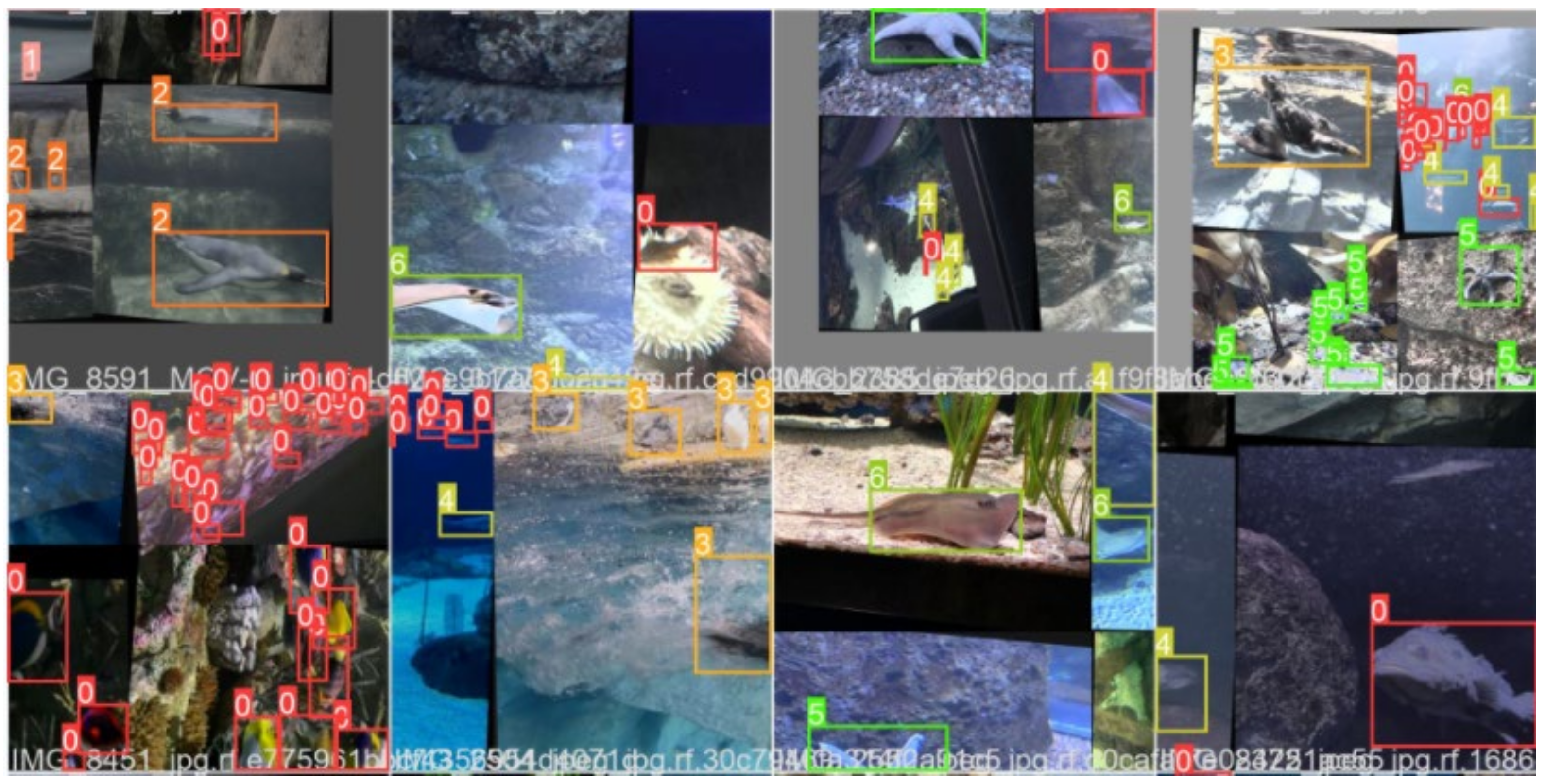
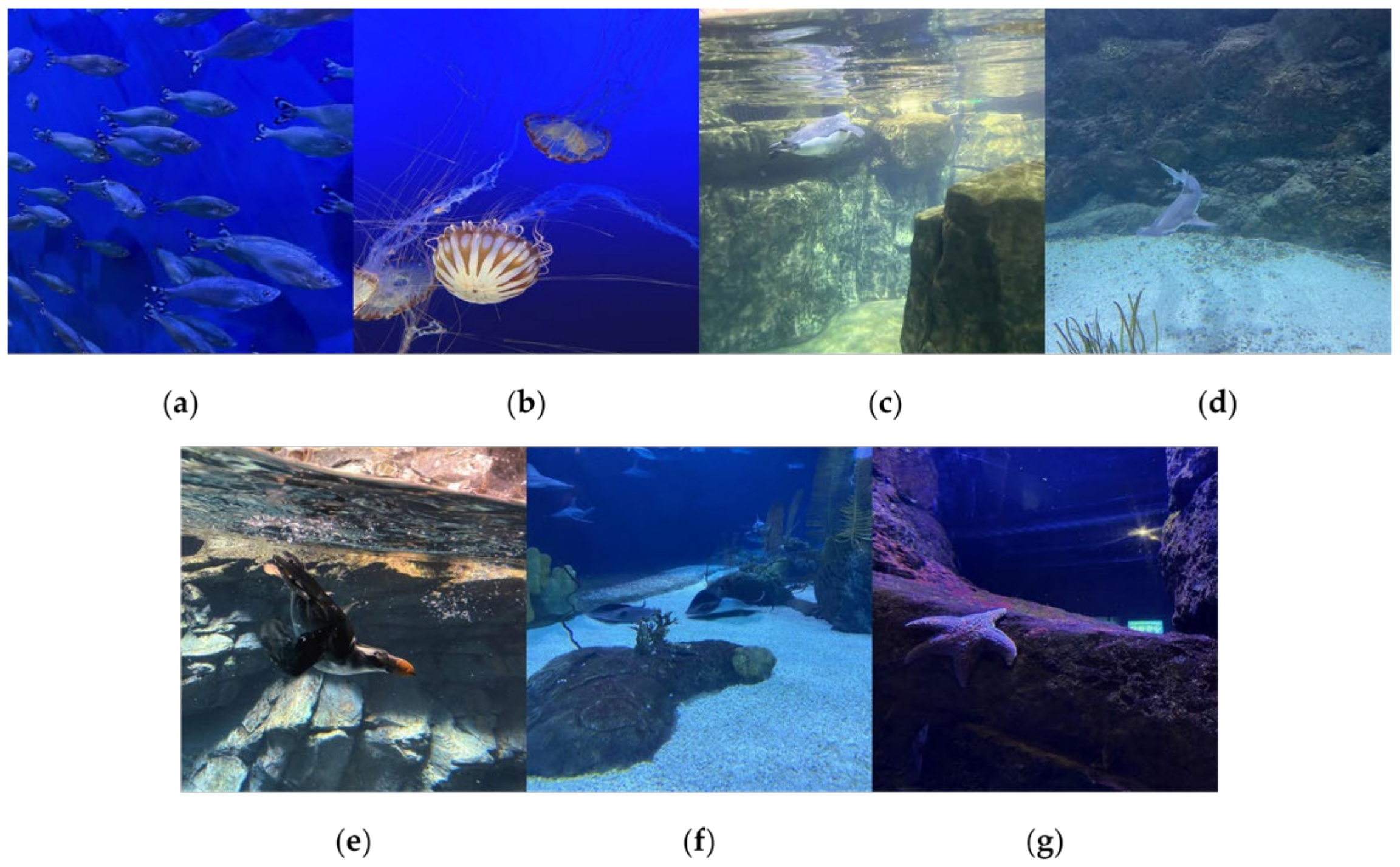
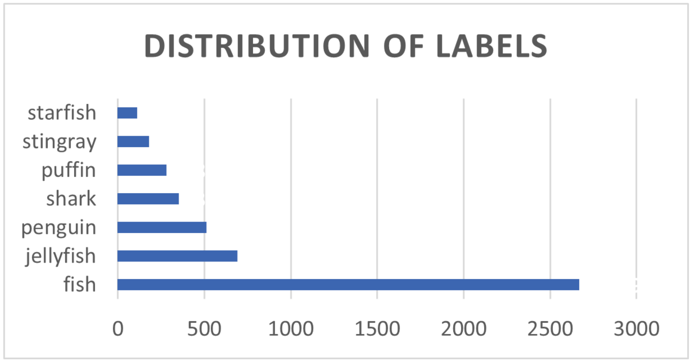
4.2. Introduction to the Experimental Dataset

The dataset used in this paper comprises 638 images collected by Roboflow from two aquariums in the United States: the Henry Doorly Zoo in Omaha and the National Aquarium in Baltimore [33]. The Roboflow team annotated the images for object detection. This dataset includes seven marine creatures, as shown in Figure 10, namely, fish, jellyfish, penguins, sharks, parrotfish, yellow tangs, and starfish. Through techniques such as rotation and flipping for data augmentation, the dataset was expanded to 4670 images. The distribution of each category in the dataset is depicted in Figure 11.

4.3. Implementation Details

To provide a more intuitive and accurate evaluation of object detection algorithms and facilitate comparisons between different object detection algorithms, this paper employs several commonly used evaluation metrics for object detection networks. These metrics include precision, recall, AP (average precision), mAP (mean average precision), parameters, GFLOPs (Giga Floating-point Operations per Second), FPS (Frames Per Second), and model size.
Precision, representing accuracy, evaluates the model’s correctness by calculating the ratio of true positive samples (correctly predicted positive samples) to the total samples that are predicted as positive by the model. T P denotes the number of actual positive samples that are predicted as positive by the model, and F P represents the number of actual negative samples that are predicted as positive by the model. The calculation formula is as shown in Equation (5).
P r e c i s i o n = T P T P + F P
Recall, also known as sensitivity or the true positive rate, refers to the proportion of correctly predicted positive samples among all actual positive samples. F N represents the number of actual positive samples that are predicted as negative by the model. The calculation formula is as shown in Equation (6).
R e c a l l = T P T P + F N
A P , or average precision, is a metric used to evaluate the accuracy of a model in multi-class classification problems, with values ranging from 0 to 1. It is obtained by calculating the average precision and recall at different confidence thresholds. One common method for calculating A P is by plotting the precision–recall (PR) curve, where the x-axis represents recall and the y-axis represents precision. A larger area under the PR curve indicates a better model performance, as it signifies the model’s ability to maintain high precision and recall at different thresholds. The calculation formula is as shown in Equation (7).
A P = 0 1 P ( R ) d r
m A P , or mean average precision, is the average value of A P across different classes. It is calculated as the mean of A P for each class, as shown in Equation (8), where ‘m’ represents the number of classes or labels.
m A P = 1 m i = 1 m A P i
The size of m A P depends on the predefined I o U threshold, where I o U (intersection over union) is a metric that is used to measure the overlap between the predicted boxes and ground truth boxes. It is calculated by determining the ratio of the intersection area of the predicted box and the ground truth box to the union area of the two. The specific formula is shown in Equation (9):
I o U = A B A B
where A represents the predicted box, and B represents the ground truth box. A B denotes the intersection area between the predicted box and the ground truth box, and A B represents the union area of the predicted box and the ground truth box.
In object detection, besides the commonly mentioned evaluation parameters, there are other metrics that can also assess a model’s performance. Parameters refer to the total number of parameters in the model that need to be learned, including weights and biases. The parameter count is typically used to measure the size of the model, indicating the amount of the storage space that the model occupies. In object detection, a smaller model parameter count is beneficial for deployment on resource-constrained devices, such as mobile devices or embedded systems. GFLOPs indicate the number of floating-point operations that the model performs per second and is commonly used to measure the computational complexity of the model. GFLOPs depend on the model’s architecture, the number of layers, and the resolution of input images. Lower GFLOPs suggest that the model has a relatively lower computational overhead during inference, making it more suitable for environments with limited computational resources. FPS represents the number of frames processed per second in an image sequence, serving as a metric for measuring the inference speed of the model. In real-time applications, a higher FPS indicates that the model can process input images more quickly, which is crucial for scenarios requiring a real-time response, such as video surveillance and autonomous driving. Therefore, when selecting object detection models, it is essential to consider multiple aspects, including accuracy, computational complexity, and inference speed. The choice should be made based on the specific requirements of the application. In underwater object detection applications, where the memory in underwater devices is limited, researchers need to design smaller and more efficient model structures and parameter settings to reduce computational and storage requirements without sacrificing performance.

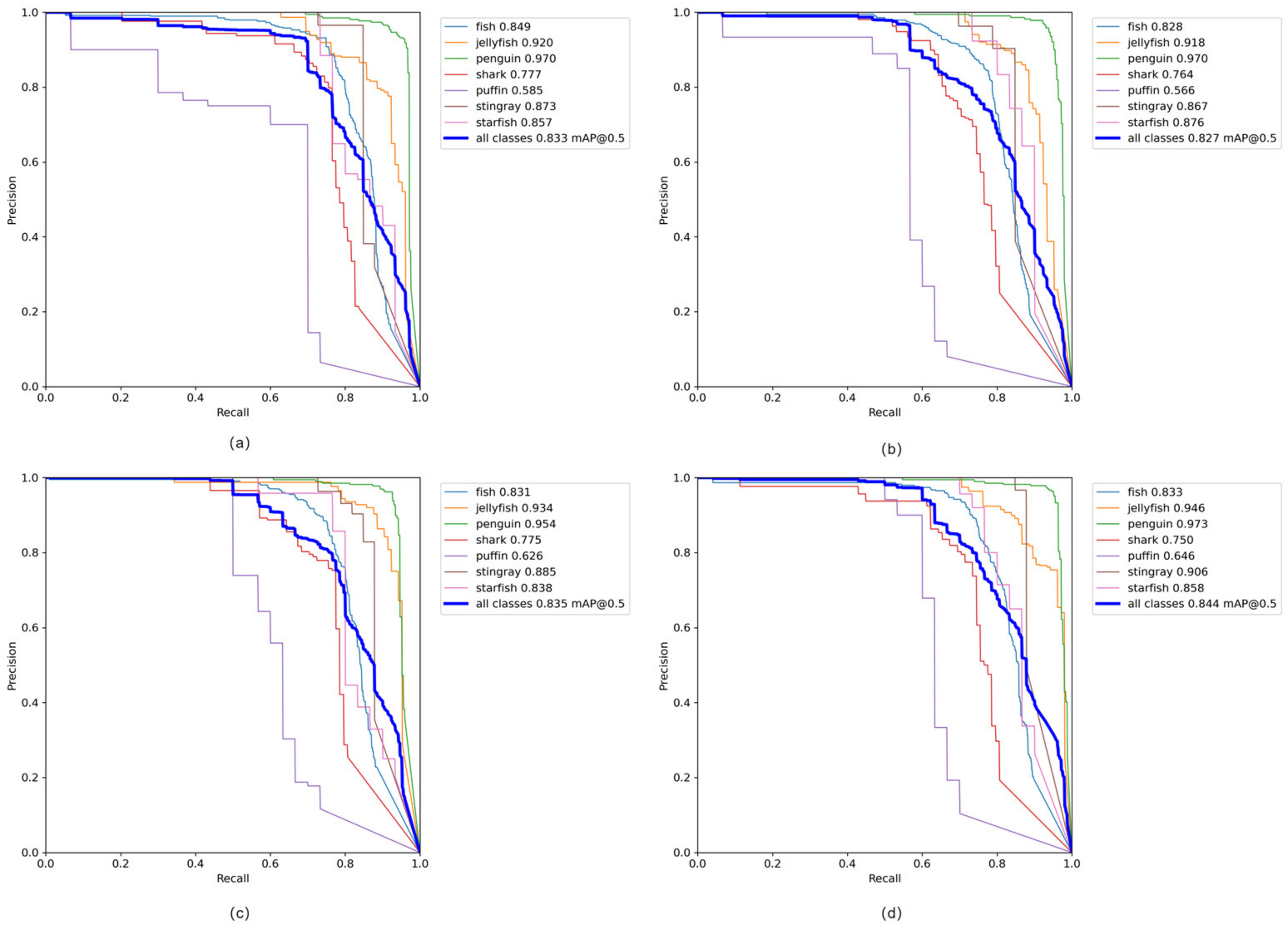
4.4. Ablation Experiments

In order to validate the effectiveness of each improvement module, detailed ablation experiments were conducted in this study. Experiment 1 involved the YOLOXs network; Experiment 2 introduced Ghost Conv and Ghost Bottleneck into the backbone network based on Experiment 1; Experiment 3 introduced a CoT block into the feature fusion network based on Experiment 2; Experiment 4 represented the final improved network, replacing the IoU Loss function with Focal_EIoU Loss based on Experiment 3. Table 5 shows the impact of different improvement strategies on the model’s detection performance, while Table 6 demonstrates the influence of different improvement strategies on the model’s complexity.
Based on the comprehensive analysis of the results, it is evident that with the introduction of Ghost Conv and Ghost Bottleneck into the backbone network, although the mAP value decreased by 0.6%, there were significant reductions in parameters, computations, and model size. Specifically, the parameter count decreased by 1.99M, representing a reduction of approximately 24.47%, while the computation decreased by 5.7, with a reduction of approximately 26.39%. Moreover, the model size decreased by 3.7, indicating a reduction of around 23.87%. This suggests that such a strategy effectively addresses the limited memory capacity and computational resources of small underwater devices, meeting the requirements of practical applications.
Upon introducing the CoT block into the feature fusion network, the mAP value increased by 0.8%. This indicates that this strategy, by incorporating contextual information, assists the model in better understanding the position and semantic information of target objects in the entire image, thereby improving the accuracy of the target localization. However, there was a significant decrease in FPS, possibly due to the Contextual Transformer module needing to capture long-range dependencies in the input data, leading to increased computation steps and time, resulting in the decrease in FPS. Upon replacing the IoU Loss function with Focal_EIoU Loss, the mAP value increased by 0.9%. This suggests that Focal_EIoU Loss, by introducing a more accurate measure of target localization, can better optimize the object detection model and improve the detection performance.
In summary, compared to the initial model, the improved YOLOXs model achieved a 1.1% increase in mAP value, a reduction of 2.01M parameters, a decrease of 5.7 GFLOPs, and a reduction in model size of 3.7 MB.
According to the experimental results, four sets of PR (precision–recall) curve graphs were plotted, as shown in Figure 12. The four graphs, respectively, display the PR curves for each class and the average PR curve for all classes. It can be observed that the area enclosed by the PR curve of the improved YOLOX is larger than that of the other four methods. This indicates that the four proposed improvement methods in this paper can enhance the model’s performance to some extent, validating the effectiveness of these improvement methods.

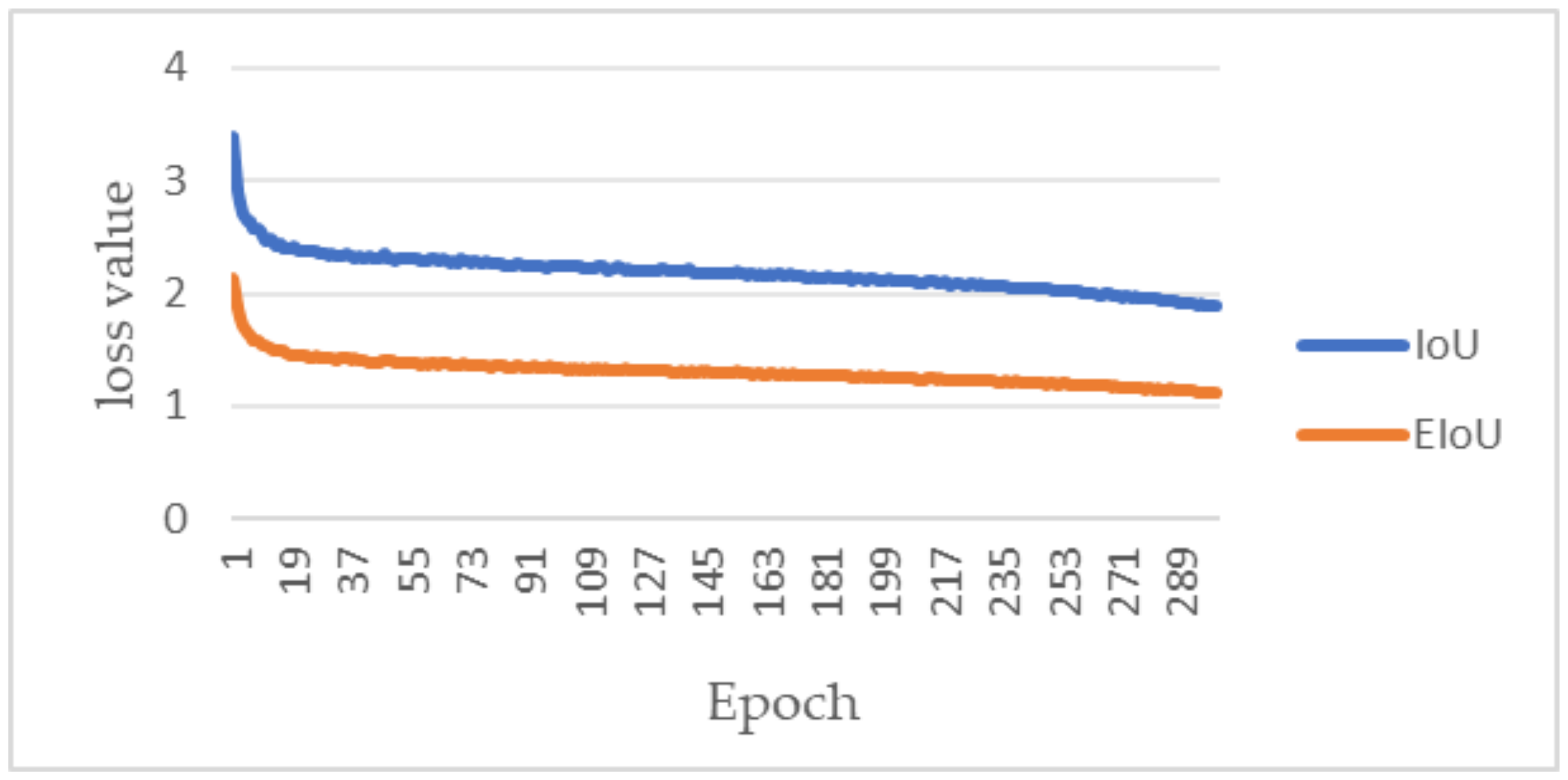
4.5. Comparative Performance Analysis of Different Loss Functions

In the model improvement, YOLOXs replaced IoU Loss with Focal_EIoU Loss as the localization loss function. Figure 12 shows the variation in loss values for the two loss functions under the same experimental environment. From Figure 13, it can be observed that adopting Focal_EIoU Loss results in faster and smoother model convergence, and it has the lowest loss values.

4.6. Cross-Sectional Comparative Analysis of Different Detection Models

To further demonstrate that the improved model in this paper performs better for underwater object detection compared to other models, YOLOXs before and after improvement is trained and compared with other classical models using the same training parameters and dataset. The results are shown in Table 7. From the comparison, it can be observed that, relative to current mainstream detection models such as Faster-RCNN, Cascade R-CNN, SSD, YOLOv3, YOLOv5s, and yolov7_tiny [34], the model proposed in this paper achieves the highest mAP value of 84.4% for the underwater organism dataset. In terms of parameter count and computational complexity, the model in this paper is significantly superior to other models. Overall, the algorithm in this paper shows good performance in these metrics, confirming the advantages of the proposed improvement methods.

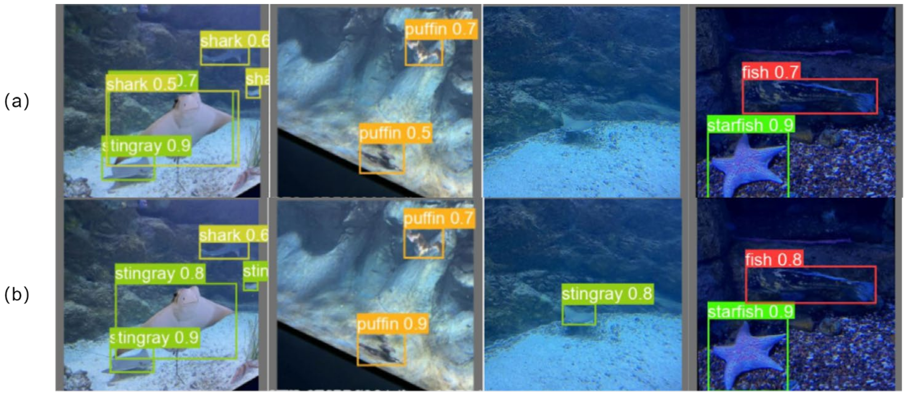
4.7. Detection Performance Comparison and Analysis

To visually showcase the performance of the improved model, this study selected images from the validation set to compare and display the detection results before and after improvement. As shown in Figure 14, the top row (a) displays the detection results of the original YOLOXs model, while the bottom row (b) shows the detection results of the improved YOLOXs model. Through these images, it is evident that the original YOLOXs model in the top row exhibits issues of missed detections and false positives in underwater images with blurriness, and it has lower accuracy in detecting small objects. In contrast, the improved model in the bottom row demonstrates higher accuracy. In summary, the proposed model shows excellent detection capabilities in complex environments.

5. Conclusions

Underwater target detection serves as the foundation for underwater robots to achieve automated detection and grasping operations. To facilitate the development and utilization of marine resources, focusing on marine organisms as the detection target, this paper proposes a novel model named YOLOXs-GCE, which is an improvement compared with YOLOXs. Firstly, Ghost Conv and Ghost Bottleneck are introduced into the backbone network, significantly reducing the model’s parameter count, computational load, and size, while sacrificing a minimal amount of model accuracy. This lightweight processing method effectively addresses the challenge of underwater image processing under resource-constrained conditions. Subsequently, the CoT block is incorporated into the feature fusion network, enhancing the model’s understanding, representation, and generalization capabilities through advantages such as context awareness, parameter sharing, and parallel computing. Finally, IoU Loss is replaced with Focal_EIoU Loss to mitigate the issue of imbalanced positive and negative samples, thereby improving the model’s localization ability, prediction performance, and convergence speed. Our experimental results demonstrate that the improved YOLOXs-GCE model achieves an mAP value of 84.4% on the underwater biological dataset detection, with 6.06M parameters, a computational load of 15.9, and a model size of 11.8M.
This study confirms that YOLOXs-GCE, with its lightweight design and efficient performance, is particularly suitable for underwater equipment with limited resources. It demonstrates outstanding robustness in addressing the variability and challenges of the underwater environment. Looking ahead, we plan to further validate the effectiveness of the YOLOXs-GCE model on a wider range of underwater image datasets and explore the model’s application potential in actual underwater environments, such as the autonomous navigation of underwater devices and biodiversity monitoring. Additionally, considering the real-time requirements and resource limitations that may be encountered in practical applications, we will continue to optimize the detection accuracy of the model while reducing its complexity. Although this study has achieved certain results, further improvement in detection accuracy remains a focus of our research. We look forward to pushing the YOLOXs-GCE model into a broader range of underwater application scenarios through continuous efforts.

Author Contributions

Conceptualization, H.W. and P.Z.; methodology, P.Z.; software, M.Y.; validation, P.Z.; formal analysis, X.Y.; investigation, M.Y.; resources, H.W.; data curation, X.Y.; writing—original draft preparation, P.Z.; writing—review and editing, H.W.; funding acquisition, H.W. All authors have read and agreed to the published version of the manuscript.

Funding

This research was supported by a key project funded by the Hubei Provincial Department of Education, China, under grant number D20201601.

Institutional Review Board Statement

Not applicable.

Informed Consent Statement

Not applicable.

Data Availability Statement

The data are available online at Aquarium Combined Dataset > Overview (www.roboflow.com, accessed on 1 July 2023).

Conflicts of Interest

The authors declare no conflicts of interest.

References

  1. Yang, Y.Y. A Preliminary Exploration of the Current Status of China’s Marine Resources in the Perspective of Sustainable Development. Land Nat. Resour. Res. 2020, 2020, 37–38. [Google Scholar]
  2. Dalal, N.; Triggs, B. Histograms of oriented gradients for human detection. In Proceedings of the 2005 IEEE Computer Society Conference on Computer Vision and Pattern Recognition (CVPR’05), San Diego, CA, USA, 20–26 June 2005; Volume 1, pp. 886–893. [Google Scholar]
  3. Chen, P.H.; Lin, C.J.; Schölkopf, B. A tutorial on v-support vector machines. Appl. Stoch. Models Bus. Ind. 2005, 21, 111–136. [Google Scholar] [CrossRef]
  4. Simonyan, K.; Zisserman, A. Very deep convolutional networks for large-scale image recognition. arXiv 2014, arXiv:1409.1556. [Google Scholar]
  5. Szegedy, C.; Liu, W.; Jia, Y.; Sermanet, P.; Reed, S.; Anguelov, D.; Erhan, D.; Vanhoucke, V.; Rabinovich, A. Going deeper with convolutions. In Proceedings of the IEEE Conference on Computer Vision and Pattern Recognition, Boston, MA, USA, 7–12 June 2015; pp. 1–9. [Google Scholar]
  6. Girshick, R.; Donahue, J.; Darrell, T.; Malik, J. Rich feature hierarchies for accurate object detection and semantic segmentation. In Proceedings of the IEEE Conference on Computer Vision and Pattern Recognition, Columbus, OH, USA, 23–28 June 2014; pp. 580–587. [Google Scholar]
  7. Clevert, D.A.; Unterthiner, T.; Hochreiter, S. Fast and accurate deep network learning by exponential linear units (elus). arXiv 2015, arXiv:1511.07289. [Google Scholar]
  8. Ren, S.; He, K.; Girshick, R.; Sun, J. Faster r-cnn: Towards real-time object detection with region proposal networks. In Advances in Neural Information Processing Systems; MIT Press: Cambridge, MA, USA, 2015; Volume 28. [Google Scholar]
  9. Cai, Z.; Vasconcelos, N. Cascade r-cnn: Delving into high quality object detection. In Proceedings of the IEEE Conference on Computer Vision and Pattern Recognition, Salt Lake City, UT, USA, 18–23 June 2018; pp. 6154–6162. [Google Scholar]
  10. Liu, W.; Anguelov, D.; Erhan, D. Ssd: Single shot multibox detector. In Proceedings of the Computer Vision—ECCV 2016: 14th European Conference, Amsterdam, The Netherlands, 11–14 October 2016; Proceedings, Part I 14. Springer International Publishing: Berlin/Heidelberg, Germany, 2016; pp. 21–37. [Google Scholar]
  11. Redmon, J.; Divvala, S.; Girshick, R.; Farhadi, A. You only look once: Unified, real-time object detection. In Proceedings of the IEEE Conference on Computer Vision and Pattern Recognition, Las Vegas, NV, USA, 27–30 June 2016; pp. 779–788. [Google Scholar]
  12. Redmon, J.; Farhadi, A. YOLO9000: Better, faster, stronger. In Proceedings of the IEEE Conference on Computer Vision and Pattern Recognition, Honolulu, HI, USA, 21–26 July 2017; pp. 7263–7271. [Google Scholar]
  13. Redmon, J.; Farhadi, A. Yolov3: An incremental improvement. arXiv 2018, arXiv:1804.02767. [Google Scholar]
  14. Bochkovskiy, A.; Wang, C.Y.; Liao, H.Y.M. Yolov4: Optimal speed and accuracy of object detection. arXiv 2020, arXiv:2004.10934. [Google Scholar]
  15. Zhu, X.; Lyu, S.; Wang, X.; Zhao, Q. TPH-YOLOv5: Improved YOLOv5 based on transformer prediction head for object detection on drone-captured scenarios. In Proceedings of the IEEE/CVF International Conference on Computer Vision, Montreal, BC, Canada, 11–17 October 2021; pp. 2778–2788. [Google Scholar]
  16. Moniruzzaman, M.; Islam, S.M.S.; Lavery, P.; Bennamoun, M. Faster R-CNN based deep learning for seagrass detection from underwater digital images. In Proceedings of the 2019 Digital Image Computing: Techniques and Applications (DICTA), Perth, Australia, 2–4 December 2019; pp. 1–7. [Google Scholar]
  17. Jalal, A.; Salman, A.; Mian, A.; Shortis, M.; Shafait, F. Fish detection and species classification in underwater environments using deep learning with temporal information. Ecol. Inform. 2020, 57, 101088. [Google Scholar] [CrossRef]
  18. Liu, T.; Xu, C.; Liu, H.Z. Improved Underwater Object Detection Based on YOLOv3. In Proceedings of the 25th Annual Conference on New Technologies and Applications in Networking 2021, organized by the Network Application Branch of the China Computer Users Association, Lijiang, China, 29 October–1 November 2021; pp. 159–162. [Google Scholar]
  19. Huang, T.H.; Gao, X.Y.; Huang, C.D. Research on Underwater Object Detection Algorithm Based on FAttention-YOLOv5. Microelectron. Comput. 2022, 39, 60–68. [Google Scholar]
  20. Huang, M.; Ye, J.; Zhu, S.; Chen, Y.; Wu, Y.; Wu, D.; Feng, S.; Shu, F. An underwater image color correction algorithm based on underwater scene prior and residual network. In Proceedings of the International Conference on Artificial Intelligence and Security, Qinghai, China, 22–26 July 2022; Springer: Berlin/Heidelberg, Germany, 2022; pp. 129–139. [Google Scholar]
  21. Yin, M.; Du, X.; Liu, W.; Yu, L.; Xing, Y. Multiscale fusion algorithm for underwater image enhancement based on color preser-vation. IEEE Sens. J. 2023, 23, 7728–7740. [Google Scholar] [CrossRef]
  22. Tao, Y.; Dong, L.; Xu, L.; Chen, G.; Xu, W. An effective and robust underwater image enhancement method based on color correction and artificial multi-exposure fusion. Multimed. Tools Appl. 2023, 84, 1–21. [Google Scholar] [CrossRef]
  23. Yin, S.; Hu, S.; Wang, Y.; Wang, W.; Li, C.; Yang, Y.-H. Degradation-aware and color-corrected network for underwater image enhancement. Knowl. Based Syst. 2022, 258, 109997. [Google Scholar] [CrossRef]
  24. Xu, S.; Zhang, J.; Bo, L.; Li, H.; Zhang, H.; Zhong, Z.; Yuan, D. In Retinex based underwater image enhancement using attenuation compensated color balance and gamma correction. In Proceedings of the International Symposium on Artificial Intelligence and Robotics 2021, Fukuoka, Japan, 21–27 August 2021; SPIE: Bellingham, WA, USA, 2021; pp. 321–334. [Google Scholar]
  25. Ge, Z.; Liu, S.; Wang, F.; Li, Z.; Sun, J. Yolox: Exceeding yolo series in 2021. arXiv 2021, arXiv:2107.08430. [Google Scholar]
  26. Wang, C.-Y.; Liao, H.-Y.M.; Wu, Y.-H.; Chen, P.-Y.; Hsieh, J.-W.; Yeh, I.-H. In Cspnet: A new backbone that can enhance learning capability of cnn. In Proceedings of the IEEE/CVF Conference on Computer Vision and Pattern Recognition Workshops, Seattle, WA, USA, 14–19 June 2020; pp. 390–391. [Google Scholar]
  27. Lin, T.Y.; Dollár, P.; Girshick, R.; He, K.; Hariharan, B.; Hariharan, S. Feature pyramid networks for object detection. In Proceedings of the IEEE conference on computer vision and pattern recognition, Honolulu, HI, USA, 21–26 July 2017; pp. 2117–2125. [Google Scholar]
  28. Liu, S.; Qi, L.; Qin, H.; Shi, J.; Jia, J. Path aggregation network for instance segmentation. In Proceedings of the IEEE Conference on Computer Vision and Pattern Recognition, Salt Lake City, UT, USA; 2018; pp. 8759–8768. [Google Scholar]
  29. He, K.; Zhang, X.; Ren, S.; Sun, J. Spatial pyramid pooling in deep convolutional networks for visual recognition. IEEE Trans. Pattern Anal. Mach. Intell. 2015, 37, 1904–1916. [Google Scholar] [CrossRef] [PubMed]
  30. Han, K.; Wang, Y.; Tian, Q.; Guo, J.; Xu, C.; Xu, C. Ghostnet: More features from cheap operations. In Proceedings of the IEEE/CVF Conference on Computer Vision and Pattern Recognition, New Orleans, LA, USA, 18–24 June 2020; pp. 1580–1589. [Google Scholar]
  31. Li, Y.; Yao, T.; Pan, Y.; Mei, T. Contextual transformer networks for visual recognition. IEEE Trans. Pattern Anal. Mach. Intell. 2022, 45, 1489–1500. [Google Scholar] [CrossRef] [PubMed]
  32. Zhang, Y.; Ren, W.; Zhang, Z.; Jia, Z.; Wang, L.; Tan, T. Focal and efficient iou loss for accurate bounding box regression. arXiv 2021, arXiv:2101.08158. [Google Scholar] [CrossRef]
  33. Aquarium Combined Dataset > Overview. Available online: https://universe.roboflow.com/brad-dwyer/aquarium-combined (accessed on 1 July 2023).
  34. Wang, C.Y.; Bochkovskiy, A.; Liao, H.Y.M. YOLOv7: Trainable bag-of-freebies sets new state-of-the-art for real-time object detectors. In Proceedings of the IEEE/CVF Conference on Computer Vision and Pattern Recognition, Vancouver, BC, Canada, 17–24 June 2023; pp. 7464–7475. [Google Scholar]
Figure 1. YOLOX network structure.
Applsci 14 03196 g001
Figure 2. Mosaic data augmentation splicing effect illustration.
Applsci 14 03196 g002
Figure 3. CSPBottleneck_1 structure diagram.
Applsci 14 03196 g003
Figure 4. SPP network structure diagram.
Applsci 14 03196 g004
Figure 5. Ghost Module structure diagram.
Applsci 14 03196 g005
Figure 6. Two GhostBottleneck structures.
Applsci 14 03196 g006
Figure 7. The schematic diagram of the PAFPN network.
Applsci 14 03196 g007
Figure 8. (a) Schematic diagram of CSPBottleneck_2 structure. (b) Schematic diagram of CoTBottleneck structure.
Applsci 14 03196 g008
Figure 9. Contextual Transformer (CoT) block.
Applsci 14 03196 g009
Figure 10. Dataset samples, namely, (a) fish, (b) jellyfish, (c) penguins, (d) sharks, (e) puffins, (f) stingrays, (g) starfish.
Applsci 14 03196 g010
Figure 11. Distribution of labels.
Applsci 14 03196 g011
Figure 12. PR curves for the four experimental groups’ test results. (a) PR curve for YOLOXs’s test results; (b) PR curve for Experiment 1’s test results; (c) PR curve for Experiment 2’s test results; (d) PR curve for Experiment 3’s test results.
Applsci 14 03196 g012
Figure 13. Loss function performance comparison plot.
Applsci 14 03196 g013
Figure 14. Comparison chart of detection effect. (a) YOLOXs detection results; (b) Detection results of YOLOXs after improvement.
Applsci 14 03196 g014
Table 1. The backbone network of YOLOX.
LayerModuleParamsStridesFiltersFilter Size
0Image 3
1Focus35201323 × 3
2Conv18,5602643 × 3
3CSPBottleneck_118,816 64
4Conv73,98421283 × 3
5CSPBottleneck_1156,928 128
6Conv295,42422563 × 3
7CSPBottleneck_1625,152 256
8Conv1,180,67225123 × 3
9SPP656,896 512
10CSPBottleneck_11,182,720 512
Table 2. Improved backbone network architecture.
LayerModuleParamsStridesFiltersFilter Size
0Image 3
1Focus35201323 × 3
2GhostConv10,1442643 × 3
3CSPGhost9656 64
4GhostConv38,72021283 × 3
5CSPGhost43,600 128
6GhostConv151,16822563 × 3
7CSPGhost165,024 256
8GhostConv597,24825123 × 3
9SPP656,896 512
10CSPGhost564,672 512
Table 3. Experimental environment.
CategoryVersion Number
Systemubuntu20.04
CPUIntel Xeon Processor (Skylake)
Memory23 GB
GPUNVIDIA GeForce RTX 3090
Graphics memory24 GB
Python version3.7.0
Deep learning frameworkpytorch1.10.1
EnvironmentCUDA11.4
Table 4. Experimental parameters.
ParametersValue
OptimizerAdam
Initial learning rate10−2
Momentum0.9
Number of training rounds300 epoch
Input size640 × 640
Table 5. Performance comparison of different improved models.
IndexGhost Conv,
Ghost Bottleneck
CoT BlockFocal_EIoU LossP/%R/%[email protected]/%Params/MFPS
1 87.177.883.38.0583.3
2 90.674.782.76.0877.1
3 86.776.683.56.0665
490.87784.46.0664.4
Table 6. Comparison of complexity of different improved models.
IndexGhost Conv,
Ghost Bottleneck
CoT BlockFocal_EIoU LossGFLOPsModel Size/MB
1 21.615.5
2 15.911.8
3 15.911.8
415.911.8
Table 7. Comparative experimental analysis of different models.
Model[email protected]/%Params/MGFLOPs
Faster-RCNN80.741.1520.32
Cascade R-CNN79.168.9422.34
SSD70.424.5534.59
YOLOv376.461.5619.40
YOLOv5s78.97.0416.0
yolov7_tiny72.96.0213.1
Ours84.46.0615.9
Disclaimer/Publisher’s Note: The statements, opinions and data contained in all publications are solely those of the individual author(s) and contributor(s) and not of MDPI and/or the editor(s). MDPI and/or the editor(s) disclaim responsibility for any injury to people or property resulting from any ideas, methods, instructions or products referred to in the content.

