Featured Application
Navigation of autonomous agents without a source of complete and global knowledge of the environment, such as Global Positioning Systems.
Abstract
When autonomous agents are deployed in an unknown environment, obstacle-avoiding movement and navigation are required basic skills, all the more so when agents are limited by partial-observability constraints. This paper addresses the problem of autonomous agent navigation under partial-observability constraints by using a novel approach: Artificial Potential Fields (APF) assisted by heuristics. The well-known problem of local minima is addressed by providing the agents with the ability to make individual choices that can be exploited in a swarm. We propose a new potential function, which provides precise control of the potential field’s reach and intensity, and the use of auxiliary heuristics provides temporary target points while the agent explores, in search of the position of the real intended target. Artificial Potential Fields, together with auxiliary search heuristics, are integrated into a novel navigation model for autonomous agents who have limited or no knowledge of their environment. Experimental results are shown in 2D scenarios that pose challenging situations with multiple obstacles, local minima conditions and partial-observability constraints, clearly showing that an agent driven using the proposed model is capable of completing the navigation task, even under the partial-observability constraints.
1. Introduction
The navigation of artificial agents in unknown environments has been a challenging task since the first mobile robot experiments proposed and performed by Walter Grey in the early 1950s [1]. Notably, by 1951, Grey [2] introduced the concepts of self-recognition, behaviour and optima in the context of electro-mechanical devices. The motivation to keep building such devices, which would later be known as mobile robots, was to imitate animals in a wide sense.
Since the time of ELSIE from Grey [1] and SHAKEY from the Stanford Research Institute [3], the research in autonomous agent navigation has advanced considerably. However, basic principles about imitating nature have been somewhat forgotten or ignored. Performance optimization has been addressed, but other matters like behavior, recognition and optimization have only been approached as separate problems in non-related environments [4,5,6]. While the complexity of these problems might justify their separate study, an interdisciplinary approach can potentially provide a different and insightful view.
Our working hypothesis is that an agent that has only partial visibility and faces an unknown environment is not able to resort to the classic approaches of route planning or navigation due to its lack of knowledge about the location of its target and the environment. However, an agent with the ability to explore its vicinity may eventually reach its target.
The purpose of this work is to show an interdisciplinary approach in autonomous agent navigation that aims to take up animal-imitation principles by combining techniques of Artificial Potential Fields (APF) and heuristics. In order to validate our hypothesis, we need to show that an agent with no knowledge about the environment and only partial-observation capabilities can still successfully reach its intended target using our proposed behavioral model. That is why all the experiments presented are evaluated strictly qualitatively and no quantitative measure is taken, compared or considered significant in any sense.
Experiments carried out are motivated by modern problems such as search and rescue operations and are inspired by the behavior of animals when searching for food or hunting prey. In such scenarios, the location of the intended target is unknown and the agent has insufficient or no knowledge about the environment. All experiments place agents into a predefined environment, with no previous knowledge and under partial-observability constraints.
The present work is divided as follows. In Section 2, some previous works are presented. These are works with particular significance given their impact over the years, and they are described in detail, with particular attention on the concepts that they introduced. Although there is a notable number of recent works in the field of APF, the structure of the potential function has remained the same in all of them. This fact is also discussed at the end of the section. The proposed approach is presented in Section 3, highlighting the difference between a classical APF approach and the proposed one. In this section, the need for an extra element, the heuristics, is justified and explained under the partial-observability constraints. Given the complexity added by the proposed potential function, in Section 3.4, the impact of the parameters on the behavior of the function is explained in detail. Some experiments are presented in Section 4. All of them are 2D environments where the agent’s behavior can be clearly observed and tracked. All experiments were performed in MATLAB R2022b with the Mobile Robotics Simulation toolbox. Conclusions are drawn in Section 5, and future work is outlined in Section 6, where interesting applications and expansions of the proposed model are discussed in the context of intelligent agents and behavioral models. The estimated potential of this approach in multi-agent behavior and navigation models is also discussed in that final section.
2. Previous Works
Artificial Potential Fields (APF) for obstacle avoidance by mobile robots were first proposed in 1978 in [7]. Later on, in the 1980s, the first papers on the matter were published by Oussama Khatib [8,9,10], showing some applications in redundant robots and also showing that the APF approach helps to simplify path- and trajectory-planning computation, as well as control algorithms [11]. In those papers, a paraboloid is used as a potential function as well as the straight-line distance to the objective.
The main downsides of this approach are the increase in the force, which can easily saturate the actuators of the robot, and the local minima problem generated by opposite fields. Since those first works, multiple research efforts have been carried out to try to solve the mentioned downsides, particularly the local minima problem. Laura Barnes [12] introduced new combinations of APF and performed experiments with multiple agents in movement. Barnes showed that the interaction among multiple potential fields becomes challenging to control. This was shown in the experiments performed with walls [13].
Other methods for handling the local minima problem add forces under specific circumstances without changing the potential field itself [14,15]. In [16] the problem of local minima is addressed by adding a force perpendicular to the vector of movement of the agent. This technique alongside the random forces have been used to avoid a local minimum since its mention in Motor Schema by Arkin [17].
In a 2012 thesis [18], a new potential function is proposed based on the Agnesi curve. Such an approach was tested with an industrial robot with five degrees of freedom for interception tasks with real-time constraints in an unstructured environment. The obtained results overcame the performance of the Artificial Potential Fields in the literature at that time.
In [19], the mathematical properties of potential functions are further explored. Despite being a work from 1987, it introduces the idea of “almost global” potential functions in environments with circular obstacles, without regard for their number as long as they do not intersect. Daniel Koditschek was one of the first researchers to propose a method (and the concept itself) of creating a “naturally” moving robot. In [20] from the year 1984, this idea was proposed for robots with an open kinematic chain. That approach was later rescued by Khatib.
The problem of local minima generated by the shape of the obstacles has been historically addressed with different approaches. A common example is a U-shaped obstacle, which is able to trap the agent in a local minima given the repulsive forces surrounding it. This state was initially addressed by identifying the condition of a local minimum and adding a virtual obstacle [21]; however, that method does not fit for more complex environments. Therefore, a sub-target approach was explored in [22], where the main idea was that a sub-target generates a local minimum close to the agent and directly in the line of sight, that is, with no obstacles in between. Although this seems to be a better solution, a new problem arises: cycles. The sub-target method creates one local minimum at a time (i.e., each sub-target), but it does not consider already-visited points, allowing the agent to possibly revisit those points, forming cyclical routes and potentially becoming stuck.
To address this problem, a first approach was to follow the wall of the obstacle [23]; however, this creates the problem in deciding under what circumstances to apply each method and which parameters to use. Now, the local minima problem is a decision problem,; in [24], a method named APF-based obstacle avoidance behavior is proposed, returning to the concept of an agent behaving like an insect [2].
Despite multiple APF approaches having been proposed, the structure of the potential functions has remained the same. In [8,9], Khatib introduced a function called Force Inducing an Artificial Repulsion from the Surface (FIRAS, for its abbreviation in French) which has been largely used. For example, in [25], graph theory is used in a multi-agent system with APF to help agents avoid obstacles cooperatively by taking advantage of their interaction and proposing a method for handling the unreachability of the target. However, the potential function itself remained untouched. In [26], a path-planning method was presented for UAVs using the algorithm, which is based on the A* search algorithm. The APF approach is used for aiding the search algorithm to reduce the search space. And, again, the potential function used was the FIRAS function.
In [27], a collaborative deep learning method is proposed for lunar rovers. APFs are used with specific types of obstacles to provide the Deep Q-Learning algorithm insight about the obstacle-dependent reward computation, thereby helping the learning process overall. As in previously mentioned cases, the potential functions remained the same. The reader should notice that all aforementioned works use APF as an auxiliary and very useful tool, but not as the core of the methods presented. Maybe, on that reasoning, the potential function is not viewed as a matter of study. However, in [28], the potential function is slightly modified by multiplying the FIRAS function by a distance factor. This has the effect of keeping the general structure of the APF and allowing both the dynamic step-adjustment and the collaborative path-planning method to work as intended to successfully reach the intended target. Once more, the proposal is built around the same potential function.
In this work, a completely different potential function is proposed. This function has three parameters focused on the behavior of the agent. It is, in that sense, closer to the concepts introduced by Khatib, Koditschek and Grey, as mentioned before.
In more recent works [29,30,31,32], the use of memory, graphs, detailed maps and bioinspired algorithms is exploited to plan the the agent’s path in advance. The main downsides of this are the requirement of previous knowledge of the environment and of several iterations to find a suitable path, necessitating more computational time and resources.
As mentioned above, heuristics have also been used to find the path between two points. However, the path calculation requires knowledge about the state of other agents in the environment, thus requiring global knowledge. However, approaches like Ant Colony Optimization (ACO) and Particle Swarm Optimization (PSO) do not use mapping information of the environment—they rely on the knowledge of the state of other agents [33,34,35,36]. The DARPA Urban Challenge [37] is an example of how all the above can be integrated into an agent in a very complex scenario. However, such applications rely completely on the knowledge of the environment. If there is no information available, no strategy or algorithm can be used.
In partially observable environments, it is not possible to plan a route beforehand given the lack of information, and, therefore, most of the above-discussed approaches are not suitable.
Finally, it is important to clarify that path/route planning refers to computation of points that the agent will visit. Furthermore, trajectory planning refers to the computing of points and velocity vectors. None of the above can be performed when the only information available is the local information perceived by the agent’s sensors.
3. Proposed Approach
An agent with a limited range of perception must face a totally unknown environment. Particularly, the agent does not know the location of its intended target, although it can unambiguously identify it inside its perception range. Under those circumstances, the computation of a path or of relative forces from any APF is not straightforward. The agent’s lack of knowledge implies that it does not have enough information to compute the intended target’s position . This problem is known as Partial Observability.
3.1. Partial Observability
Partial observability is a condition such that only part of the environment can be observed at a time. This is the case for any mobile robot since sensors do not have infinite range. Even in systems that rely on a Global Positioning System (GPS) or another global source of information [37], details of such information are limited. As an example, let us consider a group of agents in a 2D environment. A GPS can deliver information about global position but not about the details of the terrain, such as elevations or obstacles like trees. For the latter, sensors with enough range and resolution are required.
If a global source of information is available, it can be combined with local information like that provided by the perception system of the agent. However, this approach must rely entirely on the connection with the global source. If the connection is lost, then the navigation problem becomes more complicated. Assuming that the agents must be able to navigate by their own means, an approach to navigate under partial-observability conditions and no previous knowledge of the environment is proposed herein.
Path-planning problems require knowledge of the environment in order to calculate a suitable path. Thus, if there is no previous knowledge, a path can not be computed a priori. Hence, the remaining option is to calculate the path as the agent moves through the environment while avoiding obstacles and possible dangers.
An approach that makes it possible to combine path and trajectory planning as part of the control system is the Artificial Potential Fields approach. In this work, a novel approach toward the potential function is used to reduce the probabilities of local minima along with heuristics to encourage exploration and implicitly avoid local minimum conditions.
3.2. Artificial Potential Fields Approach
Artificial Potential Fields (APFs) are defined as follows:
Hence, the gradient of a potential function (Equation (1)) yields the corresponding force in a space of the same dimensions as q. Only two dimensions are considered herein (): X and Y. Notice that there is no constraint about the number of dimensions as long as is derivable.
The first potential functions proposed in [7,8] generated by targets were directly proportional to the square of the straight-line distance to the desired point ( in Equation (2)). For obstacle avoidance, forces are inversely proportional to the square of the distance to object O (Equation (3)).
where is a magnitude-adjustment constant and x is the position of the agent.
Equation (2) acts as a proportional control. Therefore, , which is desired when the target is reached. On the other hand, in Equation (3), is the influence limit distance, is the shortest distance to obstacle O and is a constant that allows the adjustment of the field’s magnitude, depending on the intended behavior and considering the specific agent’s dynamics and time restrictions. This results in a field that acts as a barrier, given that the function has an asymptote.
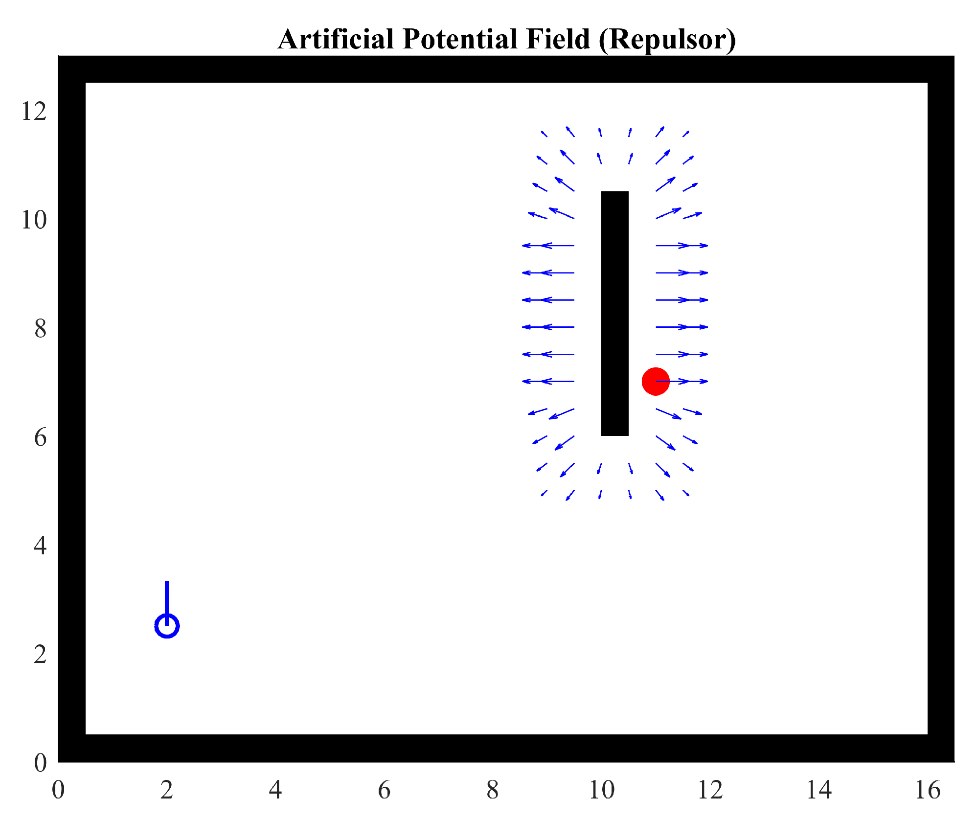
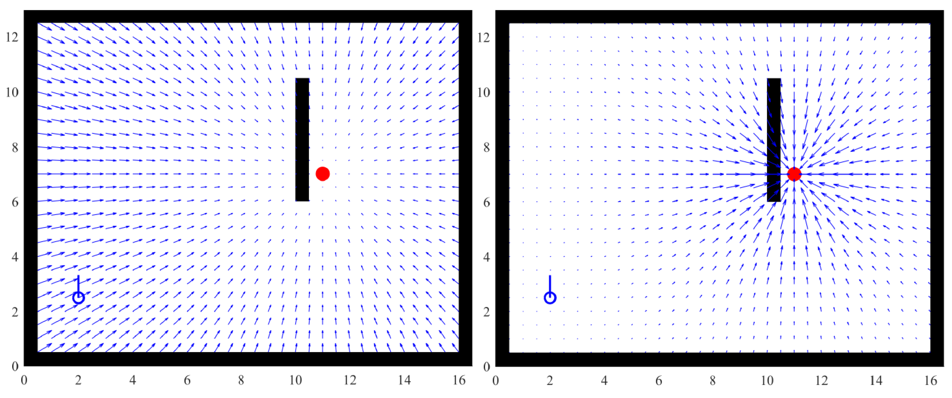
Figure 1 shows a wall in black with a target in red. The agent is represented in blue in the lower left corner. A field is generated by the potential function (Equation (4)) around the wall. This figure illustrates how the repulsive forces generated by the wall can potentially cause a local minimum and make it very challenging for the agent to reach its target. Note that the agent is outside the area of influence of the potential field, that is, the effect of the parameter.
where is the distance to the obstacle and is a limit that stops the field from progressing to infinity and eventually causing a division by 0. Parameter k is a constant that allows the adjustment of the generated field’s magnitude, while (Equation (4)) is a simplification of (Equation (3)) with similar behavior.
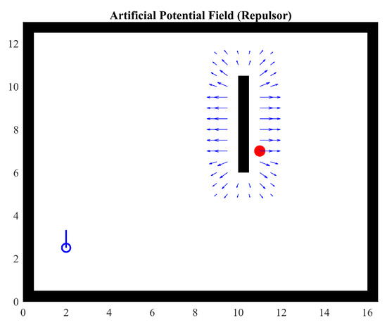
Figure 1.
Repulsor field generated by a wall. , .
The aforementioned functions show two fundamental features that are not always useful. Equation (2) grows rapidly with distance; therefore, a velocity control is needed. Equation (3) can yield forces as high as needed to avoid the obstacle. Although such behavior is desired, it is not suitable for any application since actuators will eventually saturate or even be destroyed. In case the agent’s actuators are not able to stop the movement, can reach the value 0 (Equation (4)), leading to a division-by-zero condition.
3.3. Proposed Potential Function
In order to merge the properties of the abovementioned functions but to avoid the downsides, the Agnesi function (Equation (5)) is proposed as a potential function. It is defined as follows:
If necessary, it can be expressed in more dimensions:
where and are unit vectors and for the two-dimensional case (Equation (6)). There is no limit for the number of dimensions. The operation of these equations in three-dimensional environments was documented in [18].
This function was introduced in The Treatise on Quadrature by Pierre Fermat in 1659. In 1703, Luigi Guido Grandi discussed the curve in Quadrature circuli et hyperbolae and named the curve as versoria. In 1748, Maria Gaetana Agnesi published Instituzioni analitiche ad uso della gioventù italiana and referred to the curve as versiera, a word that later would be erroneously translated as witch [38,39].
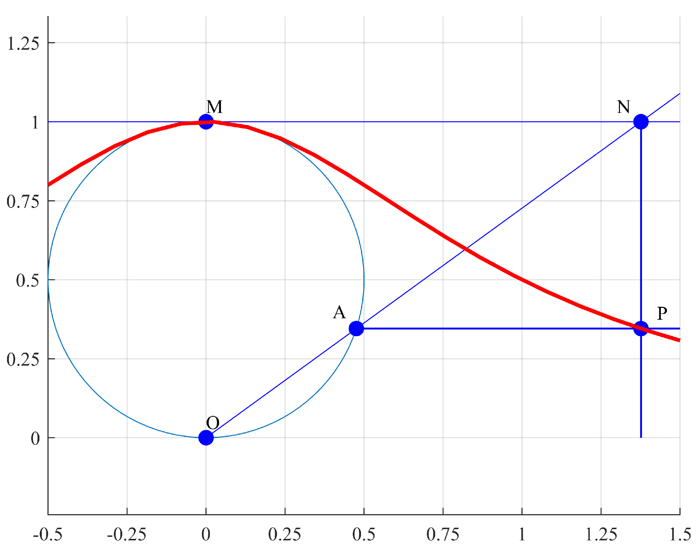
Geometrically, this curve is constructed with any two given points O and M. Diameter defines a circle. Given a point A in the circle, a secant line is drawn and extended up to the tangent line of the circle at point M. If a perpendicular line to that touches point A and a parallel line to through point N are drawn, then the intersection of both lines at point P defines the Agnesi curve. Constant a is the radius of the circle (see Figure 2).
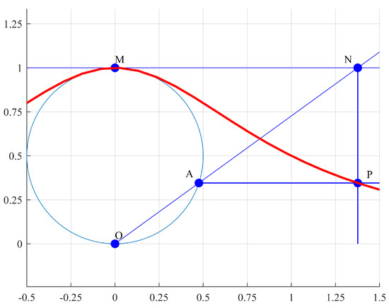
Figure 2.
Geometrical definition of the Agnesi curve.
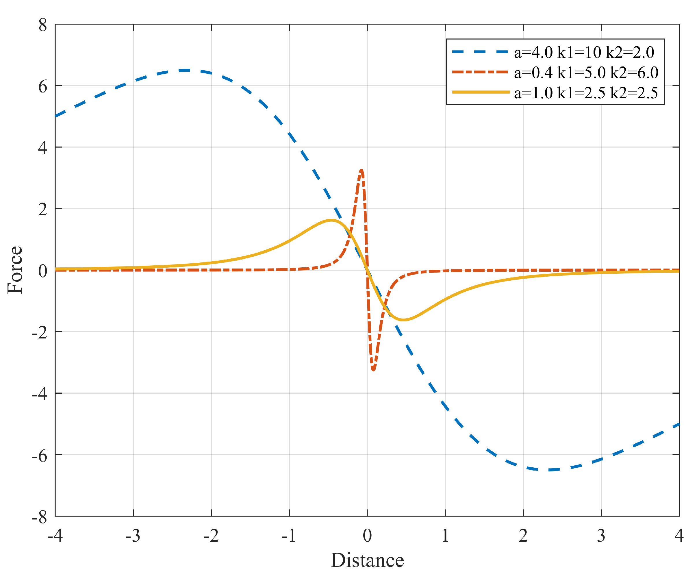
The Agnesi function is continuous and differentiable in the domain. Constants and (Equation (7)) are added to help control magnitude and width (Figure 3). With these modifications, the behavior of the square hyperbola can be achieved without the asymptote at 0.
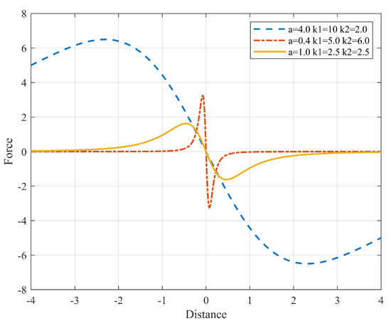
Figure 3.
Force generated in x using the Agnesi curve as a potential function.
Let and be position vectors; then, the error vector (Equation (8)) and its magnitude (Equation (9)) are defined as
Rewriting the Agnesi function (Equation (10)), we obtain
Thus, the generated force (Equations (11) and (12)) is given by
where and .
Figure 4 shows the difference between the fields produced by a quadratic function and the Agnesi curve. Notice that the influence zone of the field generated by the Agnesi curve is limited and that force decreases with distance, thereby reducing the possibility of creating undesired local minima. The field decreases rapidly to 0 at the target point. This feature is particularly useful for tracking, that is, keeping a distance from a moving object due to a strong field that keeps the agent close to the local minimum.
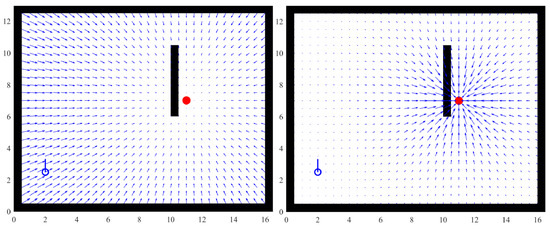
Figure 4.
APF comparison: using a quadratic function (Left), using the Agnesi curve (Right).
In contrast, a quadratic function creates a field that decreases gradually when the distance to the target decreases. This has two important consequences: first, if the agent is considerably far, the force will be high enough to produce undesired accelerations. Second, the force close to the target is low; thus, the agent can easily become deviated.
With this approach, it is possible to define different types of interactions by changing parameters a, and , guaranteeing that the field always exists in the domain, given that the potential function has no discontinuities. The modified Agnesi curve mentioned above can generate a smooth field leading to the target but avoiding the exponential growth with distance. Additionally, the exact same function can act as a barrier by modifying and . In that regard, it is easier to focus on behavior at a more abstract level.
Given the partial-observability constraints, the potential function proposed in this research is aimed to be used only locally. This feature is a differentiating factor from all other APF approaches implying that the AFP will be generated at a different point from the position of the main target, since the location of the latter is unknown. This is discussed in the following sections.
3.4. APF Parameters
Given all the above definitions, the a parameter has an important role within the proposed APF. Let us focus on the derivative of (Equation (13)):
3.4.1. Inflection Points
Inflection points can be used as a reference to define the region affected by the APF. Equations (14) and (15) show the second and third derivative of Equation (13), respectively:
In order to find the inflection points, let us set . Solving (Equation (15)) gives
It can be easily observed that there is an inflection point at , as expected. Solving the inner part of (Equation (17)), one can observed the existence of two more inflection points (Equation (18)):
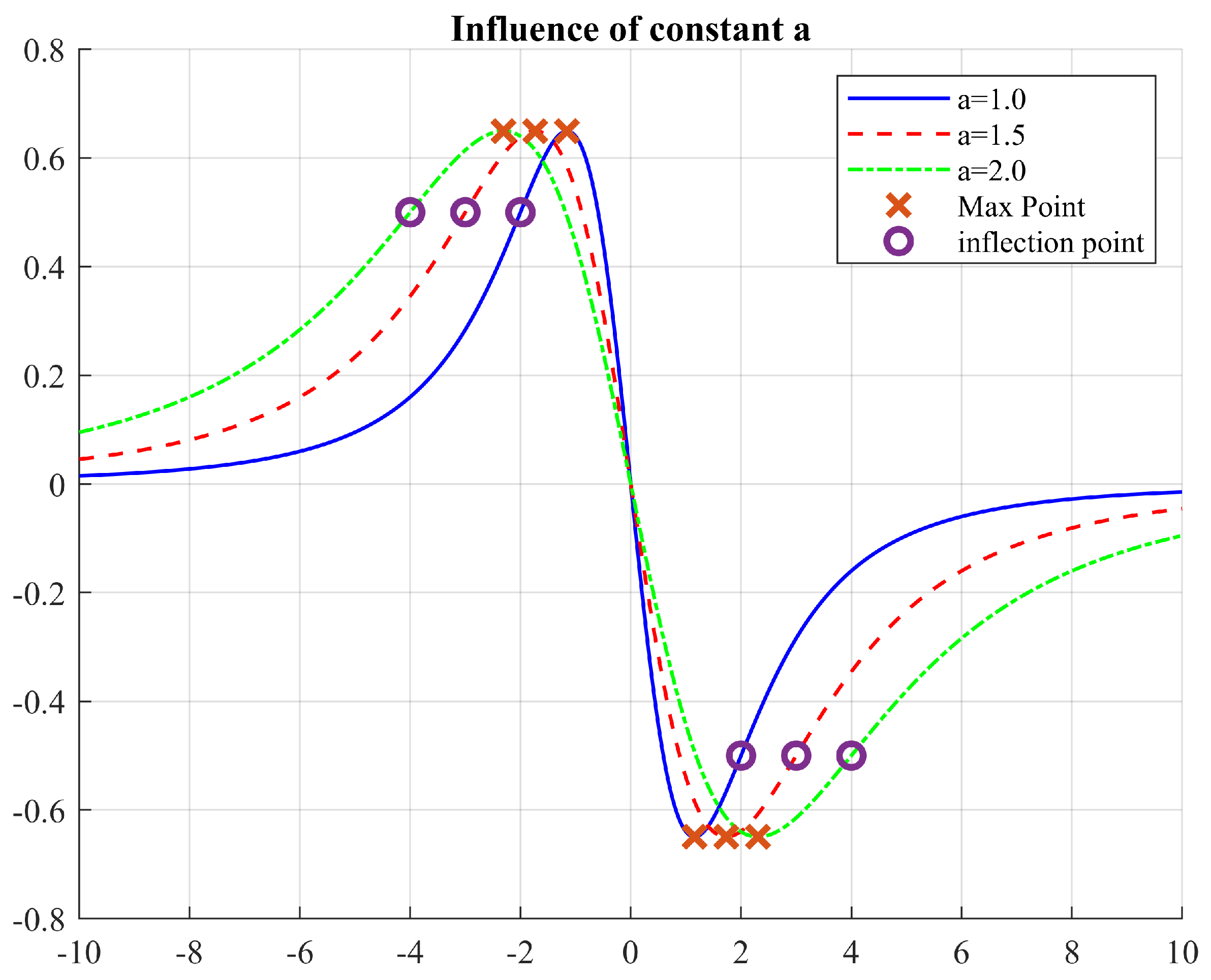
Parameter a will affect the position of the inflection points, but not their magnitude (Figure 5). Similarly, constant will only change the magnitude but not the position of the inflection points. Thus, these two parameters are independent and allow a fine tuning of the field’s scope of influence.
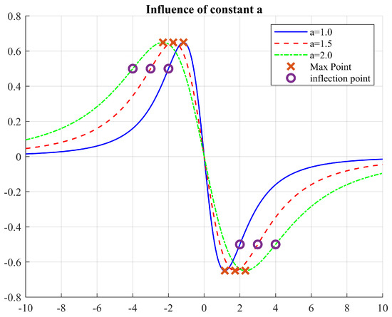
Figure 5.
Effect of changing the parameter a.
3.4.2. Maximum and Minimum Points
Alternatively, the maximum point, instead of the inflection points, can be used to find the max and min points. Let us set ; then, solving from Equation (14),
Thus, max and min points occur at
Notice that the maximum point position (Equation (21)) is also independent of (Figure 6). This has the potential to directly drive a with the known distance to the next target; however, acceleration will be directly affected and must be considered accordingly. The constant can be adjusted as necessary, depending on the intended response of the agent and the dynamics considerations. These observations are a matter of further study and are out of the scope of this work; therefore, the parameters remain constant in the simulations performed.
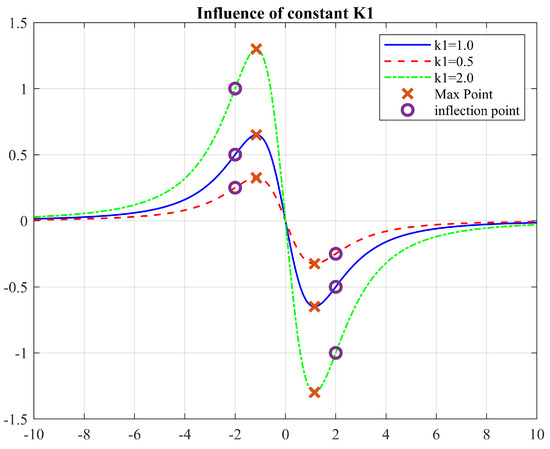
Figure 6.
Effect of changing the parameter .
3.5. Heuristics
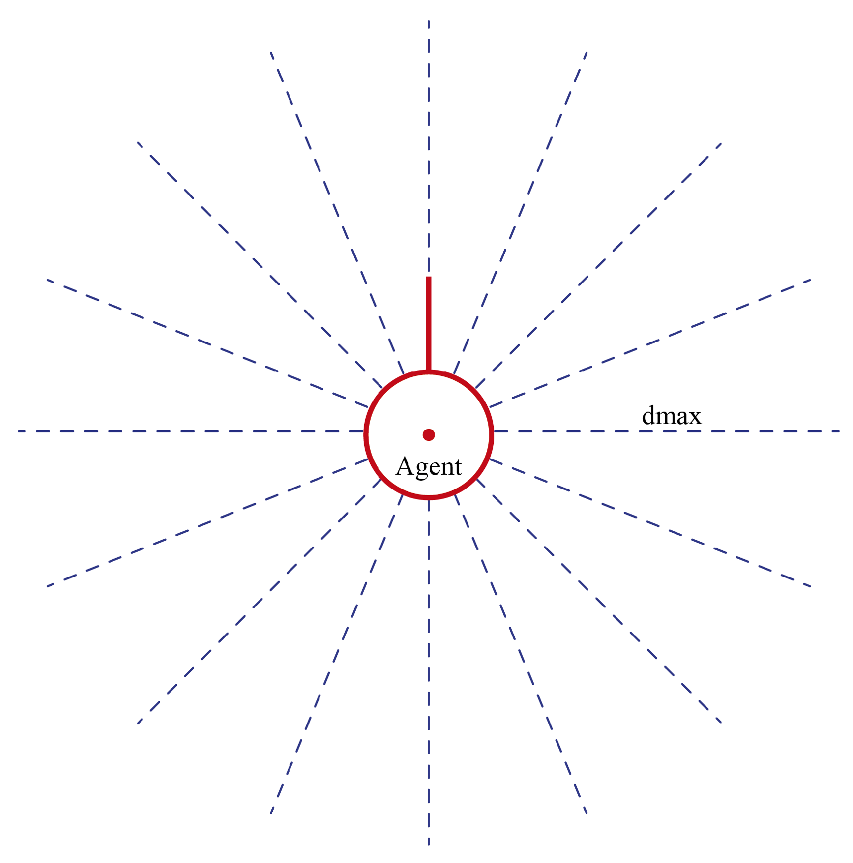
A direct consequence of partial observability is that the agent cannot determine the position of . However, middle points can be determined. Consider an agent with a field of view determined by , where is an angle and is the maximum distance that the agent can see. Let us also consider that the field of view is covered by n sensor beams, in order to emulate a LIDAR sensor (Figure 7). Under the above conditions, four states are defined:
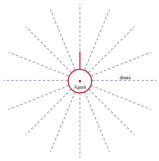
Figure 7.
Detection beams of the agent. The beams are equally distributed.
- Clear. No obstacles detected. A random angle and distance in the range and are selected.;
- Blocked. The readings of all sensors are less than ;
- Partially clear. One condition of interest is detected in . The angle and reading of the sensor are selected;
- Partially blocked. Obstacles are detected in any other condition different from the ones above.
is the minimum admissible distance for the agent to maneuver. The condition of interest is composed by some beam not detecting anything and at least one beam at its right and its left detecting something , where is the maximum possible reading when no objects are detected. Using these cases, it is possible to define middle target points.
Given the previous definitions, priorities can be assigned to each type of detection, so that the agent is able to turn the APFs on and off as needed. For instance, obstacles out of the collision course can be ignored in order to shorten the path to the next target.
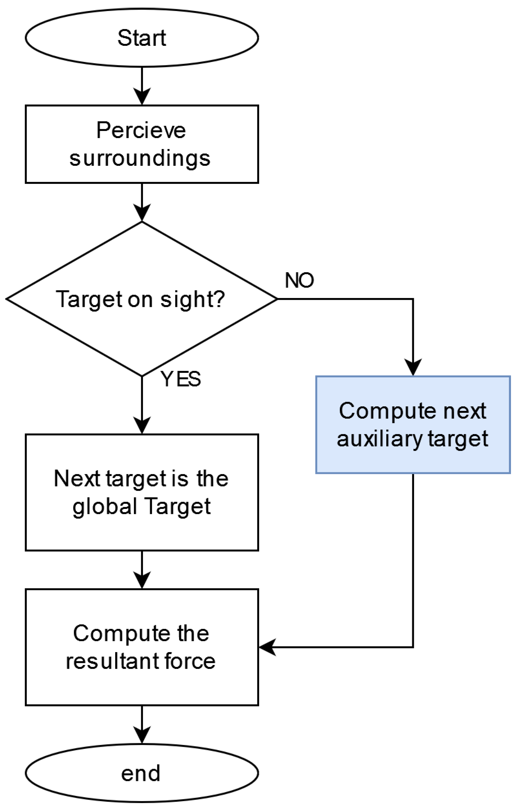
The above heuristics will determine where the next local target will be located. Its purpose is to provide a model (see Figure 8) that allow agents to navigate in an unknown environment under partial-observability constraints. Neither heuristics nor Artificial Potential Fields are capable of achieving this by themselves. However, when combined, the resulting model provide interesting capabilities. Notice that there is no path-planning process involved, since only one point ahead (local target) is computed each time.

Figure 8.
Process for computing the source point of the APF.
Most recent approaches [40,41,42] strongly rely on geometry, previous knowledge and modified versions of the classic potential functions. Only the availability of previous knowledge, either by communication or by perception, represents a challenge in any application scope. Thus, the ability to deal with partial-observability constraints is a feature that stands out.
3.6. Learning Process
The agent’s movement is driven by Artificial Potential Fields assisted by heuristics. During this process, points are generated. Such points can be used as input information for further processes. When the agent moves, a target point exists and a known point also exists. The difference is that the target point serves only as a guide to the movement and does not imply that it will be visited. On the other hand, a known point is the one that is visited and acquired by storing the current position of the agent.
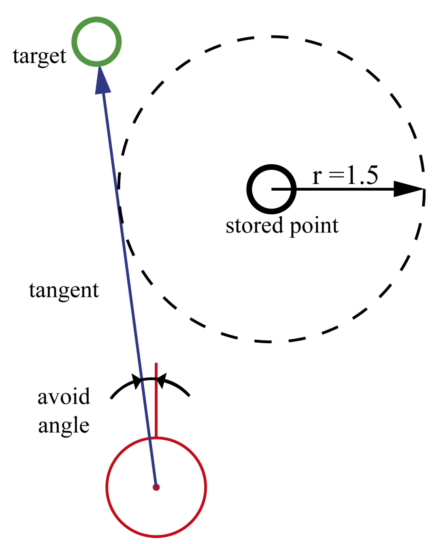
By storing the visited points, an exploration strategy can be implemented to avoid revisiting areas, for instance, by defining a circular zone around the visited points. When the agent is close to those areas, it will try to avoid their computation of the angle of a tangent to that zone (Figure 9). If the agent is too close to maneuver, then the point is ignored. Algorithm 1 shows these calculations. When the angle , the heuristics mentioned above work as described; otherwise, is used to determine the next target point.
| Algorithm 1: Avoid previously explored areas |
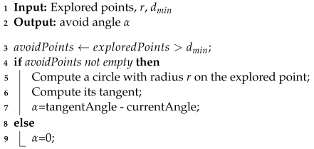 |
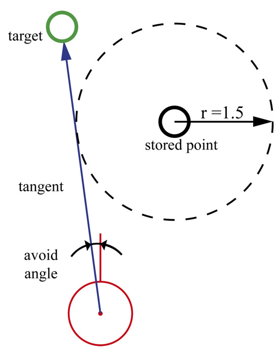
Figure 9.
Agent’s target computation while avoiding previously explored areas.
The ability to ignore stored points allows the agent to keep exploring without becoming stuck inside loops formed by visited points. The minimum distance and the radius r to ignore visited points are parameters of the exploration strategy.
While the agent explores, points that contribute to the exploration can be defined and the ones that have no meaning for the agent can be eliminated, for instance, dead ends. The above will result in two separate graphs: one containing the traveled path and one containing the points that lead to the current position of the agent. The aforementioned graphs are the result of the agent’s journey, not the result of previous computation. Therefore, there is no path or trajectory planning involved. The resultant graphs represent synthesized knowledge from the agent’s experience.
4. Experiments
All experiments were performed in MATLAB R2022b using the Mobile Robotics Simulation toolbox. The experimented scenarios were designed to contain specific challenging conditions:
- Passages: The agent must be able to navigate through gaps in the walls despite the repulsive forces from the side edges (scenario 1);
- Rooms: The agent must combine the skills of remembering previously visited areas with navigating through gaps in the walls, while avoiding becoming trapped in the central room (scenario 2);
- Hidden target: The agent’s exploration ability must be such as to allow it to find its target, even if it is deeply hidden in the environment (scenario 3);
- Open space: The agent must be able to navigate in open space, without prior knowledge of obstacles or the environment itself, and, at the same time, avoid previously explored areas (scenario 4).
All of the experiments are aimed at showing that the proposed model gives an agent, with no knowledge of the environment, the ability to navigate through it (explore) and eventually find its target.
4.1. Artificial Potential Fields in a Multi-Agent Environment
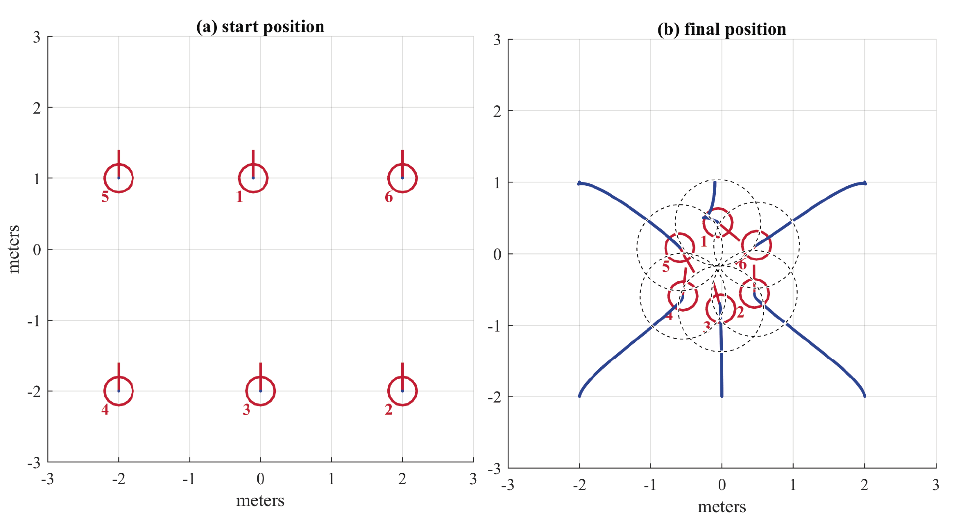
In order to verify the intended behavior of the APF, six agents where placed symmetrically with only one APF in order to keep a 1 m distance from the rest of the agents. The parameters used were , , .
In Figure 10 a the initial position of six numbered agents is shown. In Figure 10b, dotted lines describe 1 m diameter circles to verify that the condition of 1 m was met. The agents form a circle without having the explicit instruction of doing so. Each agent considers the force generated by all the agents in sight. As a consequence, the local minima are located 1 m away from the agents at the sides, but it is not possible to satisfy the 1 m condition regarding the other agents because that would imply a decrease in the distance between the closest agents. The result is an emergent stable formation.
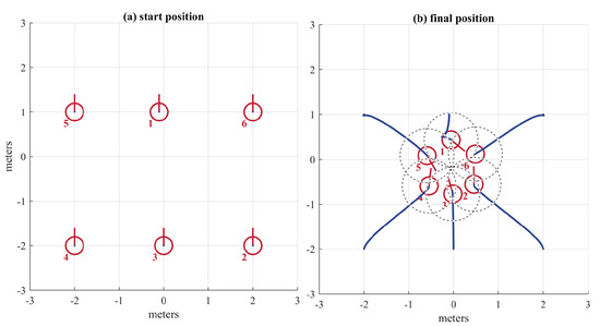
Figure 10.
(a) Start position (left). (b) Final position (right).
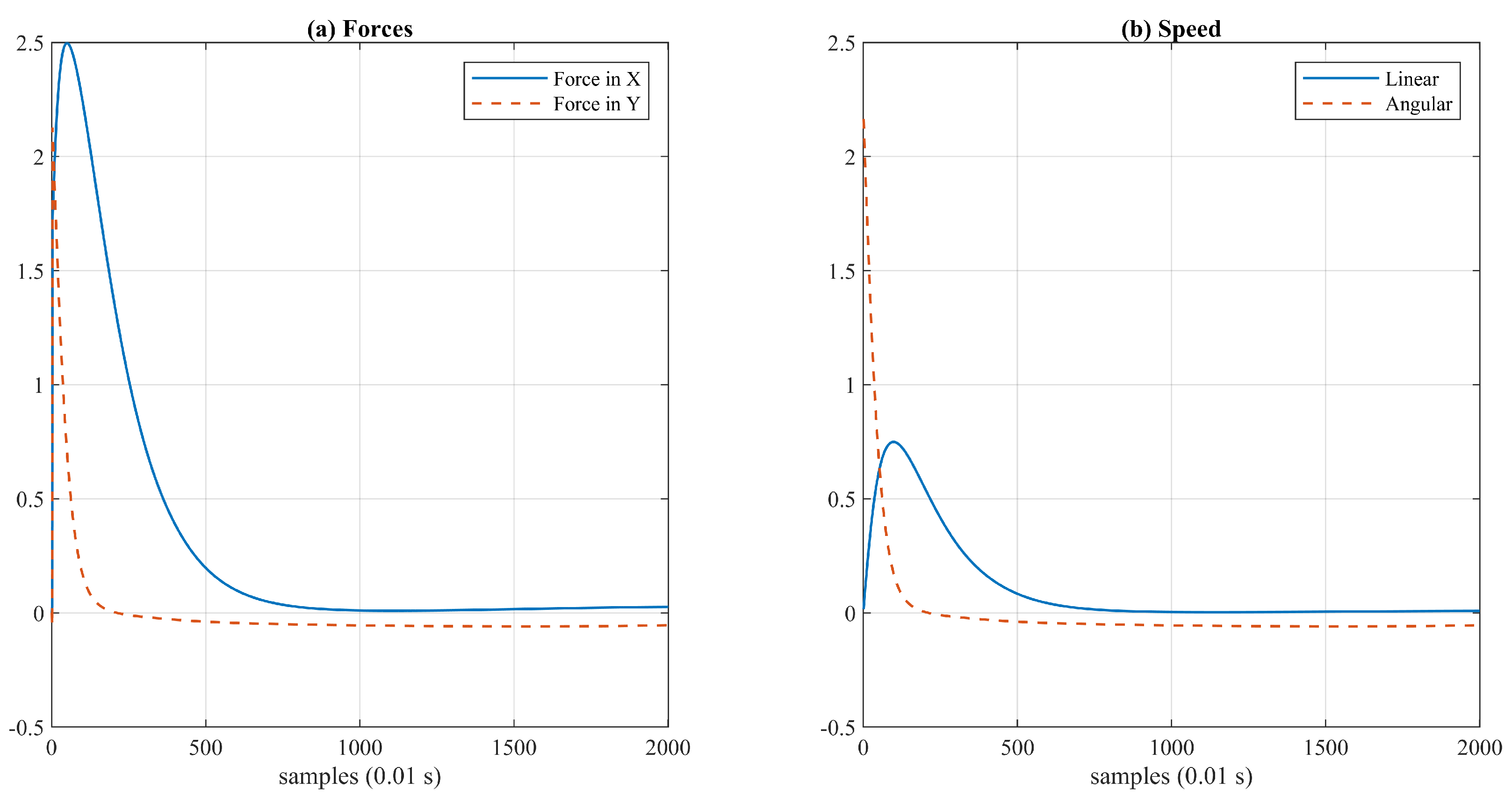
In Figure 11a, the resultant force on agent 2 is shown. Notice that the force is not 0; therefore, the agent is not exactly at the equilibrium point. However, it is close enough to generate forces too low to be able to cause movement in the agent. The effect of forces can be observed in Figure 11b, where the speed is almost 0. This result implies that, while it is true that agents can reach a stable formation., if the number of agents increases, the complexity in the interaction of forces also increases, yielding non-zero scenarios that must be considered in the heuristics. For instance, if the agent is in a local minimum but there are forces caused by agents located farther, the latter ones can be ignored to give priority to the closest ones.
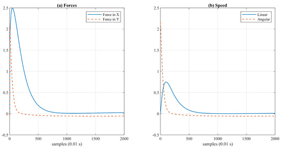
Figure 11.
Force and speed of agent number 2. (a) Forces, (b) Speed.
4.2. Scenario 1
An environment with straight walls is defined in order to assess the movement of the agent. The environment exposes the agent to the cases listed above to assess its behavior.
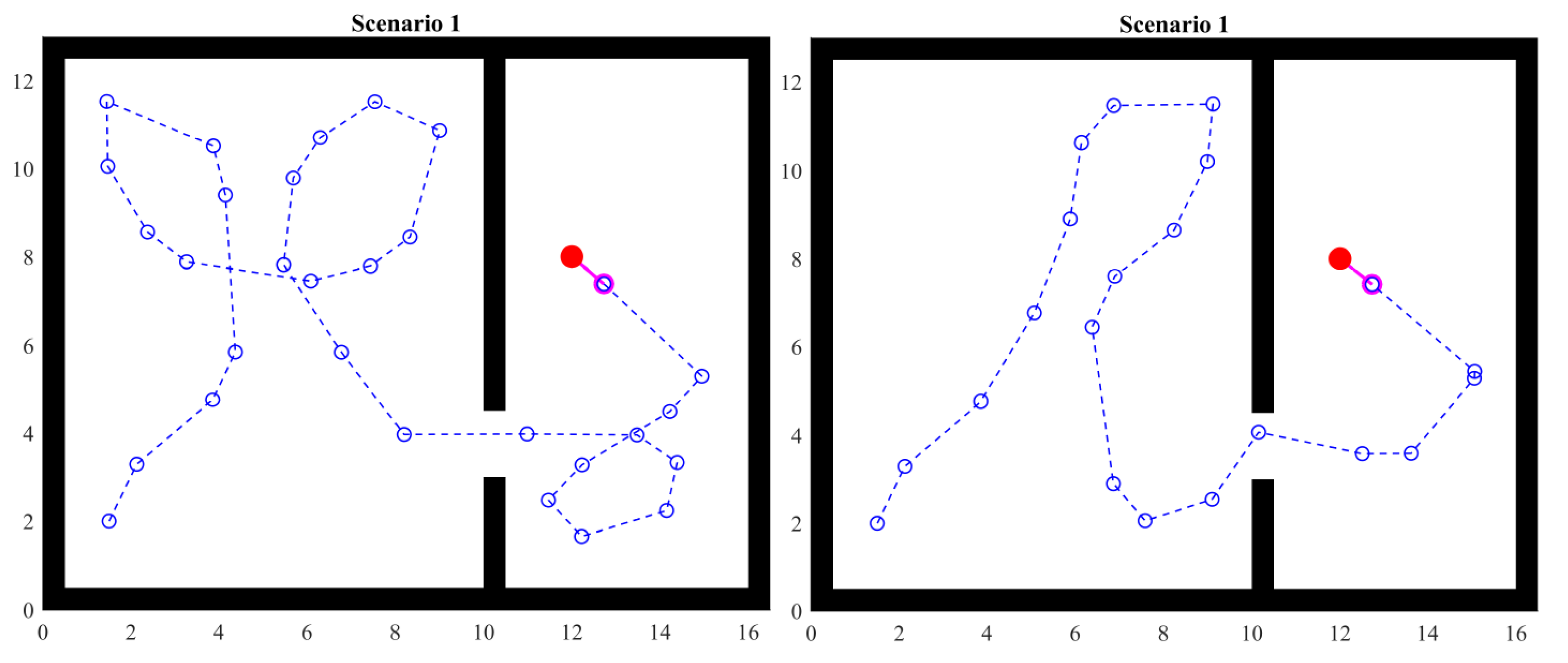
The left side of Figure 12 shows the traveled path with a dotted line. Circles are points visited by the agent. It can be observed that the path forms some loops. This experiment shows that, by storing the visited points, these are considered in the heuristics and avoid generating target points in the same positions, leading the agent effectively through the openings in the walls.

Figure 12.
Scenario 1: one passage.
Avoiding visited points helps the agent to move to unexplored regions as long as the space is sufficient. Otherwise, the agent will again pass over visited points, ignoring any avoiding strategy for the benefit of the ability to move. That is, the agent will avoid becoming stuck.
When the agent detects an interesting point, it will prioritize that direction over others. However, this also happens when the agent crosses the gap between the walls. Thus, it can go back. To avoid this behavior, visited points are used again. If the agent sees an interesting point and there is a visited point in that direction, it is then ignored and the next target will be positioned in an area with fewer obstacles. Notice that this overwrites the priority of avoiding visited points, given that the new target will ignore any of them.
The above shows that, according to the desired exploration strategy and the objective of the task to be performed, different priorities or rules can be established.
As mentioned in the previous section, random angles and distances are used when there is no further information. This is shown at the right side of Figure 12. The scenario and initial conditions are the same. However, the agent takes a different path.
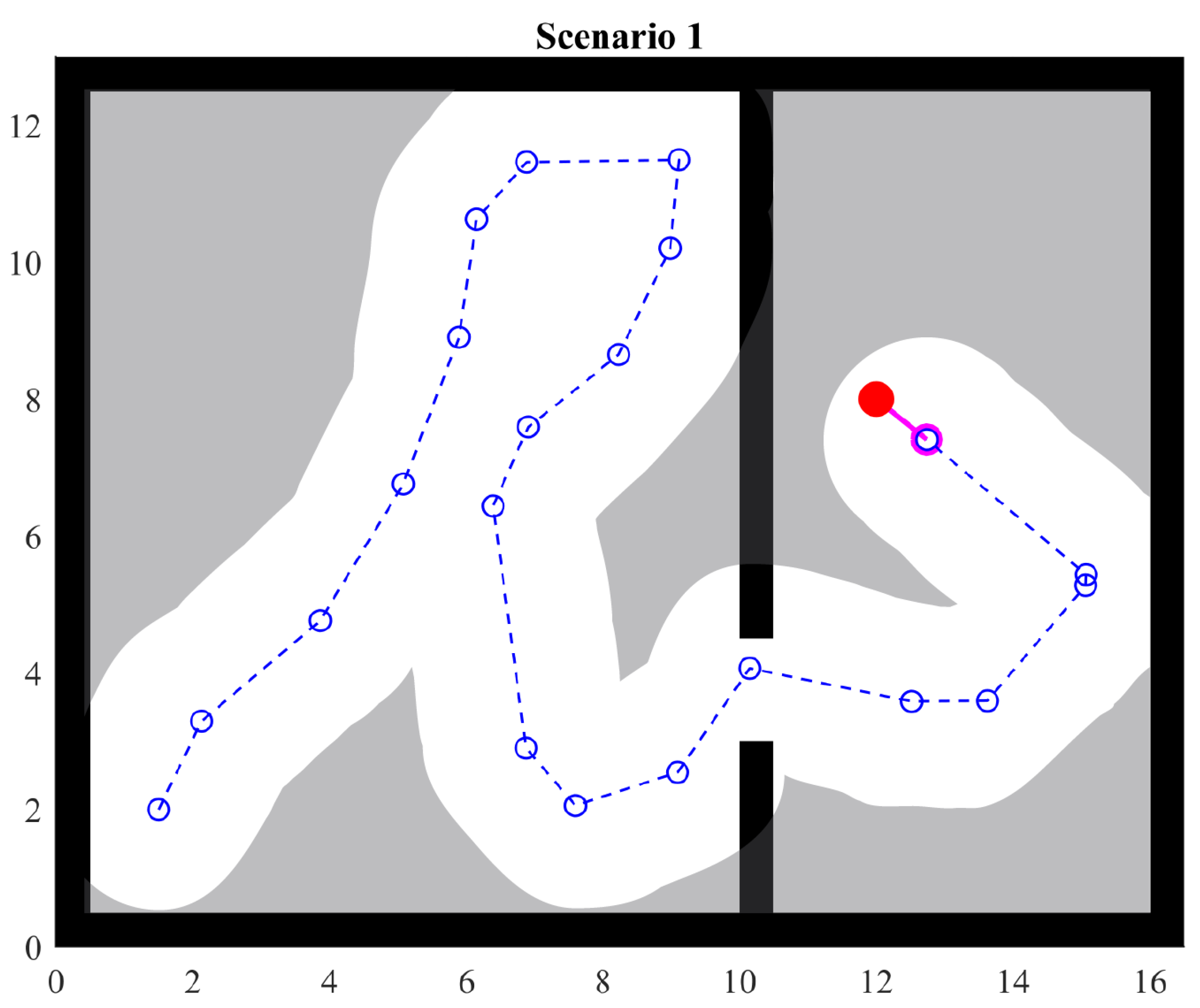
It is important to notice that the agent has a limited field of view; thus, the heuristics receive as input what the agent can see and the information stored in memory. Figure 13 shows the explored portion of the environment; gray regions are not known by the agent. When the agent finds the object, the set of visited points then forms a suitable route for the object and also contains a subset of points from which a better route can be built. Namely, the route can be optimized with the acquired knowledge, but this does not mean that a global optimum path can be found.
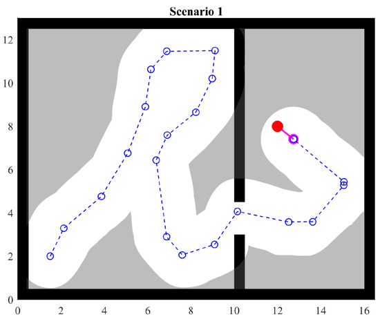
Figure 13.
Explored area.
4.3. Scenario 2
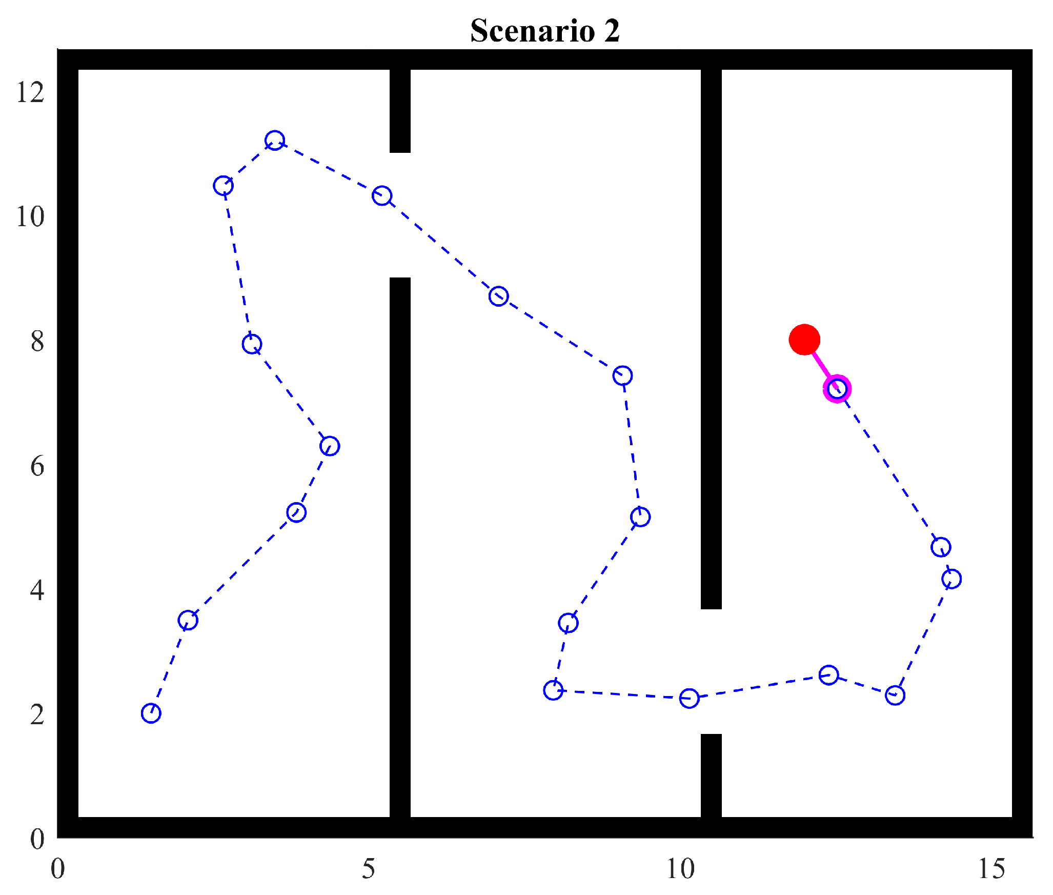
Scenario 2 provides two consecutive gaps between walls but in different positions, hence forcing the agent to search for the second gap. This can be seen as three rooms. In this case, the agent is temporarily enclosed in the second room because it does not have the starting point or the global target in sight. That is, it does not have any reference. In order to move and explore, the agent can only use the aforementioned heuristics and the stored points.
The experiment shows that the agent can find the object without any further issue, even when the simulation is run several times. This result exposes a clear behavior: when the agent has enough room to maneuver and is surrounded by walls close enough to always detect them, then the random factor considered in the heuristics has no effect, always yielding the same path.
Notice that heuristics provide a mechanism to adjust the exploration strategy. Since gaps in the wall are considered interesting points, the agent prioritizes exploring that region. Therefore, in a sense, heuristics encourage the agent to explore interesting points. Also, notice that, in Figure 14, the third room is barely explored since the object can be seen by the agent almost as soon as it enters the room. This condition is modified during the next experiment.
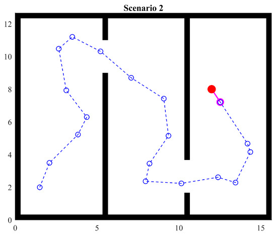
Figure 14.
Scenario 2: two passages.
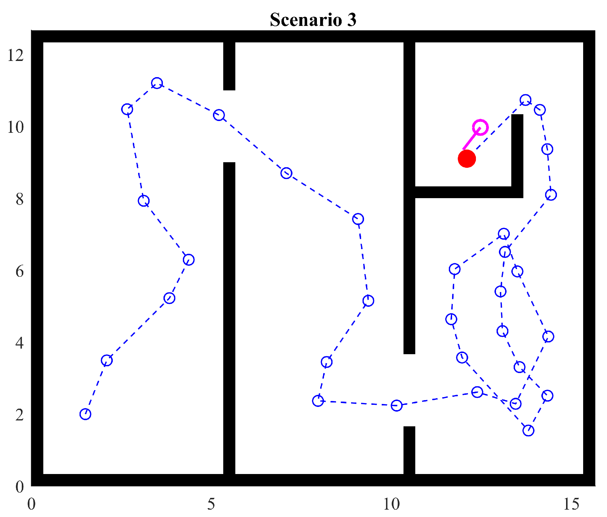
4.4. Scenario 3
In this experiment, the arrangement of the rooms and gaps in the walls is unchanged but the object is hidden behind walls (Figure 15). It can be observed that the navigation through the first two rooms remains the same; however, in the third room, the agent explores the zone until it eventually finds the final passage to the corner. As soon as the object is in sight, the agent moves to it.
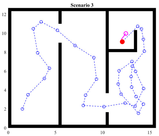
Figure 15.
Scenario 3: two passages with a hidden target point.
This scenario shows the ability to avoid returning across passages and moving to explore unexplored regions. It is important to highlight that the existence of the ability does not imply certainty in the behavior. In fact, Artificial Potential Fields with heuristics only provide certainty that the agent will explore unknown areas, but not necessarily all of them since the agent will stop when the target point is reached, which is a basic behavior.
As the complexity of a scenario increases, the ability to choose the convenient type of Artificial Potential Field become more relevant. Heuristics can decide which APF is better. For example, to move closer to a very distant point, a quadratic potential function is used, while, for avoiding collisions at all costs, a hyperbolic function is more convenient.
It is worth highlighting that the location of the next target point impacts changes in the APF used. Since reachable points close to the agent are prioritized, heuristics can be viewed as optimizing the use of APFs. Consequently, changes in the used APF type will tend to be low.
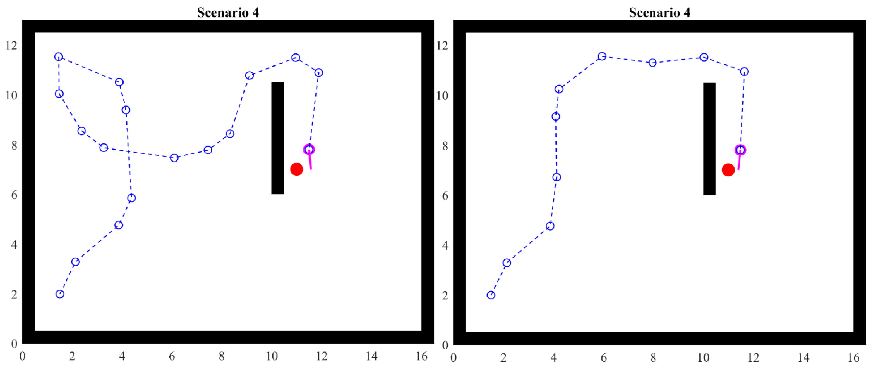
4.5. Scenario 4
When the agent has a space such that there is no reference close to it to decide the direction, the random selection of angle and distance will then take relevance. This scenario shows what happens under those circumstances.
Two examples are shown. Figure 16 shows that different executions of the simulation can yield different paths to the objective. It may seem tempting to think that one route is better or optimal in some way; however, this is only the result of random choices that lead to specific cases such as finding walls or corners. It is important to keep in mind that, from the point of view of the agent, there is no metric to optimize or decide that some actions are better than others. However, since visited points are represented in each agent’s memory, that knowledge can have further use, including optimization. When we as humans see the complete scenario, we make inferences that the agent would not make. Therefore, APFs with heuristics are only a basis that provides the ability to explore an unknown partially observable scenario.
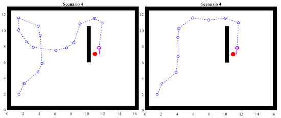
Figure 16.
Scenario 4: one obstacle.
5. Conclusions
In this paper, we have shown that merging Artificial Potential Fields (APF) with search heuristics yields an effective and efficient algorithmic combination for navigation scenarios and exploration tasks. Using the Agnesi curve as potential function allows the effect of APF to be bounded in order to reduce the possibility of generating unintended local minima and increasing the influence of the fields in the desired scope, thus increasing its effectiveness. The price to pay for the ability to control the APF as described in this paper is an increase in the number of parameters for each field, as well as the need for careful setting of each parameter.
The APF approach, together with a fine control of the scope of influence provided by the curve of Agnesi, allows agents to be modeled as simple points, despite the kinematics and dynamics involved. This turns out to be useful for further abstraction in the design of the agent’s behavioral models.
Given the conditions of partial observability, the next target point of an agent can only be defined locally; therefore, a mechanism is required for determining the location of that point. Heuristics provide such a mechanism, allowing the definition of that point based on the agent’s perception. Particularly relevant in such perception tasks are the directions that are blocked and those that are clear. Simulations show that an agent using APF, with its local knowledge about blocked and free directions, is still able to explore by choosing a direction with fewer obstacles. The ability to make those decisions has the potential to serve as a foundation for the design of more intelligent and autonomous agents, though more research is needed.
When there is no information about nearby obstacles, the auxiliary heuristics choose a random direction, which is a clear obstacle to studying the repeatability of the agent’s behavior. An important limitation of this model is that the reachability of the target is not ensured. The heuristics are not enough to ensure that the agent will continue navigating and avoiding already-explored areas until reaching the target. This is especially true when the number of explored points increases; in such situations, the agent should decide which areas are not worth exploring and which areas are needed in order to continue the exploration of unknown areas and the search for the target. To address the above, a mapping algorithm alongside an environmental representation is needed.
The APF/heuristics combination allows the agent navigation to be smooth, yielding an exploration behavior that does not require any pauses, even in a partially observable environment, because navigation points are continuously computed. Additionally, heuristics allow specific locations such as openings in the walls to be processed as specific situations, allowing the agent to gather and produce more knowledge about those points and increasing the agent’s ’curiosity’ to explore those locations in greater detail.
6. Future Work
As the proposed model does not rely on geometry features or previous knowledge, it reduces the number of computational steps for the next local target and introduces new features such as the scope of influence of the APF and a decision-making stage. All introduced features have the potential to serve as the basis for behavioral models in intelligent agents. As a result, agents can now be modeled as decision-makers and not just as trajectory/path planners. More research is required in that regard.
Experimental results provide an insight into what can be achieved if other layers of behavior and/or knowledge abstraction are added to the agent. Agents begin each navigation task only with the ability to perceive points in the environment, and a first layer of APF-guided collision-free navigation allows them to explore the environment. But, as they explore, they could also synthesize the knowledge about already-explored points and create routes and maps. Such adaptation comes from the use of Artificial Potential Fields, and this is another related line of research that our team is addressing.
It seems feasible and relevant to explore the creation of a swarm of decision-making agents. The ability to take actions based on what they perceive has the potential to lead to highly adaptive agents. And adding more agents and considering the possibilities for sharing knowledge between them seems an equally interesting area of research.
Our next step is to provide a structure and protocol for the collection and communication of knowledge between the agents of a swarm. Shared knowledge can then be used as an input in posterior cognition and reasoning stages of each agent. The addition of these stages can lead to the development of layered behavioral models, as mentioned before. Each layer increases the level of abstraction in the agent’s reasoning and enables the development of different types of behavioral skills.
The ability to represent the knowledge acquired by an agent is important for planning and executing exploration and search tasks. Constructing a collective knowledge base that contains all information gathered from the perceptual stages of an agent also seems to be a path that is worth exploring.
Author Contributions
Conceptualization, methodology, software, investigation, witting: D.S.C. Supervision, review and editing: S.G.-C. All authors have read and agreed to the published version of the manuscript.
Funding
This research was funded by Consejo Nacional de Humanidades Ciencias y Tecnologías (CONAHCYT) and Secretaría de Investigación y Posgrado (SIP-IPN) through grant SIP-20241315.
Institutional Review Board Statement
Not applicable.
Informed Consent Statement
Not applicable.
Data Availability Statement
The raw data supporting the conclusions of this article will be made available by the authors on request.
Acknowledgments
The authors wish to thank Consejo Nacional de Humanidades Ciencias y Tecnologías (CONAHCYT) and Instituto Politécnico Nacional, Secretaría de Investigación y Posgrado (SIP-IPN) for their support of this research through project SIP-20241315.
Conflicts of Interest
The authors declare no conflicts of interest.
References
- Holland, O. Exploration and high adventure: The legacy of Grey Walter. Philos. Trans. Ser. Math. Phys. Eng. Sci. 2003, 361, 2085–2121. [Google Scholar] [CrossRef] [PubMed]
- Walter, W.G. An Electro-Mechanical «Animal». Dialectica 1950, 4, 206–213. [Google Scholar] [CrossRef]
- Nilsson, N.J. Shakey the Robot. In Proceedings of the Technical Note No. 323; SRI International: Menlo Park, CA, USA, 1984. [Google Scholar]
- Sun, K.; Schlotfeldt, B.; Pappas, G.J.; Kumar, V. Stochastic Motion Planning Under Partial Observability for Mobile Robots With Continuous Range Measurements. IEEE Trans. Robot. 2021, 37, 979–995. [Google Scholar] [CrossRef]
- Elhoseny, M.; Tharwat, A.; Hassanien, A.E. Bezier Curve Based Path Planning in a Dynamic Field using Modified Genetic Algorithm. J. Comput. Sci. 2018, 25, 339–350. [Google Scholar] [CrossRef]
- Patle, B.; Babu L, G.; Pandey, A.; Parhi, D.; Jagadeesh, A. A review: On path planning strategies for navigation of mobile robot. Def. Technol. 2019, 15, 582–606. [Google Scholar] [CrossRef]
- Khatib, O.; Le Maitre, J.-F. Dynamic Control of Manipulators Operating in a Complex Environment. In Proceedings of the 3rd CISM-IFToMM Symposium on Theory and Practice of Robots and Manipulators, Udine, Italy, 12–15 September 1978; pp. 267–282. [Google Scholar]
- Khatib, O. Dynamic Control of Manipulator in Operational Space. In Proceedings of the 6th IFToMM World Congress on Theory of Machines and Mechanisms, New Delhi, India, 15–20 December 1983. [Google Scholar]
- Khatib, O. Real-time obstacle avoidance for manipulators and mobile robots. In Proceedings of the 1985 IEEE International Conference on Robotics and Automation, St. Louis, MO, USA, 25–28 March 1985; Volume 2, pp. 500–505. [Google Scholar] [CrossRef]
- Khatib, O. The Potential Field Approach And Operational Space Formulation In Robot Control. In Adaptive and Learning Systems: Theory and Applications; Narendra, K.S., Ed.; Springer: Boston, MA, USA, 1986; pp. 367–377. [Google Scholar] [CrossRef]
- Khatib, O. The Operational Space Formulation in Robot Manipulator Control. In Proceedings of the 15th International Symposium on Industrial Robots, Tokyo, Japan, 11–13 September 1985; pp. 165–172. [Google Scholar]
- Barnes, L.; Fields, M.; Valavanis, K. Unmanned ground vehicle swarm formation control using potential fields. In Proceedings of the 2007 Mediterranean Conference on Control Automation, Athens, Greece, 27–29 June 2007; pp. 1–8. [Google Scholar] [CrossRef]
- Barnes, L.E.; Fields, M.A.; Valavanis, K.P. Swarm Formation Control Utilizing Elliptical Surfaces and Limiting Functions. IEEE Trans. Syst. Man, Cybern. Part (Cybern.) 2009, 39, 1434–1445. [Google Scholar] [CrossRef]
- Fan, X.; Guo, Y.; Liu, H.; Wei, B.; Lyu, W. Improved Artificial Potential Field Method Applied for AUV Path Planning. Math. Probl. Eng. 2020, 2020, 1–21. [Google Scholar] [CrossRef]
- Wang, S.; Zhao, T.; Li, W. Mobile Robot Path Planning Based on Improved Artificial Potential Field Method. In Proceedings of the 2018 IEEE International Conference of Intelligent Robotic and Control Engineering (IRCE), Lanzhou, China, 24–27 August 2018. [Google Scholar] [CrossRef]
- Tao, S. Improved artificial potential field method for mobile robot path planning. Appl. Comput. Eng. 2024, 33, 157–166. [Google Scholar] [CrossRef]
- Arkin, R. Motor schema based navigation for a mobile robot: An approach to programming by behavior. In Proceedings of the the 1987 IEEE International Conference on Robotics and Automation, Raleigh, NC, USA, 31 March–3 April 1987; Volume 4, pp. 264–271. [Google Scholar] [CrossRef]
- Silva, D.; Leal, M.A.; Dorantes, E. Diseño e Implementación de un Sistema de Visión estéReo Para Controlar un Robot Antropomórfico en el Espacio Tarea. Bachelor’s Thesis, Unidad Profesional Interdisciplinaria en Ingeniería y Tecnologías Avanzadas—National Polytechnic Institute, Mexico, Mexico, 2012. (In Spanish). [Google Scholar]
- Koditschek, D.E. Exact robot navigation by means of potential functions: Some topological considerations. In Proceedings of the 1987 IEEE International Conference on Robotics and Automation, Raleigh, NC, USA, 31 March–3 April 1987; Volume 4, pp. 1–6. [Google Scholar] [CrossRef]
- Koditschek, D.E. Natural Motion for Robot Arms. In Proceedings of the 23rd IEEE Conference on Decision and Control, Las Vegas, NV, USA, 12–14 December 1984. [Google Scholar] [CrossRef]
- Park, M.; Lee, M.C. A new technique to escape local minimum in artificial potential field based path planning. J. Mech. Sci. Technol. 2003, 17, 1876–1885. [Google Scholar] [CrossRef]
- Choi, W.; Latombe, J.C. A reactive architecture for planning and executing robot motions with incomplete knowledge. In Proceedings of the IROS ’91:IEEE/RSJ International Workshop on Intelligent Robots and Systems ’91, Osaka, Japan, 3–5 November 1991; pp. 24–29. [Google Scholar] [CrossRef]
- Borenstein, J.; Koren, Y. Real-Time Obstacle Avoidance for Fast Mobile Robots. Syst. Man Cybern. IEEE Trans. 1989, 19, 1179–1187. [Google Scholar] [CrossRef]
- Zhang, T.; Zhu, Y.; Song, J. Real-Time Motion Planning for Mobile Robots by Means of Artificial Potential Field Method in Unknown Environment. Ind. Robot. Int. J. 2010, 37, 384–400. [Google Scholar] [CrossRef]
- Zhang, Y.; Chen, J.; Chen, M.; Chen, C.; Zhang, Z.; Deng, X. Integrated the Artificial Potential Field with the Leader–Follower Approach for Unmanned Aerial Vehicles Cooperative Obstacle Avoidance. Mathematics 2024, 12, 954. [Google Scholar] [CrossRef]
- Zhao, W.; Li, L.; Wang, Y.; Zhan, H.; Fu, Y.; Song, Y. Research on A Global Path-Planning Algorithm for Unmanned Arial Vehicle Swarm in Three-Dimensional Space Based on Theta*–Artificial Potential Field Method. Drones 2024, 8, 125. [Google Scholar] [CrossRef]
- Lu, S.; Xu, R.; Li, Z.; Wang, B.; Zhao, Z. Lunar Rover Collaborated Path Planning with Artificial Potential Field-Based Heuristic on Deep Reinforcement Learning. Aerospace 2024, 11, 253. [Google Scholar] [CrossRef]
- Sun, J.; Tang, J.; Lao, S. Collision Avoidance for Cooperative UAVs With Optimized Artificial Potential Field Algorithm. IEEE Access 2017, 5, 18382–18390. [Google Scholar] [CrossRef]
- Zhou, Z.; Wang, J.; Zhu, Z.; Yang, D.; Wu, J. Tangent navigated robot path planning strategy using particle swarm optimized artificial potential field. Opt.-Int. J. Light Electron Opt. 2017, 158, 639–651. [Google Scholar] [CrossRef]
- Zheng, L.; Yu, W.; Li, G.; Qin, G.; Luo, Y. Particle Swarm Algorithm Path-Planning Method for Mobile Robots Based on Artificial Potential Fields. Sensors 2023, 23, 6082. [Google Scholar] [CrossRef] [PubMed]
- Orozco-Rosas, U.; Montiel, O.; Sepúlveda, R. Mobile robot path planning using membrane evolutionary artificial potential field. Appl. Soft Comput. 2019, 77, 236–251. [Google Scholar] [CrossRef]
- Weerakoon, T.; Ishii, K.; Nassiraei, A. An Artificial Potential Field Based Mobile Robot Navigation Method to Prevent from Deadlock. J. Artif. Intell. Soft Comput. Res. 2015, 5, 189–203. [Google Scholar] [CrossRef]
- Chen, X.; Kong, Y.; Fang, X.; Wu, Q. A fast two-stage ACO algorithm for robotic path planning. Neural Comput. Appl. 2013, 22, 313–319. [Google Scholar] [CrossRef]
- Bai, J.; Chen, L.; Jin, H.; Chen, R.; Mao, H. Robot path planning based on random expansion of ant colony optimization. In Recent Advances in Computer Science and Information Engineering: Volume 2; Springer: Berlin/Heidelberg, Germany, 2012; pp. 141–146. [Google Scholar]
- Wang, Y.; Chen, P.; Jin, Y. Trajectory planning for an unmanned ground vehicle group using augmented particle swarm optimization in a dynamic environment. In Proceedings of the 2009 IEEE International Conference on Systems, Man and Cybernetics, Antonio, TX, USA, 11–14 October 2009; pp. 4341–4346. [Google Scholar]
- Hao, Y.; Zu, W.; Zhao, Y. Real-time obstacle avoidance method based on polar coordination particle swarm optimization in dynamic environment. In Proceedings of the 2007 2nd IEEE conference on industrial electronics and applications, Harbin, China, 23–25 May 2007; pp. 1612–1617. [Google Scholar]
- Dolgov, D.; Thrun, S.; Montemerlo, M.; Diebel, J. Path Planning for Autonomous Vehicles in Unknown Semi-structured Environments. I. J. Robot. Res. 2010, 29, 485–501. [Google Scholar] [CrossRef]
- Truesdell, C. Maria Gaetana Agnesi. Arch. Hist. Exact Sci. 1989, 40, 113–142. [Google Scholar] [CrossRef]
- Larsen, H.D. The witch of agnesi. Sch. Sci. Math. 1946, 46, 57–62. [Google Scholar] [CrossRef]
- Zhai, L.; Liu, C.; Zhang, X.; Wang, C. Local Trajectory Planning for Obstacle Avoidance of Unmanned Tracked Vehicles Based on Artificial Potential Field Method. IEEE Access 2024, 12, 19665–19681. [Google Scholar] [CrossRef]
- Samodro, M.; Dp, R.; Caesarendra, W. Artificial Potential Field Path Planning Algorithm in Differential Drive Mobile Robot Platform for Dynamic Environment. Int. J. Robot. Control. Syst. 2023, 3, 161–170. [Google Scholar] [CrossRef]
- Melchiorre, M.; Salamina, L.; Scimmi, L.S.; Mauro, S.; Pastorelli, S. Experiments on the Artificial Potential Field with Local Attractors for Mobile Robot Navigation. Robotics 2023, 12, 81. [Google Scholar] [CrossRef]

Disclaimer/Publisher’s Note: The statements, opinions and data contained in all publications are solely those of the individual author(s) and contributor(s) and not of MDPI and/or the editor(s). MDPI and/or the editor(s) disclaim responsibility for any injury to people or property resulting from any ideas, methods, instructions or products referred to in the content. |
© 2024 by the authors. Licensee MDPI, Basel, Switzerland. This article is an open access article distributed under the terms and conditions of the Creative Commons Attribution (CC BY) license (https://creativecommons.org/licenses/by/4.0/).