Proximity-Based Adaptive Indoor Positioning Method Using Received Signal Strength Indicator

Abstract

In this paper, we propose a proximity-based adaptive positioning algorithm to address the challenge of positioning errors in indoor localization based on RSSI (received signal strength indicator). When positioning by trilateration, if a receiver is close to one AP, the signals of other APs become rapidly unstable, so positioning accuracy is reduced. Therefore, this paper proposes an algorithm to identify the proximity state with AP and adaptively determine the positioning technique based on this state. The proposed algorithm consists of three steps: RSSI error correction, adaptive location estimation, and post-processing. The RSSI error correction step corrects unstable RSSI. The adaptive location estimation step utilizes a modified proximity technique when identified as close to an AP, employing trilateration otherwise. Finally, in the post-processing step, an efficient filtering algorithm is applied. For the static state experiment, the accuracy of the proposed algorithm is found to be improved by about 28% compared to the method measured using only the trilateration technique applying the RSSI error correction step and post-processing step. The proposed algorithm improved the positioning accuracy of the entire area by improving accuracy in regions with weak signals without additional devices.

1. Introduction

Recent advances in wireless communication technology have increased the demand for LBS (location-based services) that provide location-specific information. The positioning technology of LBS is applied to various fields such as navigation, inventory management, access security, crowd management, and disaster rescue [1,2,3,4,5]. Location positioning can be categorized into outdoor and indoor positioning based on an individual’s location. Outdoor locations can be accurately determined mainly using GPS (global positioning system) [6]. However, GPS-based positioning encounters disruptions in underground or enclosed spaces and exhibits an error of approximately tens of meters, making it unsuitable for indoor positioning [7,8]. To achieve precise indoor positioning, it is necessary to utilize wireless signals with high accuracy [9].

There are various positioning techniques for indoor environments, such as geomagnetism [10], UWB (ultra—wideband) [11,12], BLE (bluetooth low energy), and Wi-Fi signals. The technique of indoor positioning using geomagnetism involves constructing a map of the magnetic field distribution to determine location. The advantage is that no additional equipment is required, but the disadvantage is that it requires preliminary work to create the map. Moreover, its application becomes challenging in environments with local magnetic disturbances, such as those encountered in subway systems, leading to variations in magnetic field distribution. UWB wireless communication technology demonstrates high accuracy in indoor positioning systems because it operates in ultra-wideband frequencies with high penetration characteristics. However, considerations such as the elevated installation cost and potential electromagnetic interference risks due to a wide bandwidth should be addressed. BLE or Wi-Fi-based indoor positioning techniques exhibit low precision and accuracy because of vulnerability to interference such as reflection, refraction, diffraction, and scattering. Nevertheless, its economic advantages, low computational complexity, and high availability make advantages for efficient indoor positioning.

Indoor positioning techniques using BLE or Wi-Fi include fingerprinting techniques [13] and trilateration technique [14,15]. Indoor positioning through fingerprinting involves collecting signal patterns at regular intervals within the desired region, constructing a signal distribution map, and estimating the location based on the similarity between the collected and measured signal patterns [13]. With advancement of artificial intelligence, AI-based approaches have been proposed for fingerprinting-based indoor positioning [16,17]. Learning-based indoor positioning techniques such as machine learning and deep learning utilize signal data collected from sensors at various reference points to train an optimal model connecting measured values and estimated final positions [18]. AI-based fingerprinting techniques excel at identifying complex, non-linear patterns, resulting in improved positioning accuracy compared to traditional fingerprinting approaches [17]. However, the burden of pre-work and the increase in computational complexity proportional to the region to be placed cause disadvantages. Additionally, AI-based fingerprinting depends heavily on pre-collected signal patterns, making it difficult to adapt to changing environmental conditions, requiring extensive signal re-collection and map updates [11,19,20]. Trilateration estimates the receiver location by calculating the distances from the desired location to three Aps (access points) [15]. The distance between the AP and the receiver can be estimated by a propagation model based on the received RSSI (received signal strength indicator). The RSSI propagation model for indoor positioning mainly adopts an LDPLM (log-distance path loss model) [21,22,23,24]. Trilateration-based positioning has low computational requirements and minimal pre-work burden. However, the standardized formula for position estimation is less accurate than fingerprinting and sensitive to signal instability and inaccuracy. Nevertheless, trilateration using RSSI is advantageous in certain environments, such as industrial warehouses where indoor structures or material positions are frequently changed. Indoor positioning for trilateration allows for a variety of applications and rapid positioning. However, trilateration causes significant error when the measured signals from APs are inaccurate. For successful indoor positioning with RSSI-based trilateration, it is essential to address the challenges of RSSI instability and inaccuracy. Additionally, if there are obstacles between a receiver and Aps, and the receiver is approaching one AP and moving away from the other APs, the receiver may obtain inaccurate signals from the APs; thus, RSSI-based trilateration may lead to inaccurate measurements.

In this paper, we propose a proximity-based adaptive positioning (PAP) algorithm to reduce the location estimation error occurring in the proximity region to AP and enhance the positioning accuracy in RSSI-based trilateration indoor positioning. The PAP algorithm is an adaptive method that identifies whether the receiver is in proximity to a specific AP and adjusts the positioning technique accordingly based on the identified state. The proposed algorithm consists of three steps: RSSI error correction, adaptive location estimation, and post-processing. The RSSI error correction step corrects RSSI to reduce RSSI instability and increase positioning accuracy. The adaptive location estimation step dynamically selects the positioning technique based on the identified proximity. If proximity to the AP is not confirmed, location is estimated from the existing trilateration techniques. Conversely, if this step identifies an AP as being in close proximity, the location is estimated by a single RSSI value collected from the nearest AP using Modified Proximity (MP) technology. Finally, the post-processing step applies an effective filtering algorithm to improve the indoor positioning accuracy. The main contributions of this paper can be summarized as follows:

• This paper calculates the optimal threshold, which is an evaluation standard for identifying proximity to a specific AP in the PAP algorithm, through quantitative measurements. By applying an optimal threshold to the PAP algorithm, indoor positioning accuracy is improved in regions with weak signals.
• To reduce RSSI-based distance estimation errors, this paper finds the relationship between RSSI and distance from data collected in various environments with and without obstacles to signal reception and optimizes the parameters of LDPLM.
• In this paper, we quantitatively evaluate signal filters to correct unstable RSSI and increase the accuracy of location estimation and design an effective filtering algorithm to improve indoor positioning accuracy.

The paper is structured as follows: Section 2 describes the related research; Section 3 presents the proposed PAP algorithm; Section 4 shows experimental results; and finally, Section 5 provides conclusions and future research directions.

2. Related Works

Studies for indoor positioning through RSSI have been proposed for optimizing the LDPLM, which represents the relationship between RSSI and distance. Liu et al. [25] explain an error correction algorithm to optimize the path loss of the propagation model. Yang et al. [26] propose a coefficient adaptation algorithm that calculates and adaptively updates the coefficients of the LDPLM through error estimation in the existing fixed coefficient model.

For accurate RSSI-based indoor positioning, various methods have been proposed to correct signals containing noise [27,28,29]. Fu et al. [27] removed an outlier to enhance the accuracy of the location information system. Outliers are detected using the modified Thompson Tau test, which identifies points significantly distant from the mean by more than the standard deviation in a set of coordinates. Coordinates identified as outliers are removed to improve location accuracy. Ozer and John [28] utilized a KF (Kalman filter) to correct the RSSI while maintaining a fast response time of the signal to reduce the noise in raw RSSI. Jianyong et al. [29] reduced RSSI through a weighted sliding window. The weighted sliding window assigns weights to each point in the window and corrects the estimate by summing the weights of all points. This method significantly reduces noise. Bai et al. [15] minimized RSSI error through KF and path loss model-fitting methods and improved indoor localization accuracy through trilateration. When applying the RSSI correction techniques from these studies to real indoor positioning experiments, trilateration using three relatively stable RSSIs in the central region of the triangle allows for periodic and low-error-rate localization. However, the closer the receiver is to one AP, the farther away it becomes from the other two APs. At this time, the RSSI of the distant AP is very unstable, so trilateration produces unstable positioning results. Trilateration encounters challenges in accurately estimating the receiver’s position in specific regions, leading to an identified issue of overall system-wide degradation in positioning accuracy.

Recent research in wireless signal-based indoor positioning has explored fusion technologies using additional devices to address the issue of degraded accuracy in vulnerable regions [21,30]. In [21], a positioning technology combining trilateration and dead reckoning is proposed. Albraheem and Alawad [30] suggest a Hybrid Indoor Positioning System (IPS) using visible light communication and trilateration. However, fusion technologies often require additional devices and technical integration for the system, leading to increased costs and design complexity. Research has also been conducted to improve indoor positioning accuracy using multilateration, calculating the position based on the signals from four or more APs [31]. However, applying multilateration in RSSI-based indoor positioning makes the system more susceptible to noise and introduces the challenge of increased computational complexity during position estimation.

Table 1. Comparison of existing studies.

	Outlier Removal	RSSI Correction	Position Correction
Bai et al. [15]	None	Kalman filter	None
Robesaat et al. [21]	None	Kalman filter	Average filter
Liu et al. [25]	None	None	Firefly algorithm and particle swarm optimization
Yang et al. [26]	Based on Gaussian distribution	Linear regression	None
Fu et al. [27]	Thompson Tau test	Continuous feature scaling	None
Ozer and John [28]	None	Kalman filter	None
Jinayong et al. [29]	None	Gaussian filter	Weighted sliding window
Albraheem and Alawad [30]	None	None	Levenberg–Marquardt algorithm
Shiraki and Shioda [31]	None	Referring to previous RSSI	None

shows the comparisons of previous studies for trilateration-based indoor positioning through RSSI. Almost all existing studies employ correction methods for RSSI noises or removal methods for outliers. However, only a few studies present position correction methods.

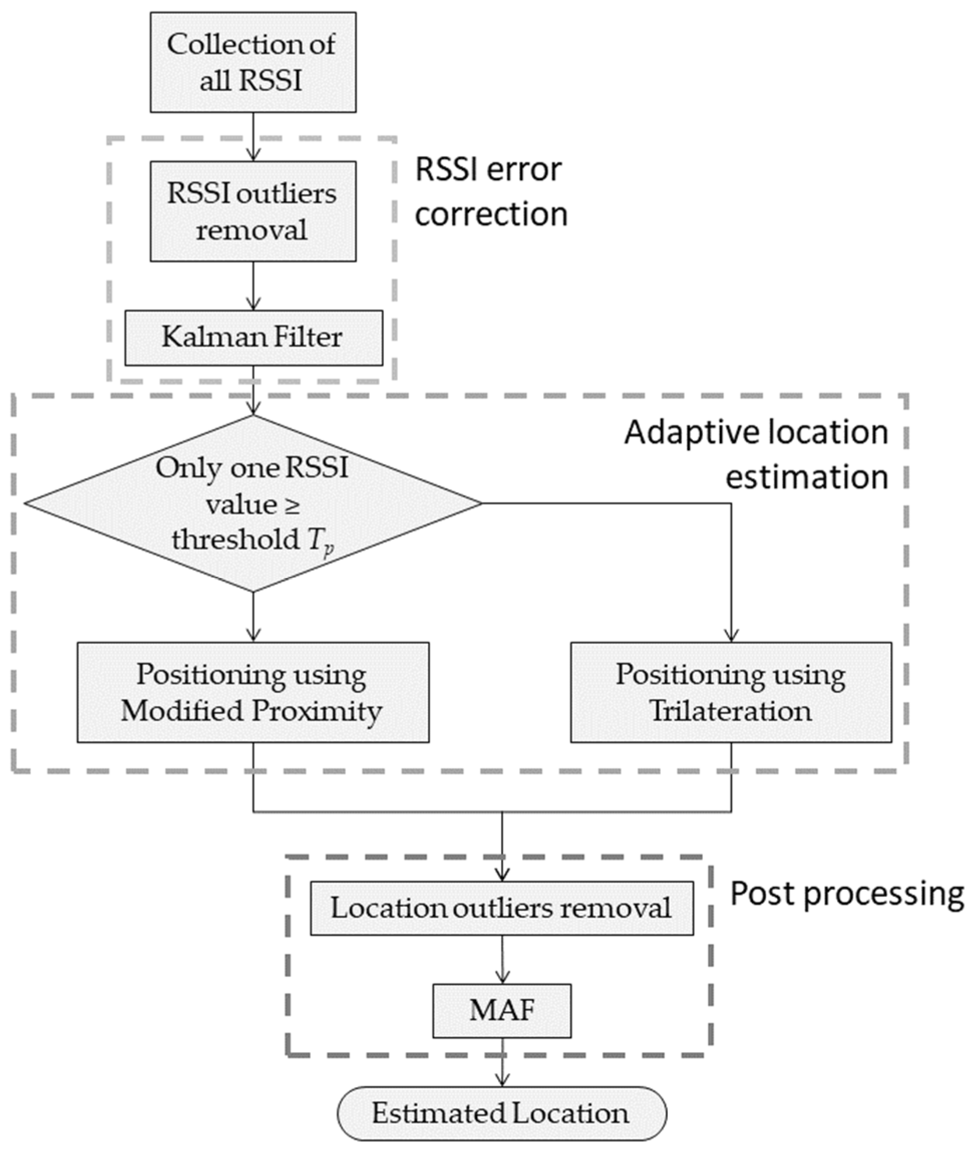
3. Proposed Indoor Positioning Method

In this paper, we propose the PAP algorithm for RSSI-based indoor positioning. The proposed method is structured into three steps: RSSI error correction, adaptive location estimation, and post-processing. The RSSI error correction step removes outliers and corrects noise in collected RSSIs. The adaptive location estimation step selects either a conventional trilateration or MP technique based on distances from APs for a positioning method. The position is determined through only one AP if an RSSI received from this AP is higher than a certain threshold T_p. Location outliers are removed in the post-processing step by excluding estimated coordinates outside designated positioning regions. Then, positioning results are corrected by the moving average filter, which collects the estimated coordinates and obtains the average coordinates in a window. Figure 1 illustrates the flow for the proposed method.

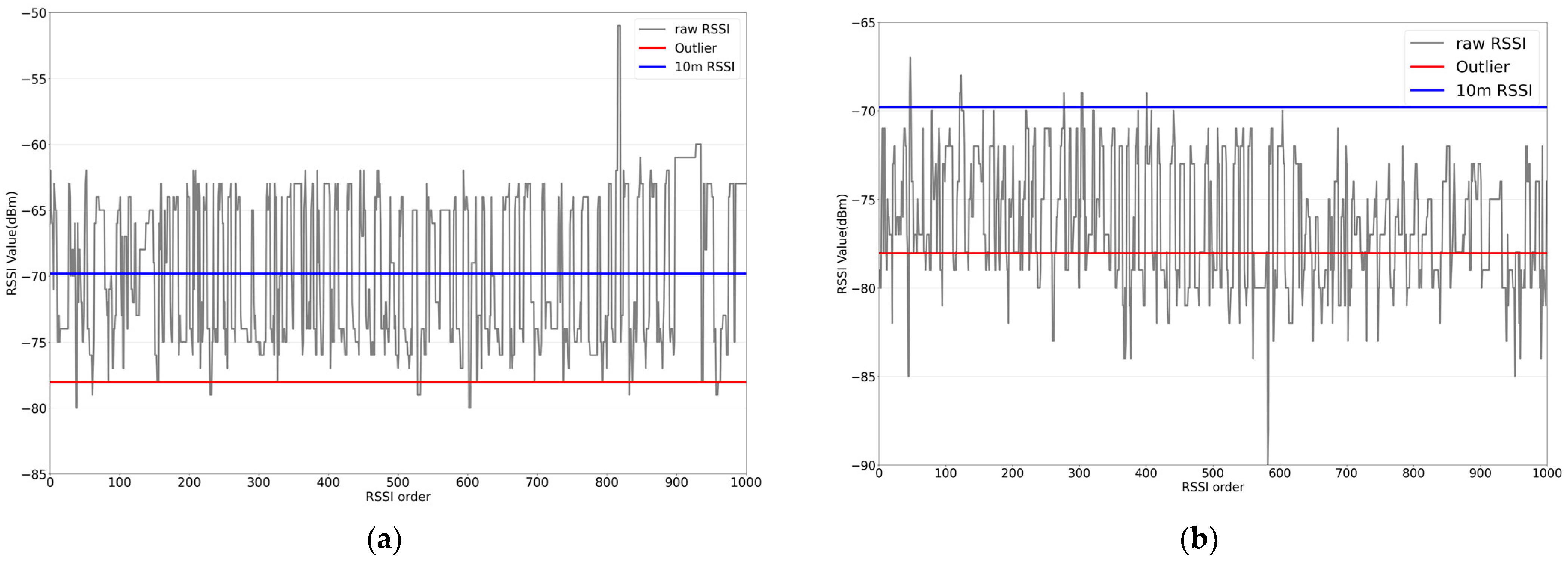
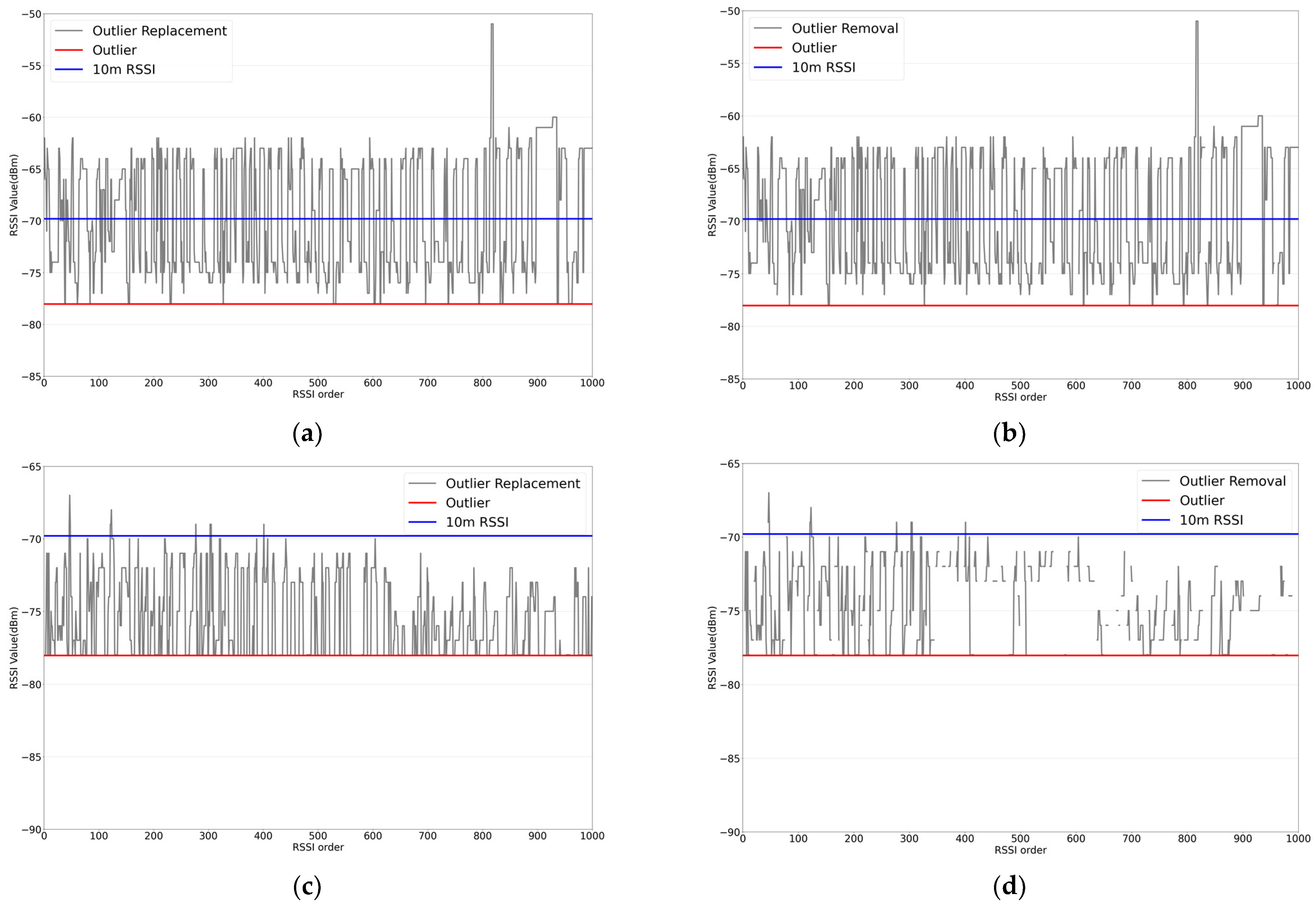
3.1. RSSI Error Correction

RSSI is an indicator representing the strength of a received signal. The optimal parameters of a radio propagation model, which describes relations between distance and RSSI, depend on the environment between an AP and a receiver. For indoor environments, LDPLM is widely adopted as the radio propagation model [21,22,23,24]. LDPLM calculates a distance from an AP to an RSSI as follows:

$$PL=P{L}_0+10n{\log }_{10}\left(\frac{d}{d_0}\right)$$

(1)

where d represents the distances between both the AP and receiver, d₀ is a predefined reference distance, PL and PL₀ are RSSIs measured at distances d and d₀, respectively, and n is a path loss exponent. The path loss exponent n is determined based on the spatial environment of a measurement space. Typically, n is known to be optimal in the range of 2–3 for a space without any obstacles and 4–6 for a space with many obstacles [21]. Equation (1) is rearranged for d as follows:

$$d={10}^{\frac{PL-P{L}_0}{10n}}{d}_0$$

(2)

RSSI outliners may be received due to phenomena such as refraction and reflection caused by obstacles on propagation paths. To remove these outliers, a threshold T_o is set as follows:

$$T_o=-10n{\log }_{10}\left(d_{max}\right)+\alpha$$

(3)

where d_max is the maximum reception distance within the positioning region and α is a reference RSSI value at a distance of 1 m.

RSSI measurements may vary depending on the presence of obstacles along the signal receiving path. Environments with and without obstacles along the straight path between the transmitter and receiver are referred to as LOS (line of sight) and NLOS (non-line of sight), respectively. Noise in the RSSIs is greater in LOS than in NLOS. Figure 2 shows RSSI measurements 1000 times at a distance of 10 m in both LOS and NLOS. In Figure 2, RSSI data are collected by a beacon with iBeacon protocol, a transmission power of 5 dBm, and an advertising interval of 100 ms. Additionally, the smartphone receiver is a Samsung Galaxy S22, equipped with Bluetooth version 5.2. Black, red, and blue solid lines in Figure 2 represent the measured RSSI values, the threshold (T_o) for outliers, and an RSSI corresponding to a distance of 10 m, respectively. RSSIs are measured in a range from −80 to −50 in LOS and from −90 to 65 in NLOS, respectively. Despite measuring signals at the same distance, lower RSSIs are generally measured in the NLOS environment compared to the LOS environment. Furthermore, the RSSI collected from NLOS contains many outliers that cannot be measured in a positioning environment.

RSSI outliers can be handled through outlier removal or replacement. For RSSI outlier removal or replacement, RSSIs that are lower than T_o are removed or replaced with T_o. Figure 3 and

Table 2. RSSI MAEs for different outlier handling methods.

	RSSI MAE
	No Handling	Outlier Removal	Outlier Replacement
LOS	2.55	2.48	2.53
NLOS	4.01	2.69	3.46

show the corrected and actual distances through outlier removal and replacement and their MAEs (mean absolute errors) with respect to Figure 2, respectively. Both outlier removal and replacement have similar MAEs in LOS because outliers occur infrequently. For the RSSI MAEs in NLOS, outlier removal is better than outlier replacement. It is difficult to handle RSSI outliers through outlier replacement, although outliers are replaced with a certain normal value. Therefore, OR (outlier removal) is adopted as an outlier handling method for unstable RSSI.

After handling the RSSI outliers, KF is applied to correct highly fluctuating RSSIs caused by noise [32,33]. KFs adjust current RSSIs through RSSIs predicted using previous RSSIs with measured RSSIs as follows:

$$s_t=s_t^{\prime }+K_t\left(m_t-s_t^{\prime }\right)$$

(4)

where $s_t$ is the predicted RSSI, $s_t^{\prime }$ is the predicted RSSI, m_t is the measured RSSI, and K_t is a Kalman gain that is weighted to the predicted and measured RSSIs. K_t is calculated as follows:

$$K_t=P_t^{\prime }{\left(P_t^{\prime }+R\right)}^{-1}$$

(5)

where R and $P_t^{\prime }$ are a measurement noise and an error covariance, respectively. R represents the reliability of the measurement. The measurement becomes more negligible as R increases. Typically, the optimal value for R is determined experimentally. The initial error covariance $P_0^{\prime }$ is set to 1. Then, the error covariance is updated as follows:

$$P_{t+1}^{\prime }=P_t+Q$$

(6)

where Q represents a process noise and P_t is a calculated covariance as follows:

$$P_t=\left(1-K_t\right)P_t^{\prime }$$

(7)

Figure 4 shows the RSSI correction through the KF. The gray, blue, and red solid lines represent the raw RSSIs, the corrected RSSIs through KF, and an RSSI at a distance of 5 m, respectively. The KF reduces distance estimation errors by smoothing the RSSIs.

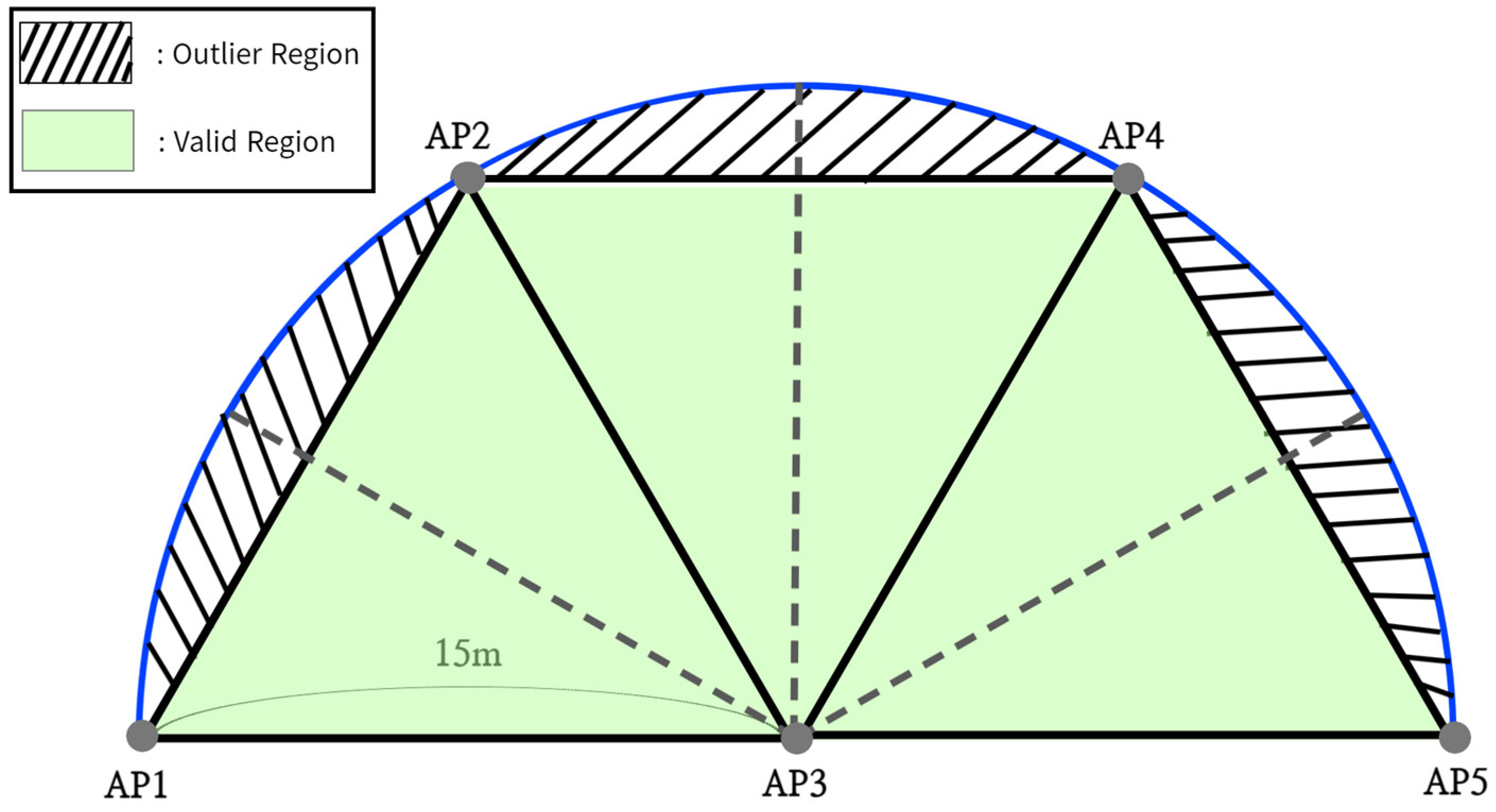
3.2. Adaptive Location Estimation

For a general state which is not in proximity to any AP, the trilateration technique [14,15] is employed for position estimation. Conversely, the proposed algorithm adopts the MP technique for position estimation if the receiver has a large proximity to a specific AP.

The trilateration technique involves estimating the position using the straight-line distances from three points. Indoor positioning using the trilateration technique converts the RSSI collected from three APs into distances and can thereby estimate the location of the receiver. Figure 5 shows the determination of a receiver location through three AP distances. Three circles in Figure 5 are formed with the distance as the radius based on the locations of AP1, AP2, and AP3 and the distance from each AP to the receiver. The receiver location is determined as a point where the three circles commonly intersect.

The distance r_i between ith AP and the receiver is calculated as follows:

$$\begin{array}{c}{r}_1^2={(x-x_1)}^2+{(y-y_1)}^2\\ r_2^2={(x-x_2)}^2+{(y-y_2)}^2\\ r_3^2={(x-x_3)}^2+{(y-y_3)}^2\end{array}$$

(8)

where (x, y) represents the coordinates of the receiver, and (x_i, y_i) (i = 1, 2, 3) are the coordinates of ith AP. The coordinates of the receiver are calculated by rearranging Equation (8) with x and y as follows:

$$\begin{array}{c}x=\frac{\left(r_2^2-r_3^2-x_2^2+x_3^2-y_2^2+y_3^2\right)\left(y_2-y_1\right)-\left(y_3-y_2\right)\left(r_1^2-r_2^2-x_1^2+x_2^2-y_1^2+y_2^2\right)}{2\left(\left(y_2-y_1\right)\left(x_3-x_2\right)-\left(y_3-y_2\right)\left(x_2-x_1\right)\right)}\\ y=\frac{\left(r_2^2-r_3^2-x_2^2+x_3^2-y_2^2+y_3^2\right)\left(x_2-x_1\right)-\left(x_3-x_2\right)\left(r_1^2-r_2^2-x_1^2+x_2^2-y_1^2+y_2^2\right)}{2\left(\left(x_2-x_1\right)\left(y_3-y_2\right)-\left(x_3-x_2\right)\left(y_2-y_1\right)\right)}\end{array}$$

(9)

A previous approach for positioning [34] primarily identifies which AP is closest to the receiver to estimate the approximate region. However, this technique has proven difficult for indoor localization due to significant errors in the physical location of the actual receiver. Although this problem can be alleviated by increasing the number of AP installations to refine the region and identify the locations, it is not an efficient positioning technique because the cost increases in proportion to the number of APs. The proposed MP technique can solve the limitations of the previous proximity technique. Since the MP technique is selectively applied only in cases of extremely close proximity to a specific AP, it does not need additional AP installations in other regions. Unlike the existing proximity technique, the MP technique considers the distance to the identified nearby AP based on the received RSSI and the AP locations. Therefore, the MP technique is a more accurate positioning method compared to the conventional proximity technique. The MP technique internally varies its positioning technique depending on the identified locations of nearby APs. Virtual numbers are sequentially mapped to the installed APs, as shown in Figure 6. If the AP number is not first or last, the AP location is estimated by vertically moving the position a distance r from the nearby AP to the inner region, as shown in Figure 7. The method of position estimation through vertical shifting differs based on whether the identified AP number is odd or even. If the number identified as a nearby AP is odd, such as AP3 in Figure 7, the distance calculated by calculating the RSSI collected from the nearby AP is defined as r. Afterward, the coordinates obtained by adding the distance r to the y-coordinate of the identified nearby AP location coordinates are taken as the location estimation result. If the identified nearby AP number is even, the AP location is estimated by subtracting distance r from the y-coordinate of the respective AP’s location coordinates.

When the AP has the first or last number, the same estimation method cannot be applied. The estimated location will be outside the intended region if the AP location is determined vertically. The position is determined for the AP with the first or last number by moving a distance of r toward the incenter of an equilateral triangle formed by three neighboring APs, including the identified nearby AP. The position moved a distance r towards the incenter from an identified nearby AP can be calculated by the trigonometric ratio and the properties of triangles that the incenter of a triangle is the intersection point of its angle bisectors. As shown in Figure 8, a line toward the incenter can be formed by drawing an angle bisector of length r from AP1. Additionally, we can obtain a virtual right triangle with this bisector as the hypotenuse. With the knowledge of all angles and the hypotenuse length of this right-angled triangle, the x- and y-coordinates of the estimated position can be calculated using trigonometric ratios. For the imaginary right triangle, cos 30° for the AP1 vertex is equal to the x-coordinate to be estimated divided by the hypotenuse length r. This expression is then rearranged to formulate the x-coordinate, resulting in the computation of x as r·cos 30°. For the imaginary right-angled triangle, where the vertex representing the estimated position has an angle of 60°, the cos 60° at this vertex is equivalent to the y-coordinate divided by the hypotenuse length r. This relationship can be rearranged to derive a formula for the y-coordinate, resulting in the calculation of y as r·cos 60°. Conversely, if the identified AP is the last number, x is subtracted from r·cos 30° and y is subtracted from r·cos 60° using the coordinates of the last AP location, and the coordinates are used as the estimated location.

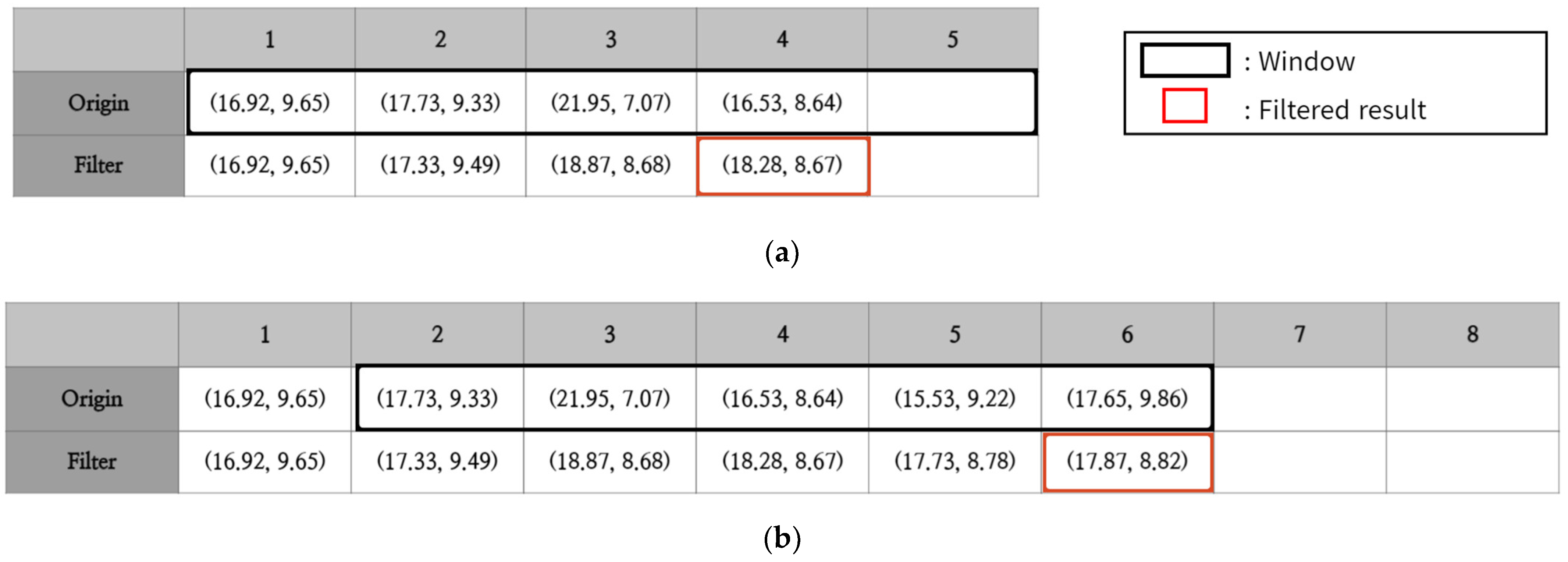
3.3. Post-Processing

The post-processing step involves a LOR (location outlier removal) and is conducted using a moving average filter (MAF).

The estimated location coordinates must exist only in the valid region formed by the APs and must not exist outside the valid region, such as outside of a building, on a wall, or in an impassable region. The possible valid region for positioning is inside the triangle where the AP is installed, as shown in the green region of Figure 9. A blue arc in Figure 9 means a maximum reception distance from AP3 after applying OR. Although the inaccuracy of trilateration positioning is reduced by removing RSSI outliers in the OR step, there is still the possibility of positioning outside the valid region, as shown in the hatched region of Figure 9. To prevent positioning outside of this valid region, LOR is applied. LOR removes the estimated location coordinate if it is outside the valid region.

Despite correcting the unstable one-dimensional RSSI through the RSSI filtering process, there are still instabilities when calculating two-dimensional coordinates through the mathematical operations of trilateration. To enhance positioning accuracy and improve precision, filtering for the two-dimensional coordinates is necessary. The MAF is commonly adopted to improve precision when noise exists in the data for tracking moving objects [35]. MAF calculates the average of the collected data within a fixed window size. Since the MAF operates using a sliding window approach, where the window moves one step at a time, it can calculate positioning results from collected signals without any loss in quantity. Figure 10 illustrates the MAF process. In Figure 10a, during the initial step where fewer data points are collected than the window size, the positioning results are obtained by averaging the collected coordinates. Subsequently, in a sliding window structure as shown in Figure 10b, the coordinates are averaged over the window size to determine the positioning results, and this process repeats. In this paper, the window size is set to 5. Utilizing MAF allows for the correction of abrupt changes in estimated positions, thereby enhancing both the accuracy and precision of the positioning results.

4. Experimental Results

In this paper, we used FSC-BP101E as the APs for the experiments. The receiver utilizes a Galaxy S22 smartphone based on the Android operating system.

4.1. Determining the Optimal Parameters of the Log-Distance Path Loss Model

For the proposed method, experiments are conducted to select the optimal parameters PL₀ and n for the LDPLM representing the relation between the RSSI and distance. To determine PL₀, the distance between the beacon and the receiver is set to 1 m. We collected 1000 signals. The RSSI measurement unit is dBm and ranges from 0 to –100. The RSSI value is closer to 0 as the signal is stronger. Figure 11 shows the histogram of RSSI collected at a distance of 1 m. RSSI fluctuates irregularly between −18 dB and −42 dB. The PL₀ value is selected as −23 dB, which is the mode among the collected RSSI values.

To obtain the path loss exponent n, RSSI is collected at different distances of 3 m, 5 m, 10 m, and 15 m in LOS environments. Additionally, RSSI is collected at 10 m and 15 m distances in NLOS environments. A total of 1000 signals are collected for each distance. To determine the optimal n, we calculate n from 1000 data points collected at each distance and then compute the average. n can be calculated through Equation (1).

The total average of n for each distance is calculated. For this experiment, an optimal path loss exponent of 4.68 is chosen for the relationship between RSSI and distance.

Table 3. Distance-based path loss exponent average.

	3 m	5 m	10 m	15 m	10 m NLOS	15 m NLOS	Total
n Average	5.52	4.35	4.35	3.83	5.05	4.96	4.68

presents the average path loss exponent collected for each distance and the final selected path loss exponent. In this paper, the parameters for calculating the threshold in Equation (3) are set as follows: α = −23, n = 4.68, and d = 15.

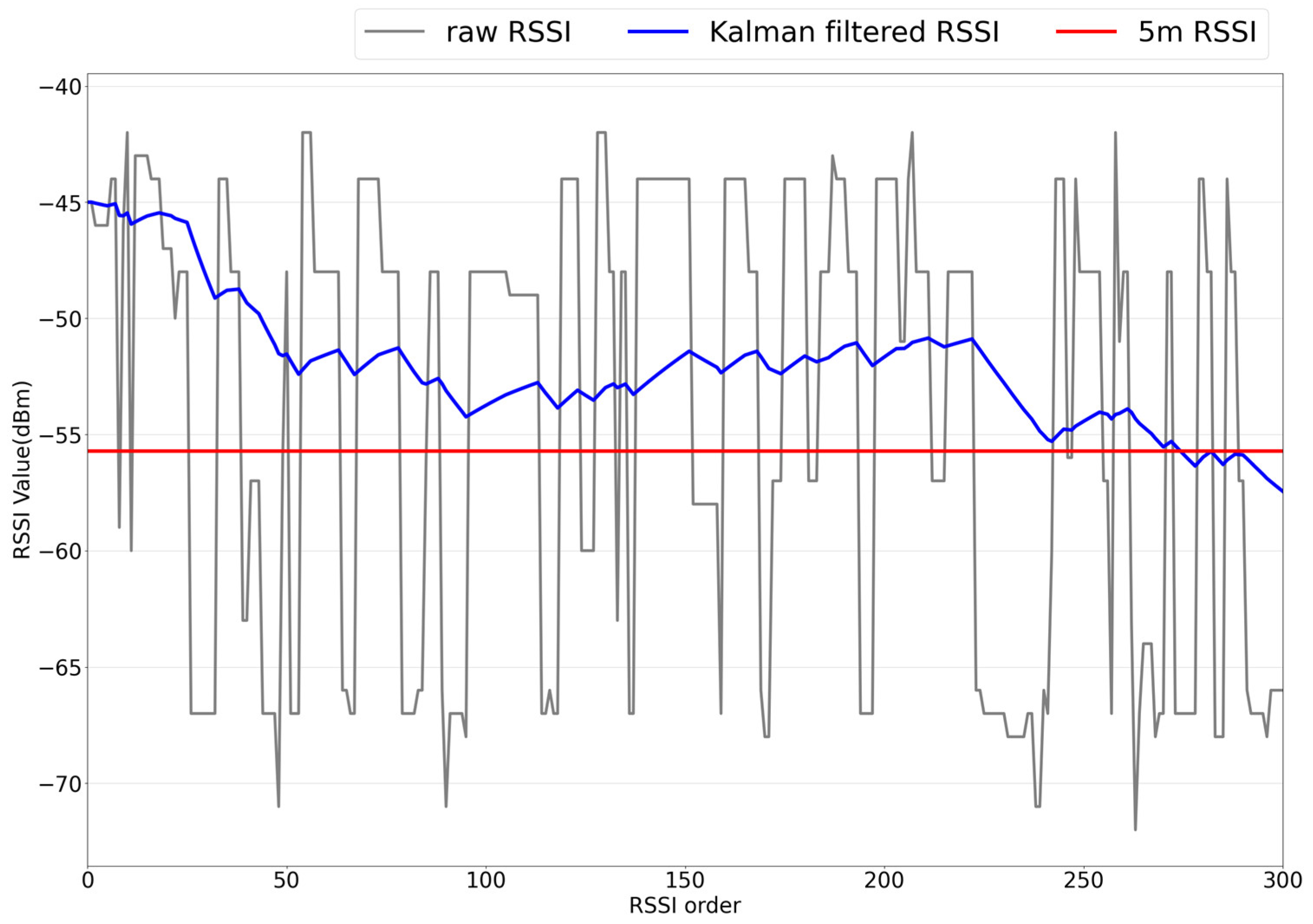
4.2. Determining the Optimal Parameters of a Kalman Filter

KF parameters, such as the process noise Q and measurement noise R, can be adjusted according to the environment. A value of 0.005 is applied for the Kalman parameter Q, and experiments are conducted to select R. The experiment collected 1000 signals in 1 m increments from 1 m to 15 m in LOS and NLOS environments. The sampling interval of the transmitter is set to 100 ms. To obtain the optimal R, we experimented with KF with R set to 1.25, 2.5, and 20. R is selected by comparing the distance MAE of the results of applying various KF configurations to each distance. Experimental results indicate that in both LOS and NLOS environments, the lowest distance estimation error is observed when R is set to 20, as shown in

Table 4. Distance MAE according to R.

Measurement Noise	Original	R = 20	R = 1.25 [24]	R = 2.5 [36]
LOS MAE	4.47	2.43	2.48	2.45
NLOS MAE	3.96	2.77	2.82	2.78

. Therefore, the KF parameter R is selected as 20.

4.3. Experiment with Proximity-Based Adaptive Algorithm

To measure the performance of the proposed method in real-world environments, experiments are conducted in an indoor environment with the layout shown in Figure 12. The thick lines in Figure 12 represent concrete walls with a thickness of approximately 0.2 m, while the gray dots indicate the positions of the beacons placed inside the building. Three adjacent beacons are installed to form an equilateral triangle with a side length of 15 m. There is a total of eight Beacons used for the experiment, covering an approximate region of 585 m². Figure 12 represents the positioned locations for accuracy measurement. In Figure 12, triangles indicate points proximate to the AP within 1 m, squares represent the center positions of three adjacent beacons, and stars denote arbitrarily designated points.

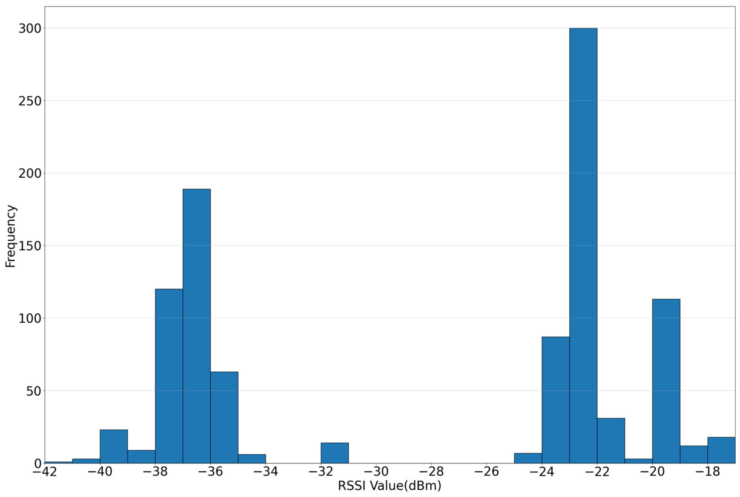
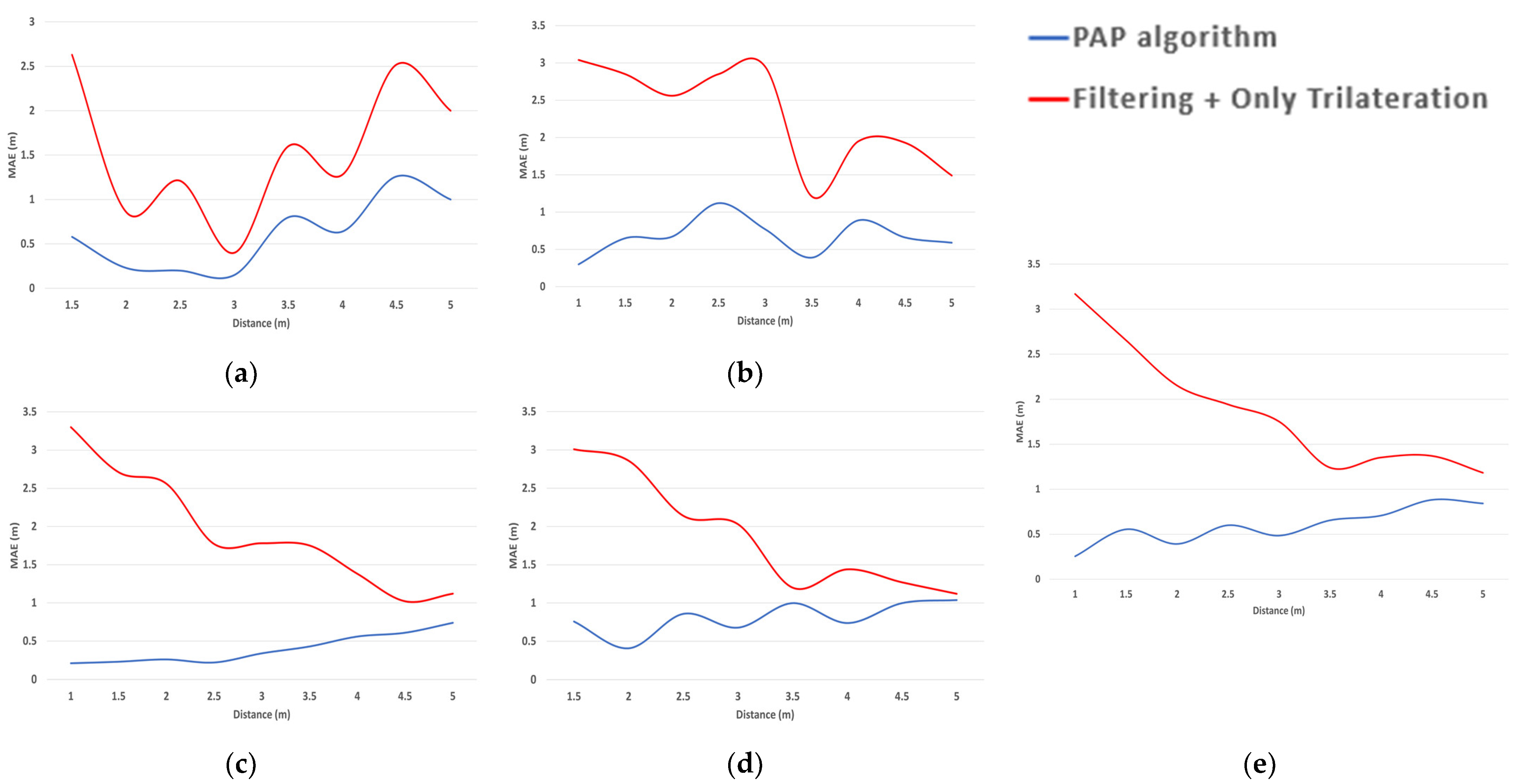
4.3.1. Proximity Threshold

For this session, experiments are conducted to determine the optimal threshold T_p, to identify situations where a device is sufficiently close to an AP in PAP algorithms. If T_p for the PAP algorithm is set to too large of a value, the RSSI value may be unstable and exceed T_p even if it is not close to the AP, so the MP technique is applied. This could lead to a degradation in the positioning accuracy of regions that are relatively stable in the existing positioning system, which solely relies on trilateration. Conversely, when T_p is set to an excessively low value, instances may occur where MP should be applied due to proximity to AP, but trilateration is performed due to failure to exceed T_p. This does not address the issues of position unavailability in weak-signal regions and degradation in positioning accuracy, which are inherent to trilateration-based positioning. Therefore, it is necessary to determine the optimal T_p for PAP algorithms through experimentation. T_p is set to 2 m, 3 m, 4 m, and 5 m, and 1000 localizations are conducted at each localization point.

Table 5. Distance MAE according to threshold T_p.

Threshold (m)	2.0	3.0	4.0	5.0
Side position	1.19	0.96	0.97	0.97
Center position	3.26	3.35	4.22	4.79
Other position	5.07	4.83	4.99	5.21
Average	3.17	3.05	3.39	3.66

evaluates the localization accuracy performance by calculating the error between the actual and localized positions at each localization point using the Euclidean distance and presents the localization accuracy according to the localization point type based on T_p.

For the case of 5 m, the largest T_p in the experiment, T_p is frequently exceeded at the center position and other position, resulting in increased errors when positioning is carried out using the MP technique. For the 2 m case, where T_p is the smallest, there are numerous instances where T_p is not surpassed at the side position, leading to the non-application of the MP technique and predominantly resorting to trilateration for positioning, consequently confirming an escalation in positioning errors. With a T_p of 3 m, positioning errors are found to be lower at the center position compared to the 2 m, yet the highest degree of positioning accuracy is observed at the side position and other position. Thus, with a T_p set at 3 m, it is validated that the PAP algorithm accurately identifies cases near an AP and enhances positioning accuracy through the utilization of the MP technique when in proximity. This paper adopts a T_p value of 3 m for positioning through the PAP algorithm.

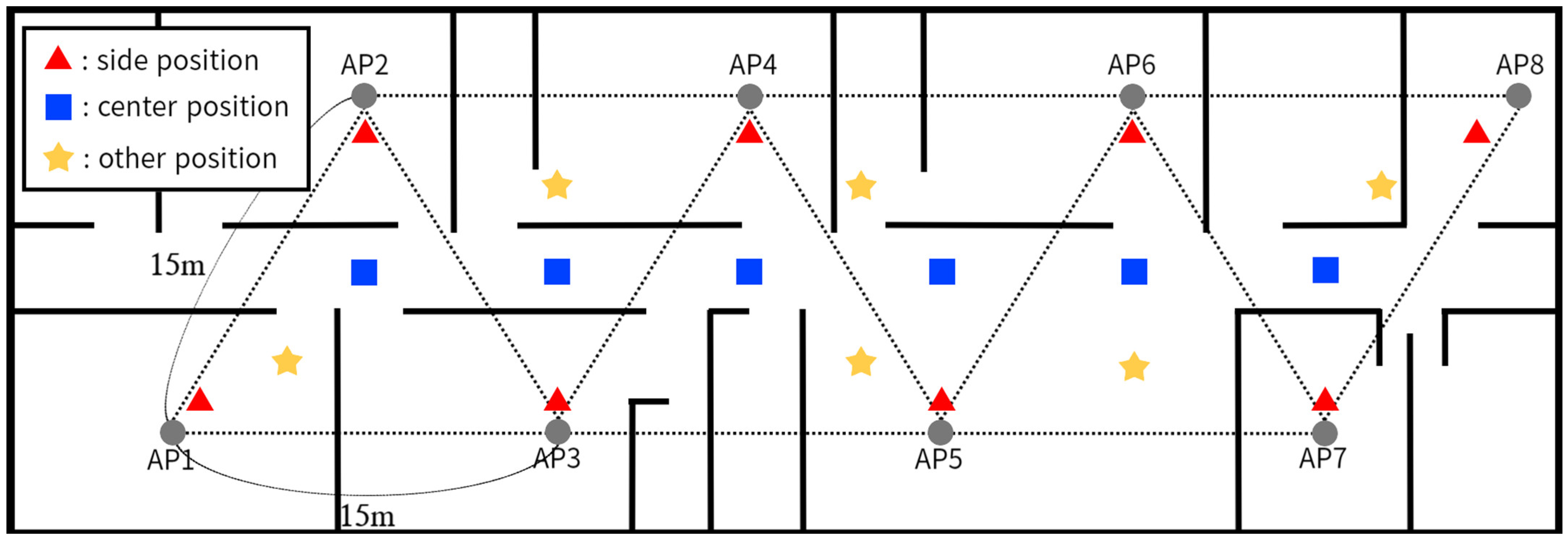
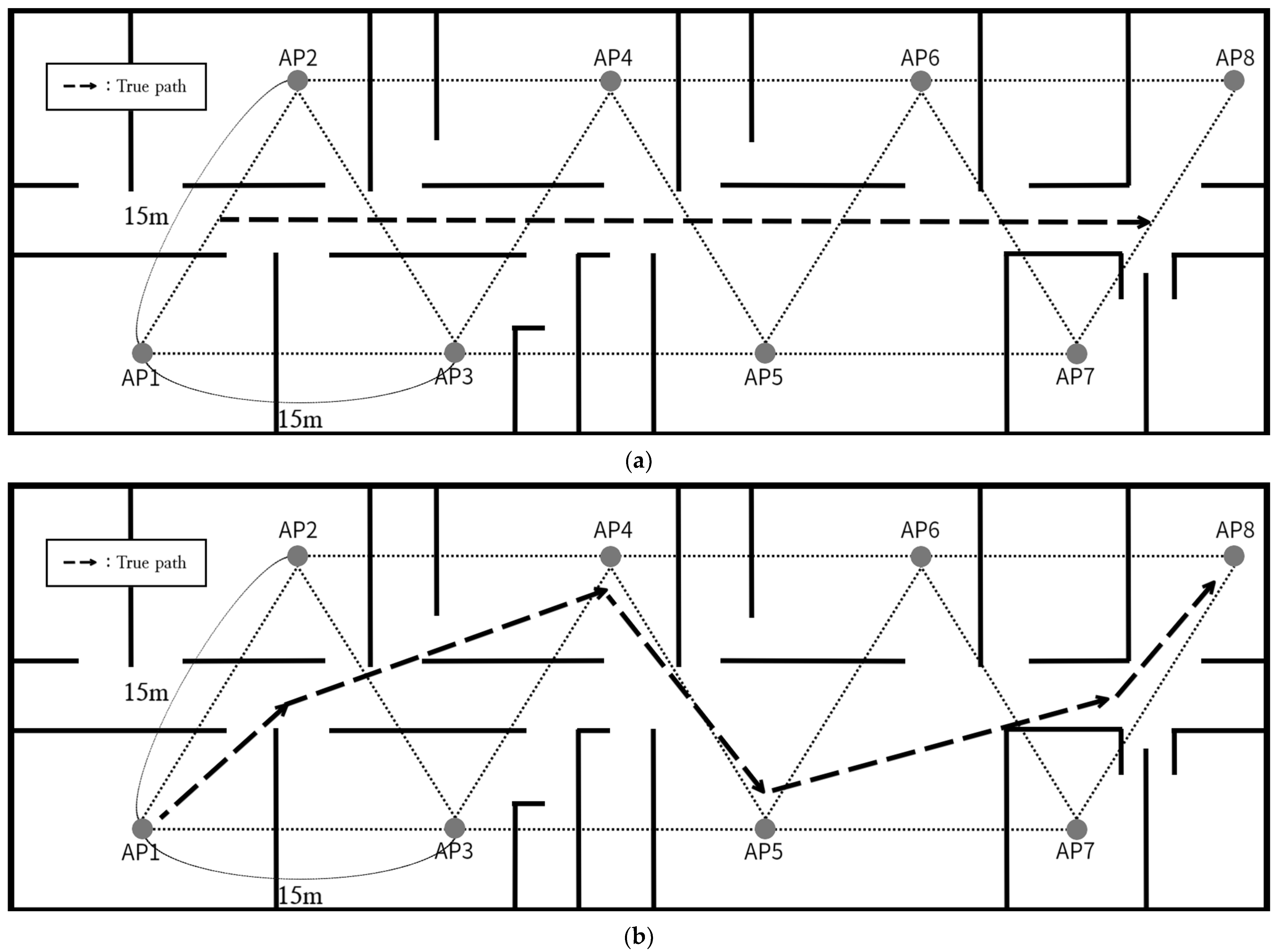
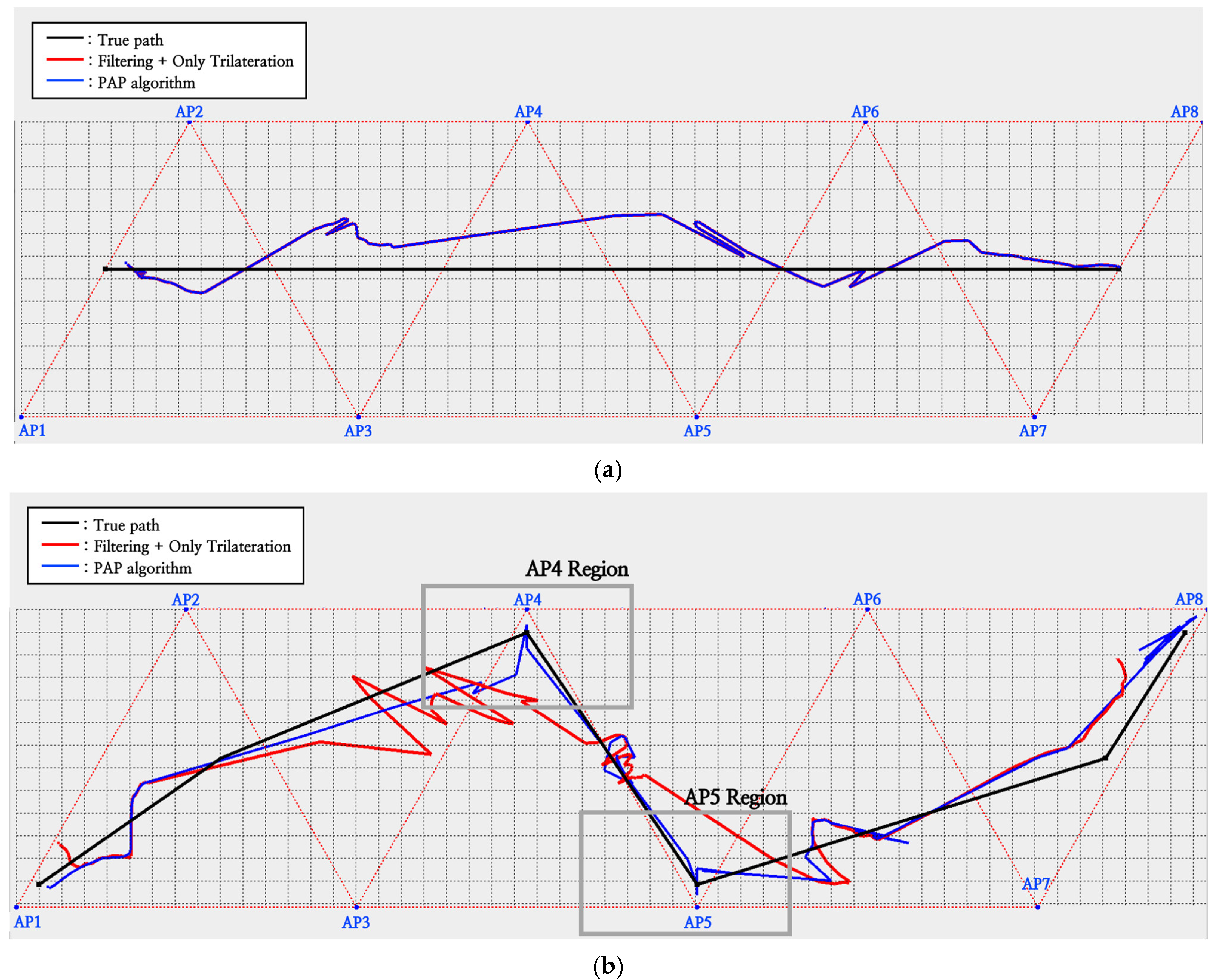
4.3.2. Experiment Evaluation in Static State

For this section, an experiment is conducted to assess and compare the efficacy of the proposed method under stationary conditions. The positioning points are shown in Figure 12. Positioning is iterated 1000 times at each of the 20 stationary points. For performance evaluation, we compare various filtering combinations. Three filtering combinations are considered: OR, OR + KF, and OR + KF + LOR + MAF. Each combination is tested with and without the application of the MP technique. The proposed method is the PAP algorithm, which means OR + KF + LOR + MAF filtering and location estimation using trilateration and MP techniques depends on proximity. The threshold T_p for identifying proximity status in the PAP algorithm is set at 3 m.

Table 6. Evaluation of experiment performance at static state.

	Method					Errors (m)
Trilateration	MP	OR	KF	LOR	MAF	Side Position	Center Position	Other Position	Average
O						3.88	3.81	4.74	4.14
O		O				3.01	3.30	4.35	3.55
O		O	O			3.02	2.72	4.45	3.40
O		O	O	O	O	2.73	2.70	4.44	3.29
O	O					0.98	4.11	4.36	3.15
O	O	O				0.96	3.60	4.34	2.97
O	O	O	O			0.89	2.72	3.90	2.50
O	O	O	O	O	O	0.75	2.70	3.68	2.38

presents the average Euclidean distance between the estimated and actual position coordinates as a result of performance comparison under stationary conditions, contingent upon the application of the filtering algorithm and MP. In Table 6, ‘O’ means that the corresponding technique or filtering is applied to the positioning method. Methods using the MP technique show overall improved performance compared to methods using only trilateration. In particular, the MP technique reduced positioning errors for side positions located within 1 m of the AP. Other positions also exhibited lower positioning errors when the MP technique was applied. For center positions, where occurrences of exceeding T_p, indicating proximity to the AP, are almost nonexistent, applying KF would result in the same outcome regardless of whether MP is applied. However, in methods where KF is not applied to RSSI, intermittent occurrences of exceeding T_p are observed due to the unstable RSSI being directly applied, prompting the application of MP. The static state experiment results are obtained by calculating 1000 consecutive position estimation coordinates for each method and the actual physical receiver position coordinates using the Euclidean distance formula, and the unit is meters (m). For the experimental results, the average positioning error of the method using raw RSSI and only the trilateration technique is about 4.14 m, and the average positioning error of the method using only the trilateration technique by applying OR + KF + LOR + MAF filtering is about 4.14 m. Since it is 3.29 m, the positioning accuracy is reduced by about 21%. In addition, the result of positioning using the PAP algorithm is that OR + KR + LOR + MAF filtering is applied, and trilateration and MP technique positioning are included. The average positioning error is about 2.38 m, so OR + KF + LOR + MAF filtering is applied, and the position error is reduced by about 28% compared to the positioning error determined using only trilateration.

4.3.3. Experiment Evaluation in Dynamic State

For this session, dynamic state experiments are conducted to validate the overall performance of the proposed PAP algorithm and the effectiveness of the MP technique. Figure 13 shows the positioning environment floor plan and the dashed lines representing the positioning movement paths for the dynamic state experiments. The total movement distance in Figure 13a is 45 m, while it is approximately 63 m in Figure 13b.

The dynamic positioning test evaluates the performance of the PAP algorithm by comparing the performance of the proposed method with a positioning technique using only trilateration with the same filtering algorithm applied. For the experiment, location estimation is conducted while moving at a constant speed along a designated path. Figure 14 shows the location estimation results of the experiment along the positioning path. In Figure 14, the black solid line is the actual path, the red solid line represents the location estimation path using only trilateration, and the blue solid line represents the location estimation path through the PAP algorithm. Figure 14a shows the experimental results when walking in a straight line through the middle of APs. Positioning in the central region is not close to the AP, so the MP technique is not applied. As a result, the solid red line and solid blue line show the same positioning results. In the case of the experimental results measured along the path in Figure 14b, differences can be seen with or without the MP technique applied. For the AP4 and AP5 regions, the solid blue line shows that when the path is close to the AP, the MP technique is applied, and the positioning is similar to the actual path. However, the solid red line did not reach the region close to the AP, and the positioning continued along the next movement route. This can be seen as a phenomenon that occurs due to the problem of positioning in trilateration in weak signal regions. When approaching an AP, the RSSI of one AP is strong, but the RSSI of the other two APs is weak due to the NLOS environment. Therefore, RSSI is deleted through OR, making positioning impossible at that location. Therefore, the red solid line represents the actual path and the location estimation result with a large error, especially when close to the AP. Figure 15 presents a graph of the position estimation error of the experimental results on the actual path within 5 m of AP1, AP4, AP5, and AP8 in Figure 14b. The solid red line shows the positioning error using trilateration only, and the solid blue line shows the error of the PAP algorithm. It is shown that the error in positioning using the PAP algorithm decreases significantly as it gets closer to the AP. This indicates that the PAP algorithm, where the MP technique is applied when close to the AP, helps improve positioning accuracy.

5. Conclusions

In this paper, a PAP algorithm is proposed to improve the accuracy of indoor positioning systems. The AP proximities were measured through the collected RSSIs to select the positioning technique in the adaptive location estimation step. If one RSSI was higher than the specific threshold, the position was estimated through one AP corresponding to this RSSI. Otherwise, conventional trilateration was applied. We removed the positioning results that cannot be actual positions and corrected them through MAF in the post-processing step. The PAP algorithm addresses the problem of the previous trilateration-based methods, which is unattainable positioning in signal-weak regions, without affecting accuracy in other regions. The static experiment results indicate that the positioning accuracy improves by approximately 21% and 28% in cases of applying the RSSI correction and MP techniques, respectively. The dynamic experiment shows an accuracy improvement of about 45% for the proposed algorithm compared to conventional trilateration. In future research, it is possible to consider a positioning technique through the integration of other technologies in regions where both trilateration and MP techniques exhibit vulnerabilities. First, with proximity identified, the location estimated using the MP technique can be set as the reference location. Dead-reckoning navigation techniques via IMU (inertial measurement unit) sensors can then be added for further tracking. Through this method, consistent positioning performance can be achieved at all measurement locations within the target region.

References

1. Zaim, D.; Bellafkih, M. Bluetooth Low Energy (BLE) based Geomarketing System. In Proceedings of the 2016 11th International Conference on Intelligent Systems: Theories and Applications (SITA), Mohammedia, Morocco, 19–20 October 2016; pp. 1–6. [Google Scholar]
2. Guerreiro, J.A.; Ahmetovic, D.; Sato, D.; Kitani, K.; Asakawa, C. Airport Accessibility and Navigation Assistance for People with Visual Impairments. In Proceedings of the CHI Conference on Human Factors in Computing Systems, Glasgow, UK, 4–9 May 2019; pp. 1–14. [Google Scholar]
3. Hwangbo, H.; Kim, J.; Lee, Z.; Kim, S. Store layout optimization using indoor positioning system. Int. J. Distrib. Sens. Netw. 2017, 1, 155014771769258. [Google Scholar] [CrossRef]
4. Fadzilla, M.A.; Harun, A.; Shahriman, A.B. Localization Assessment for Asset Tracking Deployment by Comparing an Indoor Localization System with a Possible Outdoor Localization System. In Proceedings of the 2018 International Conference on Computational Approach in Smart Systems Design and Applications (ICASSDA), Kuching, Malaysia, 15–17 August 2018; pp. 1–6. [Google Scholar] [CrossRef]
5. Yang, Y.; Ding, Y.; Yuan, D.; Wang, G.; Xie, X.; Liu, Y.; He, T.; Zhang, D. Transloc: Transparent Indoor Localization with Uncertain Human Participation for Instant Delivery. In Proceedings of the 26th Annual International Conference on Mobile Computing and Networking (MobiCom ‘20), New York, NY, USA, 21–25 September 2020; pp. 1–14. [Google Scholar] [CrossRef]
6. Gikas, V.; Dimitratos, A.; Perakis, H.; Retscher, G.; Ettlinger, A. Full-Scale Testing and Performance Evaluation of an Active RFID System for Positioning and Personal Mobility. In Proceedings of the 2016 International Conference on Indoor Positioning and Indoor Navigation (IPIN), Alcala de Henares, Spain, 4–6 October 2016; pp. 1–8. [Google Scholar] [CrossRef]
7. Basiri, A.; Lohan, E.S.; Moore, T.; Winstanley, A.; Peltola, P.; Hill, C.; Amirian, P.; Figueiredo e Silva, P. Indoor location based services challenges requirements and usability of current solutions. Comput. Sci. Rev. 2017, 24, 1–12. [Google Scholar] [CrossRef]
8. Chen, Z.; Zou, H.; Jiang, H.; Zhu, Q.; Soh, Y.C.; Xie, L. Fusion of wifi, smartphone sensors and landmarks using the kalman filter for indoor localization. Sensors 2015, 15, 715–732. [Google Scholar] [CrossRef] [PubMed]
9. Guo, W.; Jing, L. Toward low-cost passive motion tracking with one pair of commodity Wi-Fi devices. IEEE J. Indoor Seamless Position. Navig. 2023, 1, 39–52. [Google Scholar] [CrossRef]
10. Lee, N.; Ahn, S.; Han, D. AMID: Accurate magnetic indoor localization using deep learning. Sensors 2018, 18, 1598. [Google Scholar] [CrossRef] [PubMed]
11. Yassin, A.; Nasser, Y.; Awad, M.; Al-Dubai, A.; Liu, R.; Yuen, C.; Raulefs, R.; Aboutanios, E. Recent Advances in Indoor Localization: A Survey on Theoretical Approaches and Applications. IEEE Commun. Surv. Tutor. 2017, 19, 1327–1346. [Google Scholar] [CrossRef]
12. Dong, J.; Lian, Z.; Xu, J.; Yue, Z. UWB localization based on improved robust adaptive cubature Kalman Filter. Sensors 2023, 23, 2669. [Google Scholar] [CrossRef] [PubMed]
13. Daniş, F.S. Practical and parameterized fingerprinting through maximal filtering for indoor positioning. IEEE J. Indoor Seamless Position. Navig. 2023, 1, 199–210. [Google Scholar] [CrossRef]
14. Noertjahyana, A.; Wijayanto, I.A.; Andjarwirawan, J. Development of Mobile Indoor Positioning System Application Using Android and Bluetooth Low Energy with Trilateration Method. In Proceedings of the 2017 International Conference on Soft Computing, Intelligent System and Information Technology (ICSIIT), Denpasar, Indonesia, 26–29 September 2017. [Google Scholar] [CrossRef]
15. Bai, L.; Ciravegna, F.; Bond, R.; Mulvenna, M. A low cost indoor positioning system using bluetooth low energy. IEEE Access 2020, 8, 136858–136871. [Google Scholar] [CrossRef]
16. Prasad, K.N.R.S.V.; Hossain, E.; Bhargava, V.K. Machine Learning Methods for RSS-Based User Positioning in Distributed Massive MIMO. IEEE Trans. Wirel. Commun. 2018, 17, 8402–8417. [Google Scholar] [CrossRef]
17. Führling, N.; Rou, H.S.; de Abreu, G.T.F.; González, G.D.; Gonsa, O. Robust received signal strength indicator (RSSI)-based multitarget localization via gaussian process regression. IEEE J. Indoor Seamless Position. Navig. 2023, 1, 104–114. [Google Scholar] [CrossRef]
18. Belmonte-Hernández, A.; Hernández-Peñaloza, G.; Martín Gutiérrez, D.; Álvarez, F. SWiBluX: Multi-sensor deep learning fingerprint for precise real-time indoor tracking. IEEE Sens. J. 2019, 19, 3473–3486. [Google Scholar] [CrossRef]
19. Gufran, D.; Tiku, S.; Pasricha, S. STELLAR: Siamese multiheaded attention neural networks for overcoming temporal variations and device heterogeneity with indoor localization. IEEE J. Indoor Seamless Position. Navig. 2023, 1, 115–129. [Google Scholar] [CrossRef]
20. Shang, S.; Wang, L. Overview of WiFi Fingerprinting-Based Indoor Positioning. IET Commun. 2022, 16, 725–733. [Google Scholar] [CrossRef]
21. Röbesaat, J.; Zhang, P.; Abdelaal, M.; Theel, O. An improved BLE indoor localization with Kalman-based fusion: An experimental study. Sensors 2017, 17, 951. [Google Scholar] [CrossRef] [PubMed]
22. Mackey, A.; Spachos, P.; Song, L.; Plataniotis, K.N. Improving BLE beacon proximity estimation accuracy through Bayesian filtering. IEEE IoT J. 2020, 7, 3160–3169. [Google Scholar] [CrossRef]
23. Milano, F.; da Rocha, H.; Laracca, M.; Ferrigno, L.; Espírito Santo, A.; Salvado, J.; Paciello, V. BLE-based indoor localization: Analysis of some solutions for performance improvement. Sensors 2024, 24, 376. [Google Scholar] [CrossRef]
24. Viswanathan, M.; Srinivasan, V. Wireless Communication Systems in Matlab, 2nd ed.; Independently Published: Chicago, IL, USA, 2020. [Google Scholar]
25. Liu, Y.; Li, N.; Wang, D.; Guan, T.; Wang, W.; Li, J.; Li, N. Optimization Algorithm of RSSI Transmission Model for Distance Error Correction. In Proceedings of the Advances in Intelligent Information Hiding and Multimedia Signal Processing, Jilin, China, 18–20 July 2020; Springer: Singapore, 2020. [Google Scholar] [CrossRef]
26. Yang, J.; Deng, S.; Lin, M.; Xu, L. An adaptive calibration algorithm based on RSSI and LDPLM for indoor ranging and positioning. Sensors 2022, 22, 5689. [Google Scholar] [CrossRef] [PubMed]
27. Fu, Y.; Chen, P.; Yang, S.; Tang, J. An indoor localization algorithm based on continuous feature scaling and outlier deleting. IEEE IoT J. 2018, 5, 1108–1115. [Google Scholar] [CrossRef]
28. Ozer, A.; John, E. Improving the Accuracy of Bluetooth Low Energy Indoor Positioning System Using Kalman Filtering. In Proceedings of the 2016 International Conference on Computational Science and Computational Intelligence (CSCI), Las Vegas, NV, USA, 15–17 December 2016. [Google Scholar] [CrossRef]
29. Jianyong, Z.; Haiyong, L.; Zili, C.; Zhaohui, L. RSSI Based Bluetooth Low Energy Indoor Positioning. In Proceedings of the 2014 International Conference on Indoor Positioning and Indoor Navigation (IPIN), Busan, Republic of Korea, 27–30 October 2014. [Google Scholar] [CrossRef]
30. Albraheem, L.; Alawad, S. A hybrid indoor positioning system based on visible light communication and bluetooth RSS trilateration. Sensors 2023, 23, 7199. [Google Scholar] [CrossRef]
31. Shiraki, S.; Shioda, S. Contact information-based indoor pedestrian localization using bluetooth low energy beacons. IEEE Access 2022, 10, 119863–119874. [Google Scholar] [CrossRef]
32. Shen, Y.; Hwang, B.; Jeong, J.P. Particle filtering-based indoor positioning system for beacon tag tracking. IEEE Access 2020, 8, 226445–226460. [Google Scholar] [CrossRef]
33. Kim, Y.; Bang, H. Introduction to Kalman Filter and Its Applications; IntechOpen: Rijeka, Croatia, 2019. [Google Scholar] [CrossRef]
34. Brida, P.; Matula, M.; Duha, J. Using Proximity Technolongy for Localization in Wireless Sensor Networks. Commun Sci. Lett. Univ. Zilina 2007, 9, 50–54. [Google Scholar] [CrossRef]
35. Sadowski, S.; Spachos, P. Optimization of BLE Beacon Density for RSSI-Based Indoor Localiztion. In Proceedings of the 2019 IEEE International Conference on Communications Workshops (ICC Workshops), Shanghai, China, 20–24 May 2019. [Google Scholar] [CrossRef]
36. Mackey, A.; Spachos, P. Performance Evaluation of Beacons for Indoor Localization in Smart Buildings. In Proceedings of the 2017 IEEE Global Conference on Signal and Information Processing (GlobalSIP), Montreal, QC, Canada, 14–16 November 2017. [Google Scholar] [CrossRef]
Figure 1. Flowchart for the proposed method.
Applsci 14 03319 g001
Figure 2. Signal effect depending on the presence or absence of obstacles at a distance of 10 m: (a) 10 m LOS raw RSSI; (b) 10 m NLOS raw RSSI.
Applsci 14 03319 g002
Figure 3. RSSI outlier handling: (a) outlier replacement in LOS; (b) outlier removal in LOS; (c) outlier replacement in NLOS; (d) outlier removal in NLOS.
Applsci 14 03319 g003
Figure 4. RSSI correction through Kalman filter.
Applsci 14 03319 g004
Figure 5. Trilateration example.
Applsci 14 03319 g005
Figure 6. An environment example of modified proximity positioning.
Applsci 14 03319 g006
Figure 7. An example of modified proximity positioning in the vicinity of AP3.
Applsci 14 03319 g007
Figure 8. An example of modified proximity positioning in the vicinity of AP1.
Applsci 14 03319 g008
Figure 9. An example illustrating outlier and valid regions.
Applsci 14 03319 g009
Figure 10. MAF example: (a) Initial state when data is collected below the window size; (b) General operating state.
Applsci 14 03319 g010
Figure 11. RSSI histogram at 1 m.
Applsci 14 03319 g011
Figure 12. Experimental environment.
Applsci 14 03319 g012
Figure 13. Localization paths: (a) straight path; (b) moving path.
Applsci 14 03319 g013
Figure 14. Experimental results by path type: (a) for straight path; (b) for moving path.
Applsci 14 03319 g014
Figure 15. Positioning error according to distance from AP: (a) AP1; (b) AP4; (c) AP5; (d) AP8; (e) average.
Applsci 14 03319 g015