Research on X-ray Diagnosis Model of Musculoskeletal Diseases Based on Deep Learning

Abstract

Musculoskeletal diseases affect over 100 million people globally and are a leading cause of severe, prolonged pain, and disability. Recognized as a clinical emergency, prompt and accurate diagnosis of musculoskeletal disorders is crucial, as delayed identification poses the risk of amputation for patients, and in severe cases, can result in life-threatening conditions such as bone cancer. In this paper, a hybrid model HRD (Human-Resnet50-Densenet121) based on deep learning and human participation is proposed to efficiently identify disease features by classifying X-ray images. Feasibility testing of the model was conducted using the MURA dataset, with metrics such as accuracy, recall rate, F1-score, ROC curve, Cohen’s kappa, and AUC values employed for evaluation. Experimental results indicate that, in terms of model accuracy, the hybrid model constructed through a combination strategy surpassed the accuracy of any individual model by more than 4%. The model achieved a peak accuracy of 88.81%, a maximum recall rate of 94%, and the highest F1-score value of 87%, all surpassing those of any single model. The hybrid model demonstrates excellent generalization performance and classification accuracy.

1. Introduction

Musculoskeletal (MSK) diseases encompass disorders affecting the muscles, bones, soft tissues, joints, and spine. Throughout the entire lifespan, from infancy to old age, MSK diseases may occur, exerting an impact on work productivity and economic output. Globally, the latest Global Burden of Disease (GBD) study estimates that 1.71 billion people worldwide suffer from MSK [1]. X-ray image diagnosis plays an important role in MSK diagnosis, and clinicians have many X-ray image reading tasks every day. At Beth Israel Deaconess Medical Center, it was reported that most radiology teachers and trainees worked more than eight hours in front of a personal computer or PACS monitor, and 58 percent experienced repetitive stress symptoms [2]. Similarly, in a survey by Thompson et al. showed that 60.2% of breast imaging radiologists reported repetitive stress symptoms [3]. Prolonged intensive work harms the accuracy and efficiency of medical practitioners in diagnosing musculoskeletal disorders. Errors in image interpretation leading to misdiagnosis or delayed correct diagnosis can cause significant harm to the patient’s body, and in extreme cases, pose a threat to their life.

In recent years, deep learning algorithms utilizing deep convolutional neural networks have undergone testing in medical imaging interpretation, achieving significant advancements [4]. Disease classification and diagnostic algorithms have been applied and validated in various medical imaging technologies including computed tomography (CT), magnetic resonance imaging (MRI), optical coherence tomography (OCT), and pathological images, among others [4]. Traditional machine learning algorithms for medical image recognition mainly involve two components: image feature extraction and image recognition. Human intervention is required for extracting features from medical images, leading to relatively low recognition accuracy [5,6]. Additionally, single models often fail to achieve the desired results in medical image recognition and classification, exhibiting weak adaptability and robustness. For instance, Shahedi et al. [7] achieved a segmentation of 83% Dice similarity coefficient for three-dimensional CT images of the prostate by using an improved U-Net network. Deep learning, as a data-driven approach, can automatically learn feature representations from a large volume of medical imaging data, thereby enhancing the diagnostic accuracy and efficiency. For instance, Jinbo Hu, Weizhi Nie, and others [8] proposed a deformable Transformer-assisted model for the diagnosis of chest X-ray image diseases, utilizing the extended ResNet50 as a feature extraction network. Multiple experiments were conducted on the ChestX-Ray14 and CheXpert datasets, achieving AUC values of 0.8398 and 0.9061, respectively. Yukun Chen, Zhuomin Zhang et al. [9] proposed a new AI-PLAX, based on two-stage photographs, that addressed the challenge of using photographs for the automated evaluation and examination of the placenta, which was capable of accurate morphological characterization and performed well in clinically meaningful feature analysis tasks. Lianzhong Jian et al. [10] introduced the ConvOS model for the diagnosis of COVID-19, utilizing the IGOS++ algorithm and an improved ConvNeXt network. The ConvOS model achieved an accuracy, recall rate, precision, and F1-score of 93.7%, 92.6%, 96.2%, and 94.4%, respectively.

In the field of medical imaging, medical image data present complex characteristics including noise, uncertainty, and class imbalance, which significantly impact physicians during pathological diagnosis [11]. However, the models still face challenges such as limited image granularity and interpretability [12], restricting their application in artificial intelligence-assisted diagnostic systems. Addressing these issues, this paper proposes a machine ensemble strategy by combining multiple models and introducing a participatory deep learning HRD hybrid model. The aim is to enhance model recognition accuracy, adaptability, and robustness, facilitating efficient and accurate assistance for clinicians in diagnosing MSK diseases from X-ray images. To validate the feasibility and accuracy of our research, the MURA dataset was selected for model testing and evaluation. Each image in the MURA dataset has been manually annotated by radiologists. Experimenting with this diverse dataset will enable a comprehensive assessment of the model’s performance and generalization ability. Evaluation metrics such as accuracy, recall rate, F1-score, ROC curve, and AUC values will be utilized to assess the model performance and compare our model’s effectiveness with baseline models.

2. Background Literature

A.

Deep learning and related research

Deep learning models are gradually replacing traditional machine learning (ML) models because they can automatically extract useful features from input data, whereas traditional ML models require manual feature engineering. In the field of biomedical research, the emergence of deep learning has overcome many challenges faced by traditional machine learning methods [13]. One of the most popular deep learning architectures is the convolutional neural network (CNN). CNNs are primarily composed of convolutional layers, pooling layers, and fully connected layers. The convolutional layers are responsible for extracting features from images, pooling layers perform downsampling and dimensionality reduction on the features, and fully connected layers map the features to labels. Compared to traditional neural networks, CNNs excel at automatically extracting abstract feature representations from raw data, especially for image data. Various CNN models and variants have been applied in the biomedical field including tasks such as microscopic image classification [14], X-ray reconstruction [15], breast X-ray detection [16], liver lesion classification [17], brain MRI segmentation [18], and the clustering of plantar pressure images [19]. Kitamura et al. [20] employed an ensemble model based on CNNs for ankle joint fracture detection. The proposed model was trained on a small dataset, classifying ankle joint radiographs as normal or abnormal. The architecture was implemented on both single-view and three-view integrated models. Some classic CNN models include LeNet-5, AlexNet, ZF-Net, VGGNet, GoogLeNet, ResNet, and DenseNet [21]. The hybrid model proposed in this paper was constructed using parts of ResNet50 and DenseNet121, among others.

The continuous increase in the depth of traditional neural networks leads to issues such as gradient vanishing, gradient exploding, and model overfitting during the training process [22]. He et al. [23], by introducing identity mappings and implementing skip connections, proposed deep residual networks (ResNet) to alleviate the degradation problem in deep networks. ResNet primarily addresses the degradation problem in deep neural networks, where an increase in network depth results in a decline in model performance. Dense convolutional network (DenseNet) focuses on addressing the problem of information loss in deep neural networks. DenseNet tackles this issue through dense connections, achieving notable success in computer vision tasks such as image classification, object detection, and medical image analysis.

P. Rajpurkar et al. [24] introduced a large dataset for abnormality detection in musculoskeletal X-ray images, where the authors utilized a multi-view 169-layer DenseNet model for image classification. The Cohen’s kappa statistic for this model was reported as 0.389. J. Olczak et al. [25] proposed a DL-based abnormality detection for wrist, hand, and ankle joint radiographs. Models like VGG-19 were trained to categorize X-rays into four classes: lateral, fracture, body part, and study view. Except for catagma, all models achieved an accuracy of over 90% for all classes. In this study, we trained and tested our proposed hybrid model using the MURA [24] dataset to enhance the accuracy and efficiency of the model.

B.

MURA Dataset and Data Processing

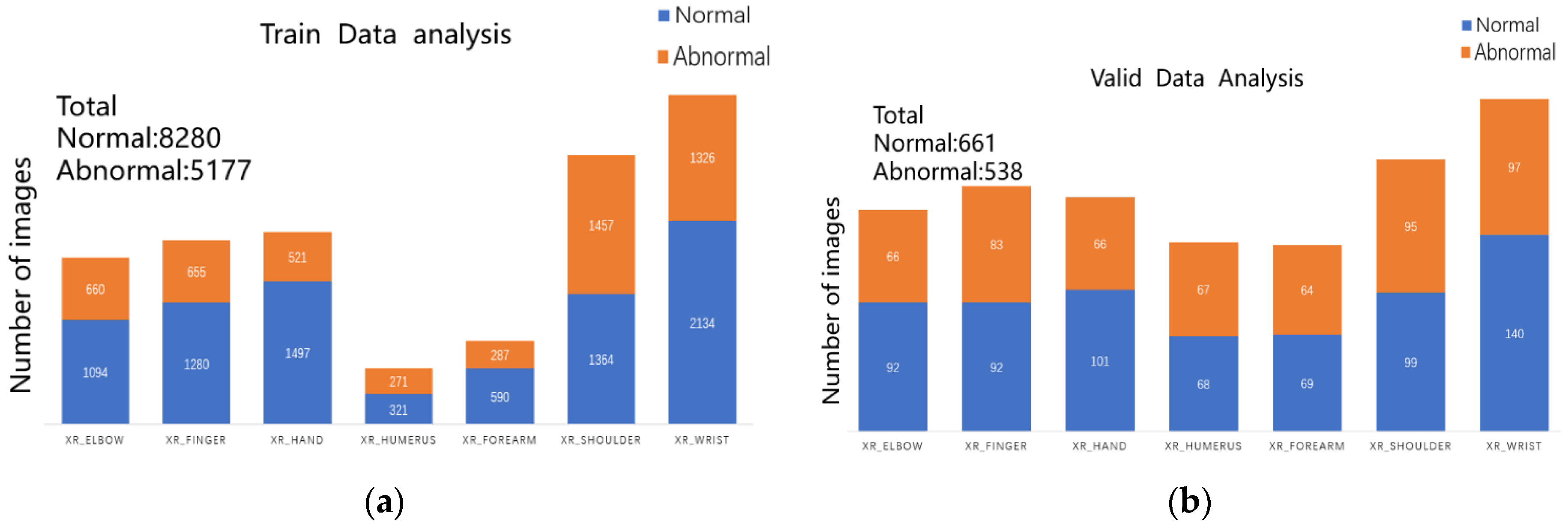
The MURA dataset [24] is the largest publicly available collection of musculoskeletal radiographic images, encompassing multi-view images of fingers, hands, wrists, forearms, elbows, humeri, and shoulders in the upper extremity region. It comprises 40,561 musculoskeletal radiographic images from 14,656 studies of 12,173 patients, with each study containing one or more radiographic images manually annotated by radiologists. This dataset is collected and released by the Stanford ML group as part of the Bone X-Ray DL Competition [24]. The training and validation sets consist of 13,457 and 1199 images, respectively, with the total number of images for each study type in the training and validation sets illustrated in Figure 1a,b.

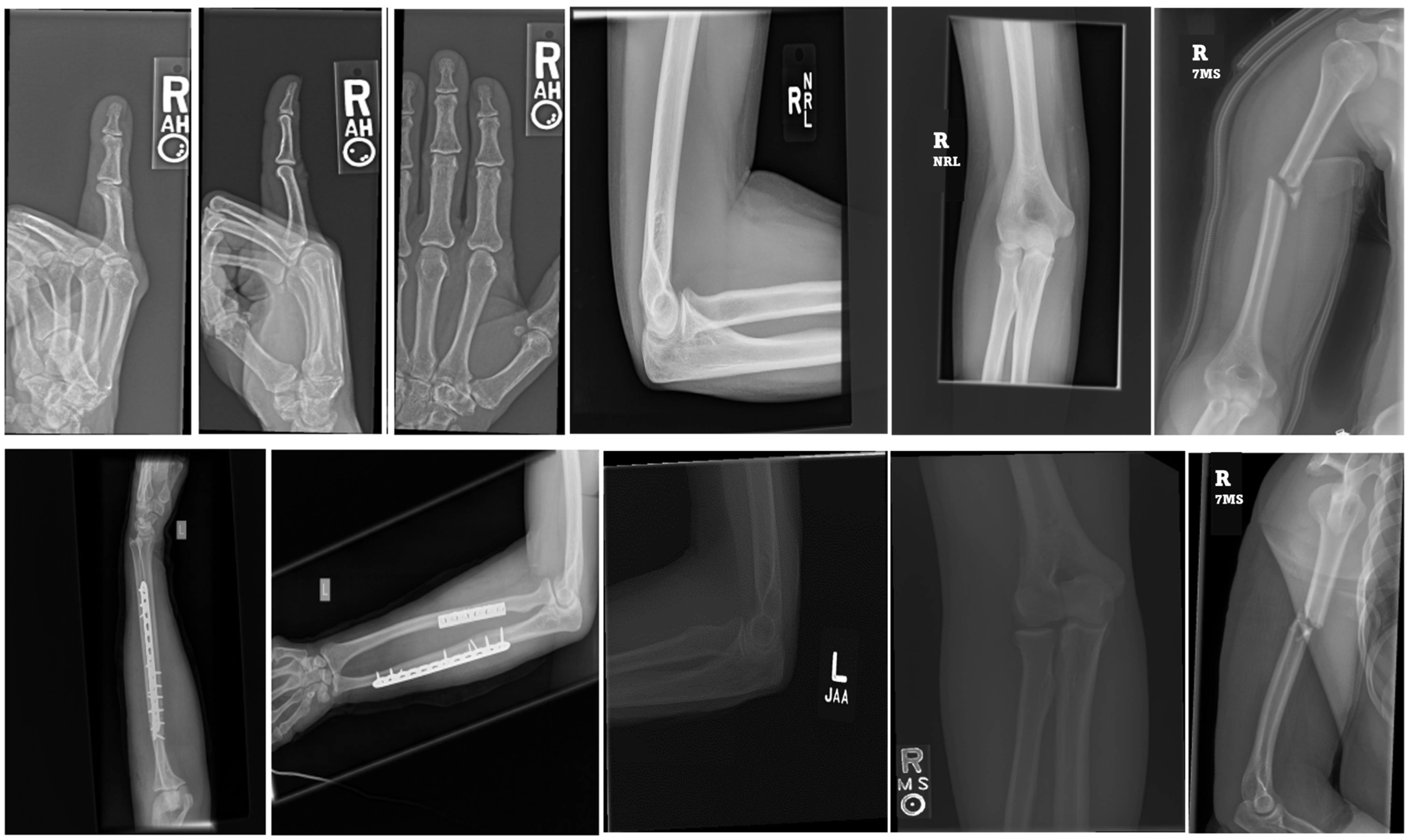
MURA classification is a binary task with labels represented as a 0–1 variable, where 0 indicates normal and 1 indicates the presence of an abnormality. In this dataset, there are 1912 studies of the elbow, 2110 studies of the fingers, 2185 studies of the hand, 727 studies of the humerus, 1010 studies of the forearm, 3015 studies of the shoulder, and 3697 studies of the wrist. For the test set, the majority vote of three radiologists serves as the gold standard. The official team trained a baseline model using a 169-layer DenseNet to detect and localize abnormalities, achieving an AUROC of 0.929, sensitivity of 0.815 at a working point of 0.815, and specificity of 0.887. When analyzing the dataset, we observed that each study had one or more images, with most studies having three images, as exemplified in Figure 2, an illustration of the MURA. dataset.

When utilizing the MURA dataset for training and validating the feasibility and accuracy of the model, it is also necessary to convert image data into tensors. In computer vision, images are typically composed of pixel matrices, with each pixel containing values for the red, green, and blue channels. Converting images to tensors is carried out to facilitate computer processing and analysis of the images. Typically, the pixel matrix of an image is represented as a three-dimensional tensor, where the first dimension denotes the number of channels, the second dimension represents the height of the image, and the third dimension represents the width of the image. Specifically, if the image is in color, it is often represented as a three-dimensional tensor with a shape of [3, H, W], where H is the height of the image, and W is the width of the image. If the image is grayscale, it can be represented as a three-dimensional tensor with a shape of [1, H, W]. Converting images to tensors is a common data preprocessing method in deep learning, typically performed before feeding the images into neural networks.

3. HRD Hybrid Model Construction

To solve the above problems, this study adopted mixed model theory, a convolutional neural network, and other related theories. The hybrid model proposed in this paper is composed of three modules: ResNet50, DenseNet121, and Human block, so this model is defined as the HRD model in this paper. The following sections mainly introduce the model from ResNet50, DenseNet121, Human block, and naive Bayes architecture.

3.1. ResNet50

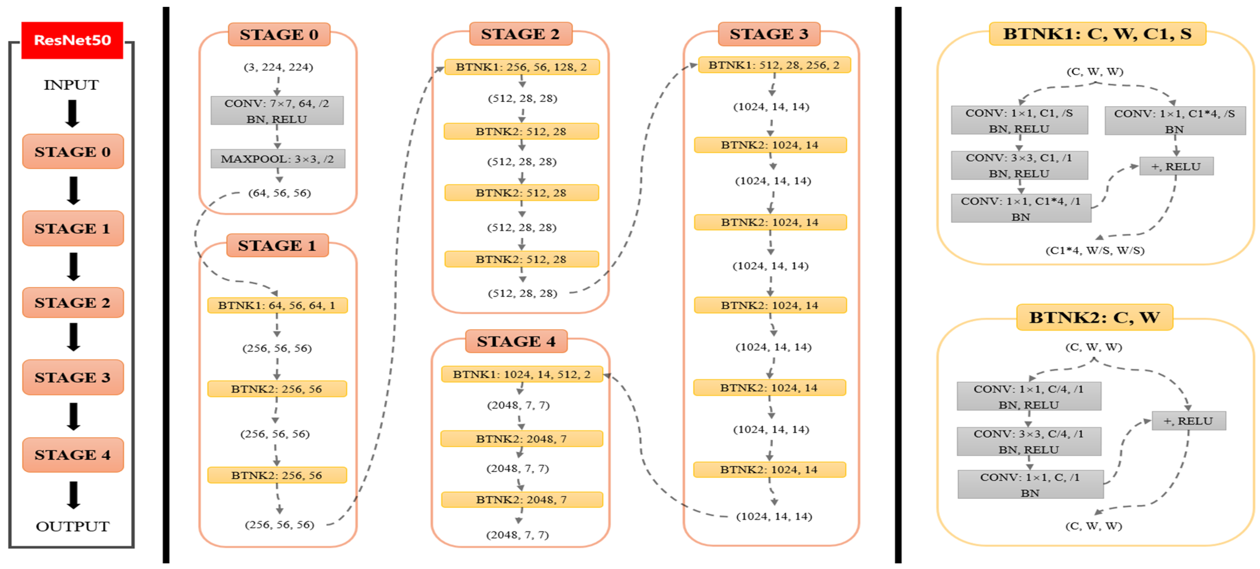
ResNet50 consists of 50 layers of convolutional neural networks including the convolutional layer, pooling layer, and fully connected layer. Unlike traditional convolutional neural networks, ResNet50 uses the idea of “Residual Learning” to solve the problem of network degradation by introducing a Residual Block, so that the network can be deeper and easier to train. Its structure is shown in Figure 3.

ResNet50 is trained by training strategy. The theoretical support of the training strategy is mainly based on deep learning optimization algorithms. In the training process of ResNet50, the optimization algorithm commonly used is Adam. It can adapt the learning rate adjustment, which can quickly converge and avoid the situation of shock. The formula of the Adam optimization algorithm is as follows:

$$\begin{array}{c}{m}_t={\beta }_t{m}_{t-1}+\left(1-{\beta }_1\right)g_t,\\ v_t={\beta }_2{v}_{t-1}+\left(1-{\beta }_2\right)g_t^2,\\ \widehat{m_t}=\frac{m_t}{1-{\beta }_1^t} ,\\ \widehat{v_t}=\frac{v_t}{1-{\beta }_2^t},\\ {\theta }_{t+1}={\theta }_t-\frac{\mu }{\sqrt{{\widehat{v}}_t}+ϵ}{\widehat{m}}_t\end{array}$$

(1)

where $m_t$ and $v_{t }$ represent the first and second moment estimates, ${\beta }_1$ and ${\beta }_2$ are decay rates, $g_t$ denotes the current gradient, $m_t$ and $\widehat{v_t}$ are bias-corrected estimates of the moments, $\theta$ denotes the learning rate, and $ϵ$ is a very small number to prevent division by zero.

Training process: After converting the image dataset into a tensor, we can input it into the ResNet50 model for training, which can be represented by the following mathematical formula:

Assume the input image is $X$ and the final output is $Y$. Each convolutional layer, pooling layer, fully connected layer, etc., can be considered as a function represented by $f_1, f_2, f_3, \dots , f_n$. The forward pass of the ResNet50 model can be expressed as:

$$Y=f_n\left(f_{n-1}\right(\dots f_3\left(f_2\right(f_1\left(X\right)\left)\right)\left)\right),$$

(2)

During the training process, cross-entropy was employed as the loss function in this study. Assuming the training dataset is D, the cross-entropy loss function L is defined as follows:

$$L_i=-y_i\mathit{log}\widehat{y_i}-(1-y_i)\mathit{log}(1-\widehat{y_i}),$$

(3)

where $y_i$ represents the actual label and $\widehat{y_i}$ represents the predicted result. The calculation formula for this loss function is based on the concept of cross-entropy in information theory. The intuitive interpretation is to maximize the probability of correct classification (i.e., to minimize the difference between the predicted result and the actual label). The overall calculation formula for the loss function throughout the training process is:

$$L=\frac{1}{n}{\sum }_{i=1}^n{L}_i,$$

(4)

where $n$ represents the total number of samples in the training set and $L_i$ represents the cross-entropy loss function for each sample. This loss function will be used for backpropagation, calculating gradients, and updating the model parameters.

After obtaining the value of the loss function (Loss), gradient descent is employed to reduce the L value, thereby improving the model’s classification capability. For the loss function L, gradients for each layer are computed using the chain rule. Specifically, for the j-th convolutional layer in the i-th layer, with output feature map $F_{i,j}$ and input feature map $F_{i-1,k}$, the gradient calculation formula for this convolutional layer is:

$$\frac{\partial L}{\partial F_{i-1,k}}={\sum }_j\frac{\partial L}{\partial F_{i,j}}\frac{\partial F_{i,j}}{\partial F_{i-1,k}},$$

(5)

where $\frac{\partial F_{i,j}}{\partial F_{i-1,k}}$ represents the gradient from the previous layer and $\frac{\partial L}{\partial F_{i,j}}$ is the derivative concerning the convolutional layer. Similar gradient calculation formulas can be used for batch normalization layers and fully connected layers. Therefore, the training process of the ResNet50 model can be expressed as follows. In the equations, $\theta$ represents the parameters of the model.

$$\mathit{min}\theta \frac{1}{\left|D\right|}{\sum }_{\left(x_i{y}_i\right)ϵD}L(y_i,f_n\left(f_{n-1}\left(\dots f_3\left(f_2\left(f_1\left(x_i\right)\right)\right)\right)\dots \right);\theta ),$$

(6)

Through the above formulas, the training process is illustrated in Figure 4. ResNet50 is divided into five stages, where Stage 0 has a relatively simple structure, serving as preprocessing for input data. The subsequent four stages are all composed of Bottleneck units and share a similar structure. Stage 1 contains three Bottleneck units, while the remaining three stages contain four, six, and three Bottleneck units, respectively. In Stage 0, the notation (3,224,224) represents the input data dimensions (channels, height, width). The input undergoes convolutional layers, batch normalization (BN) layers, ReLU activation functions, and MaxPooling layers, resulting in an output shape of (64,56,56). In this experiment, we modified the full connection layer of ResNet50 to two outputs to meet our binary classification task.

3.2. Densenet121

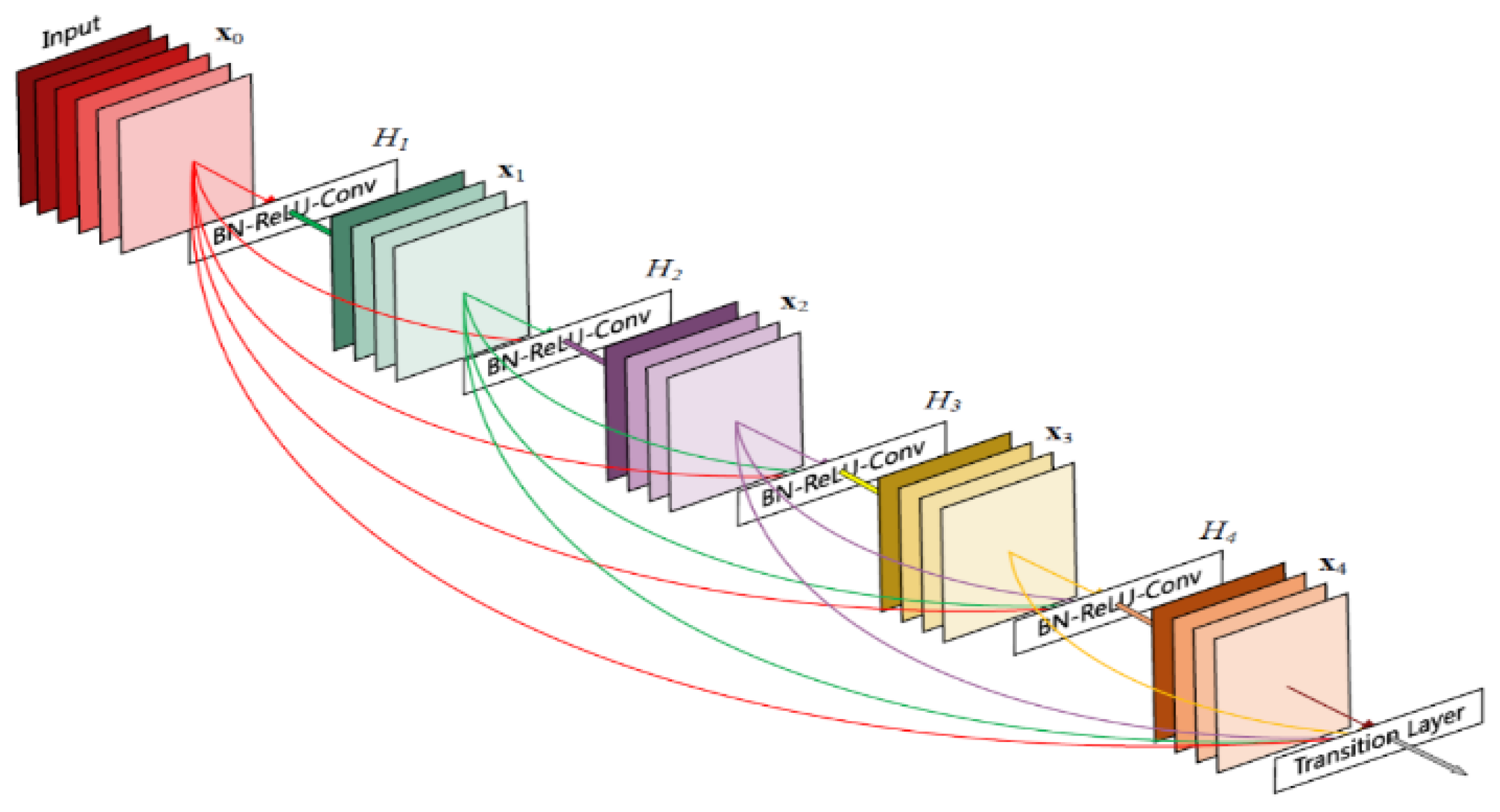
DenseNet121 consists of 121 layers of convolutional neural networks including dense blocks, transition layers, and global average pooling layers. Like ResNet, DenseNet uses cross-layer connectivity to enhance the delivery of information.

As shown in Figure 5, dense blocks are an important component of the DenseNet. In each dense block, the input feature graphs are successively processed through a series of convolution operations and nonlinear activation functions, and then the outputs of each convolution layer are spliced together to form a densely connected output. In this experiment, we changed the output of DenseNet’s fully connected layer to two to cater to our binary classification task.

Like ResNet50, DenseNet121 adopts the training strategy of the Adam optimizer. In the training process, the forward transfer formula of DenseNet can be expressed as follows:

$$\begin{array}{c}{x}_0=input,\\ x_l=H_l\left(\left[x_0,x_1,\dots ,x_{l-1}\right]\right),\end{array}$$

(7)

where $x_0$ is the input data, $x_l$ represents the output of the L-layer, and $H_l$ represents the nonlinear transformation of the L-layer. $[x_0, x_1,\dots ,x_{l-1}]$ indicates that the output from layer 0 to layer L − 1 is concatenated as the input of layer l. For layer l of DenseNet121, the input and output can be expressed as:

$$\begin{array}{c}{x}_0=input,\\ x_l=H_l\left(\left[x_0,x_1,\dots ,x_{l-1}\right]\right),\\ x_i=H_i\left(\left[x_0,x_1,\dots ,x_{i-1}\right]\right) 1\le i\le l-1,\end{array}$$

(8)

where $H_i$ represents the convolutional layer and nonlinear transformation in the i-th dense connected block and $\left[x_0, x_1,\dots ,x_{i-1}\right]$ represents the concatenation of the output of the previous i − 1 layer as the input of the i-th dense connected block. The backpropagation formula of DenseNet can be expressed as:

$$\frac{\partial L}{\partial x_l}=\frac{\partial L}{\partial H_l}\left(\left[x_0,x_1,\dots ,x_{l-1}\right]\right)+{\displaystyle {\sum }_{i=0}^{l-1}}\frac{\partial L}{\partial x_i}\frac{\partial x_i}{\partial x_l},$$

(9)

where L represents the loss function; the rest of the definitions are referred to above.

3.3. Human Block

In the hybrid model, we aimed to facilitate interaction between the model and individuals, enhancing the model’s generalization capabilities and refining its accuracy through iterative learning with human input. Consequently, within the Human Block module, we engaged in the tensor processing of human judgments on images, converting them into a computationally manageable format suitable for computer input. Given the inherent uncertainty and stochastic nature of human diagnostic quality, we employed a function within this module to better align the model with human diagnostic input and bolster its resilience. This function’s parameters span from 0.0 to 1.0, simulating human diagnostic accuracy. During each batch of model training, the function incorporates dataset labels into the batch and selectively alters some labels based on pre-established accuracy criteria. The introduction of bias within the function induces a ±2.5% fluctuation in model training accuracy, effectively mirroring the stochastic characteristics of human diagnosis. Crucially, the function randomly alters labels, effectively emulating human diagnostic processes and circumventing systematic biases that could lead to overfitting. 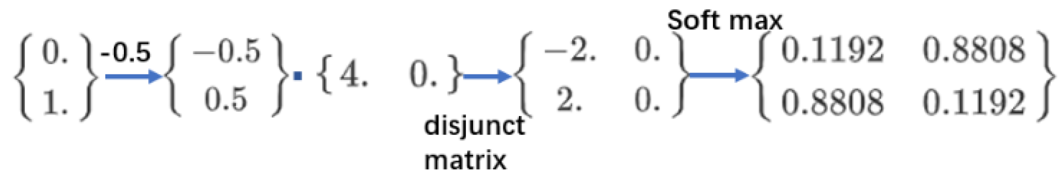As shown in Figure 6, the X-ray image is first given a prediction and then probabilistically processed as input data into the naive Bayesian model. As shown in Figure 7, a set of evaluation inputs is represented as 0–1, then the corresponding subtraction and dot multiplication operations are performed, and finally, the probability value is obtained through the operation of the softmax function in the second dimension. Importantly, these probability values are calibrated against average human prediction accuracy, with a single set of probabilities serving as the standard for demonstration.

Furthermore, to assess the model’s robustness and gauge the influence of human diagnostic accuracy on model outcomes, additional experiments were conducted. These experiments involved adjusting parameters to maintain human diagnostic accuracies at approximately 60%, 70%, and 75%, respectively, while subjecting the models to testing. The experimental findings are depicted in the accompanying Figure 8. Across the three depicted stages, the final model accuracy exhibited a corresponding increase alongside improvements in human diagnostic accuracy, with model accuracy consistently maintained within the range of 80% to 90%. This observation underscores the hybrid model’s robustness and its significant potential for enhancing the accuracy of musculoskeletal disease identification. Moreover, it highlights the model’s ability to provide valuable assistance to clinicians in achieving the rapid and efficient diagnoses of musculoskeletal diseases.

3.4. HRD Hybrid Model Construction

In the proposed hybrid model in this paper, each image is initially fed into ResNet50 and DenseNet121. The respective feature representations are obtained, and these representations are concatenated and used as input for the naive Bayes model. This paper assumes that each feature is conditionally independent of the class. The Bayesian formula is then applied to calculate the probability of each class, and the class with the highest probability is selected as the final classification result. The parameters mainly include prior probability P(Y) and conditional probability P(X|Y), where X represents the input feature vector and Y represents the output classification label. Maximum likelihood estimation is used to estimate these parameter values based on the training dataset, optimizing the model’s classification performance on the training set under these parameters. Based on the training dataset, we can estimate the prior probability P(Y) for each classification label as follows:

$$P\left(Y=c\right)=\frac{{\sum }_{i=1}^{N}I(y_i=c)}{N},$$

(10)

where N represents the size of the training dataset, $y_i$ represents the true classification label of the i-th sample, and i is the indicator function with a value of 1 when the condition in the parentheses is true, and 0 otherwise.

Next, for each classification label, estimate the conditional probability P(X|Y = c) for its feature vector X. Since the feature vector X is continuous, it can be modeled using a Gaussian distribution, that is:

$$P\left(X_j=x_j|Y=c\right)=\frac{1}{\sqrt{2\pi {\sigma }_{jc}^2}}\mathrm{e}\mathrm{x}\mathrm{p}(-\frac{{(x_j-{\mu }_{jc})}^2}{2{\sigma }_{jc}^2}),$$

(11)

where $x_j$ represents the value of the j-th component of the eigenvector X, and ${\mu }_{jc}$ and ${\sigma }_{jc}$ represent the mean and variance of the j-th feature under the classification label c, respectively. Finally, according to the Bayes formula, the posterior probability P(Y = c|X) of the input feature vector X under each classification label can be calculated, and the classification label with the greatest posterior probability can be selected as the output result.

$$\widehat{y}=\underset{c}{\mathit{argmax}}P(Y=c){\prod }_{j=1}^{d}P(X_j=x_j|Y=c),$$

(12)

The overall structure diagram of the HRD hybrid model proposed in this paper is shown in Figure 9. For X-ray image data, on the one hand, the image data are converted into a tensor, and then the data are passed into the trained neural network model. On the other hand, the image data are handed over to people for processing, and the specific classification data (0–1 variable) is given, then converted into the predicted probability value by Human Block. Finally, the prediction probability values of the three blocks are summarized, and the concrete prediction values of the image are given by the naive Bayes model.

4. Experiments and Results

To validate the effectiveness and accuracy of the proposed hybrid model, feasibility experiments were conducted using the MUAR dataset as previously mentioned in this paper. Accuracy, recall, F1-score, ROC curve, and AUC value were adopted as evaluation metrics. These metrics will aid in assessing the model’s performance and verifying the efficiency of the proposed hybrid model, along with the feasibility of the hybrid strategy through comparisons with various baseline models. The following models will be included in the comparison: ResNet50 and Densenet169.

4.1. Accuracy Rate

The HRD and baseline models were evaluated under the same settings in this study. All models were trained using identical strategies, and the model with the minimum cross-entropy loss after training was selected for evaluation. As shown in

Table 1. Accuracy of each model.

	Resnet50	Densenet169	HRD-Model
XR_ELBOW	0.815	0.823	0.884
XR_FINGER	0.764	0.781	0.837
XR_FOREARM	0.783	0.805	0.845
XR_HAND	0.746	0.784	0.833
XR_HU ERUS	0.843	0.863	0.885
XR_SHOULDER	0.771	0.773	0.816
XR_WRIST	0.803	0.834	0.867

, HRD demonstrated higher accuracy than both baseline models across all types of X-ray images. For ResNet50, HRD exhibited an accuracy improvement ranging from 4% to 9%, and for DenseNet169, HRD showed an accuracy improvement ranging from 2% to 6%. This indicates the effectiveness of the hybrid model. However, evaluating a model’s performance should not solely rely on accuracy, especially in an imbalanced dataset. Therefore, the assessment will continue by considering additional metrics.

4.2. Confusion Matrix

When testing the mixed model and the baseline model, the confusion matrix can better understand the performance of the model in various categories. The accuracy rate, recall rate, and accuracy rate of the mixed model and the baseline model can be obtained through the confusion matrix to compare the performance differences between the two models. The confusion matrix of each model in various X-ray images is shown in

Table 2. Classification results of each model.

TP	FN	ResNet50		DenseNet169		HRD-Model
FP	TN
XR_ELBOW		218	17	204	31	211	24
		73	157	47	183	41	189
XR_FINGER		178	36	176	38	191	23
		82	165	70	177	71	176
XR_FOREARM		132	18	139	11	141	9
		51	100	48	103	43	108
XR_HAND		240	31	245	26	252	19
		91	98	86	103	78	111
XR_HUMERUS		121	27	120	28	128	20
		21	119	22	118	16	124
XR_SHOULDER		224	61	217	68	227	58
		67	211	76	202	58	220
XR_WRIST		336	28	328	36	330	34
		88	207	74	221	69	226

, where TP, TN, FP, and FN represent the results after classification by each model, namely true cases, true negative cases, false positive cases, and false negative cases, respectively. The equation related to the confusion matrix is as follows:

$$\begin{array}{c}Precision=TP/(TP+FP),\\ Recall=TP/(TP+FN),\\ F1-Score=2\ast Precision\ast Recall/(Precision+Recall),\end{array}$$

(13)

4.3. Precision

Precision ratio is one of the indices to evaluate the performance of the binary classification model. It represents the proportion of the samples predicted by the model as positive examples. The precision ratio of the baseline model and HRD in this experiment are shown in

Table 3. The precision ratio of each model.

	Resnet50	Densenet169	HRD-Model
XR_ELBOW	0.7491	0.8127	0.8394
XR_FINGER	0.6846	0.7154	0.7318
XR_FOREARM	0.7213	0.7433	0.7637
XR_HAND	0.7251	0.7472	0.7652
XR_HU ERUS	0.8521	0.8451	0.8881
XR_SHOULDER	0.7698	0.7406	0.7993
XR_WRIST	0.7925	0.8159	0.8234

.

It can be found that HRD achieved a higher accuracy than ResNet50 and DenseNet169 in all X image types, indicating that the mixed model had a better classification effect on the MURA dataset than the single ResNet50 and DenseNet169 models. As can be seen from the table, HRD performed best in the test set of type XR_HUMERUS, with accuracy improvements of 4.4% and 4.5% over the ResNet50 and DenseNet169 models, showing the advantages of the hybrid model in some cases.

4.4. Recall

Recall is one of the indicators used to measure the performance of a classification model, which refers to the ability of a classifier to correctly identify all positive samples. The recall rates of various models are shown in

Table 4. Recall rate of each model.

	Resnet50	Densenet169	HRD-Model
XR_ELBOW	0.9277	0.8681	0.8979
XR_FINGER	0.8318	0.8224	0.8925
XR_FOREARM	0.8800	0.9267	0.9400
XR_HAND	0.8856	0.9041	0.9299
XR_HU ERUS	0.8176	0.8108	0.8649
XR_SHOULDER	0.7860	0.7614	0.7965
XR_WRIST	0.9231	0.9011	0.9066

.

Based on the recall metrics, HRD outperformed ResNet50 and DenseNet169 in most categories.

4.5. Comprehensive Comparison of Accuracy Rate and Recall Rate

As can be seen from the confusion matrix shown in Figure 10, HRD was superior to the ResNet50 and DenseNet169 baseline models in the diagnosis of true cases and true negative cases, with a recall rate 2% and 3% higher than that of the Resnet50 and Densenet169 baseline models, and a precision rate 4% and 3% higher, respectively. Therefore, the accuracy rate and recall rate were also higher than the baseline model, indicating that HRD can classify X-ray images more effectively and reduce the occurrence of misdiagnosis.

4.6. F1-Score

The F1-score takes the accuracy and recall into account, giving equal weight to both, so that the performance of the model can be evaluated more comprehensively.

Table 5. F1-score table of each model.

	Resnet50	Densenet169	HRD-Model
XR_ELBOW	0.783	0.812	0.877
XR_FINGER	0.747	0.758	0.799
XR_FOREARM	0.745	0.786	0.832
XR_HAND	0.628	0.655	0.697
XR_HU ERUS	0.831	0.829	0.878
XR_SHOULDER	0.773	0.747	0.793
XR_WRIST	0.783	0.800	0.812

shows the F1-score table of each model.

Compared with the baseline model, the HRD model could maintain high accuracy while considering the high recall rate of positive examples, that is, it can strike a balance between the accuracy and recall rate, and at the same time, has a better classification ability.

4.7. ROC Curve and AUC Value

The ROC curve is a graphical presentation used to evaluate the performance of a binary classification model. The ROC curve shows the relationship between the TP rate and the TF rate. The AUC value is the area under the ROC curve and represents the probability that the classifier will rank the positive sample ahead of the negative sample. The larger the AUC value, the better the performance of the classifier. AUC values range from 0.5 to 1, where 0.5 means a random classifier and 1 means a perfect classifier. The AUC value can be used to evaluate the performance of the binary classification model, especially in the case of imbalance in the ratio of positive and negative samples, as the AUC value is more accurate because the AUC value is not affected by the sample proportion.

This article used the XR_HAND category as an example, as shown in Figure 10 and

Table 6. AUC values of each model.

	Resnet50	Densenet169	HRD-Model
XR_ELBOW	0.87	0.89	0.94
XR_FINGER	0.85	0.85	0.91
XR_FOREARM	0.84	0.87	0.93
XR_HAND	0.80	0.84	0.91
XR_HU ERUS	0.86	0.90	0.95
XR_SHOULDER	0.84	0.84	0.92
XR_WRIST	0.83	0.89	0.94

. Experiments showed that taking the ROC curve and AUC value as indicators, compared with the baseline model, the ROC curve was closer to the upper left corner and the AUC value was higher, indicating that HRD has a better classification performance and effect. Compared with HRD, the baseline model was closer to the 45-degree line in different degrees, and the AUC value was significantly lower than that of HRD. The two sets of baseline models have their advantages and disadvantages in different classifications, so the improved naive Bayes model can consider the advantages of both.

4.8. Cohen’s Kappa

In this study, the role and use of Cohen’s kappa values were also added. Cohen’s kappa values provide insights into the consistency between the predicted and true labels and are particularly valuable in cases where the dataset is unbalanced. Cohen’s kappa values provide insights into the agreement between the predicted labels and the ground truth labels, particularly valuable in scenarios with imbalanced datasets. The results of the Cohen’s kappa values of the three models on different types of X-ray images are shown in

Table 7. Cohen’s kappa of each model.

	ResNet50	DenseNet169	HRD-Model
XR_ELBOW	0.689	0.697	0.796
XR_FINGER	0.625	0.645	0.730
XR_FOREARM	0.647	0.674	0.736
XR_HAND	0.580	0.636	0.711
XR_HUMERUS	0.731	0.766	0.795
XR_SHOULDER	0.627	0.638	0.695
XR_WRIST	0.659	0.711	0.767

.

The Cohen’s kappa values demonstrate the level of agreement between the models’ predictions and the actual labels, providing a more comprehensive assessment of model performance, particularly in situations where accuracy alone may not suffice. Additionally, a comparison between the three models based on Cohen’s kappa values revealed that the HRD model consistently outperformed both ResNet50 and DenseNet169 across all types of X-ray images, indicating its superiority in capturing the agreement between the predicted and ground truth labels.

4.9. Mixed Model Strategy

This paper also focused on the effectiveness of mixed model strategies. For example, machine learning models generate preliminary results, which are then reviewed and corrected by human experts or artificial intelligence systems that analyze and mine large amounts of data, then human experts make decisions based on the analytical results. In this paper, the submodels ResNet50 and DenseNet121 in HRD were taken out and combined with Human Block in pairs to test whether the hybrid strategy is effective, as shown in Figure 11. It is biased for a classification model to simply consider the accuracy of the model on the test set. Therefore, this paper adopted the same verification strategy as above, and formulated the confusion matrix, accuracy rate, recall rate, F1-score, ROC curve, etc. of various mixed models. Figure 12 shows the AUC values for the various hybrid models.

Using ResNet50 and DenseNet121 as benchmarks, it was found that the accuracy and AUC value of any combination strategy containing ResNet50 was significantly better than that of a single ResNet50 model. In the XR_SHOULDER and XR_HAND categories, the accuracy and AUC values were significantly improved when combined with either module. In all categories, the combination of ResNet50 with Human Block outperformed DenseNet169 in accuracy and AUC values, while the combination with DenseNet121 also had higher accuracy and AUC values. Similarly, the combination strategy experiment based on DenseNet121 also reached a similar conclusion, that is, the combination of small models could reach or even surpass the performance of large models, thus verifying the rationality of the mixed model strategy.

For any two model combinations, the hybrid model could improve the accuracy and AUC value. In particular, the performance of the combined model of ResNet50 and DenseNet121 was no worse than that of DenseNet169 under the condition of less computation, which further verifies the correctness of adopting the mixed model strategy.

5. Conclusions and Limitations

In this study, our primary focus centered on the application of deep learning methodologies in the diagnosis of musculoskeletal (MSK) diseases. Leveraging the MURA dataset, we constructed a hybrid neural network architecture to assess the model’s performance, subsequently analyzing the experimental outcomes. Our findings underscore the considerable promise of deep learning methodologies augmented by human involvement, showcasing their potential applicability across diverse practical domains. Examples include but are not limited to spam filtering, misinformation detection on public platforms, and industrial anomaly detection, where the integration of deep learning models with human inputs significantly enhances the data accuracy and efficacy.

Within our experimental framework, the HRD hybrid model exhibited prediction accuracies ranging between 75% and 90%. Notably, in real-world scenarios, the model can be easily tailored to accommodate various levels of diagnostic accuracy within the Human Block, thereby facilitating medical diagnosis for novice and general practitioners alike, boasting a simplicity of deployment and operational efficiency. Moreover, comparative analysis revealed that the hybrid model outperformed its single-model counterparts across multiple metrics, demonstrating superior generalization capabilities and classification accuracy.

Nevertheless, the study findings exhibited less discernible impact among the senior physicians specializing in musculoskeletal disease diagnosis. Future research endeavors could explore the replacement of the ResNet50 and DenseNet121 models within the proposed hybrid framework, potentially yielding a more optimized hybrid model. Furthermore, while the present study categorized X-ray image results into binary classifications (i.e., abnormal or normal), future investigations could delve into finer-grained categorizations of abnormal conditions such as fractures, strains, arthritis, etc.

Importantly, the study overlooked crucial environmental factors, suggesting avenues for future exploration. Incorporating uncertainty estimation techniques such as Monte Carlo dropout could bolster the methodological robustness, reliability, and practical applicability within clinical settings, particularly in critical medical scenarios.

While our study validated the feasibility of the HRD hybrid model, its efficacy, robustness, and generalization capabilities in identifying musculoskeletal abnormalities warrant further enhancement. Through iterative refinement and adjustment of the model, we aspire to elevate the hybrid model to a gold standard in lesion detection, potentially alleviating diagnostic burdens associated with MSK conditions and facilitating expedited and accurate patient treatment.