Influence of Site Effects on Scaling Relation Between Rotational and Translational Signals Produced by Anthropogenic Seismicity

Abstract

The measurements of rotational and translational seismic signals were carried out at the Imielin and Planetarium stations located in the central part of the Upper Silesian Coal Basin, Southern Poland. Local seismicity, produced by the surrounding hard coal mines, allowed the collection of 130 seismic events. This study aimed to analyze the influence of site effects on rotational ground motion using the horizontal-to-vertical spectral ratio method. We performed the analysis using two approaches: obtaining the spectral ratio of the rotational motion and investigating the impact of the site effect on the scaling relation. The spectral ratio comparison between rotations and translations shows that the value of the rotational amplification coefficient is almost three times lower than that for the translations, and the resonance frequency of rotational motion is higher than that of translations. The comparisons of the scaling relation models, obtained for raw data and corrected by the amplification factor data, revealed that removing the site effect from the signals increases the data to model approximation, reducing the value of the SH-wave phase velocity almost three times. The studies suggest that the local site conditions independently affect the rotational and translational motions.

1. Introduction

Rotational ground motion is described by three components: torsion, as motion around a vertical axis, and rocking—around two horizontal axes [1]. Generally, rotational seismology is used to study the effects of natural seismicity [2,3,4,5,6], but the influence of anthropogenic seismicity has also been taken into consideration in the last decade [7,8,9]. Separate topics concern the rotation-to-translation scaling relations or transformations [10,11] and the generation of a specific sequence of translational and rotational motions in anisotropic media [12,13]. In addition, one should note that concerns about the effects of rotational motions on civil structures [14,15,16,17] and their potential responsibility for the instability of the failure mechanism of landslides and slopes [18,19] have increased significantly over the past two decades. Nevertheless, one poorly documented issue still needs to be addressed: the relation between rotation and site conditions. Regarding the translations, the site effect parameters can be estimated using the horizontal-to-vertical (H/V) spectral ratio method [20]. Further research has shown that the H/V method can be used to estimate the rotational site effect parameters after rewriting the equations [11,21,22,23,24]. The new formula assumes the torsion-to-rocking spectral ratio (TRSR) estimations, which correspond to the horizontal rotation spectrum to the vertical rotation spectrum [11,21,22,23,24]. The explanation for rewriting the original H/V formula is motivated by the fact that torsion represents motion in the horizontal plane, while rockings are motions in the vertical plane [21]. In the literature, one can find comparisons of the rotational and translational amplification spectrum performed for the rotation of the registered components [23] and related to estimating the spectrum ratio [24]. However, given that the amplification effect and the resonance of the wave in the ground affect the observed translational and rotational signals [22,23,24], the parameters of the scaling relation between the rotational and translational peak values should also be affected by the site effect [4,5,9,11,25,26,27]. The main contributions of the current research are as follows:

• Investigated the possibility of estimating the site effect parameters of rotational motion using the rewritten horizontal-to-vertical spectral ratio method and comparing the obtained results to the translational motion.
• Estimated the scaling relation between the maximum peak values of horizontal ground acceleration (PGA) and vertical rotational velocity (PRV) for two models, y = ax and y = ax + b, checking whether the intercept b is significant and what physical meaning it may have.
• Analyzed the influence of amplification on the scaling relation function by re-estimating the models for amplification factor-corrected data sets.

The rest of the manuscript is arranged as follows: Section 2 presents a detailed description of the site conditions, seismic data characteristics, and applied methods; Section 3 presents the results of the analysis; Section 4 explores the discussion part of the paper; and finally, Section 5 concludes the study.

2. Materials and Methods

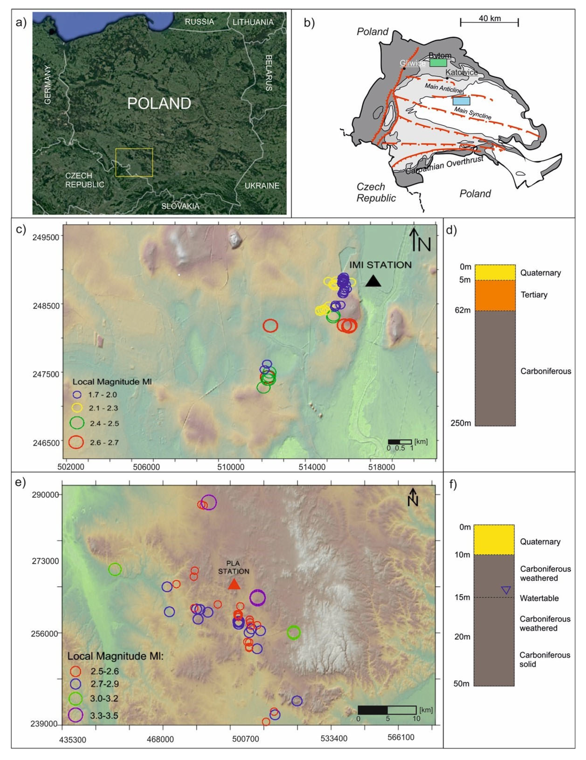
2.1. Site Conditions

The IMI station was installed near the Dziećkowice water reservoir and two mines: the Sobieski Mine and the Ziemowit Mine in the Upper Silesian Coal Basin (USCB), Poland (Figure 1).

The PLA station was located in the City of Chorzów, in the central part of the USCB, and recorded events from mines located at greater distances, such as the Bielszowice Mine, the Murcki-Staszic Mine, and the Sośnica Mine. The study presented here deals with the site effects; hence, we investigated the local geology from a physical perspective for a three-layered model: loose material (subsoil), intermediate layer, and rigid basement (Figure 1d,f). The rigid basement for both station sites is a Carboniferous coal-bearing formation built mainly of sandstones, mudstones, and siltstones interbedded with hard coal seams [27,29,30]. The upper depth level of the rigid basement reached 62 and 10 m for IMI and PLA station sites, respectively. The intermediate layer, which exists in the IMI station, is represented by weathered Triassic sandstones (Buntsandstein), which reach a thickness of 52 m (Figure 1d). This layer is intermediate because its elastic properties are between rigid and loose material due to the strongly weathered rocks [28,31]. A similar intermediate layer is present beneath the PLA station. However, this resonant layer is approximately 15 m thick and comprises Carboniferous rocks, which are strongly weathered and fractured, and near-surface sediments are 5 m thick clay (Figure 1f). The top layer near the stations comprises Quaternary sediments (Figure 1d,f), represented by a mix of sand, pebbles, mud, alluvia, and peats [28,31]. The physical properties of the subsurface have already been investigated. The average S-wave velocity value for the IMI and PLA at a depth of 30 m (Vs30 parameter) below ground level was 408 m/s and 512 m/s, respectively, as obtained from The Multichannel Analysis of Surface Waves (MASW) [9].

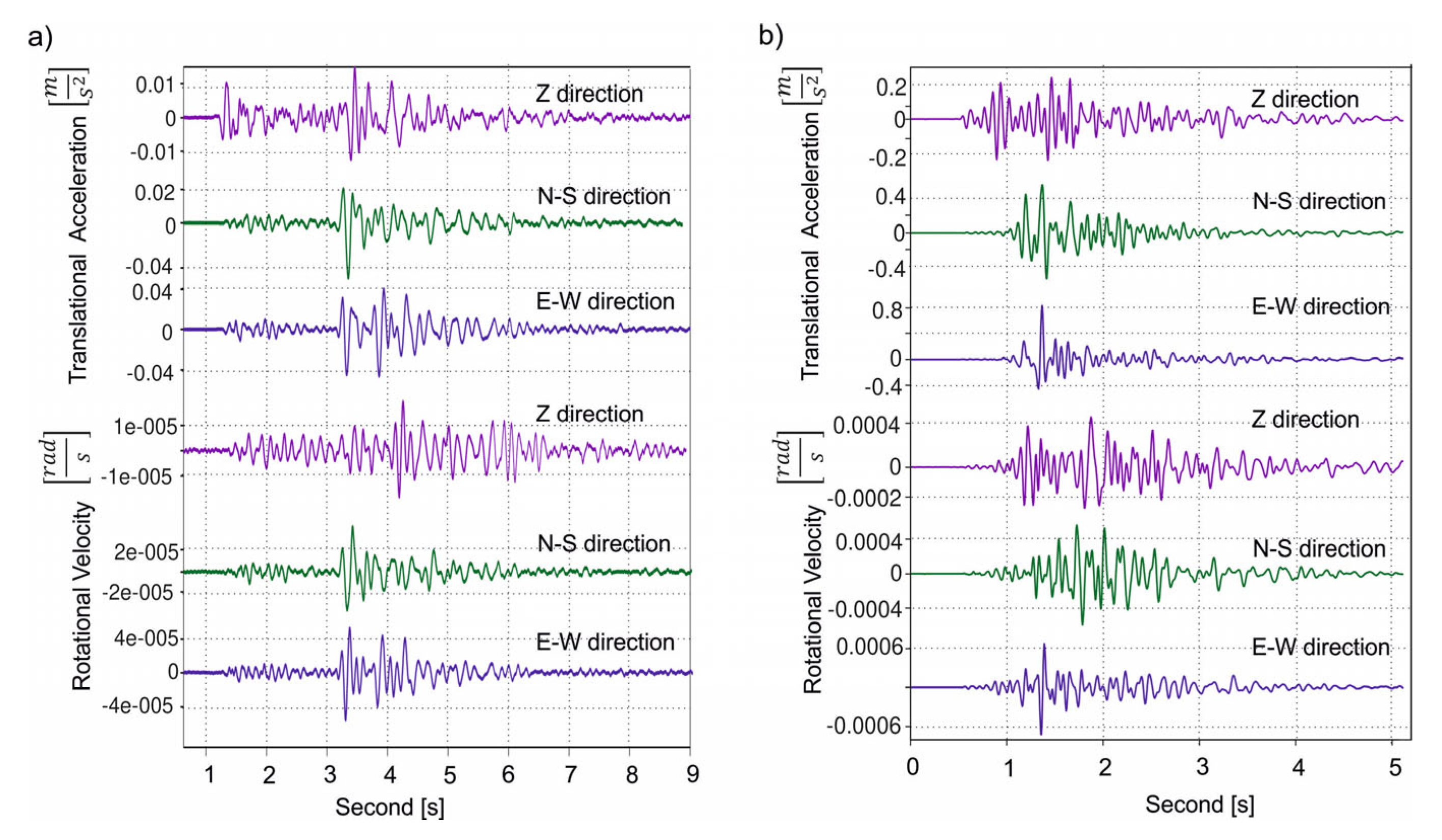
2.2. Data and Sensors

The Upper Silesian Coal Basin, known as a seismically active mining area, is mainly characterized by two general types of events: mining-related and mining-tectonic seismicity [32]. Seismic events exclusively associated with mining have relatively low energy and occur near mine roadways. In contrast, tectonic-related events generally have higher energy and are generated in dislocation zones, often far from mine working sites. The focal mechanism of mining seismicity events is generally characterized by a relatively small shear component compared to the explosive and compressional components. The opposite situation was noticed in the case of the mining-tectonic seismicity, where the shear component reached 70% of the total seismic moment tensor solution, corresponding to the double-couple source mechanism. The seismic signals from the seismic data collected at both sites were characterized by peak motion values at the S-wave phase. They were, therefore, considered to be the effect of mining-tectonic seismicity. During the seismic observations, 60 events occurred at the IMI station site. The strongest of these, whose local magnitude reached ML 2.7, occurred on 24 June 2015. In the catalogue, the local magnitudes of the events range from 1.7 to 2.7 at distances ranging from 0.74 to 5.6 km (

Table 1. Characteristics of the analyzed seismic events.

Energy [J]	ML	IMI STATION		PLA STATION
		Number	Epicentral Distance for the Energy Range [km]	Number	Epicentral Distance for the Energy Range [km]
1.0 × 105–5.0 × 105	1.7–2.0	35	0.75–5.13	0	-
6.0 × 105–9.9 × 105	2.1–2.3	13	0.65–1.42	0	-
1.0 × 106–5.0 × 106	2.4–2.5	7	1.17–5.52	22	5.68–18.99
6.0 × 106–8.5 × 106	2.6–2.7	5	1.34–4.20	28	5.63–18.32
1.3 × 107–2.4 × 107	2.8–2.9	-	-	12	5.67–20.43
3.2 × 107–7.6 × 107	3.0–3.2	-	-	5	5.91–12.38
1.2 × 108–2.8 × 108	3.3–3.5	-	-	3	8.20–9.70

). All event sources were located in the SSW direction with respect to the seismological station. Relatively large events occurring at a short distance of only 1 km from the seismological station in Imielin result in a high resolution of the seismic signal (Figure 2a).

Seventy events were noticed at the field of the PLA station. The strongest one occurred on 3 June 2016, and its magnitude reached ML 3.4. The catalogue contains events with local magnitudes ranging from 2.5 to 3.4 at a distance ranging from 5.7 to 20.4 km (Table 1). The event sources are located mainly in the NEE direction relative to the seismological station. The distance between the source and the station is higher than in the IMI station, but the seismic energy is also relatively higher. Therefore, the signal resolution is comparable to the second station (Figure 2b). Each analyzed event (Figure 1c,e) was registered by the EENTEC measuring set, composed of the seismic recorder DR-4000 linked to the GPS module, translational accelerometer EA-120, and rotational seismometer R-1. EA-120 is a triaxial force-balanced accelerometer with a scale range equal to ±2 g and a dynamic range equal to 128 dB. R-1 is a well-known triaxial rotational seismometer, the resolution of which is equal to 1.2 × 10⁻⁷ [rad/s], with a dynamic range equal to 110 dB, frequency band ranging from 0.05 to 20 Hz, and amplitude clip at the level of 0.1 rad/s at 1 Hz [33]. In the case of the PLA station, the sensors were mounted in the basement at a concrete pedestal, while in the IMI station, the sensors were deployed in a thin vault at 1.20 m depth. The temperature in both places was stable and lower than 18 °C, which helped avoid problems with the measurement reliability of the rotational sensor [34]. The sensor channel orientation was X- in the East–West direction, Y- in the North–South direction, and Z-axis in the vertical direction. The seismic catalogue of registered events, which contained the data related to the location and energy, was prepared based on the records from the IS-EPOS (European Plate Observing System) platform, a unit of the Upper Silesian Geophysical Observation System [35]. The waveforms, including translational acceleration and rotational velocity signals, were processed using the Butterworth filter in the ca. 1 Hz to 20 Hz frequency range and filter order equal to 6.

2.3. Site Effect

Studies of site effects are elaborate and well-known, starting with the study by Nakamura [20]. The resonance frequency of the near-surface layer and the corresponding amplification coefficient are the two main parameters of site effects. In the case of two-layered geology represented by loose sediment and rigid basement, the resonance frequency is related to the former layer (Figure 3c). However, geology is usually complex; the resonating layer can combine many layers of different geology and elastic properties. The resonance frequency largely depends on the thickness of this resonating layer, which acts as a bandpass filter that enhances selected frequencies. The amplification coefficient shows how many times amplitudes are amplified; thus, it can affect the registered signals by increasing the registered amplitudes for specific frequencies. The amplification increases as the impedance between stiff and loose rocks increases (Figure 3c). The empirical method allowing to find the site effect parameters is the horizontal-to-vertical spectral ratio (HVSR) technique, based on a spectral ratio of translation amplitude recorded for two main directions (Figure 3a): horizontal, H, and vertical, V [36,37,38,39,40].

2.3.1. Theoretical HVSR

The site effects can also be estimated using predictive theoretical formulas. The H/V ground motion spectrum was calculated for the one-dimensional model of horizontal layers, considering vertically propagating shear waves. Such an assumption results from analyzing seismograms from the research area, where S-type waves transmit most seismic energy. Each layer is homogeneous and isotropic and is characterized by thickness, density, shear modulus, and damping coefficient. In our cases, the shear velocity to calculate shear modulus was taken from seismic surveys and the presented geological profiles (Figure 1d,f). In this study, we applied the formula from the paper of Szczygieł [4]. The theoretical calculation uses dependencies between acoustic impedance, absorption/attenuation coefficient, soft layer thickness, shear velocity in soft and rigid layers, and the shock-wave frequency. The maximum value of the calculated H/V ratio corresponds to the amplification coefficient and the expected resonance frequency. This theoretical relation assumes that the layers are infinite in their lateral extent and, hence, should be considered a steady-state approximation of the site effect parameters [41,42]. The HVSR method tends to underestimate the value of the amplification coefficient of the ground motion in comparison to the classic standard spectral ratio [43,44]. Moreover, the HVSR spectrum can present more than one significant peak, leading the subjective analysis to accept the first (fundamental) or highest peak as the determinable resonance frequency [44]. Therefore, the theoretical models were estimated to avoid potential inaccuracies in analyzing the HVSR result.

2.3.2. Empirical HVSR

The site effect coefficients and the empirical HVSR analysis, using single station measurements, have so far only been studied using translational motion recordings but not for rotation. Therefore, we adapted the HVSR method to rotation in this study, considering the opposite direction of motions. The rotational motion is described as the curl of three components: the torsion (around the vertical axis) and two components of rocking (around the horizontal axis). The planar orientation of the rotational components allowed us to estimate the rotational HVSR as the torsion-to-rocking spectral ratio (TRSR) technique to find the local site effects for rotational data [21,23,24]. The H/V ratio curves were calculated using the J-SESAME (Site Effects Assessment Using Ambient Excitations) software (version 1.08) [36]. In our case, mining tremors were the source of data. Each recorded tremor was cataloged as a translational (acceleration) and rotational (velocity) waveform, and the values of peak ground acceleration (PGA) in $\left[{\displaystyle \frac{\mathrm{m}}{{\mathrm{s}}^2}}\right]$ and peak rotational velocity (PRV) in $\left[{\displaystyle \frac{\mathrm{r}\mathrm{a}\mathrm{d}}{\mathrm{s}}}\right]$ were also found. The ambient noise was removed. The H/V ratios were calculated according to the SESAME criteria, which allowed us to select a reliable amplification peak. The main criteria correspond to the number of time windows and their duration, which are selected according to the expected values of the resonant frequency.

The length of the windows is inversely proportional to the minimum expected resonance frequency value. Consequently, the longer time windows should be used at the sites where low resonance frequency is expected. The number of time windows corresponds with the minimum requirement to ensure statistical stability, and according to the SESAME criteria, the Gaussian statistic is achieved for the 200 significant cycle numbers at least. The number of significant cycles is determined by multiplying the window length, number of windows, and resonance frequency. Moreover, these criteria are called criteria I and II of reliability. The following two criteria, criteria III and IV of reliability, define the frequency ranges of resonant frequency with a measurement error. First, the waveforms were windowed. In our case, the windows overlap due to the short duration of each event (a few seconds). Considering that peak values of the signals were noticed at the S-wave phase, which is an effect of the double-couple source mechanism of the analyzed events, the HVSR estimations procedure was carried out only for the S-wave content. Next, the cut signals were transformed using the Fast Fourier Transform (FFT) and smoothed using the Konno–Ohmachi logarithmic window function [44]. In the end, the estimated HVSRs for each event were averaged [36,38]. The time series of the windows allowed us to estimate signal curves after S-wave generation. The microtremor signals were a vestigial element whose potential impact on the H/V spectrum was insignificant. The following equation gives the averaged H/V estimations of the i-th event registered by translational signals:

$${log}_{10}HVS{R}_{AVi}\left(f\right)=0.5\left[lo{g}_{10}\left(S_{Txi}\left(f\right)\right)+lo{g}_{10}\left(S_{Tyi}\left(f\right)\right)\right]-lo{g}_{10}\left(S_{Tzi}\left(f\right)\right)$$

(1)

where S denotes the spectrum result obtained from horizontal $T_x$ and $T_y$ and vertical $T_z$ components of the translational motion.

Estimation of the H/V for the horizontal component of the translational motion can be described by the following formula:

$${log}_{10}HVS{R}_{ki}\left(f\right)=\left[lo{g}_{10}\left(S_{Tki}\left(f\right)\right)\right]-lo{g}_{10}\left(S_{Tzi}\left(f\right)\right)$$

(2)

where k determines the analyzed components of the recordings.

The H/V of the rotations is estimated under the assumption that the torsion tilts are in a parallel plane to the horizontal recordings of the translations, while the rocking tilts are in a parallel plane to the vertical recordings of the translations [11,21,23,24] (Figure 3b). In consequence, rotational H/V is the opposite of translational H/V. Therefore, we called HVSR for rotation signals the torsion-to-rocking spectral ratio (TRSR).

The averaged TRSR of the i-th event describes the formula as follows [23,24]:

$${log}_{10}TRS{R}_{AVi}\left(f\right)=lo{g}_{10}\left(S_{Rzi}\left(f\right)\right)-0.5\left[lo{g}_{10}\left(S_{Rxi}\left(f\right)\right)+lo{g}_{10}\left(S_{Ryi}\left(f\right)\right)\right]$$

(3)

where S is the spectrum result obtained from rocking $R_x$ and $R_y$ and torsion $R_z$ components of the rotational registration. In the case of the horizontal component analysis, Equation (3) is rewritten as follows:

$${log}_{10}TRS{R}_{ki}\left(f\right)=lo{g}_{10}\left(S_{Rzi}\left(f\right)\right)-\left[lo{g}_{10}\left(S_{Rki}\left(f\right)\right)\right]$$

(4)

where k determines the analyzed components of the recordings.

The described HVSR procedure was applied to the rotational motion waveforms as well.

2.4. Scaling Relation

The six types of motion affect each of the surface sites. Three of them, known as the translational motions, are registered along the horizontal X and Y axes and the vertical Z axis. The rest of them, representing rotational motions, are registered around the axes. The vector of the rotation angle $\mathsf{\Omega }(x,t)$ is defined at the surface point x as follows [12]:

$$\mathsf{\Omega }\left(x,t\right)={\displaystyle \frac{1}{2}}\nabla \times u(x,t)$$

(5)

where $u(x,t)$ denotes wave field displacement at a given point in time t.

Considering the teleseismic distances of the seismic source, the seismic-wave field can be approximated by the plane waves [12]. The transverse plane waves, which are propagating at the phase velocity $c$, are described as follows [12]:

$$u=\left[0,u_y\left(t-{\displaystyle \frac{x}{c}}\right),0\right]$$

(6)

Considering the studies of the rotational motion and translational motion registered at the teleseismic distances [2,45], under the plane-wave assumption, the vertical component of the rotation rate ${\dot{\mathsf{\Omega }}}_z\left(x,t\right)$ and the transverse translational acceleration ${\ddot{u}}_y(x,t)$ are derived using the following relation:

$${\dot{\mathsf{\Omega }}}_z\left(x,t\right)=-{\displaystyle \frac{1}{2c}}{\ddot{u}}_y(t-{\displaystyle \frac{x}{c}})$$

(7)

Assuming that the plane waves, transverse translational acceleration, and vertical rotation rate are in phase at all times [46], their ratio is given as follows:

$${\displaystyle \frac{{\ddot{u}}_y(x,t)}{{\mathsf{\Omega }}_z\left(x,t\right)}}=-2c$$

(8)

Following the recent studies [4,5,11,26,45], the scaling relation between rotational and translational motion was investigated as two linear functions (with and without intercept) [2,4]:

$${PRV}_Z=a{PGA}_H$$

(9)

$${PRV}_Z=a{PGA}_H+b$$

(10)

where a and b are the linear function coefficients. Moreover, the a-parameter in the case of the Love-wave analysis corresponds to a slowness [45]. The PRV_z is the vertical peak rotation velocity, and the PGA_H is a horizontal peak of the ground acceleration, which is calculated as follows:

$${PGA}_H=max\sqrt[2]{{PGA}_X^2+{PGA}_Y^2}$$

(11)

Considering that the double-couple focal mechanism characterizes the analyzed events, the origin of the torsion is related to SH wave propagation and starts after the first arrival of the S-wave on the seismogram [47]. Therefore, the scaling relations of the directly registered peak values of the motions were estimated for the models determined in Equations (9) and (10). Next, directly registered peak values were reduced by the estimated amplification value, and scaling relations were assessed again. The correction by an amplification value should be understood as separated by dividing the peak values of the signals by the amplification value obtained for the highest amplification peak (SESAME). In that case, the general equation, assuming the occurrence of the intercept, is given by the following formula:

$${\displaystyle \frac{{PRV}_Z}{maxTRS{R}_{AV}}}=amax\sqrt[2]{{\left({\displaystyle \frac{PG{A}_x}{maxHVS{R}_x}}\right)}^2+{\left({\displaystyle \frac{PG{A}_y}{maxHVS{R}_y}}\right)}^2}+b$$

(12)

3. Results

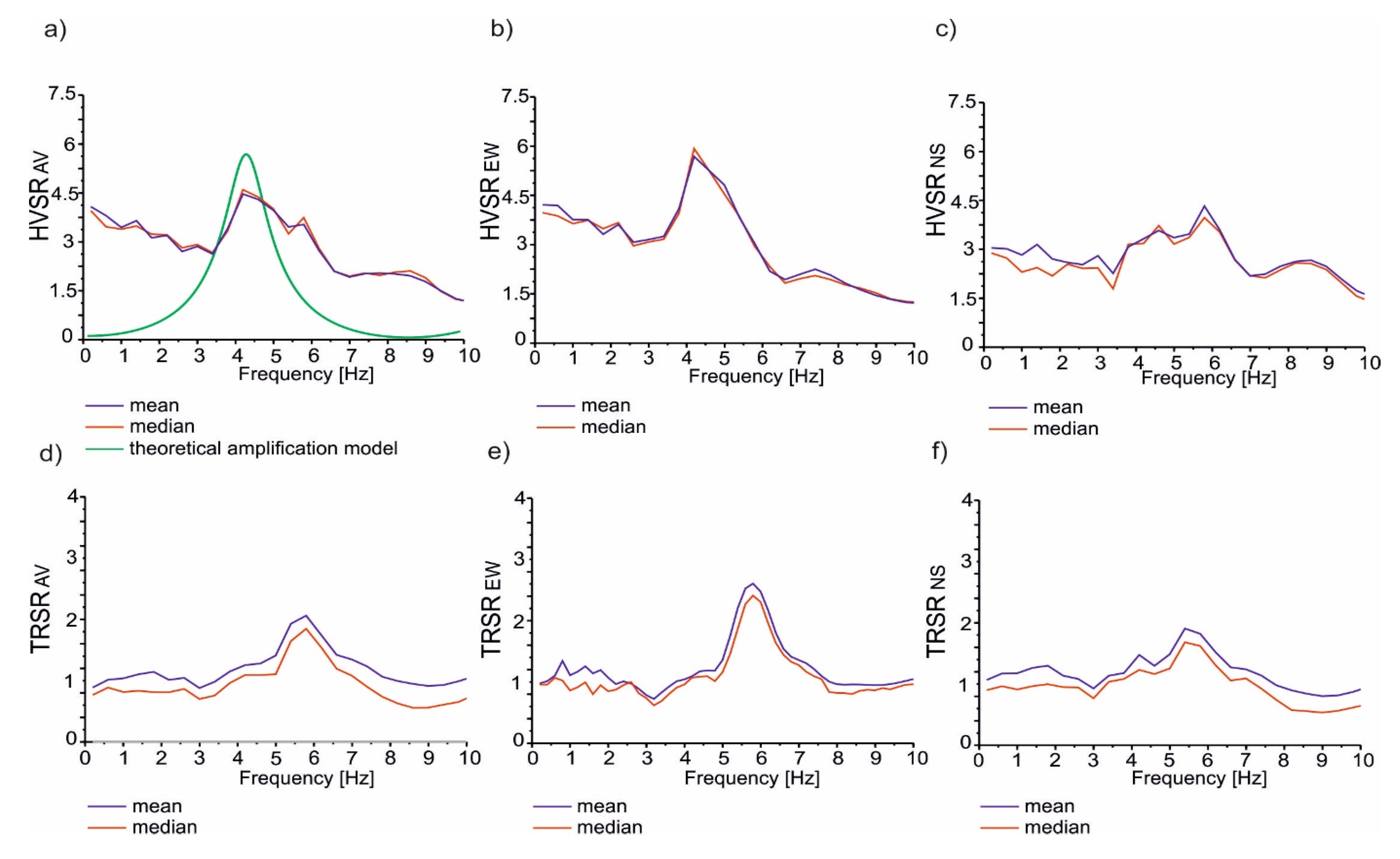
3.1. Site Effect Curves of the Translational and Rotational Motion

Based on the geological profiles (Figure 1d,f), the theoretical HVSR curves were estimated for the IMI and PLA stations as the first step of the analysis. The investigation of local geology allowed us to assess the two-layered geophysical models for both stations. The parameters required to estimate the theoretical HVSR curve are shown in

Table 2. Parameters of two-layered geophysical models and theoretical site effects.

Station	Vs Basement [m/s]	Vs Resonant [m/s]	Density Basement [g/cm3]	Density Resonant [g/cm3]	Attenuation Factor	Thickness [m]	Max (H/V)	f0 [Hz]
IMI	3800	400	2.5	1.8	0.05	62.0	6.4	1.65
PLA	2200	340	2.1	1.8	0.05	20.0	4.7	4.25

, containing values of the shear wave velocities (Vs), densities, attention coefficient, and the thickness of the resonant (soft) layer. The velocities in the resonant layer were found in the research performed in the same area [9], where the MASW technique was applied to recognize Vs30. For the IMI station, the Vs30 = 400 m/s value was used in the calculation. In the case of PLA, the average Vs value up to 20m was set as 340 m/s. The thickness of the resonant layer in the IMI station corresponded to the complex of loose Quaternary deposits and strongly weathered Triassic hydrocarbonates, which reached a thickness of over 60 m. The basement velocities were arbitrarily assumed [48], Table 2. The theoretical calculation of the site effects allowed us to estimate the amplification coefficients as 6.4 and 4.7 with corresponding resonance frequencies of 1.65 Hz and 4.25 Hz for the IMI and PLA stations, respectively.

The spectral ratios were estimated according to the SESAME criteria [35]. Each seismic record of 130 events was processed similarly. However, the difference between the process parameters was connected with the values of predicted resonance frequency and, therefore, the number of significant cycles, according to the SESAME criteria. As mentioned above, the number of significant cycles should exceed 200. Thus, in the case of the IMI station, the calculation was carried out under the assumption of the expected 1.65 Hz resonance frequency and windowing of the signals in a 5 s long time series (50 windows per signal). The calculation in the case of the PLA station was performed considering the expected 4.25 Hz resonance frequency and windowing the signals in a 3 s long time series (50 windows per signal). The empirical amplification and resonance frequency were found for average horizontal, EW, and NS directions. Subsequently, the arithmetic average was calculated from all events (Figure 4 and Figure 5). The ratio curves of the IMI station records allowed us to distinguish two general HVSR peaks and two TRSR peaks (

Table 3. Resonance frequencies and amplification factors were obtained for rotation and translation in each component: average, EW (x-axis), and NS (y-axis).

Type of Motion	Component	IMI Station				PLA Station
		Maximum I		Maximum II		Maximum
		f0 [Hz]	Amplification Peak Value	f0 [Hz]	Amplification Peak Value	f0 [Hz]	Amplification Peak Value
Translation	AV HVSR PGA	1.6	6.8	2.2	3.9	4.2	4.7
	EW PGA	1.6	6.7	2.4	3.4	5.8	4.3
	NS PGA	1.4	7.1	2.2	4.1	4.2	5.6
Rotation	AV TRSR PRV	1.8	2.5	4.4	1.6	5.6	1.9
	EW PRV	1.8	3.1	4.6	1.7	5.8	2.7
	NS PRV	1.8	3.7	4.4	1.7	5.4	1.8

). The first maximum was observed at frequencies ranging from 1.4 Hz to 1.6 Hz for translation and at 1.8 Hz for rotation. The second maximum of translation occurred at frequencies ranging from 2.2 Hz to 2.4 Hz, while for rotation, it ranged from 4.4 Hz to 4.6 Hz. The analysis of the PLA station records allowed to distinguish only one general HVSR peak and one TRSR peak (Table 3), observed at frequencies ranging from 4.2 Hz to 5.8 Hz for translation and 5.4 Hz to 5.8 Hz for rotation. Each of the spectral ratios for all 130 seismic events satisfied the first, second, and third rules concerning the criteria of reliable HVSR estimations. Consequently, according to the satisfied criteria of time-window length and the number of windows, dividing peak values of the seismic signals by the estimated amplification coefficient was allowed. Considering the HVSR and TRSR estimation results for the IMI station, we assumed that the first peak represented the central values of site effect parameters because it dominates over other H/V maxima observed on the curve. Considering the HVSR and TRSR estimation results for the IMI station, we assumed that the first peak represented the central values of site effect parameters because it dominates over other H/V maxima observed on the curve. In the case of the PLA station, only one maximum was generated, which allowed us to assume that it represents the main values of the local site effect coefficients. The recognized peaks of the TRSR and HVSR curves fulfilled the SESAME criteria, e.g., the ranges of the standard deviation of the resonant frequency.

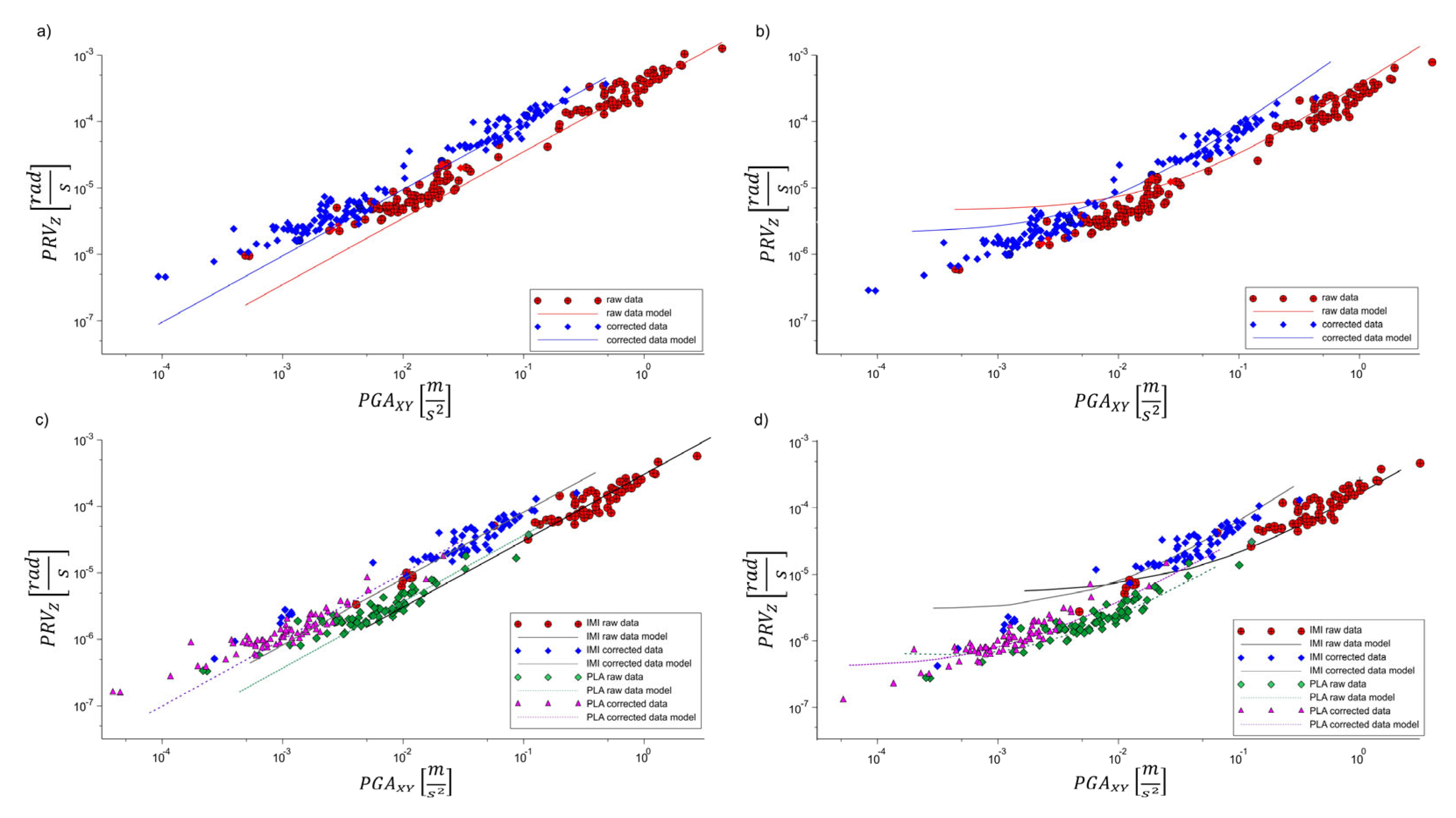
3.2. Peak Rotation and Translation Scaling Relations

The scaling relation for peak rotation and peak translation was analyzed for the set containing all data (IMI + PLA) and separated data sets (Figure 6). Moreover, two models were evaluated for each data set, i.e., linear function without intercept (Figure 6a,c) and linear function with intercept (Figure 6b,d). Statistical assessment was performed by applying the determination coefficient (R2) and the standard error of estimate (SEE). The fitting procedure was the orthogonal distance regression method. Assuming that the estimation of the HVSR and TRSR curves and peak values of the rotational and translational signals were found for the same type of body wave, the peak values were divided by the empirical amplification coefficients for the S-wave. Therefore, all calculations were conducted twice, first for the data sets with raw peak values and the second for data sets divided by the appropriate amplification coefficient.

The estimation results assuming the orthogonal distance regression method are shown in

Table 4. Regression results.

Station	Type of Data	Model Without Intercept			Model Intercept
		a ± Δa	R2	SEE	a ± Δa	B ± Δb	R2	SEE
Total	Raw data	(46.2 ± 0.6) × 10−5	0.93	1.6× 10−5	(40.7 ± 1.2) × 10−5	(5.1 ± 1.4) × 10−6	0.92	1.6 × 10−5
	Corrected data	(129.0 ± 1.3) × 10−5	0.93	5.5 × 10−6	(93.7 ± 2.1) × 10−5	(1.8 ± 0.4) × 10−6	0.93	5.7 × 10−6
IMI	Raw data	(45.4 ± 1.3) × 10−5	0.91	2.1× 10−5	(37.3 ± 1.4) × 10−5	(1.7 ± 0.6) × 10−6	0.89	2.3 × 10−5
	Corrected data	(100.8 ± 2.4) × 10−5	0.93	8.7 × 10−6	(87.4 ± 3.1) × 10−5	(5.4 ± 1.2) × 10−6	0.88	7.9 × 10−6
PLA	Raw data	(50.8 ± 1.5) × 10−5	0.92	1.8 × 10−6	(42.0 ± 1.9) × 10−5	(1.2 ± 0.5) × 10−6	0.89	1.6 × 10−6
	Corrected data	(129.0 ± 3.5) × 10−5	0.92	9.6× 10−7	(94.7 ± 3.8) × 10−5	(6.8 ± 1.2) × 10−6	0.89	8.6 × 10−7

. Twelve linear models were considered, and eight showed the determination coefficient R2 > 0.90. This simple parameter indicated that the linear models without an intercept generally fit better than those with an intercept b. Moreover, it is noticeable that the correction procedure produced higher values of slope a than the raw data points in each case. In the case of the entire model, the slope increased from 4.07 × 10⁻⁴ to 9.37 × 10⁻⁴, while for the model without the intercept, the values changed from 4.62 × 10⁻⁴ to 1.29 × 10⁻³. An opposite situation can be noticed for the b-parameter, which decreased from 5.1 × 10⁻⁶ to 1.79 × 10⁻⁶ after data correction. The separate models for the IMI and PLA stations presented similar behavior. In the case of the IMI station, the correction caused an increase in a-parameter from 4.54 × 10⁻⁴ to 1.00 × 10⁻³. The same parameters for the PLA station increased from 5.08 × 10⁻⁴ to 1.29 × 10⁻³. Nevertheless, taking into account the model with the intercept for the IMI station, the correction procedure caused an increase in both regression parameters—from 3.73 × 10⁻⁴ to 8.74 × 10⁻³ for the slope and from 1.70 × 10⁻⁶ to 5.40 × 10⁻⁶ for the intercept. In the case of the PLA station, the regression parameters change their values from 4.20 × 10⁻⁴ to 9.47 × 10⁻⁴ and from 1.20 × 10⁻⁶ to 6.80 × 10⁻⁶ for the slope and intercept, respectively.

4. Discussion

4.1. Site Effect Differences

Comparing the results for the HVSR and TRSR estimations, it can be noticed that the resonance frequencies were differential, and the rotational resonance frequencies were higher than translational. In the case of the IMI station, the resonance frequencies corresponding to the first maximum of the average H/V ratio reached 1.6 Hz and 1.8 Hz (Table 3) for translation and rotation, respectively. The PLA station also showed higher values of the rotational resonance frequency (for average H/V) of 5.6 Hz than the translational resonance frequency of 4.2 Hz (Table 3). Similar differences were observed for the EW and NS directions (Table 3). A question arises as to what influences the change in the resonance frequency. The resonance frequency can be approximated as follows [40]:

$$f_0={\displaystyle \frac{V_s}{4H}}$$

(13)

where $V_S$ is the shear wave velocity, H is the thickness, and $f_0$ denotes the resonance frequency. Considering the dependence on rotational resonance frequency similar to the translational motion, the rotational records were probably influenced by the amplification effect produced by shallow structures according to Equation (13). The difference in the resonance frequency for the IMI station is insignificant. Thus, the thickness of the resonance layer is similar for both types of motion. Nevertheless, the result from the PLA station showed a shift between the resonance frequencies, which can be related to the varied values of H (Equation (13)). Taking into account that both sensors were mounted directly in the same place and geological settings were unchanged, other factors might affect the resonance shift. As mentioned before, in the case of the PLA station, the 20 m thick resonance layer corresponded to the shallow Quaternary sediments (up to 5 m thick) and strongly weathered Carboniferous layer, mainly eroded or fractured. One of the factors that might affect the resonance frequency shift was related to the intense fractures occurring in the shallow layers. The geological structures were less compacted in the PLA station than in the IMI station, which could have caused the higher value of the rotational resonance frequency for the lower H-value (Figure 7) [22,24].

Moreover, a detailed observation indicated the presence of a water body table at a depth of ca. 15 m below the surface. A simple assessment of the H-value for the rotation resonance effect showed that the resonance layer corresponded to the water table depth (Figure 7). Therefore, in the case of the PLA station, the water body did not influence the translational resonance effect but might have changed the nature of the rotational resonance. An in-depth investigation should be carried out to determine which factors (fractures, water bodies, or both) had a tangible impact on the rotational resonance frequency. Detailed surveys about the impact of local small-scale heterogeneities on the rotational motion [49] confirm the explanations presented above. The occurrence of the geological heterogeneities had a real effect on the wavefield gradient measurements: strain and rotation. In contrast, the impact of heterogeneities may be insignificant in the wavefield measurements (i.e., translational acceleration). The effect of the heterogeneities on the rotations can be caused by altering the phase and amplitude of the signal, whose intensity depends mainly on the velocity contrast but not on the spatial extent of the heterogeneities. Therefore, considering the results obtained for the resonance frequency for the IMI station and PLA station, it can be concluded that geological discontinuities change the nature of the rotational motion compared to the translational motion. Consequently, different geological layers can produce the rotational site effect and not the translational. The rotation amplification coefficients for the IMI and PLA stations were more than two times lower than those of the respective translational ones. As was mentioned above, the predictive models of the rotational amplification for the specific geological setting are unknown, and their relation to the translational site effect parameters is unknown. Therefore, at this moment, the presented observation cannot be treated as a constant and stable tendency for the rotational motion. Because translational amplification value depends on the arrangements of specific geological structures, their influence on the rotations might have occurred similarly. Nevertheless, some questions arose during this study: (a) Is the rotational amplification coefficient consistently lower than the corresponding translational one, or in some specific cases, is this trend opposite? (b) Can the translational and rotational site effect parameter relation be expressed with a mathematical function? Regarding the answer to the first question, some researchers [21] presented that the rotational H/V ratio was higher than the respective translational one. This leads to the conclusion that the local site conditions independently affect the rotational and translational motions, and therefore, the tendency to obtain a lower value of the amplification by rotational motion cannot be treated as constant. Thus, answering the second question, the potential mathematical expression between the rotational and translational site effect parameters probably does not exist because geological conditions affect the rotational and translational motions differently. Considering the parameters used in the H/V estimations, it is tough to ignore that the time window length (except in the case of the IMI station) should encompass the S-wave phase and the Rayleigh waves. However, the data sets from the IMI station exclude the presence of the Rayleigh waves on the 54 registered signals due to the meager epicentral distance. Considering that the analyzed seismic events were characterized by a double-couple source mechanism, the S-wave phase is dominant on the records. The minimum distance of the Rayleigh wave generation is given by the following formula [50]:

$$s_s={\displaystyle \frac{V_r}{\sqrt{{\beta }^2-{Vr}^2}}}d$$

(14)

where $V_R$ is the Rayleigh wave velocity (which is equal to 0.9$\beta$), $\beta$ is the shear wave velocity, and d denotes the depth of the event source.

The depth of the events ranged from 1.0 km to 1.2 km, and the shear wave velocity of the surface layer was 2080 m/s, which caused the minimal distance of Rayleigh wave generation to range from 2.0 km to 2.4 km. Epicentral distances up to 2.0 km characterized the 54 analyzed events from the IMI station. The epicentral distance for the rest of the events was 4.0 km to 5.5 km. Consequently, the possibility of encompassing the Rayleigh wave in H/V spectrum analysis is significant. However, the influence of those events on the estimated H/V spectrum (Figure 4) was negligible. In the case of the PLA station, the epicentral distance did not exclude the presence of the Rayleigh wave on the signals, but time widow length should not encompass the S-wave phase and the Rayleigh waves. Nevertheless, regarding the type of data recorded by the IMI and PLA stations, one is obligated to pay attention to aspects connected with the SESAME criteria and definition of the cycle numbers, except in terms of the time window length. Considering the SESAME criteria, the time window length should be fulfilled in the following criteria:

$$f_0>{\displaystyle \frac{10}{l_w}}$$

(15)

where $l_w$ is the window length and $f_0$ denotes resonance frequency.

Considering the data character of the IMI station, in the case of events from a longer distance than analyzed, the time window length of about 5s will encompass the surface waves. A similar situation occurs when the registered event is less distant at the PLA station—in that case, reducing the time window value and increasing the time window history. The natural consequence of that situation is the unfulfillment of the reliability criteria of the H/V curve from equation 15. In that situation, the estimation of the H/V spectrum of the registered microtremors may be treated as additional surveys, which can confirm the reliability of the spectrum obtained from the body wave analysis. Alternatively, the estimation process of the H/V spectrum of the rotational and translational motion can be carried out by using a response spectrum instead of the Fourier transform method [22,23]. The obtained peak can be used to determine the global resonance peak in the case of multiple peaks on the spectrum. Nevertheless, the limitation of the response spectrum method is the tendency of the scenario dependence (i.e., magnitude, distance, focal mechanism, etc.) of the events [22,23]. In the case of TRSR estimation by using the response spectrum method, the applicability of that method is strongly related to the dimension of the document where the sensors were deployed; increasing the dimension caused damping of the torsion component and, thus, sequence inability of the H/V estimation [23]. Nevertheless, as was mentioned above, the HVSR estimation, despite the aspect of the amplification curve reliability, may produce a spectrum in which the recognition of the general amplification is problematic due to the occurrence of a broad peak or unclear low amplification peak. Origin of that kind of spectrum is often related to lousy soil-sensor coupling, especially on wet soils or grass, low-frequency sites with either moderate impedance contrast at depth, occurrence of meteorological perturbation, wrongly chosen smoothing parameters, or short distance to the artificial ambient vibration sources, such as public work machines or trucks. In contrast, multiple amplification peaks in most cases are related to industrial origin (machinery occurrence) but, in many instances, may be associated with the local geology and strong fracturing occurrence [51,52]. In that case, geological conditions had to be diagnosed and supported by additive geophysical research, such as MASW or resistivity methods, to find the physical properties.

Finally, we may summarize the above-mentioned discussion as follows:

1. The occurrence of the local small-scale heterogeneities had an impact on the rotational motion and is relatively responsible for the resonance frequency shift noted at the PLA station.

2. A comparison of the results from the PLA and IMI stations suggests that different geological layers can produce the rotational site effect rather than the translational.

3. Lower values of the rotational amplification in comparison to the translations cannot be treated as a constant.

4. The local site conditions independently affect the rotational and translational motions.

4.2. Scaling Relation

The tested linear models, with and without the intercept, showed a perfect fit assessment with R2 > 0.85 and low values of SEE < 2.5 × 10⁻⁵. However, the models without the intercept provided the highest R2 values. This suggests that the model of PRV = aPGA seems to be more accurate than the model with intercept. Nevertheless, the analysis showed that all obtained models are reliable. According to previous research [11], the Vs30 significantly influences the regression parameters; however, the models (for IMI and PLA station) obtained for the raw data seem to be convergent, and comparable Vs30 values cause this similarity in both cases. So far, the presented scaling relations have not considered the amplification phenomenon in the near-surface layer. The scaling relations in the recent studies [4,5,11,26,45] were performed for the natural events registered in a greater epicentral distance than in the case of our study. Therefore, it is tough to ignore the possibility that the peak values were registered at the group of the surface waves, while in the case of our study, they were registered at the S-wave part. Therefore, the a coefficient should be considered as a slowness of the S-wave, while in the case of the recent studies [4,5,11,26,45], the a coefficient is connected with the slowness of the Love waves and denoted as the c. Therefore, the models presented in our study should be treated separately due to differences in estimating the scaling relation for the peak values registered at the group of the surface waves. Nevertheless, the primary issue is still connected with the site effect impact on the determined scaling relations. In the presented study, the estimated peak values of the H/V ratio were used to correct the peak values of the signals and, consequently, remove the site effect impact on the estimated scaling relation. Moreover, the peak values of the signals were divided by the single amplification value, which was allowed due to the generation of the single clear peak of the amplification on the H/V spectrum. In the case of multiple amplification peaks on the H/V spectrum, this procedure should be changed to dividing signal peak values respective to that event H/V spectrum. The designation of the general peak of the H/V ratio in case of multiple peak occurrences can be done by estimating the H/V ratio using the response spectrum method, which should present one general peak [43]. Taking into account the research carried out for the same database [22,23], the H/V ratio obtained from the response spectrum method presented identical general peaks for the same database, as was given during that research. Therefore, the obtained general peak values of the H/V ratio can be used to reduce the impact of amplification on the signal peak values. The new models converge (Figure 8), confirming their universal application for the USCB area. If they were different, something else would influence their trend apart from amplification and local geological conditions.

The other worldwide models presented in Figure 8 differ from models from this study, which is an effect of the studied scaling relation for the signal peak values obtained for the surface waves. The presented scaling relations are based on two linear models: with and without the intercept. The function without the intercept has an explanation resulting from Equation (4). Nevertheless, some authors [5,26,45] used the function with the intercept b. The physical nature of the parameter is unknown; it is only mathematical. The calculated b-values were low and can be assumed to be negligible. However, the non-zero b-value suggests that the rotation peak can exist without a translation motion. Forcing the b-value to 0 improved the statistical fit of the observational data to the model and increased the slope, resulting in an insignificant a-value modification. Using the function with intercept b also has another limitation. As Figure 6b shows, fitting raw and corrected data can create some estimation problems. The reason for this can be that one of the sensors was rotated by several degrees during the observation, and its registrations were disturbed by a deviation from the main geographic direction. However, errors of this type should affect the total recorded data. Thus, we can assume that a better fit would be obtained in terms of another estimation mode, which will depend on the exact ranges of recorded values—rotational or translational. Still, it cannot be taken for granted that one estimated model can be applied to all registration ranges. Based on recent research [21], in the case of the scaling relation between the vertical PRV and horizontal PGV, the function’s slope is linked to the complexity of the local geology. The more excellent slope value should produce a higher value of the PRV for a given PGA of vertical component and, therefore, describe a more complicated surface geology [53]. Thus, considering our research, the potential connection of the a parameter with the complexity of the local geology cannot be excluded. Recent studies [5,11,26,45] connected the a parameter with the local surface geology. Considering that the presented scaling relation was obtained for the peak values of the S-wave signal part, a should be linked to the apparent SH wave phase velocity [21]. Considering similar studies [21], the estimated apparent SH-wave phase velocity c equaled 379 m/s, with a standard deviation of 114 m/s. In the case of our study, a is proportional to 1/(2c). Considering the results obtained for directly registered peak values and the model without intercept, the SH-wave phase velocity for the IMI and PLA stations was 1101 m/s and 982 m/s, respectively. However, the correction by an amplification value caused the SH-wave phase velocity for the IMI and PLA stations to reach 496 m/s and 387 m/s, respectively. The analyzed total models (Figure 5a,b) showed regression parameters similar to those for the separate IMI and PLA data. The question is whether these total models are universal. The location of the stations suggested similar geotechnical conditions due to the similar Vs30 value. Therefore, the obtained total models were expected to be a good approximation and match the empirical data. However, detailed visual inspection revealed that the model did not intersect the center of the points but generally emphasized points on the periphery. Therefore, the presented total model, obtained for two data sets with similar Vs30, cannot be treated as one model.

The above discussion can be summarized as follows:

1. Correction of the data set by measured amplification value increases the approximation of the scaling relation model to the data by removing the local site effect from the data.

2. The scaling relation model without an intercept better approximated the data.

3. Correction by the amplification resulted in a lowered value of the apparent SH-wave and suggested a correlation of the function slope to the complexity of the local geology.

5. Conclusions

The presented study estimated the site effect parameters for rotational and translational motions registered at two separate stations. For the IMI station, the resonance frequencies of translational and rotational motions were almost the same, which indicates that the resonance effect occurred in the same near-surface rock volume. On the other hand, in the case of the PLA station, a significant difference between the resonance frequencies was observed, which suggested different depth levels of the resonance layer. The rotational resonance effect probably occurred in the shallower volume of rock than translational due to intense fractures and the water table. These geological factors affect the depth range of the rotational motion (Figure 7). The two studied stations were independent; however, by coincidence, they were characterized with similar Vs30 parameters. This similarity influenced the final result of the total model comparison, and the comparison of single-site models produced the a-parameter values close to each other. However, these similarities cannot be taken for granted. The correction of the scaling relation showed that amplification effects influenced the scaling relation model by changing the SH wave phase velocity value.

References

1. Zembaty, Z. Deriving seismic surface rotations for engineering purposes. In Earthquake Source Asymmetry, Structural Media and Rotation Effects; Teisseyre, R., Majewski, E., Takeo, M., Eds.; Springer: Berlin/Heidelberg, Germany, 2006; pp. 549–568. [Google Scholar]
2. Igel, H.; Cochard, A.; Wassermann, J.; Schreiber, U.; Velikoseltsev, A.; Pham, N.D. Broadband observations of rotational ground motions. Geophys. J. Int. 2007, 168, 182–197. [Google Scholar] [CrossRef]
3. Lee, V.W.; Liang, L. Rotational components of strong motion earthquakes. In Proceedings of the 14th World Conference on Earthquake Engineering, Beijing, China, 12–17 October 2008. [Google Scholar]
4. Lee, W.H.K.; Huang, B.S.; Langston, C.A.; Lin, C.J.; Liu, C.C.; Shin, T.C.; Teng, T.L.; Wu, C.F. Review: Progress in rotational ground motion observations from explosions and local earthquakes in Taiwan. Bull. Seismol. Soc. Am. 2009, 99, 958–967. [Google Scholar] [CrossRef]
5. Liu, C.C.; Huang, B.S.; Lee, W.H.K.; Lin, C.J. Observing rotational and translational ground motions at the HGSD station in Taiwan from 2007 to 2008. Bull. Seismol. Soc. Am. 2009, 99, 1228–1236. [Google Scholar] [CrossRef]
6. Stupazzini, M.; de la Puente, J.; Smerzini, C.; Käser, M.; Igel, H.; Castellani, A. Study of Rotational Ground Motion in the Near-Field Region. Bull. Seismol. Soc. Am. 2009, 99, 1271–1286. [Google Scholar] [CrossRef]
7. Kalab, Z.; Knejzlik, J.; Lednicka, M. Application of newly developed rotational sensor for monitoring of mining-induced seismic events in the Karvina region. Acta Geodyn. Geomater. 2012, 2, 197–205. [Google Scholar] [CrossRef]
8. Zembaty, Z.; Mutke, G.; Nawrocki, D.; Bobra, P. Rotational ground-motion records from induced seismic events. Seismol. Res. Lett. 2017, 88, 13–22. [Google Scholar] [CrossRef]
9. Mutke, G.; Lurka, A.; Zembaty, Z. Prediction of rotational ground motion for mining-induced seismicity—Case study from Upper Silesian Coal Basin, Poland. Eng. Geol. 2020, 276, 105767. [Google Scholar] [CrossRef]
10. Sarokolayi, L.K.; Beitollahi, A.; Abdollahzadeh, G.; Amreie, S.T.T.; Kutanaei, S.S. Modeling of ground motion rotational components for near-fault and far-fault earthquake according to soil type. Arab. J. Geosci. 2015, 8, 3785–3797. [Google Scholar] [CrossRef]
11. Sbaa, S.; Hollender, F.; Perron, V.; Imtiaz, A.; Bard, P.-Y.; Mariscal, A.; Cochard, A.; Dujardin, A. Analysis of rotation sensor data from the SINAPS@ Kefalonia (Greece) post-seismic experiment—Link to surface geology and wavefield characteristics. Earth Planets Space 2017, 69, 124. [Google Scholar] [CrossRef]
12. Wang, H.; Igel, H.; Gallovič, F.; Cochard, A. Source and Basin Effects on Rotational Ground Motions: Comparison with Translations. Bull. Seismol. Soc. Am. 2009, 99, 1162–1173. [Google Scholar] [CrossRef]
13. Pham, N.D.; Igel, H.; Puente, J.; Käser, M.; Schoenberg, M. Rotational motions in homogeneous anisotropic elastic media. Geophysics 2010, 75, 47–56. [Google Scholar] [CrossRef]
14. Trifunac, M.D. The role of strong motion rotations in the response of structures near earthquake faults. Soil Dyn. Earthq. Eng. 2009, 29, 382–393. [Google Scholar] [CrossRef]
15. Basu, D.; Whittaker, A.S.; Constantinou, M.C. Characterizing rotational components of earthquake ground motion using a surface distribution method and response of sample structures. J. Eng. Struct. 2015, 99, 685–707. [Google Scholar] [CrossRef]
16. Falamarz-Sheikhabadi, M.R.; Ghafory-Ashtiany, M. Rotational components in structural loading. Soil Dyn. Earthq. Eng. 2015, 75, 220–233. [Google Scholar] [CrossRef]
17. Bońkowski, P.A.; Zembaty, Z.; Minch, M.Y. Engineering analysis of strong ground rocking and its effect on tall structures. Soil Dyn. Earthq. Eng. 2019, 116, 358–370. [Google Scholar] [CrossRef]
18. Huang, M.; Fan, X.; Wang, H. Three-dimensional upper bound stability analysis of slopes with weak interlayer based on rotational-translational mechanisms. Eng. Geol. 2017, 223, 82–91. [Google Scholar] [CrossRef]
19. Jiren, X.; Uchimura, T.; Wang, G.; Selvarajah, H.; Maqsood, Z.; Shen, Q.; Mei, G.; Qiao, S. Predicting the sliding behaviour of rotational landslides based on the tilting measurement of the slope surface. Eng. Geol. 2020, 269, 105554. [Google Scholar] [CrossRef]
20. Nakamura, Y. A method for dynamic characteristics estimation of subsurface using microtremor on the ground surface. Q. Rep. RTRI 1989, 130, 25–33. [Google Scholar]
21. Ringler, A.; Anthony, R.; Holland, A.; Wilson, D.; Lin, C.J. Observations of Rotational Motions from Local Earthquakes Using Two Temporary Portable Sensors in Waynoka, Oklahoma. Bull. Seismol. Soc. Am. 2018, 108, 3562–3575. [Google Scholar] [CrossRef]
22. Nawrocki, D.; Mendecki, M.; Teper, L. Estimation of site resonance frequency using HVSR method for rotational and translational signals: Result comparison from Fourier and response spectrum methods. In Proceedings of the 3rd European Conference on Earthquake Engineering and Seismology, Bucharest, Romania, 4–9 September 2022. [Google Scholar]
23. Nawrocki, D.; Mendecki, M.; Teper, L. Estimation of the resonance frequency of rotational and translational signals evoked by mining-induced seismicity. Front. Earth Sci. 2024, 12, 1403043. [Google Scholar] [CrossRef]
24. Nawrocki, D.; Mendecki, M.; Teper, L. The effects of component rotation on H/V spectra: A comparison of rotational and translational data. Geol. Geophys. Environ. 2024, 50, 145–154. [Google Scholar]
25. Igel, H.; Schreiber, U.; Flaws, A.; Schuberth, B.; Velikoseltsev, A.; Cochard, A. Rotational motions induced by the M8.1 Tokachi-oki earthquake, September 25, 2003. Geophys. Res. Lett. 2005, 32, L08309. [Google Scholar] [CrossRef]
26. Takeo, M. Rotational motions observed during an earthquake swarm in April 1998 offshore Ito, Japan. Bull. Seismol. Soc. Am. 2009, 99, 1457–1467. [Google Scholar] [CrossRef]
27. Sagan, G.; Teper, L.; Zuberek, W.M. Tectonic analysis of mine tremor mechanisms from the Upper Silesian Coal Basin. Pure Appl. Geophys. 1996, 147, 217–238. [Google Scholar] [CrossRef]
28. Buła, Z.; Kotas, A. (Eds.) Geological Atlas of the Upper Silesian Coal Basin, Part III. Structural-Geological Maps 1:100 000; Państwowy Instytut Geologiczny: Warszawa, Poland, 1994. [Google Scholar]
29. Teper, L. Geometry of fold arrays in the Silesian-Cracovian region of southern Poland. Geol. Soc. Spec. Publ. Lond. 2000, 169, 167–179. [Google Scholar] [CrossRef]
30. Mendecki, M.J.; Szczygieł, J.; Lizurek, G.; Teper, L. Mining-triggered seismicity governed by a fold hinge zone: The Upper Silesian Coal Basin, Poland. Eng. Geol. 2020, 274, 105728. [Google Scholar] [CrossRef]
31. Jureczka, J.; Aust, J.; Buła, Z.; Dopita, M.; Zdanowski, A. Geological Map of the Upper Silesian Coal Basin (Carboniferous Subcrop) 1:200 000; Państwowy Instytut Geologiczny: Warszawa, Poland, 1995. [Google Scholar]
32. Stec, K. Characteristics of seismic activity of the Upper Silesian Coal Basin in Poland. Geophys. J. Int. 2006, 168, 757–768. [Google Scholar] [CrossRef]
33. eentec. Instruction Manual, Model R-1, St. Louis, Missouri. 2008. 8p. Available online: http://www.eentec.com/ (accessed on 1 July 2020).
34. Bernauer, F.; Wassermann, J.; Igel, H. Rotational sensors—A comparison of different sensor types. J. Seismol. 2012, 16, 595–602. [Google Scholar] [CrossRef]
35. Mutke, G.; Kotyrba, A.; Lurka, A.; Olszewska, D.; Dykowski, P.; Borkowski, A.; Araszkiewicz, A.; Barański, A. Upper Silesian Geophysical Observation System—A unit of the EPOS project. J. Sustain. Min. 2019, 18, 198–207. [Google Scholar] [CrossRef]
36. Bard, P.Y.; SESAME Participants. The SESAME project: An overview and main results. In Proceedings of the 13th World Conference on Earthquake Engineering, Paper 2207, Vancouver, BC, Canada, 1–6 August 2004. [Google Scholar]
37. Stephenson, W.J.; Hartzell, S.; Frankel, A.; Asten, M.; Carver, D.; Kim, W. Site characterization for urban seismic hazards in lower Manhattan, New York City, from microtremor array analysis. Geophys. Res. Lett. 2009, 36, L03301. [Google Scholar] [CrossRef]
38. Pastén, C.; Sáez, M.; Ruiz, S.; Leyton, F.; Salomón, J.; Poli, P. Deep Characterization of the Santiago Basin using HVSR and Cross-correlation of Ambient Seismic Noise. Eng. Geol. 2015, 201, 57–66. [Google Scholar] [CrossRef]
39. Stanko, D.; Markušić, S.; Strelec, S.; Gazdek, M. HVSR analysis of seismic site effects and soil-structure resonance in Varaždin city (North Croatia). Soil. Dynam Earthq. Eng. 2017, 92, 666–677. [Google Scholar] [CrossRef]
40. Stanko, D.; Markušić, S. An empirical relationship between resonance frequency, bedrock depth and VS30 for Croatia based on HVSR forward modelling. Nat. Hazards 2020, 103, 3715–3743. [Google Scholar] [CrossRef]
41. Szczygieł, J.; Wróblewski, W.; Mendecki, M.J.; Hercman, H.; Bosák, P. Soft-sediment deformation structures in cave deposits and their possible causes (Kalacka Cave, Tatra Mts., Poland). J. Struct. Geol. 2020, 140, 104161. [Google Scholar] [CrossRef]
42. Kawase, H. Site effects on strong ground motions. In International Handbook of Earthquake and Engineering Seismology; Lee, W.H., Jennings, P., Kisslinger, C., Kanamori, H., Eds.; 81B; Academic Press: Cambridge, MA, USA, 2002; pp. 1013–1030. [Google Scholar]
43. Rong, M.; Fu, L.Y.; Wang, Z.; Li, X.; Carpenter, N.S.; Woolery, E.W.; Lyu, Y. On the amplitude discrepancy of HVSR and site amplification from strong-motion observations. Bull. Seismol. Soc. Am. 2017, 107, 2873–2884. [Google Scholar] [CrossRef]
44. Zhu, C.; Cotton, F.; Pilz, M. Detecting Site Resonant Frequency Using HVSR: Fourier versus Response Spectrum and the First versus the Highest Peak Frequency. Bull. Seismol. Soc. Am. 2020, 110, 427–440. [Google Scholar] [CrossRef]
45. Yin, J.; Nigbor, R.L.; Chen, Q.; Steidl, J. Engineering analysis of measured rotational ground motions at GVDA. Soil. Dyn. Earthq. Eng. 2016, 87, 125–137. [Google Scholar] [CrossRef]
46. Konno, K.; Ohmachi, T. Ground-Motion Characteristics Estimated from Spectral Ratio between Horizontal and Vertical Components of Microtremor. Bull. Seismol. Soc. Am. 1998, 88, 228–241. [Google Scholar] [CrossRef]
47. Suryanto, W. Rotational Motions in Seismology: Theory and Application. Ph.D. Dissertation, Ludwig-Maximilians University München, Faculty of Geosciences, München, Germany, 2006. [Google Scholar]
48. Schön, J. Physical Properties of Rocks: A Workbook; Elsevier: Oxford, UK, 2011; Volume 8. [Google Scholar]
49. Singh, S.; Capdeville, Y.; Igel, H. Correcting wavefield gradients for the effects of local small-scale heterogeneities. Geophys. J. Int. 2020, 220, 996–1011. [Google Scholar] [CrossRef]
50. Okamoto, S. Introduction to Earthquake Engineering; University of Tokyo Press: Tokyo, Japan, 1984. [Google Scholar]
51. Pischiutta, M.; Rovelli, A.; Salvini, F.; Fletcher, J.B.; Savage, M.K. Directional Amplification at Rock Sites in Fault Damage Zones. Appl. Sci. 2023, 13, 6060. [Google Scholar] [CrossRef]
52. Pischiutta, M.; Savage, M.K.; Holt, R.A.; Salvini, F. Fracture-related wavefield polarization and seismic anisotropy across the Greendale Fault. J. Geophys. Res. Solid Earth 2015, 120, 7048–7067. [Google Scholar] [CrossRef]
53. Moriya, T.; Teisseyre, R. Design of rotation seismometer and non-linear behavior of rotation components of earthquakes. In Earthquake Source Asymmetry, Structural Media and Rotation Effects; Teisseyre, R., Majewski, E., Takeo, M., Eds.; Springer: Berlin/Heidelberg, Germany, 2006; pp. 439–450. [Google Scholar]
Figure 1. Study site information: (a) Investigation area on the map of Poland; (b) Sketch of USCB with study site location (modified after [28]); (c) Map of the study site with seismic event distribution and IMI station locations; (d) Generalized geological profile of the IMI station site; (e) Map of the study site with seismic event distribution and PLA station locations; (f) Generalized geological profile of the PLA station site.
Applsci 15 00102 g001
Figure 2. Seismogram of the seismic event: (a) Registered at the PLA station on 3 June 2016, the local magnitude reached 3.5, and the epicentral distance was equal to 9.7 km; (b) Registered at the IMI station on 9 June 2017, the local magnitude reached 2.1, and the epicentral distance was equal to 1.3 km.
Applsci 15 00102 g002
Figure 3. Motion directions in: (a) translation and (b) rotation, and (c) an ideal sketch of amplification effect in a soft layer.
Applsci 15 00102 g003
Figure 4. HVSR and TRSR curves of 60 events from the IMI station: (a) Average HVSR for translational acceleration and theoretical amplification model (green line); (b) HVSR in EW direction for translational acceleration; (c) HVSR in NS direction for translational acceleration; (d) Average TRSR rotational velocity; (e) TRSR in EW direction for rotational velocity; (f) TRSR in NS direction for rotational velocity.
Applsci 15 00102 g004
Figure 5. HVSR and TRSR curves of 70 events from the PLA station: (a) Average HVSR for translational acceleration and theoretical amplification model (green line); (b) HVSR in EW direction for translational acceleration; (c) HVSR in NS direction for translational acceleration; (d) Average TRSR rotational velocity; (e) TRSR in EW direction for rotational velocity; (f) TRSR in NS direction for rotational velocity.
Applsci 15 00102 g005
Figure 6. Peak rotation scaling relations for the raw and corrected data: (a) Assuming both station records as one model without intercept; (b) Assuming both station records as one model with intercept; (c) Separation models for the IMI and PLA station without intercept; (d) Separation models for the IMI and PLA station with intercept.
Applsci 15 00102 g006
Figure 7. Models of translation and rotation resonance effects with amplified horizontal amplitudes in near-surface and different depth ranges [22,24].
Applsci 15 00102 g007
Figure 8. Comparison of the scaling relation models between peak values of the rotational velocity and translational acceleration [5,26,45].
Applsci 15 00102 g008