
Prediction of GNSS Velocity Accuracies Using Machine Learning Algorithms for Active Fault Slip Rate Determination and Earthquake Hazard Assessment

Abstract
:1. Introduction
2. Materials and Methods
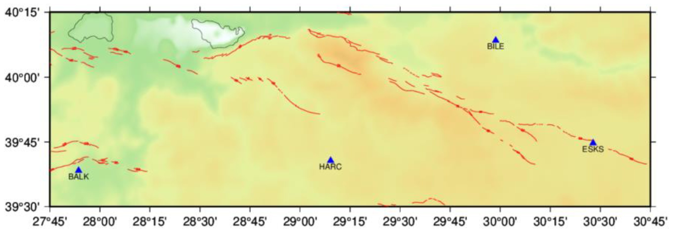
2.1. Preparation of the Dataset
2.2. Machine Learning
2.2.1. Multiple Linear Regression
2.2.2. Support Vector Machines
2.2.3. Random Forest
2.2.4. K-Nearest Neighbor Regression (KNN)
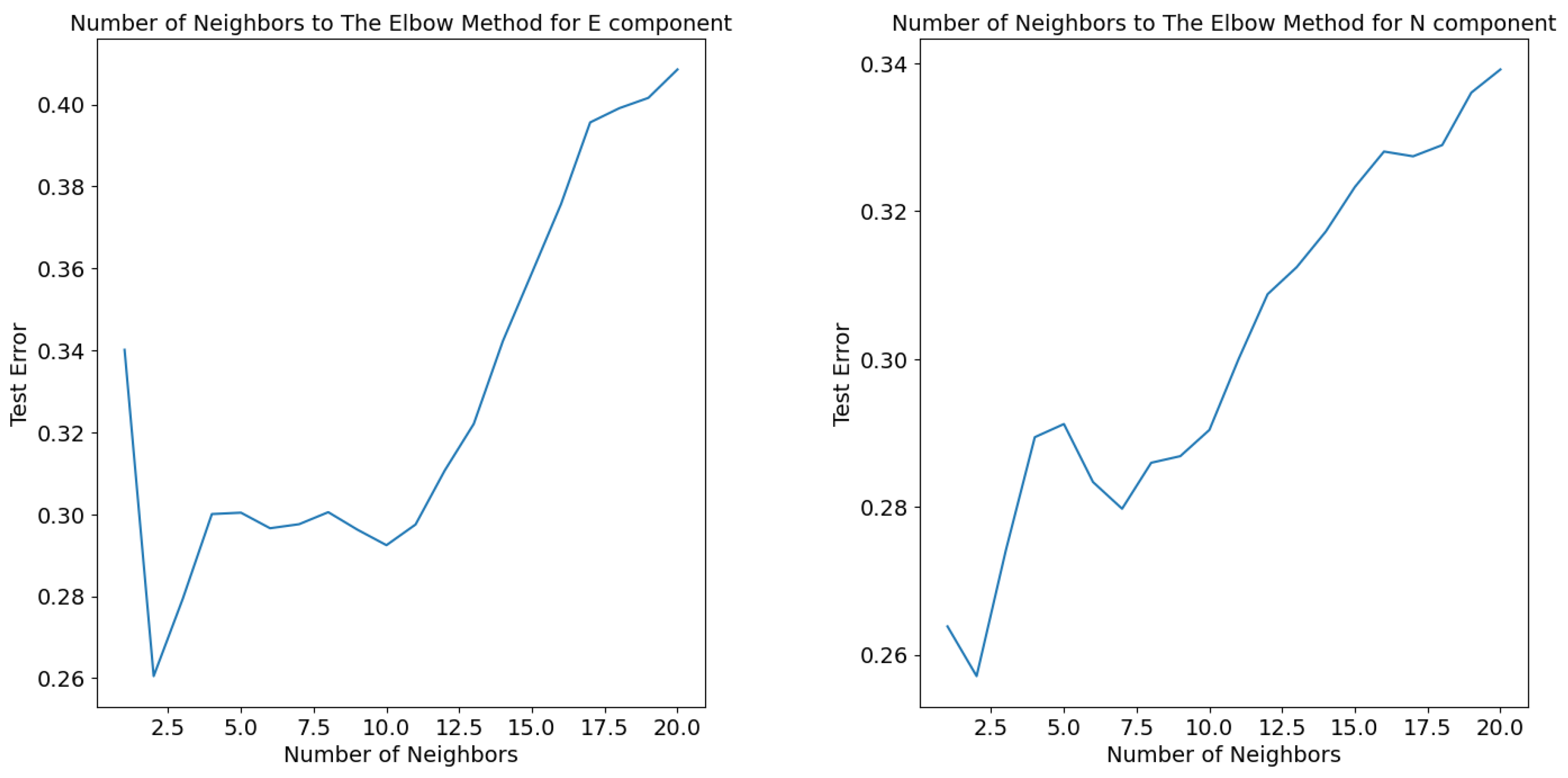
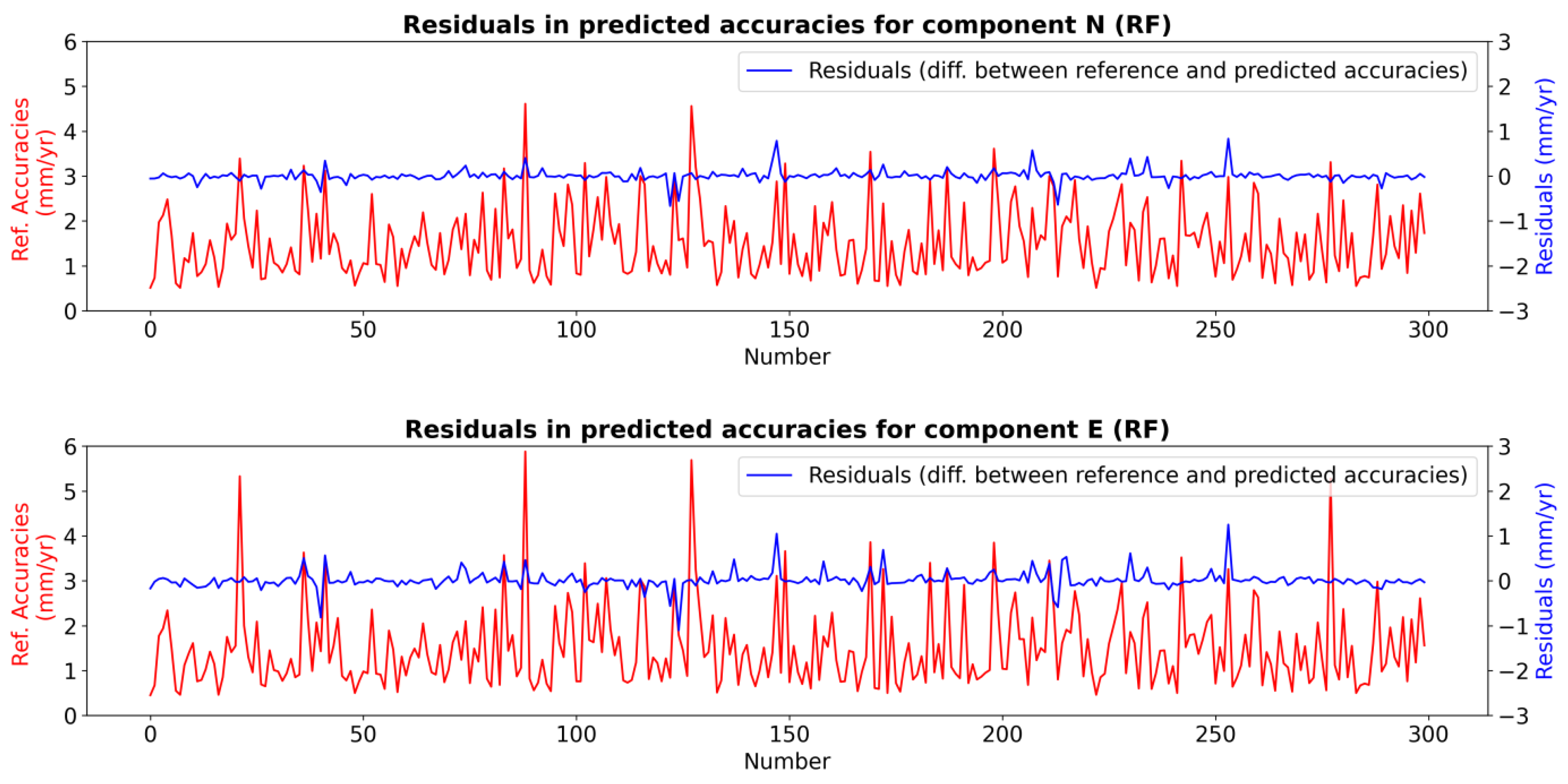
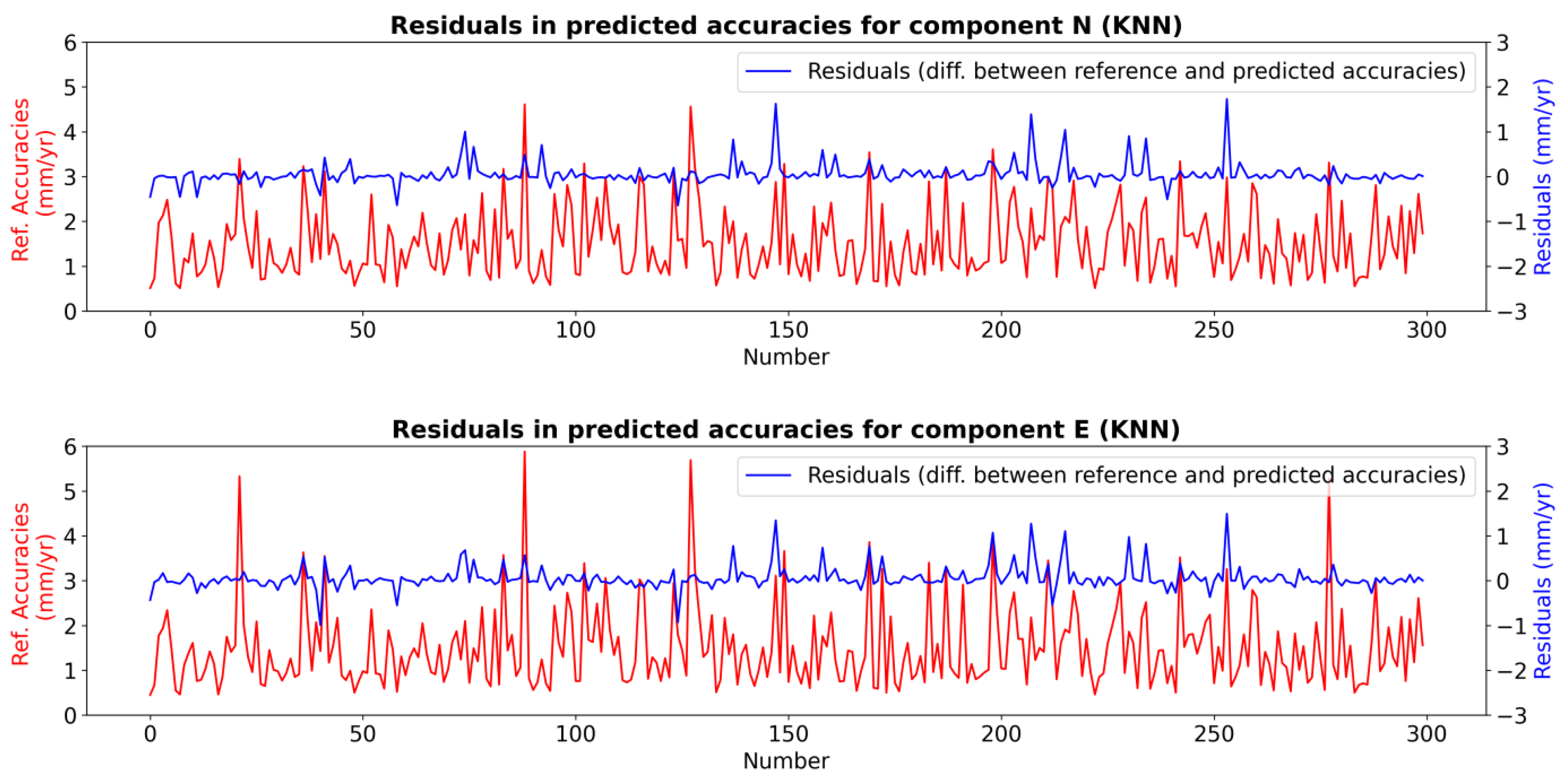
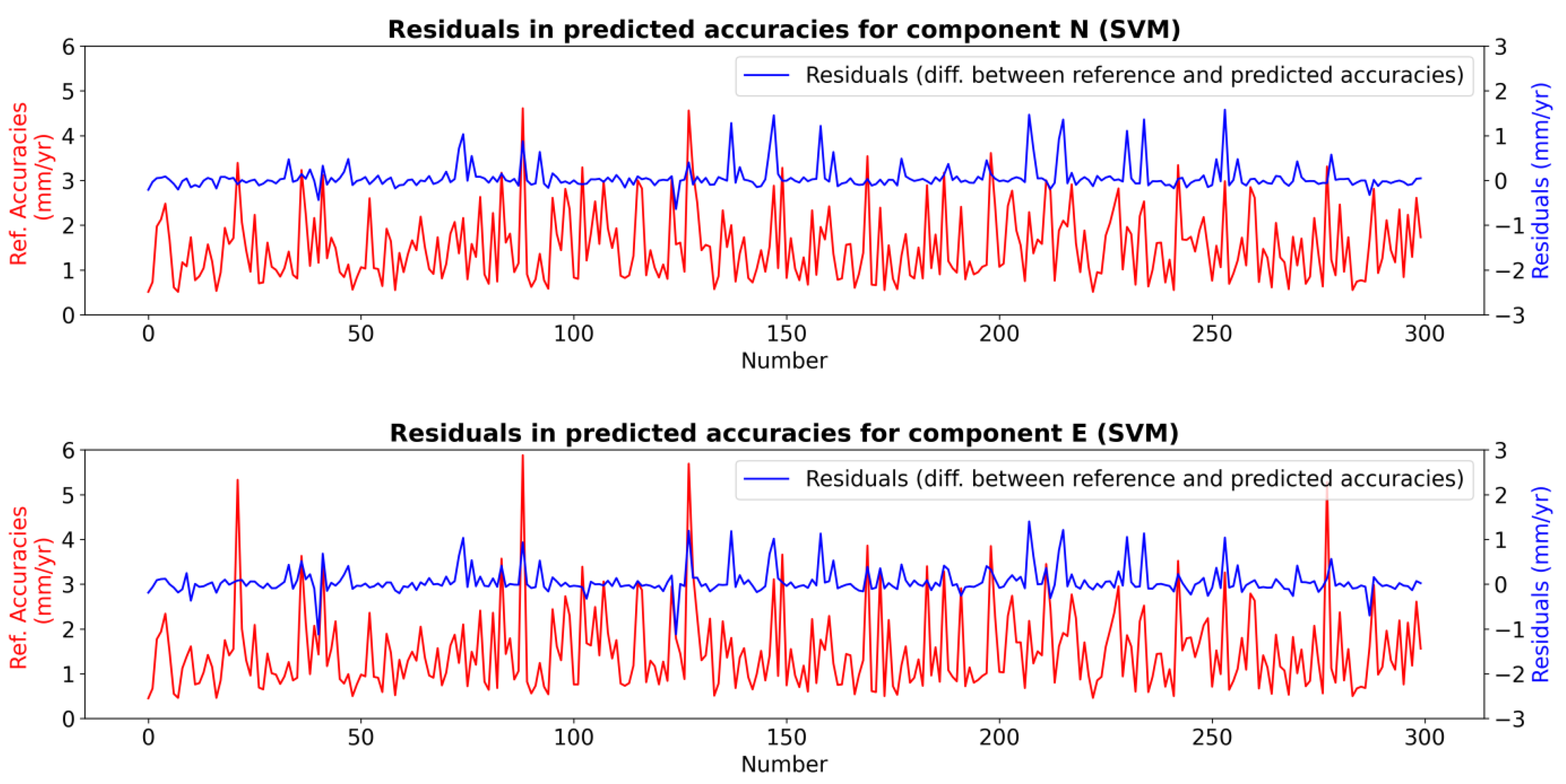
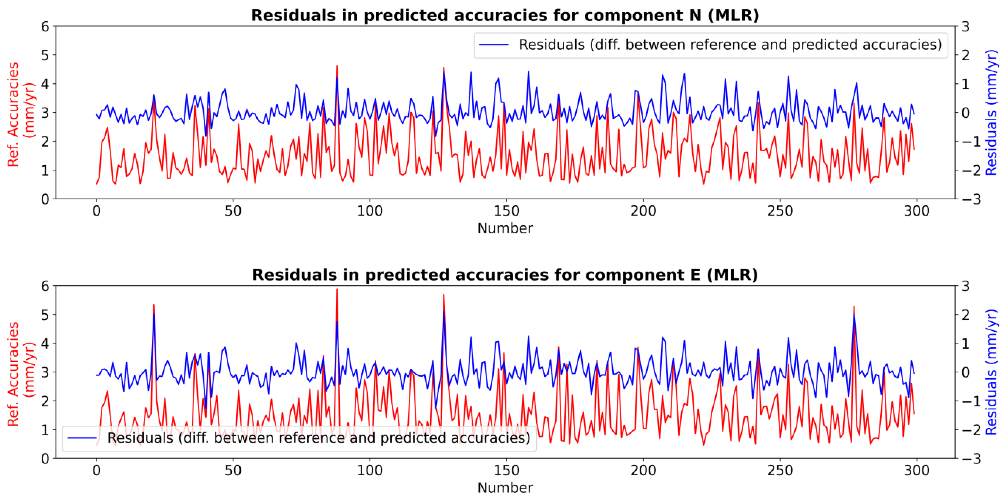
2.3. Training, Testing, and Results of the ML Model
3. Conclusions
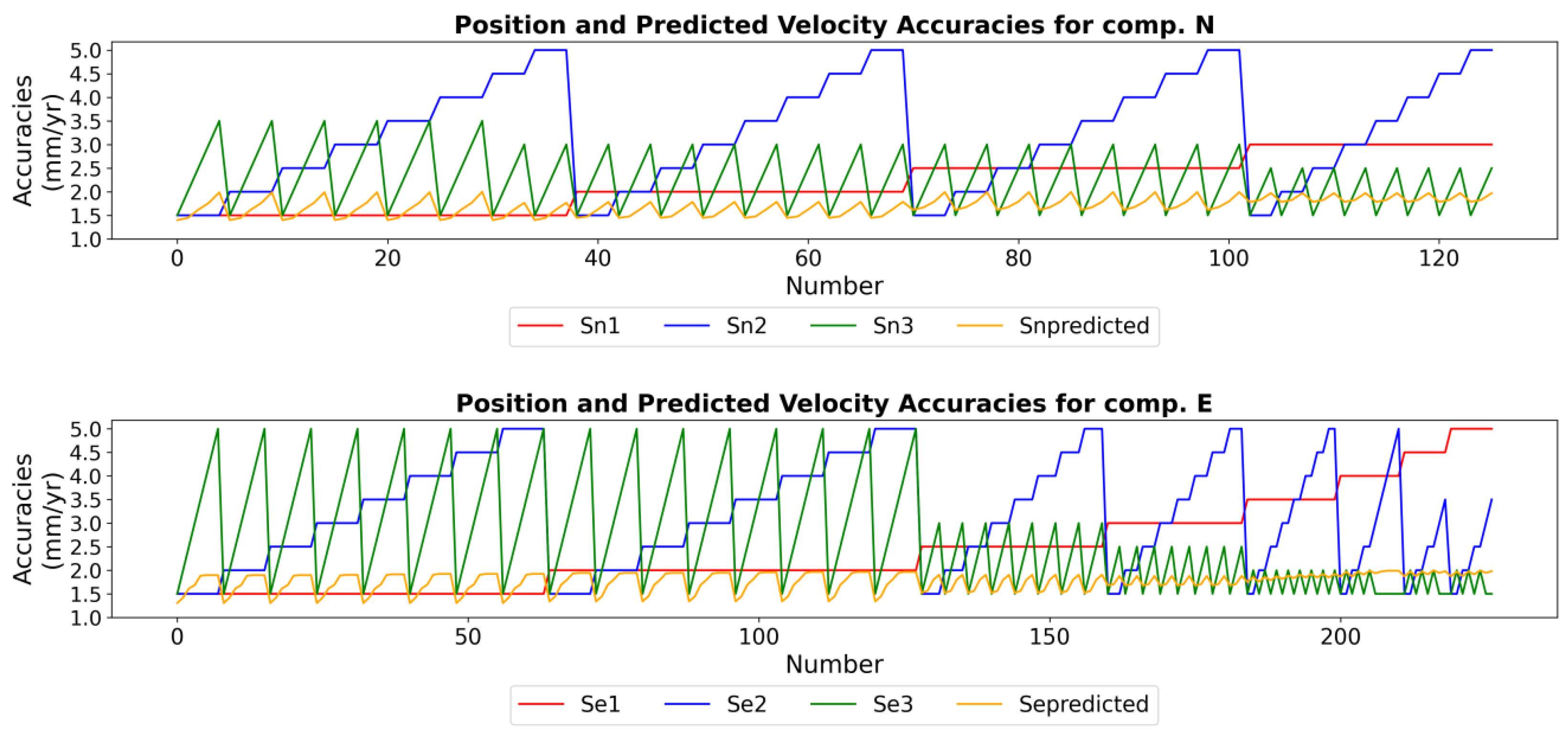
- East (E) Component: For 1-year interval GNSS data, achieving ±1.5 mm position accuracy per epoch resulted in a velocity accuracy greater than ±1 mm/year, with the best observed accuracy being ±1.3 mm/year. However, for 2- and 3-year interval datasets, submillimeter velocity accuracies could be achieved. Specifically, the best velocity accuracies were ±0.6 mm/year for 3-year intervals and ±0.7 mm/year for 2-year intervals.
- North (N) Component: Similarly, for 1-year interval GNSS data with ±1.5 mm position accuracy per epoch, the maximum attainable velocity accuracy was ±1.4 mm/year. For 2- and 3-year interval data, the best achievable velocity accuracies improved to ±0.6 mm/year for 3-year intervals and ±0.8 mm/year for 2-year intervals.
- Overall Observations: For GNSS campaigns conducted at 2- or 3-year intervals, velocity accuracies within ±1.5 mm/year are achievable for both components, provided the position accuracies remain below ±5 mm per epoch.
- The position accuracies of campaigns 1 and 3 had a more pronounced impact on velocity accuracy. However, as the positional accuracy of campaign 1 deteriorated, the influence of campaign 2’s positional accuracy became increasingly significant.
Funding
Institutional Review Board Statement
Informed Consent Statement
Data Availability Statement
Conflicts of Interest
References
- Uzel, T.; Eren, K.; Gulal, E.; Tiryakioglu, I.; Dindar, A.A.; Yilmaz, H. Monitoring the tectonic plate movements in Turkey based on the national continuous GNSS network. Arab. J. Geosci. 2013, 6, 3573–3580. [Google Scholar] [CrossRef]
- Özkan, A.; Solak, H.I.; Tiryakioğlu, İ.; Şentürk, M.D.; Aktuğ, B.; Gezgin, C.; Poyraz, F.; Duman, H.; Masson, F.; Uslular, G.; et al. Characterization of the co-seismic pattern and slip distribution of the February 06, 2023, Kahramanmaraş (Turkey) earthquakes (Mw 7.7 and Mw 7.6) with a dense GNSS network. Tectonophysics 2023, 866, 230041. [Google Scholar] [CrossRef]
- McClusky, S.; Balassanian, S.; Barka, A.; Demir, C.; Ergintav, S.; Georgiev, I.; Gurkan, O.; Hamburger, M.; Hurst, K.J.; Kahle, H.J.; et al. GPS constraints on crustal movements and deformations in the Eastern Mediterranean (1988–1997): Implications for plate dynamics. J. Geophys. Res. 2000, 105, 5695–5719. [Google Scholar] [CrossRef]
- Reilinger, R.; McClusky, S.; Vernant, P.; Lawrence, S.; Ergintav, S.; Cakmak, R.; Ozener, H.; Kadirov, F.; Guliev, I.; Stepanyan, R.; et al. GPS constraints on continental deformation in the Africa-Arabia-Eurasia continental collision zone and implications for the dynamics of plate interactions. J. Geophys. Res. Solid Earth 2006, 111, B05411. [Google Scholar] [CrossRef]
- Aktug, B.; Nocquet, J.M.; Cingöz, A.; Parsons, B.; Erkan, Y.; England, P.; Lenk, O.; Gürdal, M.A.; Kilicoglu, A.; Akdeniz, H.; et al. Deformation of western Turkey from a combination of permanent and campaign GPS data: Limits to block-like behavior. J. Geophys. Res. Solid Earth 2009, 114. [Google Scholar] [CrossRef]
- Yavaşoğlu, H.; Tarı, E.; Tüysüz, O.; Çakır, Z.; Ergintav, S. Determining and modeling tectonic movements along the central part of the North Anatolian Fault (Turkey) using geodetic measurements. J. Geodyn. 2011, 51, 339–343. [Google Scholar] [CrossRef]
- Ozener, H.; Dogru, A.; Acar, M. Determination of the displacements along the Tuzla fault (Aegean region-Turkey): Preliminary results from GPS and precise leveling techniques. J. Geodyn. 2013, 67, 13–20. [Google Scholar] [CrossRef]
- AKTUĞ, B.; Tiryakioğlu, I.; Sözbilir, H.; Özener, H.; Özkaymak, C.; Yiğit, C.O.; Solak, H.I.; Eyübagil, E.E.; Gelin, B.; Tatar, O.; et al. GPS derived finite source mechanism of the 30 October 2020 Samos earthquake, Mw = 6.9, in the Aegean extensional region. Turk. J. Earth Sci. 2021, 30, 718–737. [Google Scholar] [CrossRef]
- Eyübagil, E.E.; Solak, H.İ.; Kavak, U.S.; Tiryakioğlu, İ.; Sözbilir, H.; Aktuğ, B.; Özkaymak, Ç. Present-day strike-slip deformation within the southern part of İzmir Balıkesir Transfer Zone based on GNSS data and implications for seismic hazard assessment, western Anatolia. Turk. J. Earth Sci. 2021, 30, 143–160. [Google Scholar] [CrossRef]
- Solak, H.İ.; Tiryakioğlu, İ.; Özkaymak, Ç.; Sözbilir, H.; Aktuğ, B.; Yavaşoğlu, H.H.; Özkan, A. Recent tectonic features of Western Anatolia based on half-space modeling of GNSS Data. Tectonophysics 2024, 872, 230194. [Google Scholar] [CrossRef]
- Yilmaz, M.; Gullu, M. A comparative study for the estimation of geodetic point velocity by artificial neural networks. J. Earth Syst. Sci. 2014, 123, 791–808. [Google Scholar] [CrossRef]
- Langbein, J. Methods for rapidly estimating velocity precision from GNSS time series in the presence of temporal correlation: A new method and comparison of existing methods. J. Geophys. Res. Solid Earth 2020, 125, e2019JB019132. [Google Scholar] [CrossRef]
- Şafak, Ş.; Tiryakioğlu, İ.; Erdoğan, H.; Solak, H.İ.; Aktuğ, B. Determination of parameters affecting the accuracy of GNSS station velocities. Measurement 2020, 164, 108003. [Google Scholar] [CrossRef]
- Nocquet, J.M.; Calais, E. Crustal velocity field of western Europe from permanent GPS array solutions, 1996–2001. Geophys. J. Int. 2023, 154, 72–88. [Google Scholar] [CrossRef]
- Perez JA, S.; Monico JF, G.; Chaves, J.C. Velocity field estimation using GPS precise point positioning: The south American plate case. J. Glob. Position. Syst. 2023, 2, 90–99. [Google Scholar] [CrossRef]
- D’Anastasio, E.; De Martini, P.M.; Selvaggi, G.; Pantosti, D.; Marchioni, A.; Maseroli, R. Short-term vertical velocity field in the Apennines (Italy) revealed by geodetic levelling data. Tectonophysics 2006, 418, 219–234. [Google Scholar] [CrossRef]
- Özarpacı, S.; Kılıç, B.; Bayrak, O.C.; Taşkıran, M.; Doğan, U.; Floyd, M. Machine learning approach for GNSS geodetic velocity estimation. GPS Solut. 2024, 28, 65. [Google Scholar] [CrossRef]
- Kurt, A.İ.; Özbakir, A.D.; Cingöz, A.; Ergintav, S.; Doğan, U.; Özarpaci, S. Contemporary velocity field for Turkey inferred from combination of a dense network of long term GNSS observations. Turk. J. Earth Sci. 2023, 32, 275–293. [Google Scholar] [CrossRef]
- Reilinger, R.; McClusky, S. Nubia–Arabia–Eurasia plate motions and the dynamics of Mediterranean and Middle East tectonics. Geophys. J. Int. 2011, 186, 971–979. [Google Scholar] [CrossRef]
- Tiryakioğlu, İ.; Floyd, M.; Erdoğan, S.; Gülal, E.; Ergintav, S.; McClusky, S.; Reilinger, R. GPS constraints on active deformation in the Isparta Angle region of SW Turkey. Geophys. J. Int. 2013, 195, 1455–1463. [Google Scholar] [CrossRef]
- Konakoglu, B. Prediction of geodetic point velocity using MLPNN, GRNN, and RBFNN models: A comparative study. Acta Geod. Geophys. 2021, 56, 271–291. [Google Scholar] [CrossRef]
- Sorkhabi, O.M.; Alizadeh SM, S.; Shahdost, F.T.; Heravi, H.M. Deep learning of GPS geodetic velocity. J. Asian Earth Sci. X 2022, 7, 100095. [Google Scholar]
- Mitchell, T.M. Does machine learning really work? AI Mag. 1997, 18, 11. [Google Scholar]
- Flach, P. Machine Learning: The Art and Science of Algorithms That Make Sense of Data; Cambridge University Press: Cambridge, UK, 2012. [Google Scholar]
- Griffiths, J. Combined orbits and clocks from IGS second reprocessing. J. Geod. 2019, 93, 177–195. [Google Scholar] [CrossRef] [PubMed]
- Petit, G.; Luzum, B. The 2010 reference edition of the IERS conventions. In Reference Frames for Applications in Geosciences; Springer: Berlin/Heidelberg, Germany, 2013; pp. 57–61. [Google Scholar]
- Huang, J.; He, X.; Hu, S.; Ming, F. Impact of Offsets on GNSS Time Series Stochastic Noise Properties and Velocity Estimation. Adv. Space Res. 2024; in press. [Google Scholar] [CrossRef]
- Herring, T.A.; King, R.W.; Floyd, M.A.; McClusky, S.C. Introduction to GAMIT/GLOBK; Release 10.7; Massachusetts Institute of Technology: Cambridge, MA, USA, 2018; 54p, Available online: http://geoweb.mit.edu/gg/docs/Intro_GG.pdf (accessed on 20 November 2024).
- Crocetti, L.; Schartner, M.; Soja, B. Discontinuity detection in GNSS station coordinate time series using machine learning. Remote Sens. 2021, 13, 3906. [Google Scholar] [CrossRef]
- Sykes, A.O. An Introduction to Regression Analysis; Chicago Working Paper in Law & Economics; University of Chicago Law School: Chicago, IL, USA, 1993; p. 20. [Google Scholar]
- Araghinejad, S. Data-Driven Modeling: Using MATLAB® in Water Resources and Environmental Engineering; Water Science and Technology Library; Springer: Dordrecht, The Netherlands, 2014; Volume 67. [Google Scholar]
- Kaya, H.; Gündüz-Öğüdücü, Ş. A distance based time series classification framework. Inf. Syst. 2015, 51, 27–42. [Google Scholar] [CrossRef]
- Wang, L. Support Vector Machines: Theory and Applications; Springer Science & Business Media: Berlin/Heidelberg, Germany, 2005; Volume 177. [Google Scholar]
- Breiman, L. Random forests. Mach. Learn. 2001, 45, 5–32. [Google Scholar] [CrossRef]
- Guo, L.; Chehata, N.; Mallet, C.; Boukir, S. Relevance of airborne lidar and multispectral image data for urban scene classification using random forests. ISPRS J. Photogramm. Remote Sens. 2011, 66, 56–66. [Google Scholar] [CrossRef]
- Rodriguez-Galiano, V.F.; Ghimire, B.; Rogan, J.; Chica-Olmo, M.; Rigol-Sánchez, J.P. An assessment of the effectiveness of a random forest classifier for land-cover classification. ISPRS J. Photogramm. Remote Sens. 2012, 67, 93–104. [Google Scholar] [CrossRef]
- Belgiu, M.; Drăguţ, L. Random Forest in remote sensing: A review of applications and future directions. ISPRS J. Photogramm. Remote Sens. 2016, 114, 24–31. [Google Scholar] [CrossRef]
- Rodriguez-Galiano, V.; Sanchez-Castillo, M.; Chica-Olmo, M.; Chica-Rivas, M. Machine learning predictive models for mineral prospectivity: An evaluation of neural networks, random forest, regression trees and support vector machines. Ore Geol. Rev. 2015, 71, 804–818. [Google Scholar] [CrossRef]
- Modaresi, F.; Araghinejad, S.; Ebrahimi, K. A Comparative Assessment of Artificial Neural Network, Generalized Regression Neural Network, Least-Square Support Vector Regression, and K-Nearest Neighbor Regression for Monthly Streamflow Forecasting in Linear and Nonlinear Conditions. Water Resour Manag. 2018, 32, 243–258. [Google Scholar] [CrossRef]
- Kazemi, F.; Asgarkhani, N.; Jankowski, R. Optimization-based stacked machine-learning method for seismic probability and risk assessment of reinforced concrete shear walls. Expert Syst. Appl. 2024, 255, 124897. [Google Scholar] [CrossRef]
- Kazemi, F.; Asgarkhani, N.; Jankowski, R. Machine learning-based seismic fragility and seismic vulnerability assessment of reinforced concrete structures. Soil Dyn. Earthq. Eng. 2023, 166, 107761. [Google Scholar] [CrossRef]
- Eckl, M.C.; Snay, R.A.; Soler, T.; Cline, M.W.; Mader, G.L. Accuracy of GPS-derived relative positions as a function of interstation distance and observing-session duration. J. Geod. 2001, 75, 633–640. [Google Scholar] [CrossRef]


| Variable Name | Variable Type | Dataset No | Value Type | Details |
|---|---|---|---|---|
| Year Interval | Input | 1 and 2 | Integer | Number of years between measurements |
| Se1 | Input | 1 | Decimal | Position accuracy for the E component of the first measurement, independent of the measurement time |
| Se2 | Input | 1 | Position accuracy for the E component of the second measurement, independent of the measurement time | |
| Se3 | Input | 1 | Position accuracy for the E component of the third measurement, independent of the measurement time | |
| Sve | Output | 1 | Velocity accuracy for the E component | |
| Sn1 | Input | 2 | Position accuracy for the N component of the first measurement, independent of the measurement time | |
| Sn2 | Input | 2 | Position accuracy for the N component of the second measurement, independent of the measurement time | |
| Sn3 | Input | 2 | Position accuracy for the N component of the third measurement, independent of the measurement time | |
| Svn | Output | 2 | Velocity accuracy for the N component |
| Variable | Count | Mean | std | min. | 25% | 50% | 75% | max. |
|---|---|---|---|---|---|---|---|---|
| year interval | 1500 | 2 | 0.816769 | 1 | 1 | 2 | 3 | 3 |
| Se1 | 1500 | 3.8 | 2.347546 | 1.63 | 2.19 | 2.79 | 4.07 | 8.37 |
| Sn1 | 1500 | 3.45438 | 1.476844 | 1.73 | 2.43 | 3.07 | 4.06 | 6.49 |
| Se2 | 1500 | 4.257367 | 2.965279 | 1.59 | 2.36 | 2.85 | 3.86 | 11.2 |
| Sn2 | 1500 | 3.8696 | 1.86619 | 1.7 | 2.51 | 3.21 | 4.45 | 8.55 |
| Se3 | 1500 | 3.411333 | 1.982387 | 1.59 | 2.0875 | 2.5 | 3.5225 | 7.93 |
| Sn3 | 1500 | 3.279 | 1.329525 | 1.7 | 2.2875 | 2.765 | 3.7525 | 6.78 |
| SVe | 1500 | 1.52856 | 0.985174 | 0.45 | 0.8475 | 1.27 | 1.91 | 6.83 |
| SVn | 1500 | 1.514887 | 0.79991 | 0.51 | 0.9 | 1.3 | 1.96 | 4.83 |
| ML Algorithms | Train and Test Results | |||||||
|---|---|---|---|---|---|---|---|---|
| MLR | SVM | RF | KNN | |||||
| Components | E | N | E | N | E | N | E | N |
| Train Score (%) | 72 | 76 | 92 | 91 | 97 | 98 | 94 | 94 |
| Test Score (%) | 71 | 72 | 90 | 86 | 95 | 97 | 91 | 89 |
| Avg. Train RMSE (mm/year) | 0.5 | 0.4 | 0.3 | 0.2 | 0.2 | 0.1 | 0.2 | 0.2 |
| Avg. Test RMSE (mm/year) | 0.5 | 0.4 | 0.3 | 0.3 | 0.2 | 0.1 | 0.3 | 0.3 |
| Position Accuracies (mm) | Velocity Accuracy (mm/yr) | Predicted Velocity Accuracy (mm/yr) | |||||||
|---|---|---|---|---|---|---|---|---|---|
| Station Number | Se1 | Se2 | Se3 | Sv | MLR | SVM | RF | KNN | |
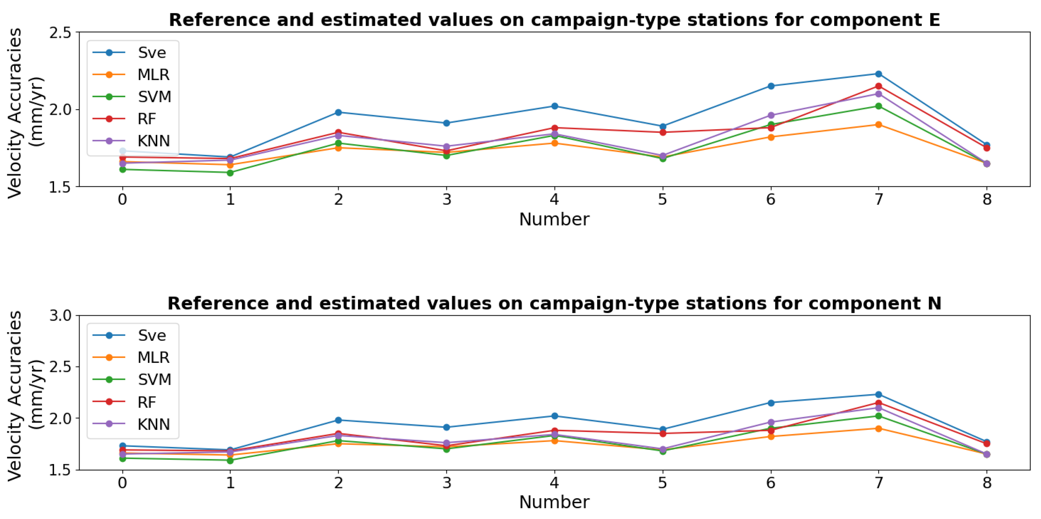
| East Component | 1 | 2.97 | 1.82 | 1.82 | 1.73 | 1.66 | 1.61 | 1.69 | 1.65 |
| 2 | 3.14 | 1.36 | 1.71 | 1.69 | 1.64 | 1.59 | 1.68 | 1.67 | |
| 3 | 2.97 | 1.82 | 2.43 | 1.98 | 1.75 | 1.78 | 1.85 | 1.83 | |
| 4 | 3.14 | 1.36 | 2.19 | 1.91 | 1.72 | 1.70 | 1.73 | 1.76 | |
| 5 | 2.97 | 2.05 | 2.53 | 2.02 | 1.78 | 1.83 | 1.88 | 1.84 | |
| 6 | 2.81 | 1.53 | 2.34 | 1.89 | 1.69 | 1.68 | 1.85 | 1.70 | |
| 7 | 3.1 | 1.65 | 2.75 | 2.15 | 1.82 | 1.90 | 1.88 | 1.96 | |
| 8 | 3.48 | 2.08 | 2.64 | 2.23 | 1.90 | 2.02 | 2.15 | 2.10 | |
| 9 | 2.3 | 2.05 | 2.53 | 1.77 | 1.65 | 1.65 | 1.75 | 1.65 | |
| North Component | 1 | 3.72 | 2.18 | 2.05 | 2.06 | 1.97 | 1.97 | 2.08 | 2.10 |
| 2 | 3.98 | 1.65 | 1.91 | 2.01 | 1.97 | 1.93 | 2.07 | 2.11 | |
| 3 | 3.72 | 2.18 | 3.02 | 2.45 | 2.12 | 2.32 | 2.42 | 2.29 | |
| 4 | 3.98 | 1.65 | 2.65 | 2.36 | 2.09 | 2.17 | 2.31 | 2.22 | |
| 5 | 3.25 | 2.43 | 2.79 | 2.22 | 2.00 | 2.10 | 2.11 | 2.08 | |
| 6 | 3.57 | 1.76 | 2.88 | 2.35 | 2.04 | 2.16 | 2.37 | 2.18 | |
| 7 | 4.05 | 1.98 | 3.06 | 2.58 | 2.19 | 2.41 | 2.51 | 2.36 | |
| 8 | 4.36 | 2.43 | 3.2 | 2.74 | 2.30 | 2.64 | 2.54 | 2.46 | |
| 9 | 2.51 | 2.43 | 2.79 | 1.93 | 1.84 | 1.84 | 1.94 | 1.90 | |
Disclaimer/Publisher’s Note: The statements, opinions and data contained in all publications are solely those of the individual author(s) and contributor(s) and not of MDPI and/or the editor(s). MDPI and/or the editor(s) disclaim responsibility for any injury to people or property resulting from any ideas, methods, instructions or products referred to in the content. |
© 2024 by the author. Licensee MDPI, Basel, Switzerland. This article is an open access article distributed under the terms and conditions of the Creative Commons Attribution (CC BY) license (https://creativecommons.org/licenses/by/4.0/).
Share and Cite
Solak, H.İ. Prediction of GNSS Velocity Accuracies Using Machine Learning Algorithms for Active Fault Slip Rate Determination and Earthquake Hazard Assessment. Appl. Sci. 2025, 15, 113. https://doi.org/10.3390/app15010113
Solak Hİ. Prediction of GNSS Velocity Accuracies Using Machine Learning Algorithms for Active Fault Slip Rate Determination and Earthquake Hazard Assessment. Applied Sciences. 2025; 15(1):113. https://doi.org/10.3390/app15010113
Chicago/Turabian StyleSolak, Halil İbrahim. 2025. "Prediction of GNSS Velocity Accuracies Using Machine Learning Algorithms for Active Fault Slip Rate Determination and Earthquake Hazard Assessment" Applied Sciences 15, no. 1: 113. https://doi.org/10.3390/app15010113
APA StyleSolak, H. İ. (2025). Prediction of GNSS Velocity Accuracies Using Machine Learning Algorithms for Active Fault Slip Rate Determination and Earthquake Hazard Assessment. Applied Sciences, 15(1), 113. https://doi.org/10.3390/app15010113