Abstract
Urban rail transit passenger flow forecasting often relies on the traditional “four-step” method, where the division of traffic analysis zones (TAZs) is critical to ensuring prediction accuracy. As the fundamental units for describing trip origins and destinations, TAZs also encompass socioeconomic attributes such as land use, population, and employment. However, traditional TAZs, typically based on administrative boundaries, fail to reflect evolving urban travel behavior, particularly when transit stations are located near TAZ boundaries. Additionally, the emergence of urban big data allows for more refined spatial analyses based on individual travel patterns, addressing the limitations of administrative divisions. This study proposes an innovative TAZ aggregation model based on travel similarity, integrating public transit smart-card data and GIS data from bus networks. First, individual spatiotemporal travel patterns are mapped and discretized in both the spatial and temporal dimensions. Travel characteristic data are then extracted for spatial grid units. The TAZ division problem is defined as a multiobjective optimization problem, including factors such as travel similarity, the homogeneity of travel intensity, the statistical accuracy of the area, geographic information preservation, travel ratio constraints, and shape constraints. Multiple TAZ division schemes are produced and assessed using the Technique for Order Preference by Similarity to Ideal Solution (TOPSIS), resulting in the selection of the optimal scheme. The proposed method is implemented on bus passenger travel data in Beijing, showing that the optimized scheme significantly reduces the number of zones with travel ratios exceeding 10%. Compared with existing schemes, the optimized division yields more uniform distributions of travel ratios, area, and travel density, while significantly minimizing the number of zones with a high travel concentration. These results demonstrate that the proposed method better reflects residents’ actual travel behaviors, offering a notable improvement over traditional approaches. This research provides a novel and practical framework for data-driven TAZ optimization.
1. Introduction
In current urban rail transit planning, the basic unit for passenger flow demand analysis and prediction is the traffic analysis zone (TAZ) (also referred to as a traffic zone) [1]. TAZs are based on or conform to administrative divisions, and for areas that have been investigated using an origin–destination (OD) matrix, the original division of the zones is preserved as much as possible. The applicability of the TAZ scheme significantly affects the results of passenger demand analysis and forecasting [2,3], as well as traffic safety [4,5] and the scientific reliability and rationality of transportation planning [6,7]. An effective TAZ division scheme aids in the development of macroscopic traffic prediction models [1,7,8,9,10,11]. However, a unified standard and relevant regulations for TAZ division are absent both domestically and internationally. In urban planning practice, practical experience and the principle of traffic district division serve as the primary basis for the division of traffic districts [12]. Where possible, engineering practice has outlined a series of traffic district division principles, such as subdistricts based on land use and economic and social characteristics, to maintain consistency and satisfy the principle of homogeneity, and to avoid breaking the division of administrative subdivisions, thus enabling the use of existing statistical data on the administrative district [13]. However, these division principles are all qualitative guidelines and lack a solid quantitative foundation; thus, traffic district division plans based on these qualitative principles are often highly subjective. Moreover, when dividing TAZs, if the zones are too large, some geographical information and regional travel proportions may be lost, and if they are too small, it may decrease statistical accuracy. Additionally, when the spatial partitioning system used for collecting and analyzing data is variable or arbitrary, the modifiable areal unit problem (MAUP) can occur, which involves two main issues: the scale effect and the zoning effect. The scale effect denotes a phenomenon where the analysis results change as spatial data are aggregated, changing their granularity or cell size. The zoning effect denotes a phenomenon where the analysis results change based on different aggregation methods (i.e., zoning schemes) at the same level of granularity and aggregation.
Some studies have tried using relevant surveys and data-driven approaches to extract additional feature information in order to classify traffic neighborhoods. For example, based on traditional traffic neighborhoods that only convey geographical attributes, Jing Lian and colleagues applied deep neural networks to extract high-dimensional data such as spatial geographic attributes and vehicle trip information. They identified the most relevant features of trip origins and destinations through statistical measurements of relevance, constructing trip-based traffic neighborhoods while integrating various kinds of auxiliary information [14]. Marisdea and colleagues, building on traditional traffic neighborhood delineation, derived potential land use and spatiotemporal mobility features based on big data and enhanced the traditional model using a multivariate data-driven approach. They integrated vehicle data with traffic neighborhoods to define regional configurations of origins and destinations for demand forecasting, aiming to minimize trips within the region [15]. Zhang Xinyue and colleagues introduced data such as license plate information, transforming an intersection node OD matrix into rules for a traffic neighborhood OD matrix. They demonstrated the effectiveness of the traffic neighborhood transformation rules through two indicators: traffic allocation and the detection of traffic deviation [16]. Gao Yue’er and colleagues introduced a spatial analysis method that combines dynamic traffic state characteristics with static road network features to define tourist traffic neighborhoods [17]. Furthermore, Wang Xiaoquan and colleagues, when studying vehicle ownership behavior, examined the spatial correlation between traffic neighborhoods. Based on travel survey data from Changchun residents, they calculated the model parameters, confirming that the spatial correlation characteristics of traffic neighborhoods, such as residential density, land use mix, intersection density, and public transportation stop density, all significantly negatively affect household vehicle ownership [18]. The aforementioned studies introduce additional survey data based on traditional traffic neighborhood division. Although these studies have achieved good results for specific areas, on the one hand, additional survey data are not easily obtained on a large scale, and on the other hand, the increased data requirements of these methods reduce their versatility, making them difficult to apply to traffic neighborhood division research and other regions. With regard to the forms of traffic neighborhood division, Wu Dawei and colleagues explored the application of fine-grid management methods in transportation planning. Based on a case study in Chuanhui, China, they proposed a data-driven fine-grid division method for determining TAZs. The results showed that the fine-grid division method for determining TAZs based on quadrilateral grids can achieve lower levels of predictive value bias and variable correlation bias when the number of TAZs is large [19]. In addition, Mehdi and colleagues examined the impacts of different regular geometric shapes on traffic demand issues. They divided TAZs into squares, rhombuses, triangles, and hexagons, then conducted a detailed evaluation of the changes in various metrics between the traditional TAZ division method and the division method with different geometries. The results confirmed the effectiveness of the regular division method [1]. Marta and colleagues used the smallest available census units to divide traffic neighborhoods and employed a geographically weighted negative binomial regression model for a comparative analysis of macro-crash prediction. The results indicated that some features of the built environment are significant predictors of traffic crashes, and the new division method can better capture the differences between these features and traffic safety in different spaces [20]. In addition to considering the static spatial constraints of traffic neighborhoods, some studies have considered the dynamic development of traffic neighborhoods. Considering that regional development may lead to the reclassification of existing transportation subdivisions, Yao Hong and colleagues introduced six methods of assigning travel data to rezoned transportation subdivisions. Illustrated using 2001 and 2016 travel data from Toronto, Canada, the results confirmed the significant impact of different traffic neighborhood division methods on transportation policy [21]. The aforementioned methods, regarding the form of the dynamic and static subdivision of traffic neighborhoods, have partly confirmed the impact of traffic neighborhood shape on the mapping of spatial relationships. However, no further research has been conducted on the division principles, limiting the improvement of the division results of these studies. Regarding the division principles, a series of works have also been developed to improve the clustering methods used in traditional traffic neighborhood division. For example, to provide features more in line with passengers’ travel needs, Song Li Jing and colleagues proposed traffic neighborhoods based on the division of bus passenger corridors. They divided the corridor into two levels: the direct impact area and indirect impact area. Through big data, they selected more suitable clustering indices for traffic neighborhood division and introduced clustering factors to improve the accuracy deficit of traditional clustering methods [22]. Wang Jun and colleagues took the locations of smart-card ports on urban roads as the clustering object and implemented a new DBSCAN clustering algorithm. They used contour coefficients to evaluate the quality of clustering, enabling the rapid division of urban traffic neighborhoods [23]. With the rapid development of urban transportation systems, the travel structure of urban residents has undergone significant changes. For example, according to the results of the Fifth Resident Travel Survey in Beijing, the proportion of public transportation trips increased from 30% in 2005 to 50% in 2014, with the proportion of rail transit trips continuously increasing [24]. However, suppose that rail transit stations are located at the boundaries of traffic neighborhoods. In that case, actual travel will significantly differ from travel centered on the traffic neighborhood, leading to decreased prediction accuracy [25]. Furthermore, when the spatial partitioning system used for collecting and analyzing data is variable or arbitrary, the modifiable areal unit problem (MAUP) may arise [5,26]. In response to the MAUP issue in the process of traffic neighborhood division, Amoh and colleagues [27] studied several spatial cells that can be used as TAZs, including statistical area levels, postal districts, state election districts, grid cells, and the Tyson polygon Melbourne integrated traffic model developed around the center of mass. The aforementioned clustering-based methods often use fuzzy clustering, k-means, and other clustering algorithms, generally based on administrative divisions or city university data for traffic neighborhood division. The former improves upon the administrative division method, emphasizing the feasibility of the method, which is not suitable for engineering practice; the latter builds models based on spatial and agglomeration features formed by urban big data, with relatively single indicators, that cannot fully capture the rationality of traffic neighborhood division.
Most existing studies on traffic zone aggregation rely on clustering methodologies such as fuzzy clustering and k-means clustering algorithms. One category of methods uses travel information, socioeconomic attributes, and land-use characteristics within administrative divisions to construct features of travel similarity and spatial similarity for traffic zone division. Since these methods depend on traditional data and subdivide or merge traffic zones based on administrative boundaries, their primary goal is to demonstrate the feasibility of traffic zone division methods. However, such approaches are unsuitable for practical engineering applications. Another category of studies uses urban big data for traffic zone division. These methods build models using features such as spatial similarity, travel similarity, and aggregation derived from urban big data. However, the metrics used to describe traffic zones in such studies are relatively limited and are unable to fully capture the process of traffic zone division. Based on the aforementioned issues, in this study, we intend to use individual travel data and their spatiotemporal discrete mapping relationships, combined with the quantitative principles of traffic neighborhood division, to comprehensively investigate aspects such as travel similarity, homogeneity, statistical accuracy, and geographic information loss. We propose a spatial optimization model for traffic neighborhoods. A series of optimization schemes are divided automatically based on the objective function and constraints, and then, the optimal traffic neighborhood division scheme is selected according to the evaluation indices. The effectiveness of the method proposed in this paper is validated using bus travel data from downtown Beijing.
Taking China as an example, many cities in China have adopted bus smart cards, and the bus line coverage and bus travel proportion of large cities are relatively high. The obtained passenger flow results reflect urban bus operations and residents’ bus travel characteristics. Taking Beijing as an example, as of June 2017, Beijing has 1730 bus lines, a 500 m station coverage rate of 80%, and a line network coverage rate of 78%; in 2015, the bus coverage within the Fourth Ring Road had reached more than 97%, and the proportion of urban public electric vehicles that transported passengers was 48.2%. Therefore, the spatial and temporal activity distribution of residents in the central urban area can be effectively described based on bus card data.
2. Data Preprocessing
In this study, a model is built using individual travel data from public transportation in Beijing, taking bus smart-card data as an example, which contain temporal and spatial information on individual travel. Combined with spatial data, the individual travel data are discretized in both space and time to generate the required spatiotemporal data for the model.
2.1. Data Cleaning
In this paper, a model is built using individual travel data from public transport (specifically, bus smart-card data containing spatiotemporal information on individual travel). The spatiotemporal mapping and discretization of individual travel data are performed using spatial data to generate the spatiotemporal data required for the model.
Currently, the main public transportation billing methods are divided into two categories: the one-ticket system and segmented billing. The former only requires passengers to swipe their cards when boarding and alighting, while the latter charges passengers based on the distance traveled, which is determined based on the boarding and alighting points. The 2016 Beijing public transportation smart-card data used in this study contain the following data abnormalities: (1) passengers boarding and alighting at the same station, resulting in the same starting and ending points; (2) passengers’ alighting time being earlier than or equal to their boarding time, resulting in erroneous data; (3) passengers’ travel time being inconsistent with their travel distance, leading to speeds outside the normal range; (4) data being duplicated due to system errors; (5) data being incomplete due to passengers forgetting to swipe their cards or failing to swipe them successfully; (6) the duration of a single trip exceeding 4 h (in 2016, Beijing implemented a segmented charging rule, which prevents passengers from swiping their cards on the same route within 4 h; otherwise, it results in abnormal charges).
For the first five types of data quality issues, constraints and rules were applied directly in the database to filter and delete erroneous entries. For the sixth issue, following the method proposed by Yue Zhenhong [28], card swiping behavior was divided into “goodwill swipes” and “malicious swipes”. The corresponding technique was applied to correct anomalous data, and data that remained erroneous after correction were deleted. “Goodwill swipes” refers to when passengers swipe their cards in advance to avoid missing their stop, while “malicious swipes” refers to when passengers swipe their cards ahead of time to reduce the fare.
2.2. Space–Time Mapping and Discretization
As a common kind of individual travel data, bus smart-card data include the card number, station number, boarding/alightment time, bus line, station, etc. The geographic information of the bus network is used as spatial data, including the names and numbers of bus lines and stations, and line routing information. The two types of data are matched through the line of passengers getting on and off the bus and the station coding rules, and the travel data are matched with the space line network to obtain the travel information of passengers getting on and off the bus at the station (see Equation (1)). Here, represents the travel information of passenger i, including information on boarding time , boarding station , alighting time , and alighting station (see Equation (2)).
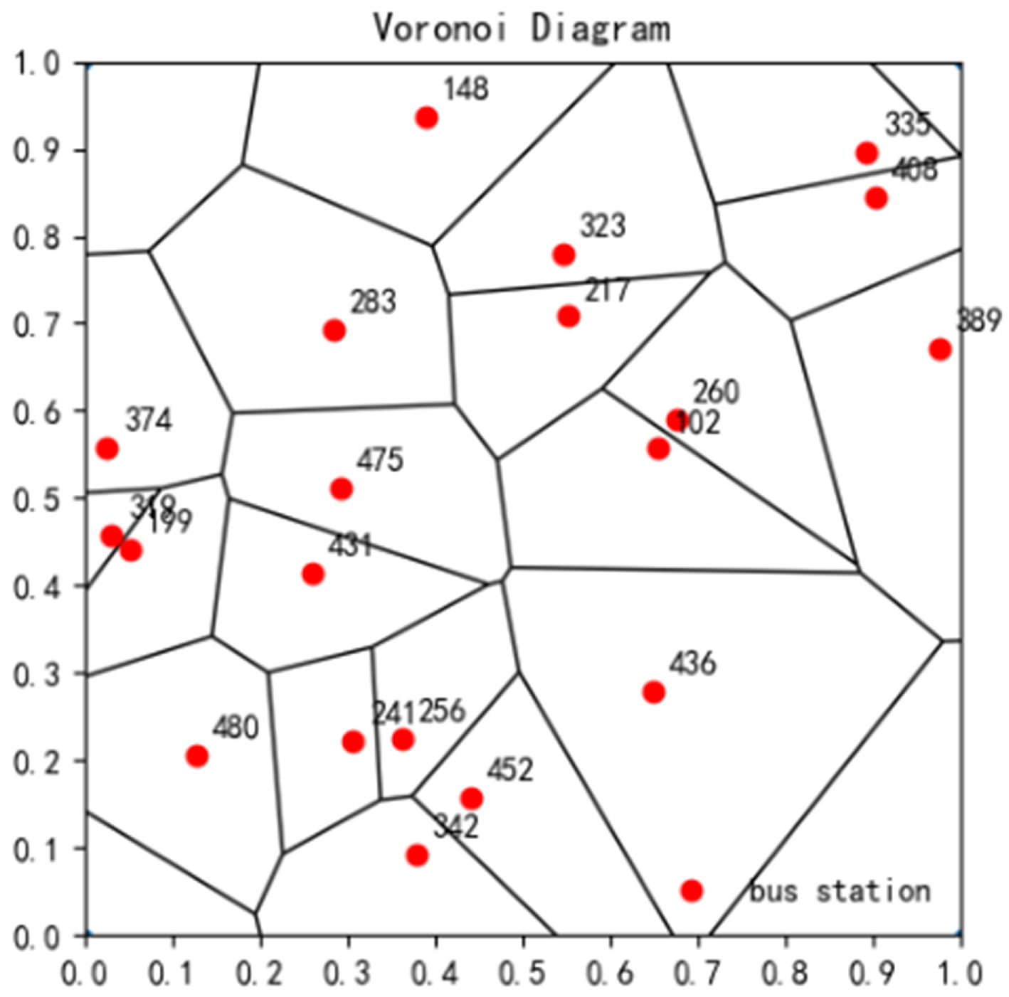
In the spatial dimension, according to the passenger travel information at station , the total number of trips at the corresponding station and the number of trips between different stations are obtained. Then, based on the distribution of bus stations, the Delaunay triangulation method is used to divide the space into Tyson polygon areas centered on a bus station. Then, the total number of trips of station is mapped to the corresponding Tyson polygon area , where a Delaunay triangular mesh is applied; this is a triangular meshing method based on the construction of a given set of points, and for any triangle, its outer circle contains no other points.Assuming that there are 20 randomly distributed bus stations, the Delaunay triangular mesh method is divided as shown in Figure 1, where the different bus stations and their corresponding trip volumes are indicated. The abscissa and ordinate in Figure 1 represent the normalized position of the bus station on the two-dimensional plane, reflecting the relative geometric relationship between the stations. The location of the station is represented by a normalized dimensionless unit, which is evenly distributed in the area.
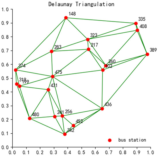
Figure 1.
Delineation diagram of Delaunay triangulation of bus stations.
The Tyson polygon is dual to the Delaunay triangulation, and by using the perpendicular bisector of the line joining the centers of the outer circles of the Delaunay triangle as a boundary, the Tyson polygon corresponding to that point is obtained. The Tyson polygon consists of all points that are closer to the seed point of that polygon than any other seed point, and can be mathematically represented as
In Equation (3), denotes the Tyson polygon with h as the seed point, and denotes the distance between x and y. The Tyson polygon obtained on the basis of Figure 1 is shown in Figure 2.
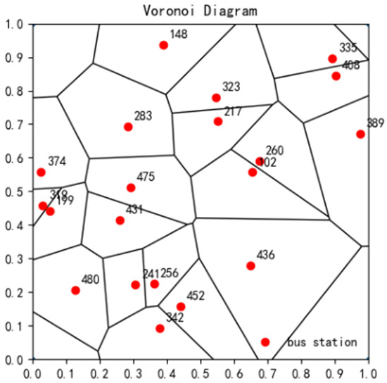
Figure 2.
Tyson polygon division diagram of bus stations.
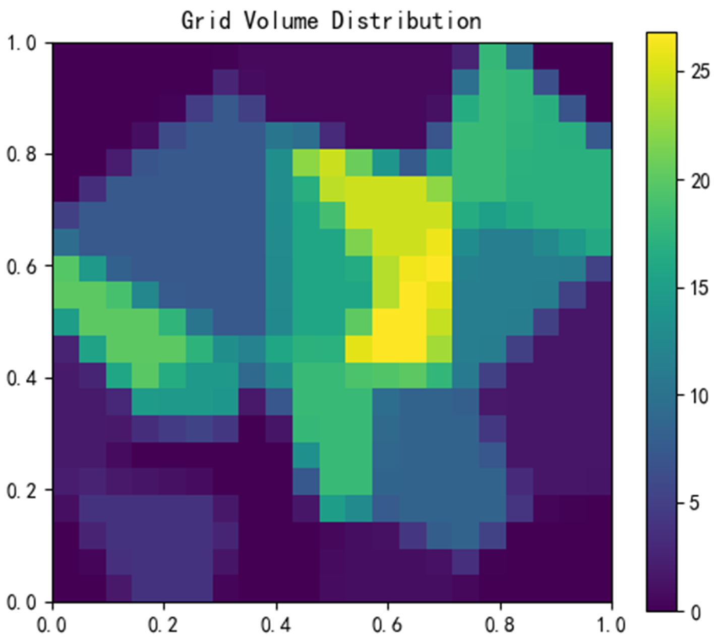
Finally, a square grid is used to spatially discretize the area to be studied, and a discretized spatial cell is obtained. According to the spatial mapping relationship between the discretized cell and the Tyson polygon, the trips in the Tyson polygonal area are discretized into the spatial cell using the area-weighting method, and the total number of trips corresponding to each grid is obtained, as shown in Figure 3, with the thermal value of the cell representing its trip volume. The purpose of the area-weighting method is to discretize the plane in Figure 2 into a uniform grid unit of , calculate the intersection area of each polygon and the grid unit, and allocate the total travel volume of the bus station to the intersecting grid unit according to the area ratio.

Figure 3.
Discrete cell schematic diagram of bus stations.
The travel volume in cell k can be calculated using Equation (4), where denotes the area occupied by the Tyson polygonal region in cell k, denotes the total number of trips corresponding to site , denotes the total area of the Tyson polygonal region , and m denotes the number of polygons intersecting with .
On the basis of spatial discretization, according to the fixed time interval, the total number of passengers boarding and alighting at each station in each time period of the day is counted, and the similarity of passenger flow time distribution between stations is calculated using the correlation coefficient. The calculation method is shown in Equations (5) and (6).
where is the total number of passengers getting on and off the bus at station i in time period t. There are 48 time periods t, of which the first 24 represent the passenger flow at the first bus station, and the last 24 represent the passenger flow at the second bus station; n is the number of bus stations; and are the average passenger flow of stations i and j, respectively; and and are the passenger flow variance of stations i and j, respectively. The calculation result is a matrix of , which represents the similarity of passenger flow time distribution between two bus stations.
2.3. Basic Data Construction
Based on the spatiotemporal discrete travel data, the spatial grid attribute data are constructed for the TAZ division model.
(1) Adjacency matrix M of cells: This describes the adjacency relationship between discrete-space cells, which is a sparse matrix, as shown in Equation (7). K is the total number of cells in the study area. When cells i and j share an edge, the two cells are considered to be adjacent, in which case, is 1; otherwise, is 0.
(2) Travel time similarity of cells : This is a numerical matrix, as shown in Equation (6). The travel time correlations between this cell and other cells are described by and the Pearson correlation coefficient , as shown in Equation (9). Here, and are the average trips of cells i and j, respectively; and are the variance of the trips of cells i and j.
(3) Cell area A: This describes the space area of each cell, where K is the number of cells, as shown in Equation (8). Since square isometric grids are adopted in this study, the area of all cells is equal.
(4) The distance between cell centroids D: This describes the straight-line distance between cells in space, which is a numerical matrix, as in Equation (11). is the straight-line distance calculated based on the coordinates of cells i and j.
Based on the spatiotemporal discretized travel data, the travel feature information of a cell is obtained in the form , which is expressed as for the grid k.
3. Traffic Subdivision Methods
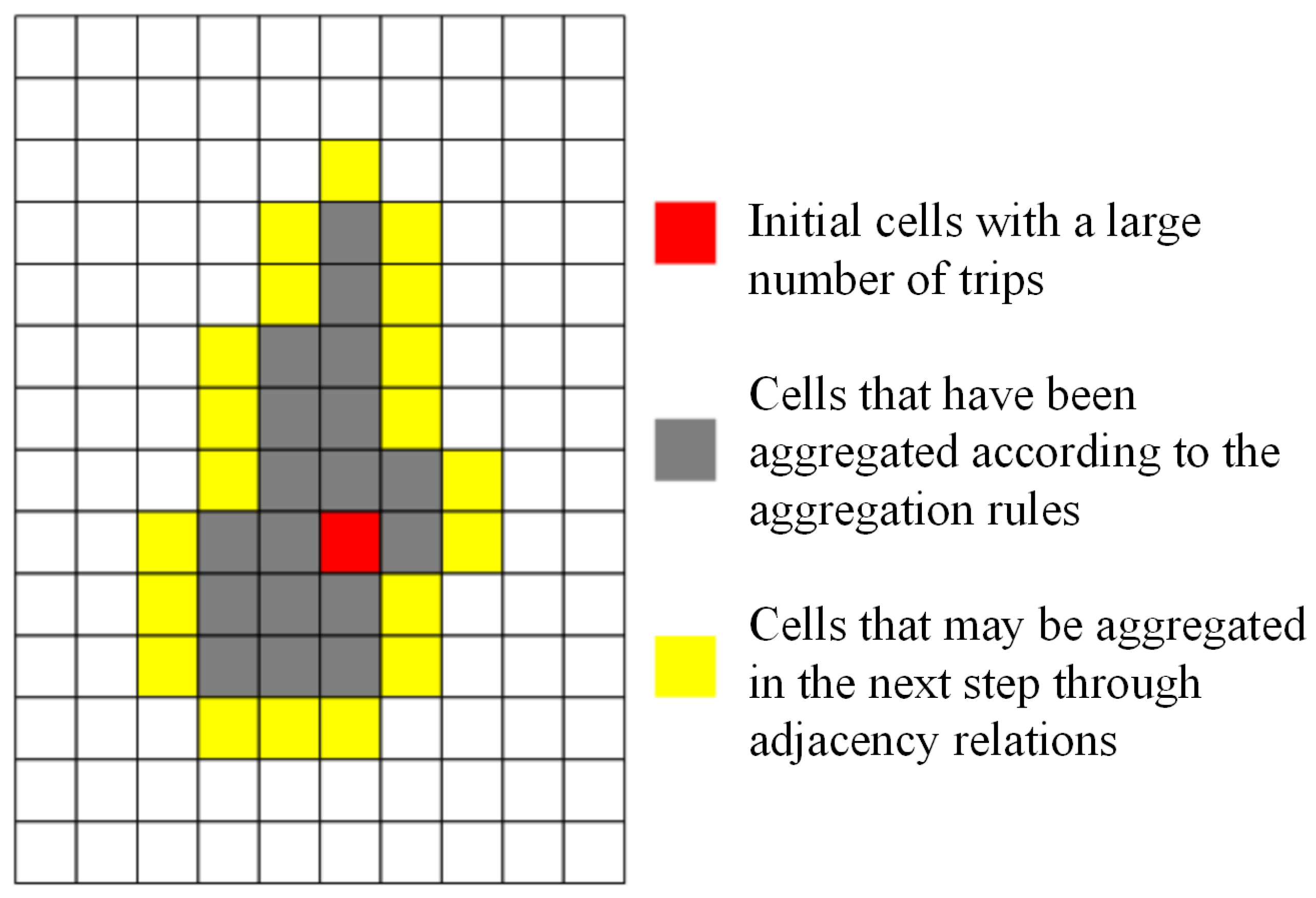
The aggregation of each traffic zone starts from the local highest peak, which is defined as follows: According to the total travel volume corresponding to all of the cells obtained above, from large to small, the first N grids are selected as the local highest peak of the aggregated N traffic zones, such as the green cell in Figure 4, also known as the initial cells; then, according to the adjacency relationship between the cells (where edge adjacency is considered to represent the adjacency relationship), the cells that can be aggregated to the aggregated cells (yellow cells in Figure 4) are determined. Then, the cells found through the adjacency relationship are preliminarily screened according to the preliminary screening conditions (Section 3.1), and the objective functions are calculated one by one for each cell that meets the screening conditions to determine the cells that can finally be aggregated to the traffic zone. Finally, judgment of adherence to the constraint condition is carried out. If the constraint condition is not satisfied, the aggregation of the next cell will continue. If the constraint condition is satisfied, aggregation of the next traffic zone will be carried out.
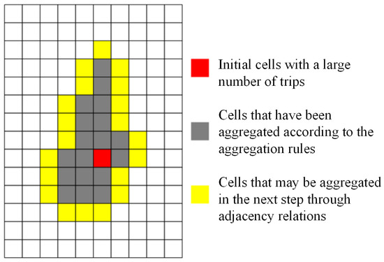
Figure 4.
Aggregation rules for single traffic analysis zone.
3.1. Preliminary Screening Conditions of Polymerization Unit
In order to ensure that the shape of the formed traffic zone remains regular, that the travel in the traffic zone is similar, and that the computational performance of the aggregation model is improved, the grid is preliminarily screened. The screening conditions are as follows:
(1) Distance constraint: The distance between the cell centroid found using the above aggregation rules and the local highest-peak cell centroid cannot exceed 1000 m, which ensures the regularity of the traffic zone and avoids the formation of a concave or narrow traffic zone. It is convenient to simplify the centroid position of the traffic zone in specific practical projects.
(2) Time distribution similarity constraint: Based on the time distribution similarity coefficient between adjacent grids, the similarity coefficient between the grid found using the aggregation rule and the aggregated adjacent grid cannot be less than 0.4, which ensures the similarity of travel within the same traffic community.
3.2. Optimal Modeling of Traffic Cell Segmentation
According to the principle of TAZ division, the proportion of trips within a TAZ and the difference in travel density between TAZs should be as small as possible. Therefore, the optimization of TAZ division in this study is a multiobjective optimization problem. The purpose of the objective function is to minimize the difference between the travel density of each TAZ and the average travel density of the area, and to minimize the proportion of trips within the TAZ, as shown in Equation (12). Based on the spatiotemporal discretized travel data, spatial grid attribute data are constructed for the traffic subdivision model.
In Equation (12), is the average travel density within the area, which can be calculated by Equation (10), is the total trips in the j-th cell, is the area of the j-th cell, K is the total number of cells, and is the proportion of trips in the area when aggregated with the j-th grid.
Travel similarity constraint: Based on the travel time similarity coefficient between cells, the between the cell i to be aggregated and its adjacent cell j must not be lower than the threshold , as shown in Equation (14).
Travel intensity constraint: The final travel intensity in each TAZ should be greater than 70% of the average travel quantity. This can control the statistical accuracy of the TAZ, which ensures the homogeneity of the travel intensity of all TAZs. After each aggregation, a judgment is made regarding whether the requirements are met, and if they are not, the aggregation will continue.
Constraint on the proportion of trips within the TAZ: The travel proportion within each TAZ should be minimal and should not exceed the threshold to avoid excessive travel within some TAZs and loss of geographic accuracy during aggregate analysis.
Constraints on the TAZ area: Too large a TAZ area will increase the proportion of trips in the TAZ, which will cause the loss of geographic information; however, too small a TAZ area will reduce the statistical accuracy of the TAZ and increase the workload in the investigation, analysis, and forecasting. Therefore, in order to ensure balance between the geographic information and statistical accuracy, the area of the TAZ formed should be within a reasonable range, as shown in Equation (17).
Constraint on TAZ shape: In order to ensure that the TAZ is a convex polygon, the inner angle of the polygon formed by the outermost cell centroids is calculated according to the angle discrimination method to determine whether it is less than 180°, as shown in Equation (18).
3.3. Evaluation of Optimization Effect
To select the optimal TAZ division scheme from a series of optimization schemes with different TAZ numbers, three macro-indicators are used to evaluate the overall characteristics of each scheme.
(1) Traffic cell equivalent radius
The traffic cell radius RE is the radius of the equal-area circle for each traffic cell, which is used to describe the geographic accuracy of the divided traffic cell (see Equation (19)).
(2) Traffic cell travel density
The traffic cell travel density is used to calculate the objective function each time the traffic cell cycles through the aggregated grid, and its value is constantly updated (see Equation (20), where and represent the traffic trips and the grid area of the i grid, respectively).
(3) Standard deviation of travel density in traffic neighborhoods
The standard deviation of traffic cell travel density is used to describe the traffic cell aggregation objective function. As far as possible, the traffic cell in the aggregation process is a constant iterative calculation of the value, to ensure the homogeneity of travel within the traffic cell (see Equation (21)).
(4) Coefficient of variation of travel density
This indicator is used to evaluate the homogeneity of the zoning system traffic cell travel density. The larger the value of the indicator, the weaker the homogeneity of the travel density of the traffic cell, reflecting the strengths and weaknesses of the traffic cell program, calculated as shown in Equation (22).
where denotes the average trip intensity of transportation neighborhood i in each scenario.
(5) Average proportion of trips in scheme
According to the travel proportion of each TAZ in the scheme, the arithmetic mean is calculated to obtain the average proportion of trips in the scheme.
Based on the above evaluation indicators, this study adopts the TOPSIS comprehensive evaluation method to analyze all schemes and to obtain the most ideal TAZ division scheme. This method finds the worst plan and the best plan (represented by the worst vector and the best vector, respectively) by normalizing the original data matrix. The distance between the optimal scheme and the worst scheme and all of the evaluation objects is calculated to obtain the proximity between the optimal scheme and all of the evaluation objects. In this way, the merits and disadvantages of all of the evaluation objects are evaluated.
3.4. Solving Traffic Cell Segmentation Model
Based on the constructed TAZ division model, this study optimizes the division scheme using four layers, as shown in Figure 5.
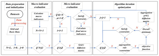
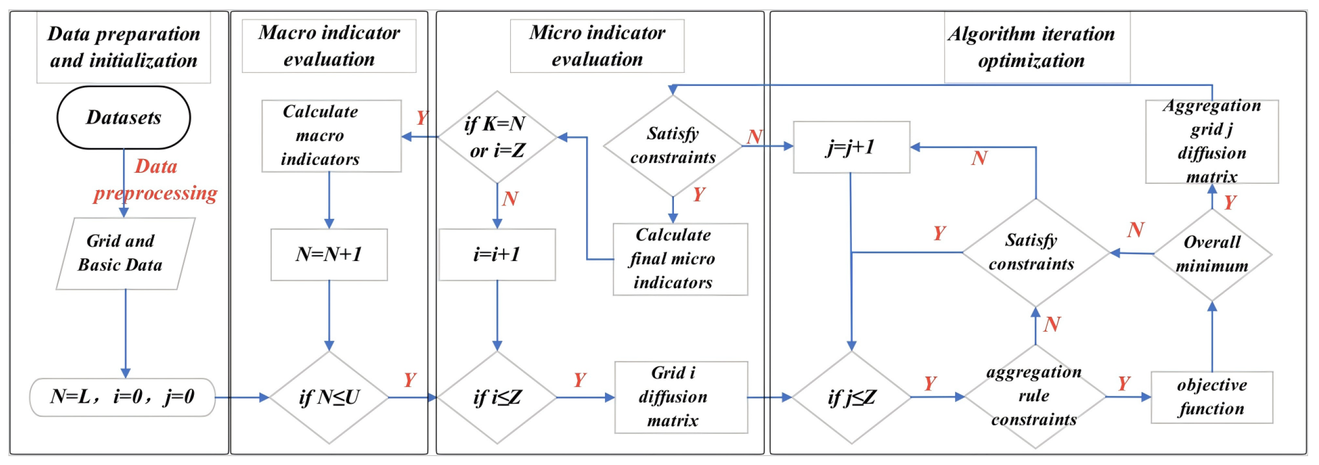
Figure 5.
Structure diagram of the algorithm. Detailed pseudocode is provided in Algorithm 1.
Figure 5.
Structure diagram of the algorithm. Detailed pseudocode is provided in Algorithm 1.
| Algorithm 1: TAZ division scheme and evaluation process. |
 |
The first layer is the data preparation and initialization layer, which preprocesses the original dataset; sets the upper and lower limits of the number of traffic cells , of the number of spatial cells , and of the number of iterative optimization times in the division scheme; and initializes the counts N of the traffic cells, the counts i of the spatial cells, and the counts j of the iterative optimization.
The second layer is the macro-indicator assessment layer. The division scheme starts with the formation of , and after completing a scheme, the macro evaluation indicators of each scheme are calculated; then schemes are divided (where l is the interval between the number of schemes) until the division of schemes is completed, through which division schemes are obtained.
The third layer is the micro-indicator evaluation layer. The starting cell for TAZ division is selected according to the second layer and the travel feature data of spatial cells. The optimal aggregation set of cells in each TAZ is obtained through the scheme formation layer.
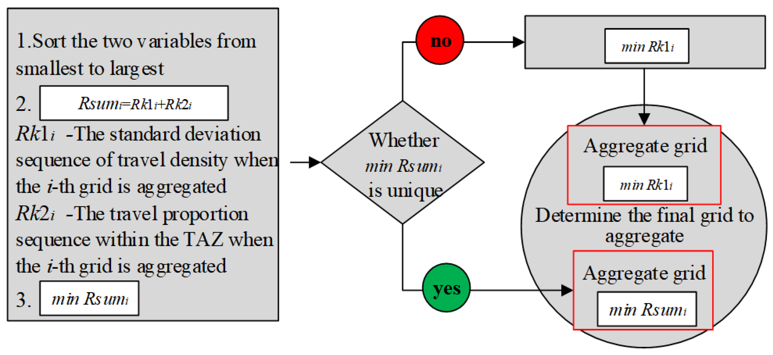
The fourth layer is the iterative optimization layer of the algorithm. In the scheme, the aggregation of each TAZ starts from the starting cell, and a scheme is generated according to the aggregation optimization model. Scheme formation is a multiobjective optimization process that needs to minimize the travel density difference and travel proportion in each cell. During scheme formation, these two variables are calculated after the cell found based on the aggregation rules is singled out by constraints. Then, the two variables are sorted from smallest to largest to calculate their algebraic sum. If the i grid meets both the standard deviation of travel density and the minimum travel proportion, the i grid is aggregated. If the sequence sum is not unique, then grid i with the smallest standard deviation of travel density is aggregated, as shown in Figure 6.
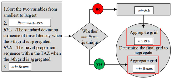
Figure 6.
A flow chart depicting the process of determining the optimal aggregation grid. The chart illustrates the step-by-step process of selecting the optimal aggregation grid, starting from the initial data and proceeding through the calculation of the distances between each grid and the ideal solutions. Rsumi: The sum of distances between each aggregation grid’s characteristics and the ideal solution. Rk1i and Rk2i: The distances between the k-th grid aggregation scheme and the first and second ideal reference solutions, respectively. minRsumi: The minimum value of Rsumi across all aggregation schemes, indicating the optimal aggregation grid. The flow chart details the iterative process of selecting the best grid aggregation scheme based on these calculated distances.
3.5. Programmatic Refinements
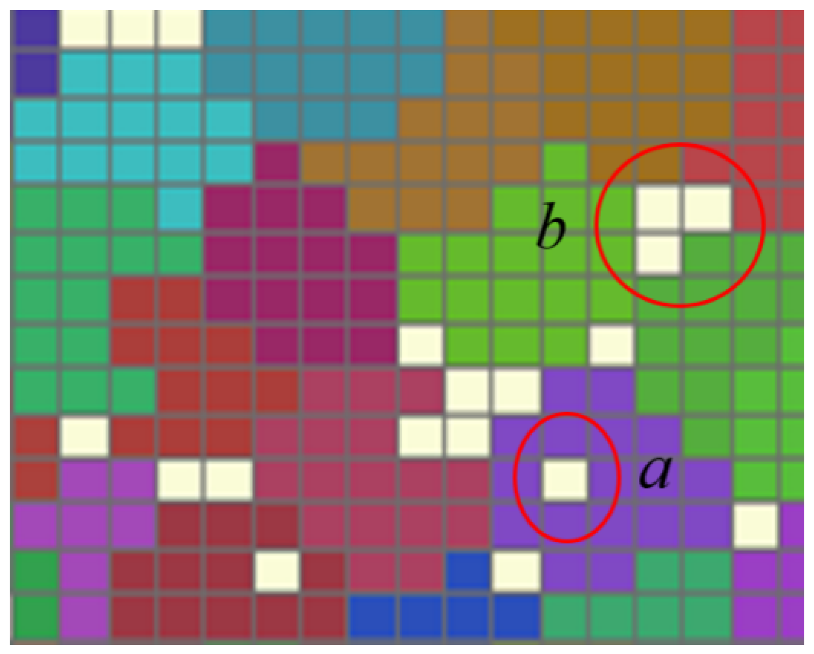
After the optimization model calculation, most of the cells will be aggregated to form multiple traffic cell scenarios according to the given range. However, there are still some grids that are not aggregated, which can be divided into the following two cases according to their locations: (1) located inside the traffic cell, such as region a in Figure 7, and (2) located at the boundary of the traffic cell, such as region b in Figure 7.
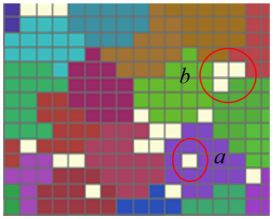
Figure 7.
Unaggregated grids in the aggregation model.
For the first type of grid (region a), according to the TAZ division principle, there should be no TAZs with a concave polygonal shape. Thus, the unaggregated grids only need to be aggregated to the corresponding TAZ. As for the second type, the number of adjacent edges between unaggregated grids and adjacent TAZs is counted according to the adjacency relation between grids and aggregated to the TAZ with the largest number of adjacent edges, so that there are no concave polygonal TAZs. If the number of adjacent edges is the same, the area of adjacent TAZs is calculated and aggregated into TAZs with a small area to ensure the homogeneity of TAZs. Finally, a TAZ division scheme with clear boundaries is formed.
4. Case Validation and Analysis
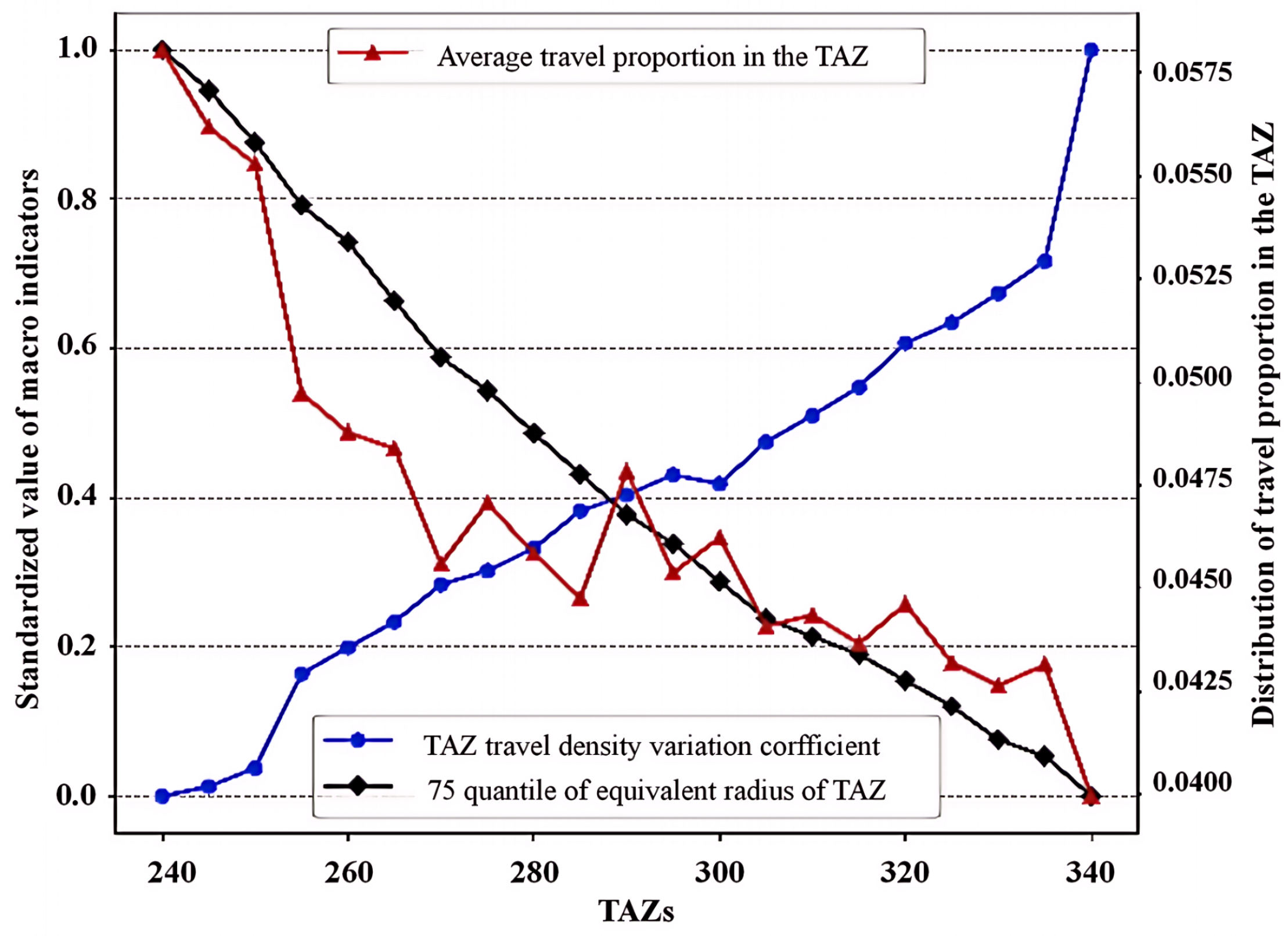
Based on the constructed TAZ aggregation model, the TAZ within the Fourth Ring Road in Beijing was delineated using GIS data of the bus network and bus card data collected on a working day in March 2016. During the delineation process, the number of TAZs was varied between 240 and 340, with an increment of five TAZs per scheme, resulting in a total of 21 different TAZ delineation schemes. Figure 8 illustrates the changes in macro-indicators for each scheme.

Figure 8.
Macro-indicators of the TAZ scheme.
As the number of TAZs increases, the area of each TAZ decreases, and the proportion of trips within each TAZ shows a decreasing trend. Moreover, the average trip proportion within each area remains below 10%, and the variation coefficient of travel density decreases. When the number of TAZs is around 285 to 290, these indicators reach a relative balance. To evaluate and select the optimal TAZ delineation scheme, the macro-indicator matrix for all schemes was calculated, with the results shown in Table 1, and the proximity of each scheme to the ideal solution was determined using the TOPSIS (Technique for Order Preference by Similarity to Ideal Solution) evaluation method, as shown in Table 2.

Table 1.
Normalized matrix of macro-indicators.
Table 2.
The proximity of TAZ schemes to the optimal scheme.
In Table 1, the normalized macro-indicator matrix for all TAZ delineation schemes is presented. This matrix includes the key performance indicators for each scheme, such as the area of each TAZ, the trip proportion within each TAZ, and the travel density variation coefficient. These values were normalized to ensure they could be compared on the same scale across different TAZ schemes. Table 2 shows the proximity of each scheme to the ideal solution, calculated using the TOPSIS method. The proximity value reflects how close each scheme is to the ideal solution, with higher values indicating better overall performance. The scheme with the highest proximity value (285 TAZs) was selected as the optimal delineation scheme for this study.
TOPSIS, proposed by Hwang and Yoon in 1981 [29], is a widely used method for multicriteria decision analysis. The method begins by normalizing the original data matrix and determining the ideal and worst solutions (represented by the ideal and worst vectors). The proximity of each evaluation object to the ideal solution is calculated by measuring the Euclidean distance to both the ideal and worst solutions. This method is commonly used to select the best solution based on its closeness to the ideal solution and its distance from the worst solution.
The results indicate that when the number of TAZs is 285, the proximity to the ideal solution is the highest, yielding the best TAZ delineation effect. When the number of TAZs is too large or too small, the proximity is lower, indicating poorer overall performance. Therefore, 285 TAZs were selected as the optimal TAZ delineation scheme for the area within Beijing’s Fourth Ring Road.
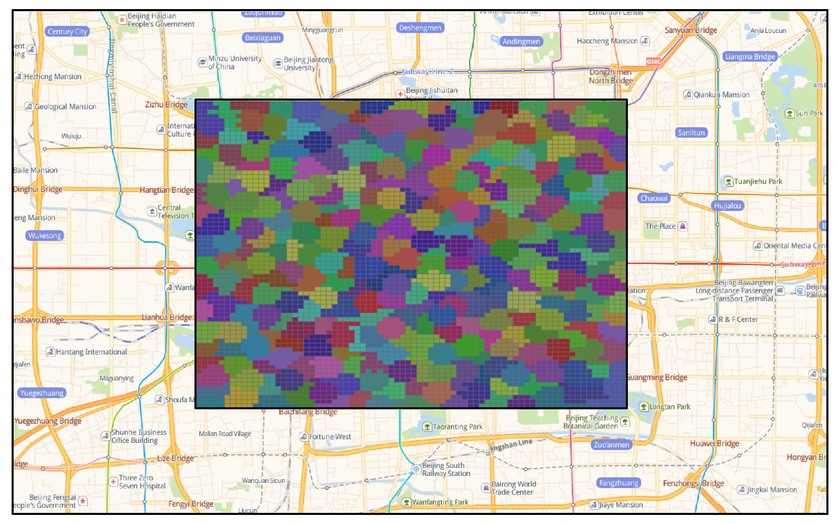
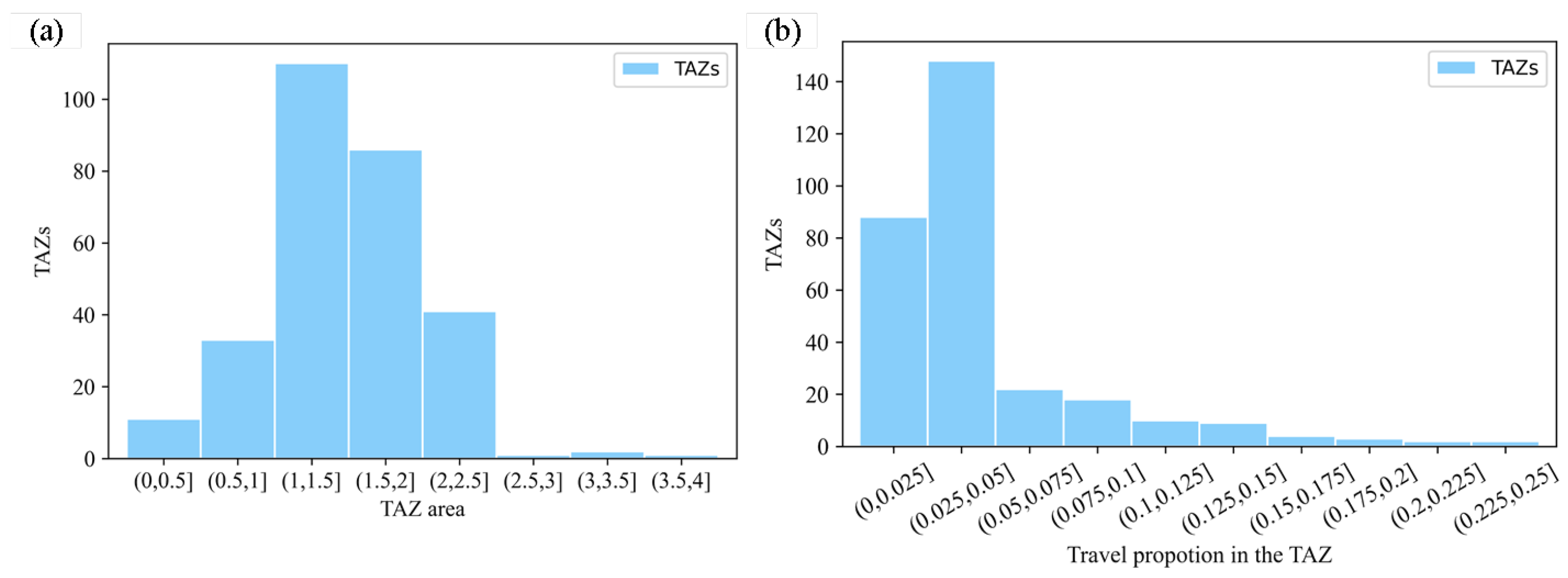
By applying the TOPSIS comprehensive evaluation method, the optimal number of traffic districts within the Fourth Ring Road area of Beijing was determined to be 285, with the division results shown in Figure 9, where different colors represent different traffic districts. The distribution of the areas of all traffic districts when the study area was divided into 285 traffic districts is shown in Figure 10a. The areas are primarily distributed within the range of [0.5 km2, 2.5 km2], accounting for more than 95% of the total number of traffic districts. Traffic districts with an area larger than 2.5 km2 resulted from the re-aggregation of grids that had not been previously aggregated, which caused the areas of some traffic districts to exceed the above range. Traffic districts with an area smaller than or equal to 0.5 km2 occurred because during the aggregation process, grids adjacent to already aggregated areas were merged into other traffic districts, forcing the aggregation process to terminate prematurely. Based on the final traffic district division scheme, the bus station OD matrix, and the travel volume corresponding to each grid, the travel proportion within the optimal traffic district division scheme was determined and is shown in Figure 10a. The analysis indicates that more than 90% of the traffic districts have a travel proportion of less than 15%, ensuring minimal loss of travel information during the division of traffic districts.
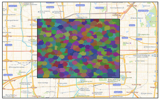
Figure 9.
The optimal Traffic Analysis Zone division scheme (285 TAZs). In this figure, each colored region represents a distinct TAZ. The color coding indicates different TAZs, with the optimal division scheme consisting of 285 TAZs. The boundary lines are based on GIS data and bus network information from March 2016.
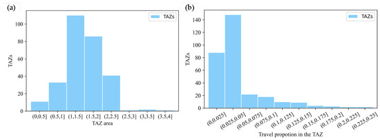
Figure 10.
Distribution of micro-indicators of optimal TAZ division scheme; (a) distribution of TAZ area; (b) distribution of travel proportion in TAZ.
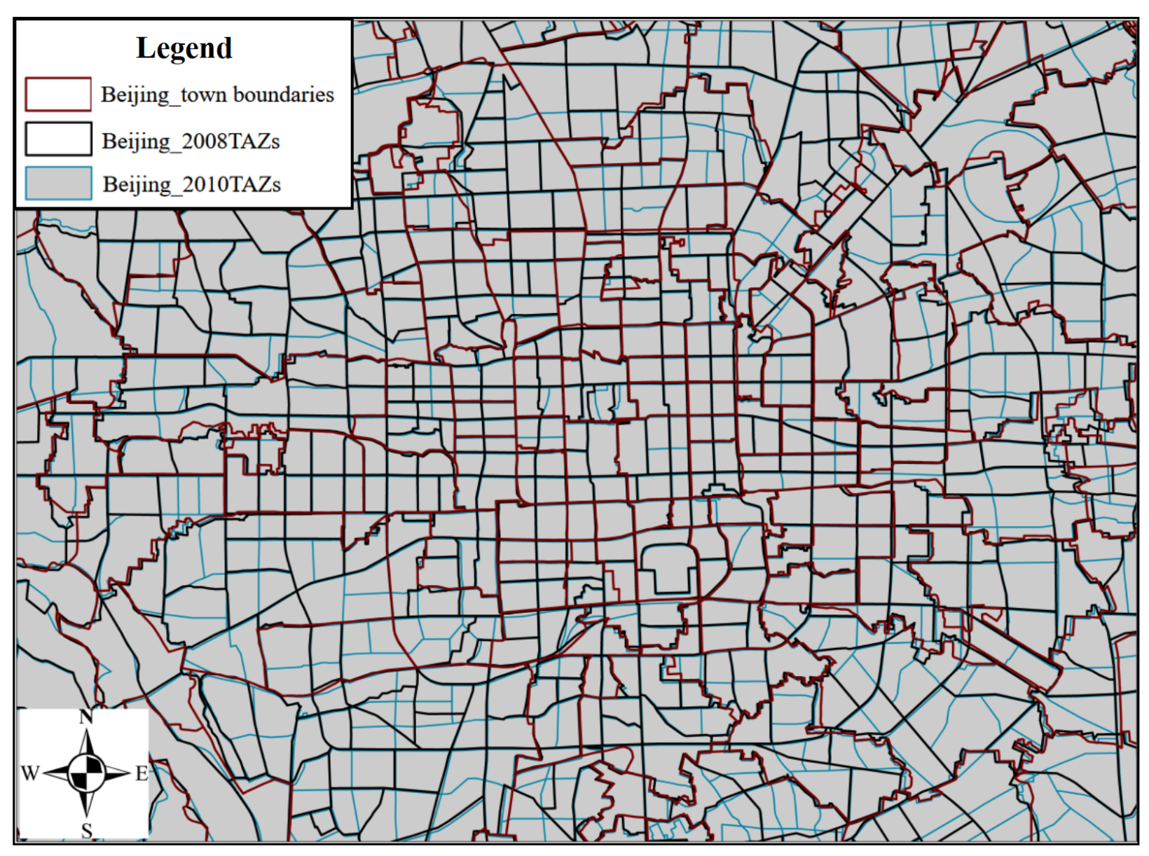
To further verify the reliability and effectiveness of the TAZ division method proposed in this study, our scheme was compared with the Beijing 2008 and 2010 TAZs. Figure 11 shows the boundaries of townships in Beijing and the boundaries of TAZs in 2008 and 2010. By comparing the three types of boundaries, it was found that the TAZs in 2008 were mostly subdivided on the basis of administrative divisions, while those in 2010 were subdivided based on the 2008 TAZs. Based on the macroscopic evaluation indexes of traffic subdivisions, systematic calculations were carried out for each subdistrict, and the calculation results are shown in Table 3. The traffic cell program proposed in this study further reduces the proportion of trips in the average area to avoid the loss of travel information; the coefficient of variation of travel density is lower than the corresponding value of the traffic cell program in 2008 and 2010 to ensure the homogeneity of traffic cell trips. It can be seen that in 2008 and 2010, the traffic district meets the traffic district boundaries and administrative boundaries, making it compatible with the principle of easy access to socioeconomic, demographic, and employment data in traffic planning and traffic modeling, but it is difficult to ensure the accuracy of the traffic district program based on the relevant predictive analysis.
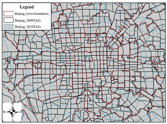
Figure 11.
Comparison of different partition boundaries.
Table 3.
Comparison of indicators of TAZ division schemes.
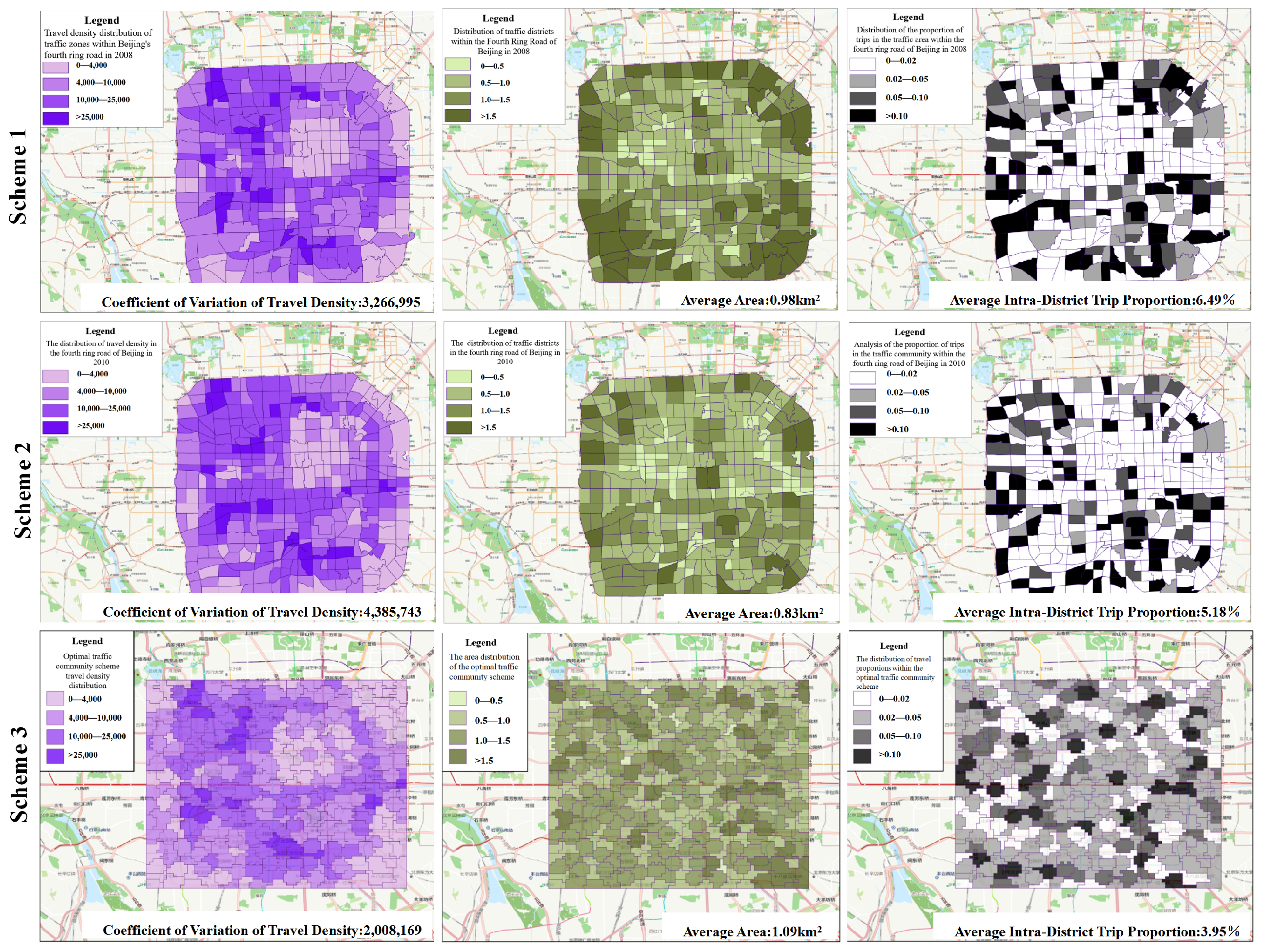
It can be seen from the spatial distribution in Figure 12 that the proposed scheme significantly reduces the number of TAZs with a travel proportion of over 10%, indicating an even travel proportion distribution. Furthermore, in the 2008 TAZ scheme, the travel proportion is as high as 40%. This figure is only 22% in the proposed scheme, in which the TAZ area and travel density are more evenly distributed.
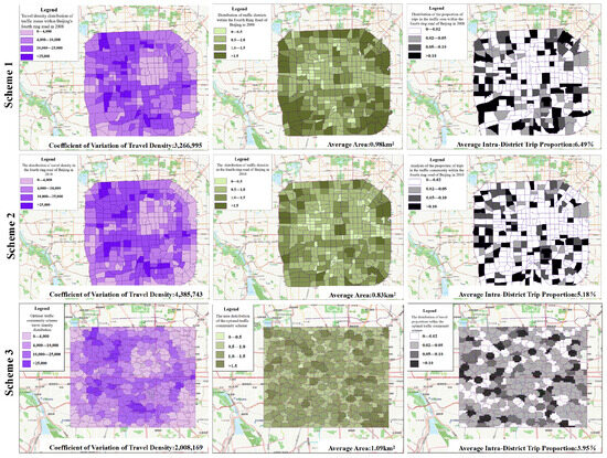
Figure 12.
Micro indicators in different Traffic Analysis Zone schemes. This figure presents the distribution of key macro-indicators for three different Traffic Analysis Zone schemes across nine subplots.
5. Conclusions
Based on a comprehensive review of studies related to transit card data and traffic zone division, this study utilizes transit card data within Beijing’s Fourth Ring Road to construct a traffic zone aggregation model following relevant traffic zone division guidelines. Subsequently, the traffic zones within the study area are delineated, and the optimal traffic zone division scheme is selected, compared with other traffic zone schemes, and verified to reflect the actual travel behavior of residents. Our research findings and conclusions are as follows:
(1) Preprocessing of transit card data and development of matching and integration methodology. In this study, we conducted preprocessing of transit card data and designed a matching and integration methodology for the data. Based on a detailed description of both transit card data and transit network GIS data, several rules were proposed to preprocess the data, ensuring data quality during application. To address mismatches between transit card data and transit network GIS data, field surveys were conducted to collect bus stop sign information, which was used to match the two datasets. Additionally, bus stops with identical codes on the same route, as well as stops with the same name but located on different routes or in close proximity, were integrated. This methodology is of significant importance for analyses based on transit card data.
(2) Construction of traffic zone aggregation model based on travel similarity. Drawing on prior research on traffic zone division and guided by the principles of traffic zone division, a traffic zone aggregation objective function and constraints were developed to construct a traffic zone aggregation model. Using the area within Beijing’s Fourth Ring Road as the study area, the model generated 21 traffic zone division schemes, with the number of traffic zones ranging from a minimum of 240 to a maximum of 340.
(3) Selection of optimal traffic zone scheme based on TOPSIS comprehensive evaluation method and comparative analysis. The optimal traffic zone scheme was selected from the 21 schemes using the TOPSIS (Technique for Order of Preference by Similarity to Ideal Solution) comprehensive evaluation method, and it was compared with Beijing’s traffic zone division plans from 2008 and 2010. The results demonstrate that the traffic zone division scheme based on the aggregation model offers certain advantages. The optimal traffic zone scheme includes 285 zones, with each zone’s area generally falling within the range of [0.5 km2, 2.5 km2]. The proportion of intrazonal travel in the optimal scheme remains below 15% overall and is superior to that in the 2008 and 2010 traffic zone division schemes. This indicates that the optimal scheme better reflects the actual travel behavior of residents.
Based on Beijing bus card data and bus network GIS data, a traffic zone aggregation model was constructed in this study to divide the traffic zone in the fourth ring area, and the traffic zone division method was optimized to a certain extent. However, in order to place the model into practice, there are still some problems to be solved:
(1) The method of traffic zone division used in this study was based on the principle of relevant zone division. Regarding the data used in this study, they are only considered in terms of the homogeneity, information loss, area, and shape of the traffic zone. The division of the traffic zone under other relevant principles needs to be discussed further.
(2) Restricted by personal privacy and relevant laws and regulations, only the bus card data were considered in the model construction process. In the future, when passengers’ travel information is more transparent, more comprehensive multimodal data should be considered.
(3) With the development of society, the travel mode of residents will change considerably. In the future, we should more closely combine actual passenger flow forecasting and other projects, and update the plan according to the specific application scenario.
Author Contributions
Conceptualization, K.D. and J.S.; Formal analysis, D.C. and Y.Z.; Methodology, J.S.; Resources, K.D. and Y.Z.; Supervision, J.S.; Validation, D.C.; Writing—original draft preparation, K.D.; Writing—review and editing, K.D., J.S., D.C. and Y.Z.; Visualization, D.C. and M.L.; Project administration, M.L. and Y.Z.; Funding acquisition, K.D. and J.S. All authors have read and agreed to the published version of the manuscript.
Funding
This research was funded by Shaanxi Provincial Qinchuangyuan’s ‘Scientist + Engineer’ Team Construction grant number 2022KXJ-022, National Natural Science Foundation of China, grant number 52202385.
Institutional Review Board Statement
Not applicable.
Informed Consent Statement
Not applicable.
Data Availability Statement
The original contributions presented in this study are included in the article. Further inquiries can be directed to the corresponding author.
Acknowledgments
We would like to express our sincere gratitude to Xianwu Gong from Chang’an University for his invaluable guidance and support throughout the development of this thesis.
Conflicts of Interest
The authors declare no conflicts of interest.
References
- Ghadiri, M.; Rassafi, A.A.; Mirbaha, B. The effects of traffic zoning with regular geometric shapes on the precision of trip production models. J. Transp. Geogr. 2019, 78, 150–159. [Google Scholar] [CrossRef]
- Hosseinzadeh, A.; Algomaiah, M.; Kluger, R.; Li, Z. Spatial analysis of shared e-scooter trips. J. Transp. Geogr. 2021, 92, 103016. [Google Scholar] [CrossRef]
- Mirzahossein, H.; Bakhtiari, A.R.; Kalantari, N.T.; Jin, X. Investigating mandatory and non-mandatory trip patterns based on socioeconomic characteristics and traffic analysis zone features using deep neural networks. Comput. Urban Sci. 2022, 2, 35. [Google Scholar] [CrossRef]
- Li, H.; Wu, D.; Zhang, Z.; Zhang, Y. Safety impacts of the discrepancies and accesses between adjacent traffic analysis zones. J. Transp. Saf. Secur. 2020, 14, 359–381. [Google Scholar] [CrossRef]
- Briz-Redón, A.; Martínez-Ruiz, F.; Montes, F. Investigation of the consequences of the modifiable areal unit problem in macroscopic traffic safety analysis: A case study accounting for scale and zoning. Accid. Anal. Prev. 2019, 132, 105276. [Google Scholar] [CrossRef] [PubMed]
- Guo, C. Suggestions on the Optimization and Application of Traffic District Division Scheme of National Railway Transportation Network; Research on Railway Economy: Beijing, China, 2019; pp. 1–5. [Google Scholar]
- Yang, B.; Tian, Y.; Wang, J.; Hu, X.; An, S. How to improve urban transportation planning in big data era? A practice in the study of traffic analysis zone delineation. Transp. Policy 2022, 127, 1–14. [Google Scholar] [CrossRef]
- Rahman, M.S.; Abdel-Aty, M.; Hasan, S.; Cai, Q. Applying machine learning approaches to analyze the vulnerable road-users’ crashes at statewide traffic analysis zones. J. Saf. Res. 2019, 70, 275–288. [Google Scholar] [CrossRef] [PubMed]
- Wang, X.; Zhou, Q.; Yang, J.; You, S.; Song, Y.; Xue, M. Macro-level traffic safety analysis in Shanghai, China. Accid. Anal. Prev. 2019, 125, 249–256. [Google Scholar] [CrossRef]
- Sahu, P.K.; Aitichya Chandra, A.P.; Majumdar, B.B. Designing freight traffic analysis zones for metropolitan areas: Identification of optimal scale for macro-level freight travel analysis. Transp. Plan. Technol. 2020, 43, 620–637. [Google Scholar] [CrossRef]
- Moghaddam, S.; Ameli, M.; Rao, K.R.; Tiwari, G. Delineation of Traffic Analysis Zone for Public Transportation OD Matrix Estimation Based on Socio-spatial Practices. In Proceedings of the 4th Symposium on Management of Future Motorway and Urban Traffic Systems 2022 (MFTS2022), Dresden, Germany, 30 November–2 December 2022; pp. 205–2016. [Google Scholar] [CrossRef]
- Zhao, H.; Zhou, Y. Traffic Analysis Zones: How Do We Move Forward? In Applying Census Data for Transportation; TRB: Washington, DC, USA, 2017; p. 67. [Google Scholar]
- Miller, E. Traffic Analysis Zone Definition: Issues & Guidance; Travel Modeling Group, Transport Research Institute, University of Toronto: Toronto, ON, Canada, 2021. [Google Scholar]
- Lian, J.; Li, Y.; Huang, S.L.; Zhang, L. Mining mobility patterns with trip-based traffic analysis zones: A deep feature embedding approach. In Proceedings of the 2019 IEEE Intelligent Transportation Systems Conference (ITSC), Auckland, New Zealand, 27–30 October 2019; pp. 1650–1657. [Google Scholar]
- Castiglione, M.; Nigro, M.; Sacco, N. Multi-source Data-driven Procedure for Traffic Analysis Zones Definition. In Proceedings of the 2023 8th International Conference on Models and Technologies for Intelligent Transportation Systems (MT-ITS), Nice, France, 14–16 June 2023; pp. 1–6. [Google Scholar]
- Zhang, X.; Zhang, N. Dynamic OD extraction method of motor vehicles in traffic zones based on LPR and POI data. Integr. Transp. 2023, 45, 96–101. [Google Scholar]
- Gao, Y.; Liao, Y. Urban Tourism Traffic Analysis Zone Division Based on Floating Car Data. Promet-Traffic Transp. 2023, 35, 395–406. [Google Scholar] [CrossRef]
- Wang, X.Q.; Zhao, C.F.; Yin, C.Y.; Dong, C.J. Research on car ownership behavior considering the correlation of traffic zones. Transp. Syst. Eng. Inf. 2019, 19, 28–32+71. [Google Scholar] [CrossRef]
- Wu, D.; Ma, L.; Yan, X. Applying and Evaluating Data-Driven Fine Grid Partitioning Methods for Traffic Analysis Zones. J. Urban Plan. Dev. 2024, 150, 04024004. [Google Scholar] [CrossRef]
- Obelheiro, M.R.; da Silva, A.R.; Nodari, C.T.; Cybis, H.B.B.; Lindau, L.A. A new zone system to analyze the spatial relationships between the built environment and traffic safety. J. Transp. Geogr. 2020, 84, 102699. [Google Scholar] [CrossRef]
- Yao, H.; Chen, D. Comparison of apportionment methods for assigning trip data to rezoned traffic analysis zones: A case study of Toronto, Canada. Can. Geogr. Géographe Can. 2021, 65, 321–332. [Google Scholar] [CrossRef]
- Song, L.J.; Zhu, J.Z.; Liu, X.J.; Chen, J.; Xian, K. Optimization Method of Traffic Analysis Zones Division in Public Transit Corridor. J. Transp. Syst. Eng. Inf. Technol. 2020, 20, 34. [Google Scholar]
- Wang, J.; Gao, J.J. Urban traffic zone division based on DBSCAN algorithm. Smart City 2023, 9, 80–82. [Google Scholar] [CrossRef]
- Beijing Transportation Development & Research Center. The Fifth Comprehensive Traffic Survey Report of Beijing; Beijing Transportation Development & Research Center: Beijing, China, 2016. [Google Scholar]
- Yang, B.Y. Research on Traffic Zone Division Method Based on Multi-Source Data. Master’s Thesis, Harbin Polytechnic Institute, Harbin, China, 2020. [Google Scholar]
- Zhou, X.; Sun, C.; Niu, X.; Shi, C. The modifiable areal unit problem in the relationship between jobs–housing balance and commuting distance through big and traditional data. Travel Behav. Soc. 2022, 26, 270–278. [Google Scholar] [CrossRef]
- Amoh-Gyimah, R.; Saberi, M.; Sarvi, M. The effect of variations in spatial units on unobserved heterogeneity in macroscopic crash models. Anal. Methods Accid. Res. 2017, 13, 28–51. [Google Scholar] [CrossRef]
- Yue, Z.H. Optimization of Transfer Station Between Urban Rail Transit and Conventional Bus Based on Credit Card Data. Master’s Thesis, Beijing Jiaotong University, Beijing, China, 2017. [Google Scholar]
- Hwang, C.L.; Yoon, K. Multiple Attribute Decision Making: Methods and Applications—A State-of-the-Art Survey; Lecture Notes in Economics and Mathematical Systems; CRC Press: Boca Raton, FL, USA, 1981. [Google Scholar]

Disclaimer/Publisher’s Note: The statements, opinions and data contained in all publications are solely those of the individual author(s) and contributor(s) and not of MDPI and/or the editor(s). MDPI and/or the editor(s) disclaim responsibility for any injury to people or property resulting from any ideas, methods, instructions or products referred to in the content. |
© 2024 by the authors. Licensee MDPI, Basel, Switzerland. This article is an open access article distributed under the terms and conditions of the Creative Commons Attribution (CC BY) license (https://creativecommons.org/licenses/by/4.0/).