Abstract
This article presents a non-destructive method, based on the response to free vibrations, which can be used with efficiency and reliability to determine the Young’s modulus of polymer composite materials reinforced with natural or synthetic fibers. The non-destructive tests are carried out by measuring the frequencies of bending free vibrations of cantilever beams with additional masses. By using inverse methods, the experimental values of elasticity modulus E are assessed and validated by numerical simulation, using the finite element method (FEM). For FEM modeling, the materials are considered linear, homogeneous, isotropic, and viscoelastic.
1. Introduction
In recent years, because of the sustainability goals identified at a public policy level, composites with natural fibers, alongside synthetic fibers, have gained an increased use in both structural and non-structural applications. Some of these applications, which include a large variety of products, are in furniture manufacturing. Thus, the challenge for producers resides in designing, characterizing, and testing new composite materials in a robust and reliable manner. While the general approach in determining the viscoelastic mechanical properties of composite materials has been to perform destructive tests on a relatively large number of samples, novel non-destructive testing (NDT) methods have been developed in order to reduce the time needed to characterize them and to improve the quality assurance of fabrication [1,2,3]. Non-destructive testing is the process of testing and inspecting materials that causes no physical damage to the testing object, keeping it in its current state [4].
Various NDT methods built upon different principles for quality assurance during the whole lifecycle of the composite products are presented in papers [5,6]. As the composite materials with natural fibers are usually non-homogeneous and anisotropic, their elasticity constants should be viewed as global parameters of the tested samples or structures. The evolution of the defects and damages, which can occur within numerous locations at various levels of scale (from nano to macro), is difficult to track by performing only destructive testing.
A very efficient method for testing the structural degradation and fatigue behavior of composite materials and structures is the vibration resonance method [7]. Damage alters the modal properties such as natural frequencies, mode shapes, and damping ratios [8,9,10]. Various optimized inverse methods have been developed for damage identification in structures based on the stiffness separation method for reducing calculation time [11,12,13].
The elastic modulus is a key parameter in engineering design of structures and material development. The bending vibration frequencies are primarily controlled by the Young’s modulus of the tested specimen, being practically independent of any material anisotropy. The dynamic determination of the flexural elastic modulus E of strawboards using NDT methods based on the free plate modal or transient excitation test is presented in paper [14].
The impulse excitation technique is a non-destructive material characterization method used to determine the elastic properties and internal friction of a material of interest [15]. The test can be carried out by using material samples (light beams or plates) with or without small additional masses (i.e., accelerometers for measuring the transient response). These masses should be placed such as to enhance the load stress in tested specimens, produced by free vibration modes, excited by force impact or initially imposed displacements [16,17]. Using the free vibration excitation by imposing an initial deformation (potential energy) at the free end of tested sample, followed by a sudden release, is very convenient for both testing (easy to control) and modeling (introduced as initial condition for the equation of motion).
In correlation with this, many papers explore numerical methods for determining the eigenfrequencies of composite material samples with simple geometries, based on the elastic constants of the materials treated as homogenized and macroscopically uniform [18,19,20,21].
Nonetheless, some of the limitations of the referenced studies include complex material definitions, a lack of experimental validation, cumbersome analytical expressions, or imply highly specialized personnel in a potential production compliancy sector.
The objective of this work is to determine the values of the material constant for composite materials (polymer reinforced with natural fibers), without taking into account the material constants of neither the constituent elements nor their proportions [22]. The proposed NDT is a generalized inverse method that can be applied for many composite materials, including those with synthetic fibers or hybrid fiber–matrix systems. The current study is focused on composite materials made of polypropylene reinforced with short natural fibers, not on highly directional composite materials which can in fact exhibit significant anisotropy due to fiber orientation and matrix inhomogeneity.
The purpose of the numerical simulation in the present paper, using the finite element method (FEM), is to validate the experimental method, which helped determine the value of the elastic constant E of the composite materials, obtained with the method of the first resonance. The novelty is that, in addition to the resonance method used in the experiments, a method of identification (inverse method) of the value of E is used from the coefficients of the equilibrium equations of the elastic bar that model the transverse vibrations. The materials are treated as homogeneous and isotropic. The numerical solution of the elasto-dynamic equations given by Navier–Cauchy, approximated with finite elements, comes to validate the experimental method, because with the values of the material constants obtained experimentally, a close value of the first resonance frequency calculated with the modal analysis method is obtained, as in the case of experimentally obtained values.
The proposed NDT method remains valid under different environmental conditions, as long as the initial study hypotheses are respected, i.e., the material displays a linear elastic behavior [23,24].
The advantage of this method is that it requires non-expensive laboratory equipment and can be used not only for rapid assessing of the value of Young’s modulus for different composite materials, but also for ensuring rapid fabrication and design, manufacturing conformity, and lowering production costs.
2. Materials and Methods
2.1. Experimental Testing
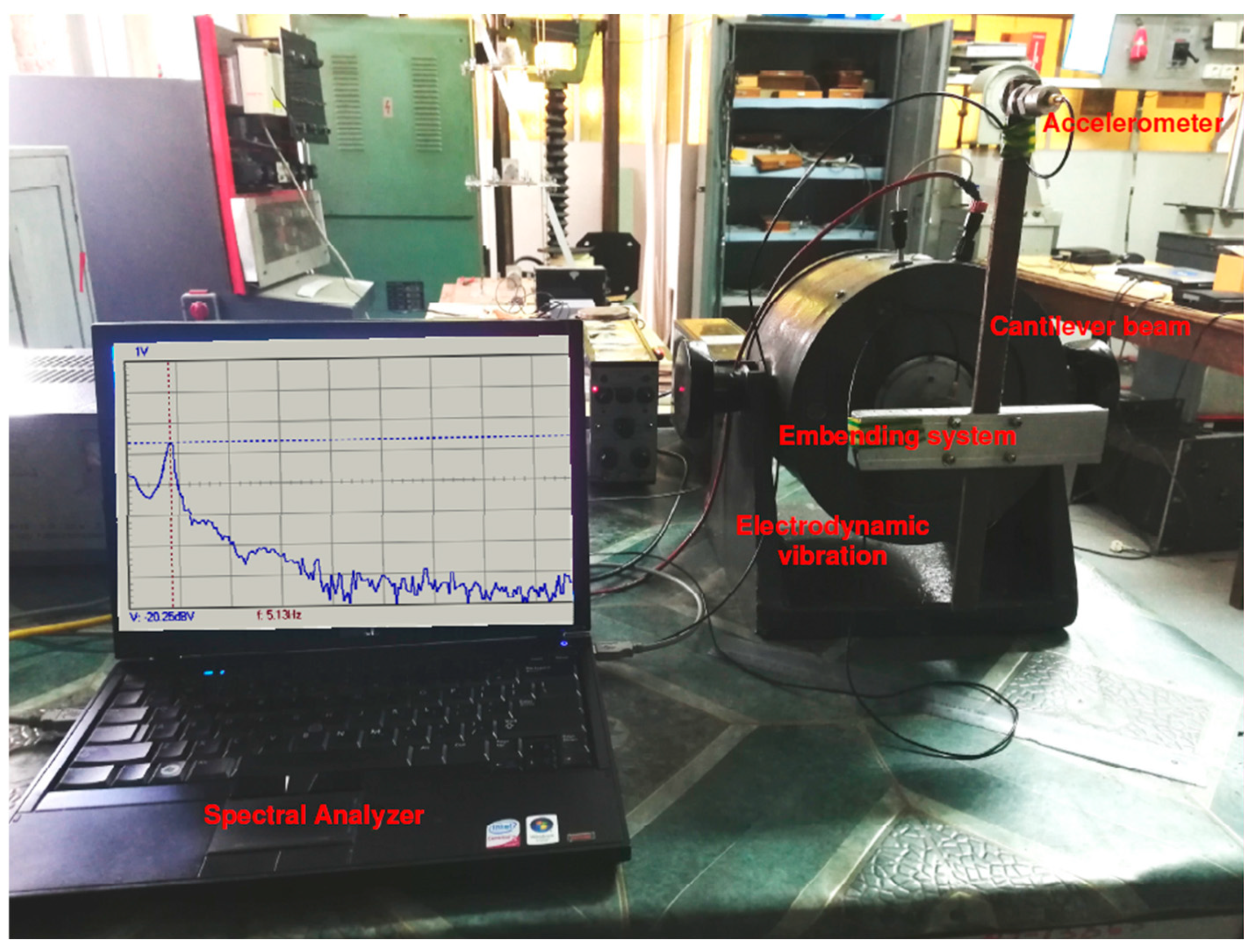
The analyzed composite materials are made from polypropylene resin reinforced with short randomly oriented natural fibers with a relatively uniform arrangement in the fabrication process of furniture plates. The experiments were conducted on two types of slender cantilever beams with rectangular cross sections, made from composite materials: one from polypropylene reinforced with hemp and one from polypropylene with coconut fibers. In order to record the vibration response, a B&K accelerometer was mounted at the free end of the tested sample. This assembly is considered as a single degree of freedom mass-spring system with linear viscoelastic characteristics.
To obtain the bending free vibrations, the tests were performed by imposing an initial displacement at the free end of the cantilever beam. The experimental setup and its schematic are shown in Figure 1 and Figure 2.
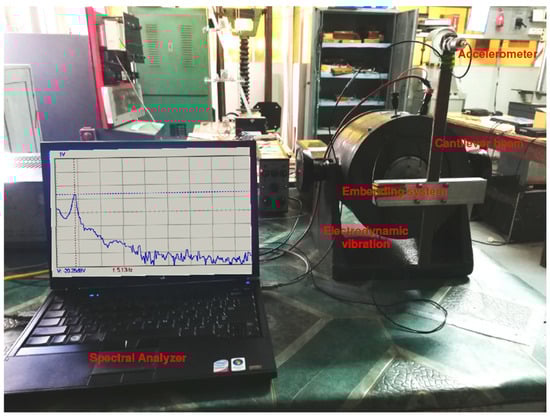
Figure 1.
Experimental setup.
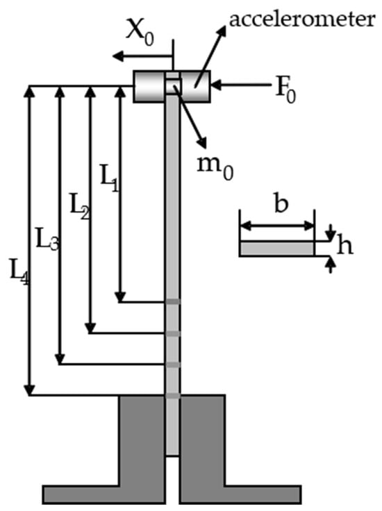
Figure 2.
Schematic of the experimental setup.
For both cantilever beams with hemp and coconut fibers, the following dimensional values were considered: , , , , , . Since there are no European norms on conducting nondestructive tests for determining the Young’s modulus for composite materials reinforced with natural fibers, the authors have chosen specimen dimensions based on the fabrication thickness of the provided furniture plates and on the ratio of slender beams that follow the Euler–Bernoulli beam theory. Moreover, given the selected dimensions, the expected free vibration signals are within the low frequency range in order to reduce the errors associated with high sampling rates.
2.2. Analytical Model
The equation of motion with initial displacement is as follows:
where represents the accelerometer’s mass, the damping coefficients and the stiffness coefficients for a cantilever beam with lengths ; are the displacement, velocity, and the recorded acceleration of the mass , respectively.
where E is the Young’s modulus, and
is the second moment of cross-section area, the width, and the thickness of the beam.
The damped frequencies can be measured from FFT spectra, as well as from the pseudo-periods of free vibration time records for cantilever lengths .
The relative damping coefficients (damping ratios) of oscillating system (1) can be evaluated by
where represent the measured logarithmic decrements from free vibration records.
The undamped natural frequencies of systems (1) are given by .
The relation between undamped and damped natural frequencies of the systems (1) is .
Using the relations (2) and (3) yields the following:
The constant is obtained by fitting the experimental data with analytical model . Within the presented NDT method, the value of longitudinal modulus of elasticity is approximated as follows:
2.3. Numerical Simulation by FEM
2.3.1. Elasto-Dynamic Equilibrium Equations and Approximation with Finite Elements
For this purpose, we will consider a viscoelastic, homogeneous, and isotropic linear body from the composite material that has the values of the elastic constants given by experimental realization and which for the time is subjected to some external forces . At the moment t = 0, the body is considered to occupy a domain bordered by a smooth border , with d = 2 or 3. The border is divided into two open and disjoint parts and , so that , on which the boundary conditions will be imposed, and for t = 0, the initial conditions will be imposed.
The dynamic equilibrium equation of linear viscoelasticity is of the following form:
where and , , and the deformation tensor (Saint Venant’s principle) is as follows:
The constitutive law of linear elasticity (Hooke’s law) for viscoelastic material is the following:
Boundary conditions:
the homogeneous Dirichlet boundary condition and
the Neumann boundary condition.
The initial conditions are as follows:
where is the stress, is the deformation, is the gradient, and are the fourth-order tensors of viscoelasticity which contains Lame’s material constants.
A first step towards approximation with the finite element method of the problem with boundary and initial values (7)–(12) is the transformation of the equation from the strong form to the weak form, a procedure based on the principle of virtual work, achieved by multiplying Equation (7) by admissible kinematic test functions , also through member-by-member integration:
Using the Green–Ostrogradski theorem for the first term in Equation (13), which allows us to include the boundary conditions in the weak form and to reduce the order of the differential operator to half, Equation (13) will become the following:
The finite element formulation of the equilibrium equation for elastic bodies [19,20,25,26] is standard, and we obtain the second-order differential system with constant coefficients with m equations, and after assembling the contributions of each finite element, we obtain the following:
where with was denoted the first term of Equation (14), with the third term from (14), and with , the second plus the fourth term from (14).
The initial conditions will be as follows:
The size of the system is given by the total number of degrees of freedom of the partition with finite elements m, the K matrix is the stiffness matrix, symmetric and positive definite, of size (mxm), M is the mass matrix, symmetric and semipositive definite, F(t) is the time-varying excitation force, and U(t) is the column vector of the nodal displacements. And if it is desired to take into account the dampening as well, then from the Caughey series [27], only the first two terms and the resulting damping, called Rayleigh damping, will be considered, and the damping matrix will have the form C = b1 M + b2 K. The general form of the motion equation will be as follows:
The most useful methods for solving the matrix system of differential equations of the second order of the form given in (15) or (17) are the step-by-step integration method in relation to time, more precisely the Newmark method, and the modal analysis method. The modal analysis method is preferred to the Newmark method both in terms of precision and in terms of working time.
2.3.2. Obtaining the Natural Frequencies and the Natural Modes of Vibration with the Method of Modal Analysis
The systems (15) and (17) are systems of second-order differential equations with constant coefficients without damping, respectively, with damping and with a time-varying force . We propose to determine the eigenfrequencies (natural) and eigenmodes (modal forms) of Equation (15) or (17), in the case of free movement ( = 0) and undamped (C = 0 in the case of (17)). For this purpose, the first step will consist in obtaining from (16) a system of ordinary differential equations explicitly in , making the substitution ; the system gives the following results:
We noted with the matrix resulting from this substitution which is positive definite, and therefore, through a spectral decomposition, can be obtained: , where Q is an orthogonal matrix () and = diag(), i = 1,…, m. Through the spectral decomposition, in addition to the eigenvalues , the normalized eigenvectors of the H matrix are also obtained, and the Q matrix has the normalized eigenvectors as columns. To obtain the modal forms or eigenmodes, the substitution is made with , and from Equation (18), we have the following:
This is a second-order differential system uncoupled in w, because the matrix is diagonal.
To solve the system (19), we need the initial conditions (16), and using the two substitutions above, we have , and for t = 0, we have and .
In this stage we can determine the displacements from (19):
This procedure reduces the general forced motion problem obtained with FEM to an equivalence that involves solving the uncoupled forced motion equations for m spring-mass elements.
If we consider free motion, i.e., = 0, and excite only the i-th spring-mass element (by choosing appropriate initial conditions), the solution will be a harmonic vibration at the natural frequency of the i-th spring-mass element. The natural frequencies of the n decoupled systems are therefore the natural vibration frequencies of the structure. The corresponding eigenvectors are associated with the deformations corresponding to the i-th mode of vibration .
In summary, the procedure for determining the natural frequencies and the associated vibration modes consists of the following:
- -
- the mass matrix M and the stiffness matrix K are calculated with the finite element method;
- -
- the matrix is found with ;
- -
- by the spectral decomposition of the matrix H, the eigenvalues and the corresponding eigenvectors of H are calculated;
- -
- the natural frequencies are related to the eigenvalues by = ;
- -
- and the deformations are associated with the vibration modes through .
The deformations calculated in this way are not uniquely determined, having a random magnitude, for this reason a corresponding normalization is made for each vibration mode. The calculation effort is high for determining the eigenvalues, i.e., for the spectral decomposition of the matrix H. In practice, it is enough to find the first smallest eigenvalues, respectively, the corresponding eigenvectors. A useful method for this purpose is the method of projections on subspaces: the eigenvectors are approximated and the size of the matrices M and K is reduced to the size of the obtained projection subspace.
3. Results and Discussion
3.1. Experimental Results
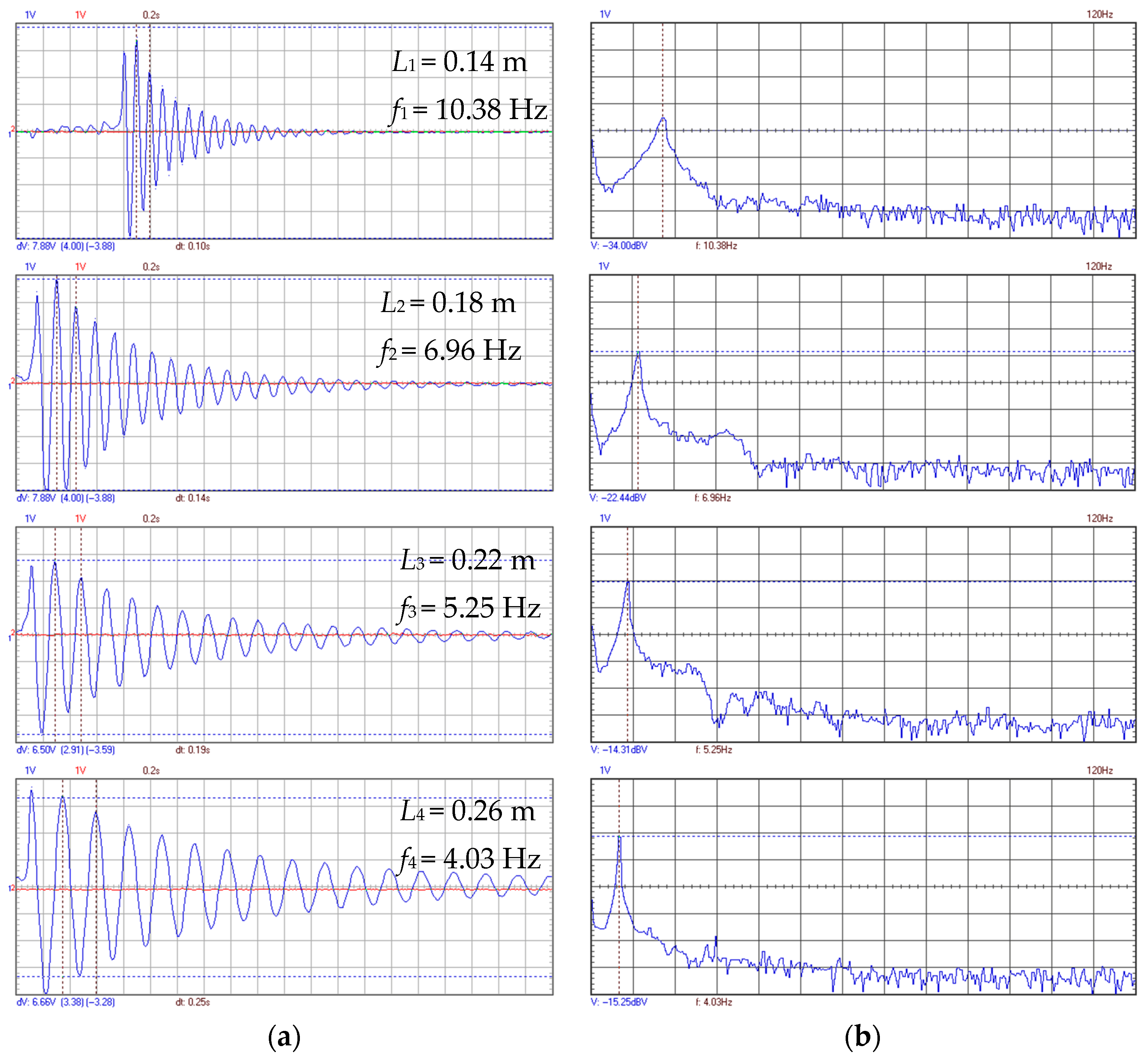
In Figure 3 are plotted the free vibration time records and their FFT spectra for cantilever length in the case of the cantilever beam reinforced with hemp fibers.
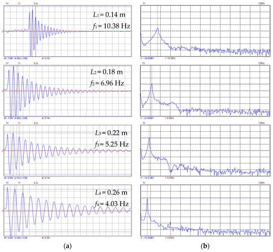
Figure 3.
(a) Free vibration time records for composite specimens with hemp fibers; (b) Amplitude spectra for composite specimens with hemp fibers.
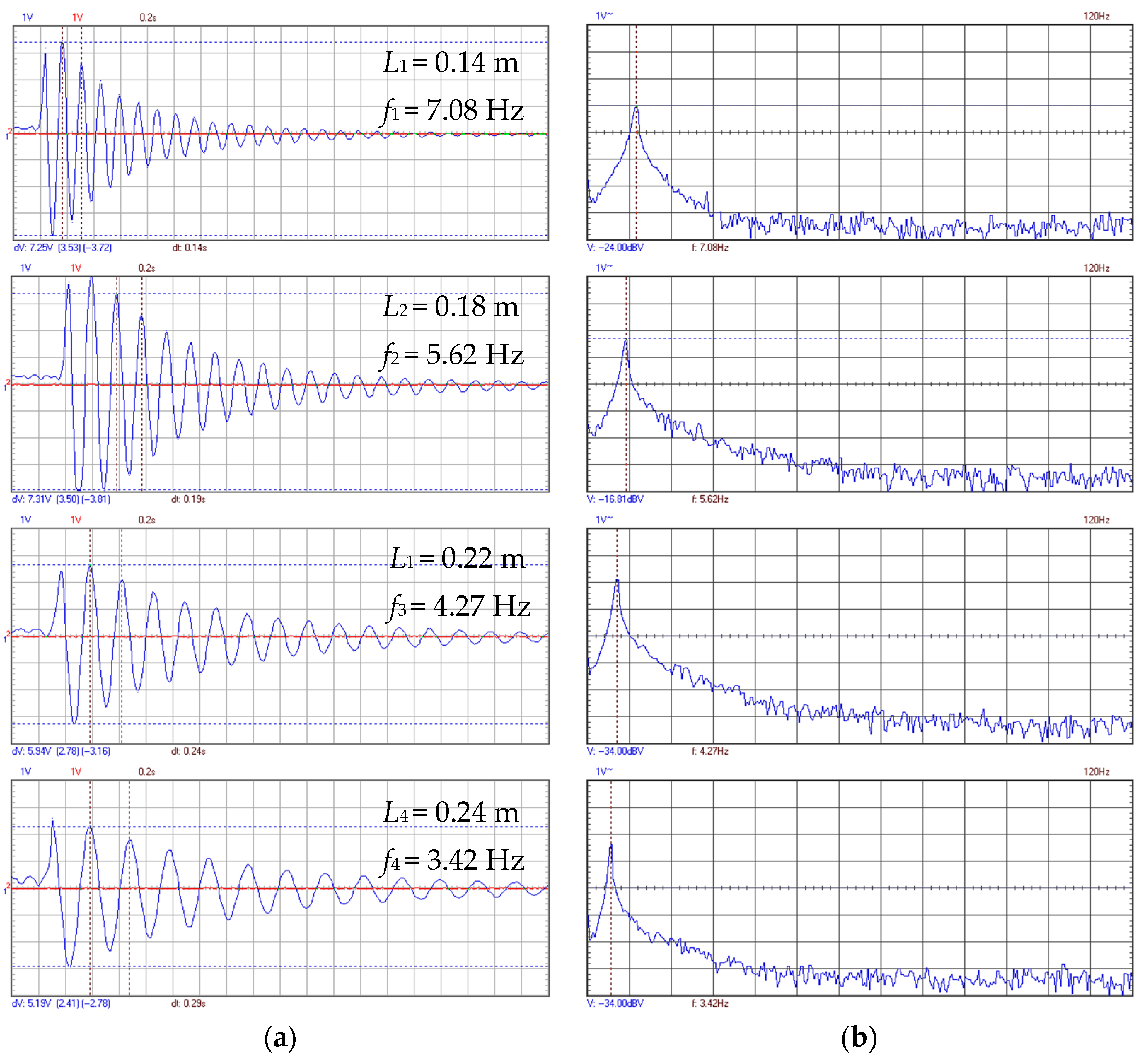
In Figure 4, the free vibration time records and the FFT spectra for the cantilever length are plotted, in the case of the specimens reinforced with coconut fibers.
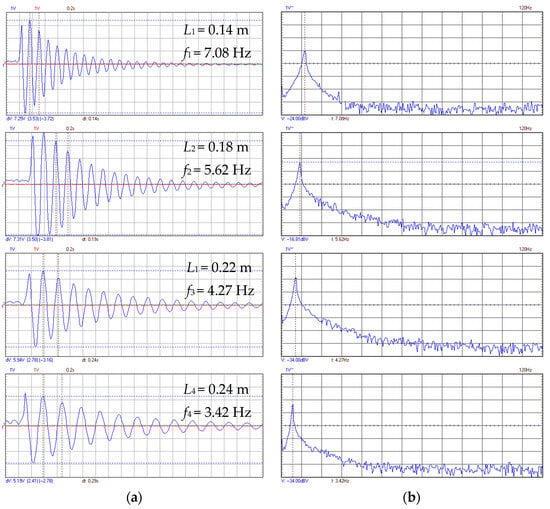
Figure 4.
(a) Free vibration time records for composite specimens with coconut fibers; (b) Amplitude spectra for composite specimens with coconut fibers.
In the case of the cantilever beam reinforced with hemp fibers, the following frequencies were obtained experimentally for the specified length: , , , and , and in the case of coconut fibers: , , , and .
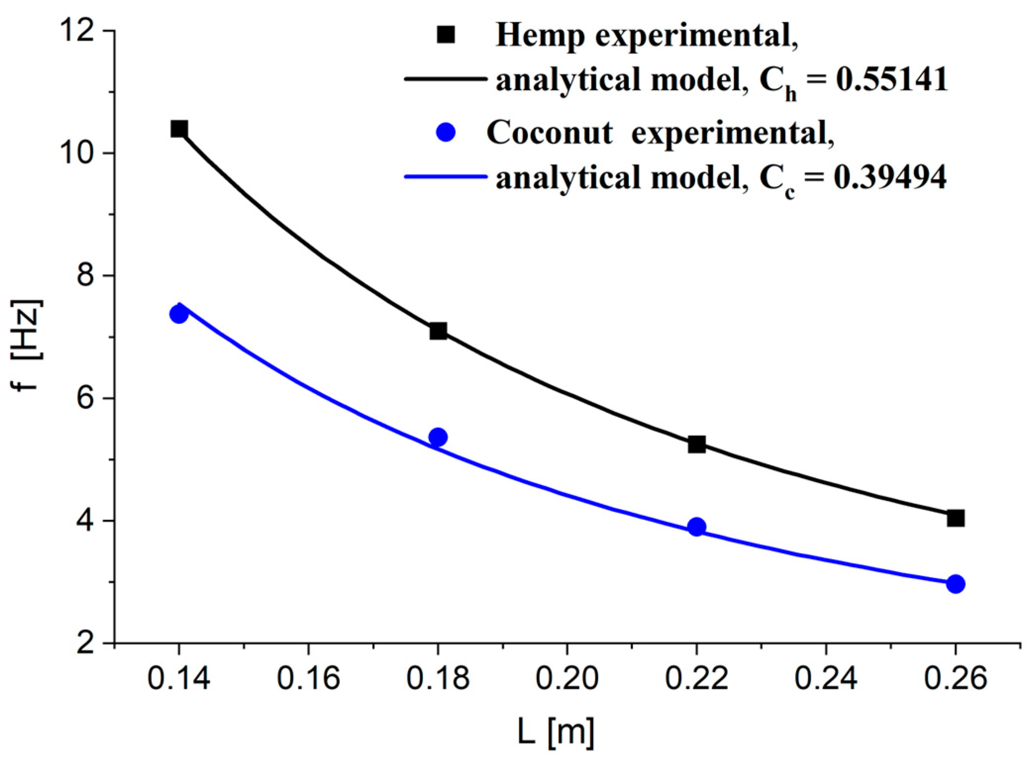
The results obtained by fitting the experimental data with analytical model are shown in Figure 5.
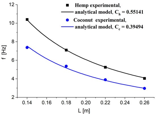
Figure 5.
Plots of experimental data and their fit by analytical model.
From relation (6), the value of the Young’s modulus for the composites with hemp fibers is and in the case of those with coconut fibers, .
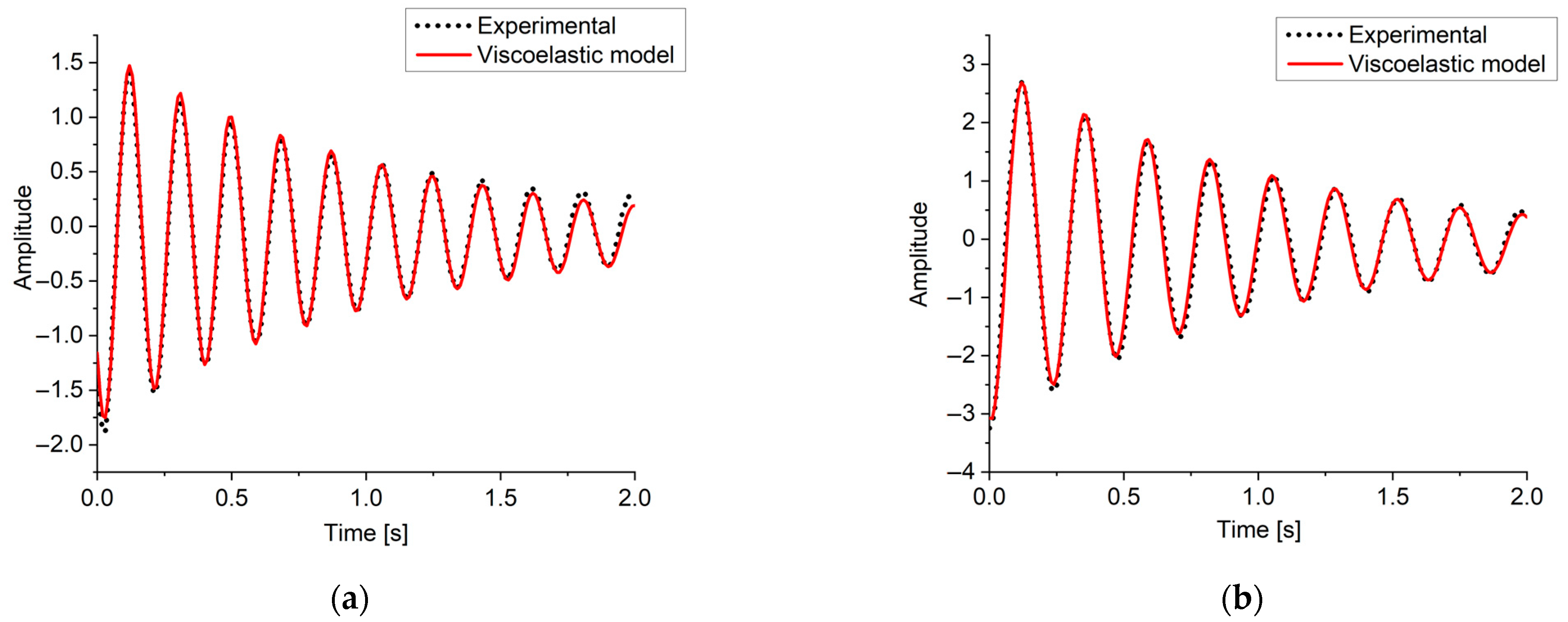
From the recorded free vibrations of the two types of material, shown in Figure 3a and Figure 4a, it can be observed that they exhibit viscoelastic behavior. This is highlighted by the fact that their time histories can be accurately described by the analytical solution of Equation (1), as illustrated comparatively for the samples with a length of 0.22 m in the following charts, in Figure 6.
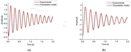
Figure 6.
Comparison of free vibration time records and analytical fit by viscoelastic model with (a) hemp fibers; (b) coconut fibers.
3.2. Numerical Results
In our case, when measurements are made for the first natural frequency, which corresponds to the natural bending mode, the acceleration transducer of mass was used, and the mathematical model is the one considered in Equation (17) representing mass-spring elements with a constant force , and m0 will be introduced as a concentrated mass at the top (free end) of the tested sample.
For numerical simulation, the same dimensions as for the experimental model were considered: , , , , , .
For the cantilever beam reinforced with hemp fibers for a cantilever beam density 900 kg/m3 and the Young’s modulus experimentally determined above , the values , , , and were obtained by numerical simulation.
In the case of the cantilever beam reinforced with coconut fibers for a cantilever beam with and density 750 kg/m3, , , , , , and , the values , , , and were obtained by FEM.
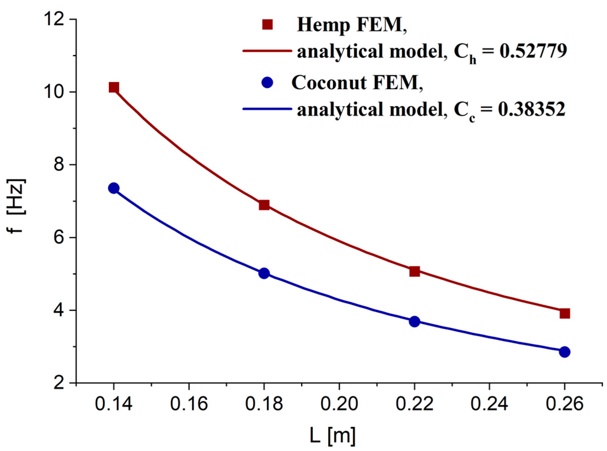
In Figure 7 are depicted the numerical results for the two considered composite beams with their fit using the analytical model .
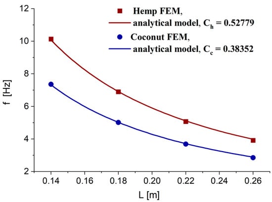
Figure 7.
Plots of numerical results (FEM) and their fit by analytical model.
For the composite beam made with hemp fibers, the value 0.52799 was obtained for the constant C, and for the cantilever beam reinforced with coconut fibers, the constant C had the value 0.38352.
Table 1 and Table 2 provide a summary of the experimental and numerical results obtained in the case of cantilever beams reinforced with hemp and coir fibers, respectively.

Table 1.
Compared results for hemp.
Table 2.
Compared results for coconut.
It can be observed that for the two considered composite beams, the damping ratio values are very small (0 < < 0.05) and, therefore, the damped and undamped natural frequencies of the system are very close.
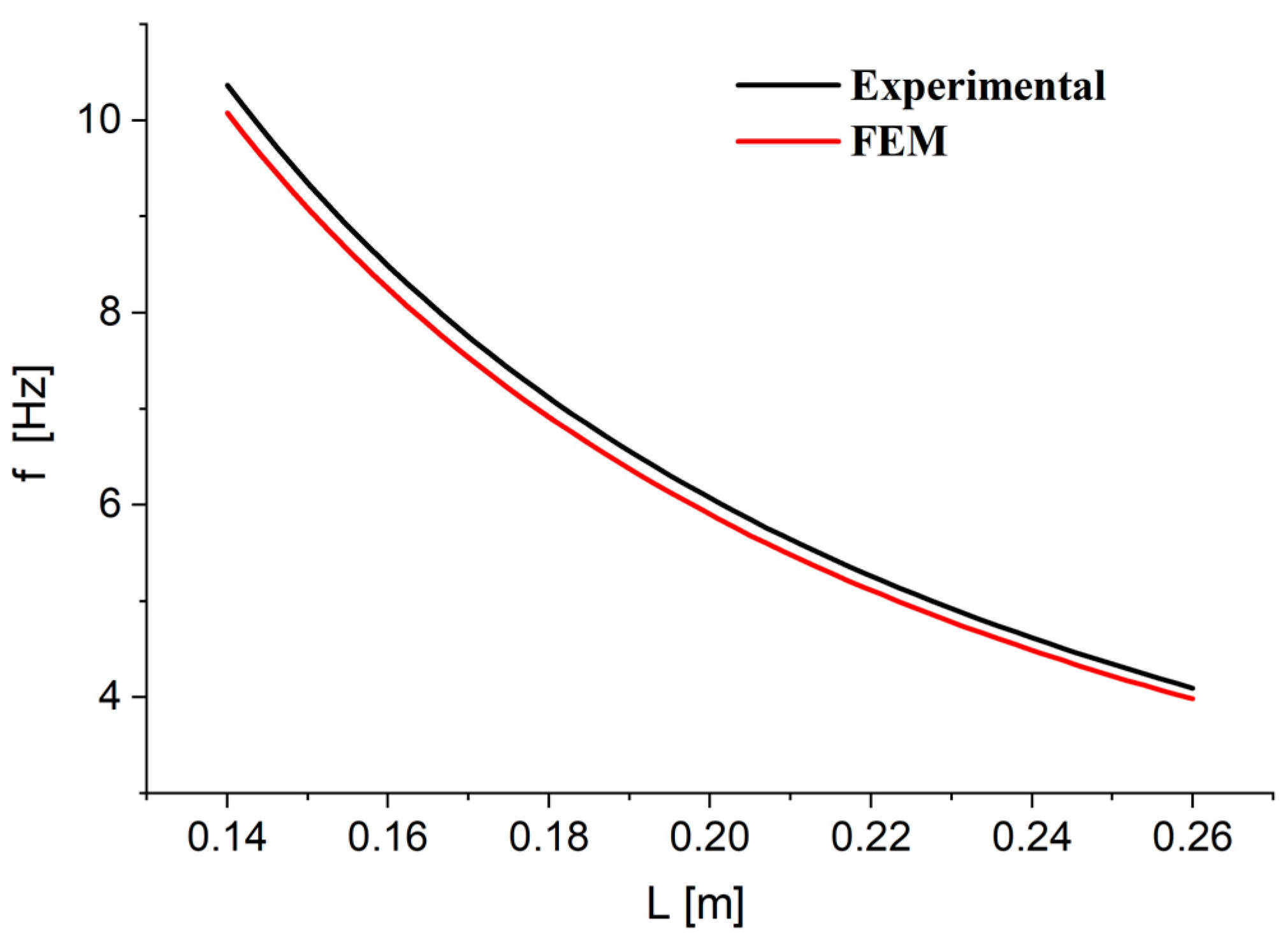
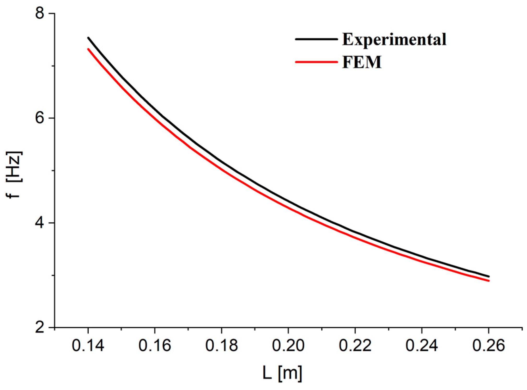
The comparison of experimental and numerical results in the case of the cantilever beam reinforced with hemp fibers is shown in Figure 8, and in the case of coconut fibers in Figure 9.
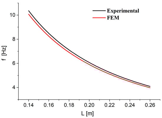
Figure 8.
Comparison of analytical model of experimental and FEM data in the case of hemp fibers.
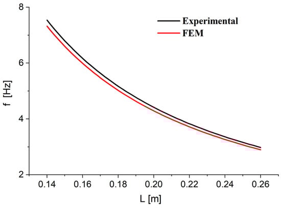
Figure 9.
Comparison of analytical model of experimental and FEM data in the case of coconut fibers.
The average relative error between the values obtained using the analytical model for the experimental and numerical data is 2.9% in the case of hemp fibers and 3% in the case of coconut fibers, consistent with the various specimen lengths. The differences between the values may come from slight dimensional and material variations, support and testing conditions, and instrument precision. The numerical uncertainty may arise from discretization errors, model assumptions, numerical approximations, and parameter uncertainties.
As one can observe, the comparison of numerical and experimental results validates the correctness and effectiveness of the proposed method.
4. Conclusions
The proposed non-destructive method presented in the current study represents an efficient method for assessing the Young’s modulus for composite materials reinforced with natural fibers. The technique consists in subjecting a set of composite samples taken from fabrication, in cantilever beam configuration, to an initial displacement. The same cantilever beam samples are tested at different lengths and their free vibration response and inherent dynamic characteristics are registered and determined (frequency and damping ratio). By identifying the longitudinal elastic modulus from the transverse vibration equation, which corresponds to the Euler–Bernoulli model of the beam embedded at one end, we create an inverse problem of the equilibrium equations of elasticity with an analytical method. Finally, with a numerical simulation method (FEM) and using the previously determined elastic constant, the experimental–analytical method is validated by obtaining the value of the first natural frequency with an acceptable error.
The errors induced by the inherent material inhomogeneity are averaged by fitting the experimental results to the analytical model of a cantilever lamellar spring with a mass attached at the free end. The advantage of this method is that it requires non-expensive laboratory equipment and can be used not only for rapid assessment of the value of Young’s modulus for different composite materials, but also for ensuring manufacturing constancy. The presented method can be further extended and validated experimentally for evaluating the shear modulus of composite materials reinforced with natural fibers.
Author Contributions
Conceptualization, T.S., A.-M.M. and N.P.; methodology, A.-M.M., T.S. and M.-R.A.; software, N.P. and C.-A.N.; validation, A.-M.M., T.S., N.P., C.-A.N. and M.-R.A.; investigation, M.-R.A., C.-A.N. and A.-M.M.; writing—original draft preparation, A.-M.M. and T.S.; writing—review and editing C.-A.N., A.-M.M. and N.P.; visualization, T.S. and N.P.; supervision, T.S. All authors have read and agreed to the published version of the manuscript.
Funding
This research received no external funding.
Institutional Review Board Statement
Not applicable.
Data Availability Statement
The data of this study are available from the corresponding authors upon reasonable request.
Acknowledgments
The authors gratefully acknowledge the support of the Romanian Academy.
Conflicts of Interest
The authors declare no conflict of interest.
References
- Liu, M.; Zhao, X. Overview of Non-destructive Testing of Composite Materials. In Proceedings of the 2020 3rd World Conference on Mechanical Engineering and Intelligent Manufacturing (WCMEIM), Shanghai, China, 4–6 December 2020; pp. 166–169. [Google Scholar]
- Qin, F.P.; Lu, F.C.; Huang, L. Numerical simulation and experimental validation of ratchetting deformation of short fiber-reinforced polymer composites. Compos. Part B-Eng. 2023, 266, 110974. [Google Scholar] [CrossRef]
- Cicco, D.D.; Taheri, F. Use of a Simple Non-Destructive Technique for Evaluation of the Elastic and Vibration Properties of Fiber-Reinforced and 3D Fiber-Metal Laminate Composites. Fibers 2018, 6, 14. [Google Scholar] [CrossRef]
- Neagoe, C.A.; Sireteanu, T.; Mitu, A.M. Characterization of anisotropic materials using a non-destructive free vibration method. Rom. J. Tech. Sci.-Appl. Mech. 2021, 66, 5–17. [Google Scholar]
- Wang, B.; Zhong, S.; Lee, T.-L.; Fancey, K.S.; Mi, J. Non-destructive testing and evaluation of composite materials/structures: A state-of-the-art review. Adv. Mech. Eng. 2020, 12, 1–28. [Google Scholar] [CrossRef]
- Meola, C. Nondestructive Testing in Composite Materials. Appl. Sci. 2020, 10, 5123. [Google Scholar] [CrossRef]
- Mitu, A.M.; Sireteanu, T.; Pop, N.; Chis, L.C.; Maxim, V.M.; Apsan, M.R. Numerical and Experimental Study of the Fatigue Behavior for a Medical Rehabilitation Exoskeleton Device Using the Resonance Method. Materials 2023, 16, 1316. [Google Scholar] [CrossRef]
- Mitu, A.M.; Sireteanu, T.; Meglea, C. Analytical and experimental assessment of degrading structures dynamic behavior. Rom. J. Acoust. Vib. 2012, 9, 3–8. [Google Scholar]
- Nguyen, D.H.; Ho, L.V.; Bui-Tien, T.; De Roeck, G.; Wahab, M.A. Damage evaluation of free-free beam based on vibration testing. Appl. Mech. 2020, 142–152. [Google Scholar] [CrossRef]
- Imran, M.; Khan, R.; Badsha, S. Vibration analysis of cracked composite laminated plate and beam structures. Rom. J. Acoust. Vib. 2018, 15, 3–13. [Google Scholar]
- Xiao, F.; Mao, Y.; Tian, G.; Chen, G.S. Partial-Model-Based Damage Identification of Long-Span Steel Truss Bridge Based on Stiffness Separation Method. Struct. Control Health Monit. 2024, 2024, 5530300. [Google Scholar] [CrossRef]
- Xiao, F.; Mao, Y.; Sun, H.; Chen, G.S.; Tian, G. Stiffness Separation Method for Reducing Calculation Time of Truss Structure Damage Identification. Struct. Control Health Monit. 2024, 2024, 5171542. [Google Scholar] [CrossRef]
- Xiao, F.; Yan, Y.; Meng, X.; Xu, L.; Chen, G.S. Parameter identification of beam bridges based on stiffness separation method. Structures 2024, 67, 107001. [Google Scholar] [CrossRef]
- Gu, X.; Hu, Q.; Mwamba, B.; Wang, Z.; Qi, L.; Wang, J.; Song, L.; Wu, J. Flexural Vibration Test Method for Determining the Dynamic Elastic Modulus of Full-Size Strawboards for Use in Transportation Framed Cases. BioResourses 2024, 19, 3149–3163. [Google Scholar] [CrossRef]
- Hui, L.; Peng, C.X.; Wanchong, R.; Xiao, P.L.; Bang, C.W. Identification of mechanical parameters of fiber reinforced composites by frequency response function approximation method. Sci. Prog. 2020, 103, 1–26. [Google Scholar]
- Gillich, G.R.; Praisach, Z.I.; Wahab, M.A.; Gillich, N.; Mituletu, I.C.; Nitescu, C. Free Vibration of a Perfectly Clamped-Free Beam with Stepwise Eccentric Distributed Masses. Shock Vib. 2016, 2086274. [Google Scholar] [CrossRef]
- Kubojima, Y.; Sonoda, S.; Kato, H. Practical techniques for the vibration method with additional mass: Effect of specimen moisture content. J. Wood Sci. 2017, 3, 568–574. [Google Scholar] [CrossRef]
- Itu, C.; Scutaru, M.L.; Vlase, S. The Quick Determination of a Fibrous Composite’s Axial Young’s Modulus via the FEM. Appl. Sci. 2024, 14, 6630. [Google Scholar] [CrossRef]
- Itu, C.; Scutaru, M.L.; Vlase, S. Elastic Constants of Polymeric Fiber Composite Estimation Using Finite Element Method. Polymers 2024, 16, 354. [Google Scholar] [CrossRef] [PubMed]
- Huang, Z.-M.; Zhang, C.-C.; De Xue, Y. Stiffness prediction of short fiber reinforced composites. Int. J. Mech. Sci. 2019, 161–162, 105068. [Google Scholar] [CrossRef]
- Huang, Z.-M. Constitutive Relation, Deformation, Failure and Strength of Composites, Reinforced with Continuous/Short Fibers or Particles. Compos. Struct. 2021, 262, 113279. [Google Scholar] [CrossRef]
- Katouzian, M.; Vlase, S.; Marin, M. Elastic moduli for a rectangular fibers array arrangement in a two phases composite. J. Comput. Appl. Mech. 2024, 55, 538–551. [Google Scholar]
- Lourenço, A.L.; Jager, N.; Prochnow, C.; Milbrandt Dutra, D.A.; Kleverlaan, C.J. Young’s modulus and Poisson ratio of composite materials: Influence of wet and dry storage. Dent. Mater. J. 2020, 39, 657–663. [Google Scholar] [CrossRef]
- Rangapuram, M.; Dasari, S.K.; Abutunis, A.; Chandrashekhara, K.; Lua, J.; Li, R. Experimental and numerical investigation of heat evolution inside the autoclave for composite manufacturing. Compos. Adv. Mater. 2024, 33, 1–19. [Google Scholar] [CrossRef]
- Singleton, T.; Saeed, A.; Strawbridge, L.; Khan, Z. Finite Element Analysis of Manufacturing Deformation in Polymer Matrix Composites. Materials 2024, 17, 2228. [Google Scholar] [CrossRef]
- Kurnatowski, B.; Matzenmiller, A. Finite element analysis of viscoelastic composite structures based on a micromechanical material model. Comput. Mater. Sci. 2008, 43, 957–973. [Google Scholar] [CrossRef]
- Lanzi, A.; Luco, J.E. Optimal Caughey series representation of classical damping matrices. Soil Dyn. Earthq. Eng. 2017, 92, 253–265. [Google Scholar]

Disclaimer/Publisher’s Note: The statements, opinions and data contained in all publications are solely those of the individual author(s) and contributor(s) and not of MDPI and/or the editor(s). MDPI and/or the editor(s) disclaim responsibility for any injury to people or property resulting from any ideas, methods, instructions or products referred to in the content. |
© 2024 by the authors. Licensee MDPI, Basel, Switzerland. This article is an open access article distributed under the terms and conditions of the Creative Commons Attribution (CC BY) license (https://creativecommons.org/licenses/by/4.0/).