Abstract
This article explores the practical implementation of autoencoders for anomaly detection, emphasizing their latent space manipulation and applicability across various domains. This study highlights the impact of optimizing parameter configurations, lightweight architectures, and training methodologies to enhance anomaly detection performance. A comparative analysis of autoencoders, Variational Autoencoders, and their modified counterparts was conducted within a tailored experimental environment designed to simulate real-world scenarios. The results demonstrate that these models, when fine-tuned, achieve significant improvements in detection accuracy, specificity, and sensitivity while maintaining computational efficiency. The findings underscore the importance of lightweight, practical models and the integration of streamlined training processes in developing effective anomaly detection systems. This study provides valuable insights into advancing machine learning methods for real-world applications and sets the stage for further refinement of autoencoder-based approaches.
1. Introduction
Anomalies, also known as outliers, rare occurrences, or deviations, represent data points or patterns that deviate from what is typically considered normal behavior. The anomaly detection process focuses on identifying data patterns that diverge from the anticipated norms based on prior observations. The capacity to pinpoint or recognize atypical behaviors can offer valuable insights across numerous sectors. By highlighting unusual instances or implementing a strategic response, an organization can conserve resources, reduce expenses, and retain clientele. Consequently, anomaly detection is widespread across various domains, such as IT analysis, detection of network breaches, medical analysis, prevention of financial fraud, assurance of manufacturing quality, and marketing and monitoring of social media activities.
Each application domain presents unique characteristics and challenges that drive specific requirements for anomaly detection systems. For example, in the financial sector, the large volume of transaction data combined with the high stakes of risk management necessitates anomaly detection systems that exhibit an exceptionally low false alarm rate. False positives in this domain can lead to unnecessary interventions, market volatility, and significant economic repercussions [1,2,3,4]. In healthcare, anomaly detection in medical imaging or patient monitoring demands high sensitivity, as undetected anomalies can result in misdiagnoses or delayed treatments, potentially jeopardizing patient safety [5,6,7,8,9]. Similarly, in manufacturing, ensuring product quality involves detecting subtle anomalies in sensor readings or production line data, requiring systems that can operate in real time and minimize downtime [10,11,12,13].
The network security domain often involves evolving threats and high-dimensional data, where adaptability to new patterns and low latency in detection are critical. Conversely, in marketing and social media analytics, the goal is to identify behavioral anomalies among users or trends, where the system must balance precision with the capacity to analyze large-scale data [14,15,16,17]. These diverse demands highlight the importance of tailoring anomaly detection systems to the specific requirements of each domain, which often influences the choice of models, training strategies, and evaluation metrics.
Despite the significant advancements in anomaly detection, current methods face challenges in achieving robust performance in complex, multi-dimensional data environments. Anomalies are often rare and context-dependent, making them difficult to identify using traditional approaches. Deep learning-based methods, such as autoencoders, have emerged as powerful tools for addressing these challenges. These methods excel in modeling non-linear dependencies and handling high-dimensional data, enabling them to detect subtle deviations from normal behavior.
Approaches based on deep learning, when applied to detect anomalies, offer several advantages. Firstly, those approaches are designed to work with multi-dimensional data. This facilitates the integration of information from many sources and eliminates challenges associated with individual modeling of anomalies for each variable and with aggregation of results. The deep learning approaches are also well-adapted to joint modeling of interactions between multiple variables concerning a given task; moreover, the deep learning models require minimal tuning to achieve good results and enable the determination of general hyperparameters (the number of layers, units per layer, etc.).
Another advantage is their efficiency. The deep learning methods offer the ability to model complex, non-linear dependencies within the data and use them to detect anomalies. The efficiency of the deep learning models may also scale with the availability of proper training data, making them appropriate for problems rich in data. Deep learning models can adapt to evolving network threats, particularly those trained semi-supervised [1]. They can detect anomalies based on learned patterns and deviations, even when the exact nature of the threat is new or unknown.
The use of mechanisms based on machine learning [18] (ML) and deep learning (DL) are efficient solutions that allow the detection of cyberattacks after the application of classic solutions such as the Intrusion Detection System (IDS), e.g., Snort, Suricata, or the Security Information and Event Management (SIEM) systems. Additional detection solutions based on ML/DL supplement the classic mechanisms that allow the detection of unknown and unauthorized operations in cyberspace. They may enable additional advanced safety data analysis, thus allowing us to find non-obvious connections. It is possible to discover valuable relation patterns between, e.g., adversaries and attacks, which are originally undetectable in the dataset acquired from the IT system [19,20].
This study addresses the challenges of anomaly detection by focusing on the potential of autoencoders and their enhancements to improve detection performance. While autoencoders have shown promise, there remains a need for a thorough evaluation of how architectural adjustments, training strategies, and loss functions affect their ability to detect anomalies in complex data environments.
The motivation behind this work stems from the need to enhance anomaly detection systems by systematically evaluating the performance of neural network models in a practical, network-focused context. While prior research has introduced numerous variations of different architectures, their direct application and comparison in the context of network anomaly detection require further exploration.
We systematically compare multiple autoencoder architectures across various parameter settings, including standard and Variational Autoencoders. This analysis highlights their strengths, limitations, and suitability for network anomaly detection.
We design and implement a robust, scalable experimental environment to evaluate autoencoders as anomaly detectors. This framework supports real-time network monitoring and integrates seamlessly with Big Data processing pipelines.
By focusing on the practical application and comparison of autoencoder-based models, this study advances the understanding of how deep learning can be effectively leveraged for anomaly detection in complex environments. The insights gained from our work contribute to developing more robust, efficient, and scalable solutions for network security.
2. Related Deep Learning Algorithms
This chapter contains an overview of significant architectures, the deep learning models, and the methods of their application in detecting anomalies. Detection of anomalies consists of learning the model of recognition of normal activities and then generating the results of anomalies that may be used to identify abnormal activities. Assuming that the majority of data points in an unflagged set is normal, it is possible to train a solid model in such an unmarked dataset and assess its efficiency (and tune the parameters of the model) using a small amount of unflagged data [21]. This hybrid approach is well-suited to network attacks, where numerous examples of a normal class and several known attacks may exist. However, in time, new types of classes may emerge. Moreover, the anomaly’s scale may change with other external factors. Such situations may require specification of the classes of the anomalies for which there are only a few or no flagged data. Therefore, a perfect solution is a semi-supervised classification, which allows the detection of known anomalies and anomalies that have not been seen so far.
The deep learning approaches discussed in the further part of the chapter belong to the encoder–decoder family: an encoder that learns to generate an internal representation of input data and a decoder that attempts to reconstruct original input data based on this internal representation. While precise coding and decoding techniques differ depending on the model, the general advantage they offer is the ability to learn the normal distribution of input data and appropriately construct the measure of the anomaly.
2.1. Autoencoders—AE
Autoencoders [22] are neural networks designed to learn low-dimensional representation, taking into account specific input data. They consist of two components: an encoder that maps input data into a low-dimensional representation (“bottleneck”) and a decoder that learns to map this low-dimensional representation back into the original input data. Thanks to this structure of learning, the encoder network learns a practical “compression” function that maps input data into a relevant low-dimensional representation to allow the decoder to reconstruct the original input data successfully. The model is trained via minimization of the reconstruction error, a difference (mean squared error) between the original input and the reconstructed output created by the decoder. In practice, the autoencoders were applied as a technique to reduce dimensionality. However, they are also used to remove noise from images, such as color images, ensure unattended extraction of features, and compress data.
It should be noted that the mapping function learned by the autoencoder is adapted to the distribution of training data. This means the autoencoder cannot reconstruct data that are significantly different from the data used during training. The properties of learning mapping specific to the distribution are beneficial for detecting anomalies.
The autoencoder detects anomalies by modeling normal behavior and then generating the anomaly result for each new data sample. To model normal behavior, one may adopt a semi-supervised approach, which assumes the training of the autoencoder using samples of standard data. As a result, the model learns the mapping function, which efficiently reconstructs normal data samples with a very minor reconstruction error. This approach is replicated during the test, where the reconstruction error is minor for normal data samples and significant for samples of abnormal data. To identify anomalies, one may use the result of the reconstruction error as a result of the anomaly and flag the samples with the reconstruction errors exceeding a given threshold.
2.2. Variational Autoencoders—VAE
Variational Autoencoder [23] (VAE) is an extension of an autoencoder. Just like an autoencoder, it contains encoder and decoder network components, but there are significant differences in its problem-learning structure. Contrary to the learning of mapping based on input data to a constant bottleneck vector (point estimation), VAE learns to map from input data to the distribution and reconstruct original data via sampling from this distribution using a hidden code.
The encoder network learns the distribution parameters (of a medium distribution and a variation of the distribution), which introduces a hidden code vector considering the input data. In other words, it is possible to draw samples of the bottleneck vector that “correspond” to the samples from the input data. The nature of this distribution may differ depending on the nature of the data. On the other hand, the decoder learns the distribution that introduces the original input data point, considering the hidden code samples (probability). Usually, this reconstruction space is modeled using an isotropic Gaussian distribution.
The VAE model is trained by minimization of the difference between the estimated distribution produced by the model and the actual data distribution. This difference is estimated using the Kullback–Leibler divergence, which determines the distance between two distributions by measuring the amount of lost information when a single distribution represents the other. Similarly to autoencoders, the VAE is applied in such cases as an unattended extraction of characteristics, reduction in dimensions, coloring of images, de-noising of images, etc. Moreover, considering that they use one distribution model, they may be used to generate samples in a controlled manner.
The probabilistic components introduced in VAE provide several advantages. First and foremost, VAE enables Bayesian inference; essentially, it is now possible to sample from a learned distribution of the encoder and decode samples that do not explicitly exist in the original dataset but belong to the same data distribution. Secondly, VAE learns a disjoint representation of the data distribution, i.e., a single unit in a hidden code is susceptible to only one generative factor. This enables specific interpretation of output data from VAE since we can change units in the hidden code to allow the controlled generation of samples. Thirdly, VAE ensures accurate probability measures, which offer a fundamental approach to quantifying uncertainty, such as the one used in practice.
Just like in the case of an autoencoder, one should start by training a VAE on samples of normal data. During the test, the anomaly result may be calculated using two methods. Firstly, it is possible to draw a hidden code sample from the encoder, considering input data and a sample of values reconstructed using the hidden code from the decoder, and then calculate the mean reconstruction error. Anomalies are flagged based on a certain threshold of the reconstruction error.
An alternative method is to derive an average and a variation parameter from the decoder and calculate the probability of a new data point belonging to the normal distribution on which the model is trained. If the data point lies in a region of low density (below a certain threshold), it will be flagged as an anomaly.
VAEs demonstrate a robust capability to generalize to unseen data by modeling normal network behavior and identifying anomalies, proving effective even when specific anomalies were not part of the training dataset.
2.3. Different Methods
In addition to the challenges neural networks face in anomaly detection, it is essential to recognize the existence of alternative methods for detecting anomalies, such as Generative Adversarial Networks (GANs), sequence-to-sequence (seq2seq) models, or Transformers [24]. These methods offer unique approaches but come with their own set of considerations and potential drawbacks.
Generative Adversarial Networks [25] (GANs) are neural networks designed to learn a generative model of input data distribution. In a traditional model, they are composed of a pair of neural networks known as the G generator and the D discriminator. Both networks are trained together and play a competitive “game” to learn the distribution of the X input data.
The G generator network learns to map from a random noise of constant dimension (Z) to X samples, which strictly resemble elements of input data distribution. The D discriminator learns to correctly differentiate true samples from source data (X) from false samples (X*), which G generates. In each era during training, the G parameters are updated to maximize their capability to generate samples that are impossible to differentiate by D. In contrast, the D parameters are updated to maximize the decoder capability to differentiate true X samples from generated X samples correctly. As the training progresses, G becomes proficient in producing samples similar to X, and D also improves its ability to differentiate true samples from false ones.
However, classic GANs do not have a direct mechanism that would allow generating a sample similar to a known sample; therefore, it is impossible to use them in the analysis process to detect hidden contents. This problem can be combated by using modifications of those networks. One such modification is BiGAN [26]. In simple terms, its structure includes a third model, i.e., an encoder that learns from the reversed mapping of the generator; the encoder learns to generate a constant Z vector based on the sample. Due to this change, the input to the discriminator is also modified; the discriminator now adopts pairs of input data that include a hidden representation (Z and Z*) and the data samples (X and X*). Then, the E encoder is trained with the G generator; the G learns the distribution that derives the X samples, considering the hidden Z code, while the E learns the distribution that derives Z based on the X sample.
Mappings learned by the GAN components are specific to the data used in the training. For example, the generator component in a GAN trained using cat images will always generate an image that looks like a cat, considering any hidden code. During the test, one may use this property to conclude how much a given input sample differs from the data distribution based on which the model was trained.
Sequential models are a class of neural networks designed mainly to learn mappings between data that are best represented as sequences (an analysis of subsequent packets is one of the best cases of their use). Sequential models are usually composed of an E encoder, which generates a hidden representation of input data, and a D decoder, which adopts the representation of the encoder and sequentially generates a set of output data. Traditionally, the encoder and decoder are composed of long short-term memory [27] (LSTM), which is appropriate for modeling time relations within transformed input data.
The LSTMs are perfect for modeling data with time dependencies but may be slow during evaluation. Each single token, a sample at the model’s output, is generated sequentially in each time step, where the total number of steps is the length of the (appropriately transformed) input vector.
It is possible to use the encoder–decoder structure to detect anomalies by changing the sequential model to make it work like an autoencoder, thus training the model to derive the same tokens as input data but shifted by 1. This way, the encoder learns to generate a hidden representation, allowing the decoder to reconstruct input data similar to the examples visible in the training dataset.
A newer solution for problems associated with the LSTM model is networks containing the attention mechanism [24]. They allow sequential data in parallel, considering adjacent samples, thus eliminating the problem of sequential generation.
One may apply a semi-supervised approach to identify anomalies, in which the sequence model is trained using normal data. During the test, it is possible to compare the difference (mean squared error) between the output sequence generated by the model and its input data. Just like in the case of the previously discussed approaches, this value will assess the level of occurrence of anomalies.
A significant development in deep learning is represented by transformers and attention mechanisms [24,28], which provide special powers for simulating intricate relationships in data. Transformers use self-attention mechanisms, which assess each data point’s significance about the others in a sequence, in contrast to conventional sequential models like RNNs or LSTMs. This makes it possible for transformers to efficiently capture global context, which is essential for anomaly identification where connections between far-flung features may be necessary. This method is further enhanced by positional encoding, which ensures the model can handle non-sequential input without losing structural or temporal linkages by embedding information about the order of data points.
Transformers excel in anomaly identification by modeling long-range dependencies and complex interactions between input features. This broad context awareness allows them to detect tiny, context-dependent anomalies in datasets like network traffic. Transformers’ parallelized data processing capabilities enable them to handle large-scale, high-dimensional datasets more efficiently than traditional sequential models, resulting in significant computational savings.
Another significant advantage of transformers is their versatility. Integrating transformers with existing architectures, such as autoencoders or generative models, enhances latent representations used for anomaly identification. This combination can yield expressive and context-aware features, producing more precise and robust detection capabilities. Transformers have been used in various anomaly detection activities, such as network traffic analysis, where they scan packet sequences to discover odd patterns, and industrial systems, where they examine telemetry data to detect early indicators of equipment breakdown.
While transformers have particular advantages, their reliance on massive datasets and significant computational resources creates issues. To improve performance for specific anomaly detection applications, hyperparameters such as the number of attention heads and layers must be carefully tuned. Despite these limitations, transformers have demonstrated considerable potential when comprehending long-term dependencies and relationships in high-dimensional data.
2.4. Summary
Considering the differences between the deep learning methods discussed above, selecting the appropriate model may be difficult. Table 1 shows the comparison of the described DL methods.

Table 1.
Comparison of DL methods.
When data appear sequentially during network issues and hidden channels, the seq-to-seq model may model those dependencies, thus providing better results. However, why not use a “window” data analysis or limit its use to single samples? However, keep in mind that deep neural networks use their full potential when they are used for multi-dimensional data; hence, about the speed of operation, the necessity to have a large set of data and potential difficulties in the learning process (e.g., GAN mode collapse) in case of simple, linear applications, classic methods may be a better solution. In different network traffic scenarios, the choice of method depends on the specific requirements. AE and VAE are suitable for scenarios where the modeling of normal behavior and detection of deviations are critical [20].
Applying GANs, seq2seq, transformers, and similar complex models to anomaly detection should be carefully considered. These methods can sometimes represent an over-complication, where the model’s sophistication does not necessarily translate to better performance in practical anomaly detection tasks. The complexity of these models can lead to increased computational requirements and slower operational speeds, which the incremental gains in accuracy or detection capabilities may not justify. Therefore, these advanced methods should be case-specific and thoroughly evaluated against the nature of the data and the specific requirements of the anomaly detection task.
Despite the apparent advantages of deep learning models in anomaly detection, their implementation is not without challenges.
Data Imbalance: Typically, datasets contain a vast majority of “normal” data points compared to a relatively small number of anomalies. This imbalance makes it difficult for the neural network to learn the characteristics of anomalies effectively, as the overwhelming presence of normal data can lead to a bias toward classifying most inputs as normal.
Defining the Hidden Space Representation: The effectiveness of an autoencoder in anomaly detection hinges on its ability to learn a comprehensive representation of the data in its hidden space. The challenge lies in designing an autoencoder that can capture the essence of normal data so that anomalies are distinguishable when they fail to conform to this learned representation. This requires a careful balance between making the hidden space too general, which might overlook subtle anomalies, and making it too specific, which could falsely flag normal variations as anomalies.
Selection of Loss Functions and Thresholds: The choice of loss function can significantly impact anomaly detection performance. The loss function must be sensitive enough to highlight deviations in the reconstruction of data points yet robust enough to ignore insignificant variations. Additionally, setting the appropriate threshold for distinguishing between normal and anomalous data is crucial and challenging, as it often requires domain knowledge and iterative experimentation.
Complexity of Anomalies: Anomalies can manifest in various forms and might not always be straightforward deviations from the norm. Some anomalies could be contextual, where their anomalous nature is only apparent in certain situations or combinations of features. This complexity necessitates a neural network architecture that can understand and model the intricacies of normal behavior and its exceptions.
Evolving Data Patterns: In many applications, the definition of normal behavior can change over time. This evolution poses a challenge for anomaly detection systems, which must adapt to new patterns of normal behavior without losing the ability to detect true anomalies.
The detection difficulty of network anomalies lies in the subtlety and diversity of such irregularities, which often blend in with standard traffic patterns, making them hard to identify without sophisticated analysis. Furthermore, for example, the dynamic nature of network traffic, combined with the continuous evolution of cyber threats, adds to the complexity of establishing a reliable detection system. Moreover, the high dimensionality of data and the need for real-time detection introduce additional computational burdens. These challenges underscore the need for ongoing research and innovation to refine deep learning methods for more accurate and efficient anomaly detection.
3. Internal Analysis of the Impact of the Autoencoder Network Structure and Training Method on Anomaly Detection
For analysis and description of practical usage, this article introduces a deep learning (DL) framework for detecting network traffic anomalies. Our research presents a DL-based solution that addresses the inherent limitations of traditional anomaly detection systems. By innovatively integrating multi-dimensional data, our approach simplifies the complexities associated with individual anomaly modeling and enhances the aggregation process of anomaly detection results.
3.1. The Architecture of the Proposed Practical Usage
Apart from selecting appropriate machine learning and deep learning methods, an essential contribution of our work is ensuring the efficient operation of detection mechanisms in real-world production environments. We achieved this by designing an application capable of handling large datasets for prediction and learning nearly in real time. This efficiency is made possible through our unique implementation of techniques supporting high-intensity data streams, such as asynchronous communication, queuing, NoSQL databases, and a Big Data processing platform (Figure 1).
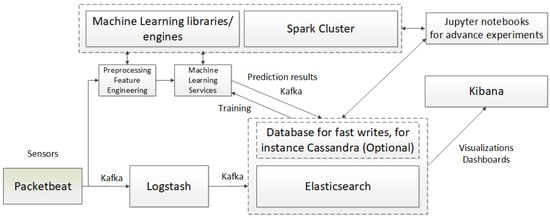
Figure 1.
General system architecture—illustrating the key components of the system, their interconnections, and the technologies used for implementation.
We assume that the network traffic data are downloaded using a probe; such a sensor may, e.g., use the Packetbeat mechanism. This network packet analyzer operates in real time to provide an application monitoring system. Packetbeat captures the network traffic between the application servers, ensures decoding of the protocols of the application layer (HTTP, MySQL, Redis, etc.), correlates requests with responses, and registers interesting fields for each connection. Packetbeat is integrated with the applied technological stack: Elasticsearch, Logstash, and Kibana (ELK) [29]. The sensor or a set of sensors is located in the critical places of the IT system topology, thus ensuring optimal network activity monitoring [30].
The network traffic data from the measuring probe are streamed to the Logstash mechanism and preprocessing, feature engineering, and machine learning services. Kafka is a distributed streaming system composed of servers and clients communicating with each other via a highly efficient TCP network protocol, thus allowing the comprehensive implementation of cases of high-intensity event streaming. Logstash is a protocol for processing data on the server’s side, which downloads data (network traffic data in this case), transforms it, and then sends and stores it in the NoSQL Elasticsearch base. Machine learning methods then use stored network traffic data; the system operator may also read them through dashboard-type panels in the Kibana service [30].
The network traffic characteristics are normalized and then additionally processed using the Apache Spark cluster and machine learning mechanisms (Big Data and Machine Learning Engine). This may consist of creating new characteristics derived from the original attributes of the input vector for the network traffic. Apache Spark is an open-source parallel processing platform that supports memory processing to improve the performance of applications that analyze Big Data. The Spark platform processes large amounts of data in memory significantly faster than alternatives based on hard drives [31]. A processed input vector is streamed to the machine learning service in which created models implement the prediction process, or a given data sample represents regular or unauthorized traffic. Vectors are stored in the Elasticsearch base together with the prediction results.
Elasticsearch is a distributed, free-of-charge, and open search engine that allows for the analysis of all types of data. Elasticsearch is a central component of the Elastic Stack—a set of tools for obtaining, enhancing, storing, analyzing, and visualizing data. After indexing datasets in Elasticsearch, users may launch submitted requests and use aggregation to download a comprehensive summary of their data. Elasticsearch, Logstash, and Kibana software are commonly referred to as the ELK stack. Kibana is a tool used to visualize and manage data for Elasticsearch by providing real-time histograms, line graphs, circle diagrams, and maps. Moreover, to improve the possibility of supporting the recording of a high-intensity data stream, one may use the NoSQL Cassandra base that cooperates with Elasticsearch.
The characteristics processing (Preprocessing Feature Engineering) and machine learning components [32] are implemented using the H2O Wave libraries [33]. This is an open-source environment written in Python. H2O Wave allows the creation of interactive AI applications in real-time, offering advanced visualizations of the user interface and charts, dashboard templates, dialogs, motifs, widgets, etc. For the needs of the implemented system, we created a dashboard to trigger the learning process and supervise the prediction process. The Big Data and Machine Learning Engine works as a Spark and H2O cluster, allowing the selected algorithms to operate in a standard mode. This ensures an excellent capability to support the data stream and improves scalability. Services in Wave establish communication with the cluster, and upon selecting messages for prediction, they send the messages to the cluster, obtain the result, and stream it to the Elasticsearch base.
In the presented system, the H2O platform was used as the ML engine; this in-memory machine-learning solution may be integrated with the Apache Spark cluster (Figure 2). Spark and machine learning services are active at each cluster node (Worker Node). The operation of those nodes is coordinated by the Driver Node, which supports the machine learning and Spark context. It should be noted that together with the development of the system, other libraries may be used for machine learning, e.g., Keras, PyTorch, etc.
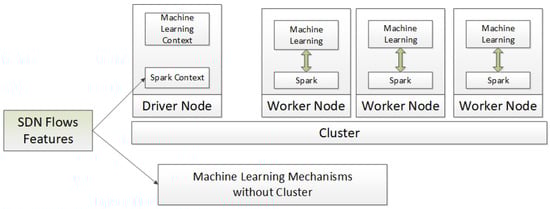
Figure 2.
The Big Data and Machine Learning Engine component architecture—technologies used for implementing the cluster-based variant.
Apart from predefined machine learning methods, the proposed solution allows the launch of the Jupyter Notebooks. Using Python, one may design new, more advanced experimental solutions for attack detection, aggregation, and analysis. For this purpose, it is possible to download data stored in Elasticsearch and use the Big Data and Machine Learning Engine components. Obtained results are presented as reports that are easy to interpret.
3.2. Description of Selected Machine Learning Methods
There are many different types of autoencoder architectures designed for network traffic analysis [34,35,36,37,38,39,40,41,42], and the performance of these models heavily depends on the type of data available. We introduced three distinct methods in developing our machine learning module, marking a significant contribution to network anomaly detection. This article aims to demonstrate that these architectures, whether performing better or worse, can be improved through iterative modifications introduced in the three methods discussed. Implementing three methods based on a structurally similar model allows for analyzing the impact of individual components in understanding complex structures such as neural networks. Two of these methods focus solely on analyzing normal data, while the third, an experimental approach, also incorporates abnormal data during training. Including abnormal data is a crucial innovation, allowing for a more comprehensive understanding and detection of network anomalies. The first method is an autoencoder, a model comprising three hidden encoder layers and three hidden decoder layers. Unique to our implementation, as depicted in Figure 3, is the careful tuning of the model’s architecture. The autoencoder was designed with specific input dimensions and varying hidden and latent dimensions, allowing us to thoroughly explore the impact of these parameters on the model’s performance. Our approach to training this model, based on minimizing the mean squared error, is tailored to suit the characteristics of network traffic data, ensuring high fidelity in anomaly detection.
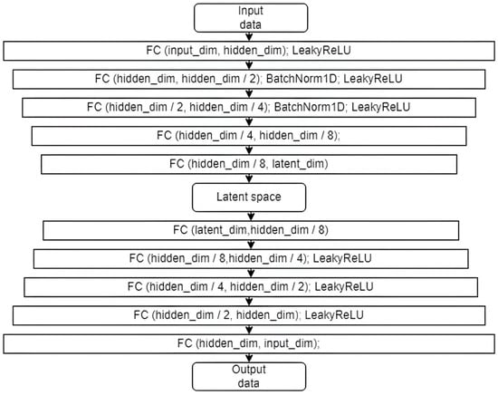
Figure 3.
Autoencoder model (FC—fully connected layer, input_dim—dimensionality of input data; hidden_dim—dimensionality of the hidden spaces that adopt the following values during the experiments: 64, 128, or 256; latent_dim—dimensionality of the “bottleneck” that adopts the following values: 8, 16, 32, 64, 128, or 256; output data—same dimensionality as input).
The training of the model was carried out based on the mean squared error:
where is the number of input data, is the characteristics of input data, and is the reconstructed characteristic of input data.
The second model tested in this article is the Variational Autoencoder. This model’s difference is that it projects a fully connected last layer into two hidden spaces representing the mean and the probability distribution variation. Similarly to the standard autoencoder, the Variational Autoencoder is an architecture that is composed of both an encoder and a decoder; this architecture is trained to minimize the reconstruction error between coded–encoded data and the initial data. However, the encoding–decoding process was modified to introduce a certain regularization of the hidden space. Instead of coding input data as a single point, they are encoded as a distribution in the hidden space. The model is then trained in the following manner: Input data are encoded as a distribution on the hidden space, a point from the hidden space is sampled from this distribution, then the sampled point is decoded, and the network retroactively propagates the calculated reconstruction error. In practice, the coded distributions are selected as normal, allowing the encoder to train it to return the mean and covariance matrix. The cost function, which is minimized during the training of the VAE, consists of the “cost of reconstruction” (on the final layer), the purpose of which is to make the encoding–decoding scheme as precise as possible, and the “regularization cost” (on the hidden layer), which aims to regularize the organization of the hidden space by bringing the distributions returned by the encoder closer to the standard normal distribution. This regularization term is a Kullback–Leibler divergence between the returned and standard Gaussian distributions. As a part of the experimental training of the model, the following so-called ELBO function is used:
In the conducted experiments, p is the normal probability distribution (0.1) that constitutes the target for the q probability distribution modeled based on input data.
To enable the use of the obtained data on anomalies in the experiments, a modified M-ELBO cost function [43] was also introduced:
where Wis the number of samples in the batch; if the introduced sample is an anomaly or if the introduced sample is normal; and . An assumption of such a cost function is x-to-z mapping, regardless of whether the sample is normal. However, the model is taught to reconstruct normal data only.
The modified M-ELBO cost function is tailored to handle normal and abnormal samples, a crucial enhancement for anomaly detection in network traffic. This cost function aims to allow for a more nuanced and compelling training process, distinguishing between normal and anomalous samples while primarily teaching the model to reconstruct normal data.
Our contribution to network anomaly detection by implementing these machine learning methods is comprehensive and nuanced. The core of our innovation lies in adapting existing models to meet the unique challenges presented by network anomaly detection. We have carefully selected and configured models such as the autoencoder and the Variational Autoencoder (VAE), fine-tuning their architectures to suit the intricacies of network traffic data. We compare the impact of the construction of various model components on the results and the adopted cost functions.
Through these methodological choices, we have significantly advanced the application of machine learning in network security. Our work demonstrates how existing tools and functions can be effectively leveraged and adapted to create innovative and highly effective solutions to the complex anomaly detection problem.
3.3. Description of Experiment
The publicly available InSDN test dataset was used to assess the efficiency of neural network methods [44]. The scientific environment positively assesses the dataset in question—it considers the types of current attacks generated using actual tools for penetration tests. It has characteristics based on flow-based features without the packet payload, e.g., the duration of the flows, the number of packets, and the number of bytes. The set includes labeled data with seven attack classes: DoS, DDoS, Probe, Web Attacks, R2L (Remote to Local), BFA (Brute Force Attack), and U2R (User to Root). It should be noted that giving a label to a teaching set is a technologically costly process and is hard to achieve in the actual environment in terms of the analysis of cyberattacks. In the case of machine learning, in the anomaly detection approach, one may treat the training data as a normal activity; however, an unauthorized action during the training processes cannot be ruled out. Authors extracted over 80 features categorized into eight groups:
Network Identifiers Attributes: These include basic information defining source and destination flow, such as IP addresses, port numbers, and protocol types.
Packet-Based Attributes: Information about packets, including total counts in both forward and backward directions.
Bytes-Based Attributes: Data on the total number of bytes in both forward and backward directions.
Interarrival Time Attributes: Details on the interarrival times in both directions.
Flow Timers Attributes: Information about the timing of each flow, including active and inactive periods.
Flag Attributes: Data on flags like SYN Flag, RST Flag, Push Flag, etc.
Flow Descriptors Attributes: Traffic flow information, including packet and byte counts in both directions.
Subflow Descriptors Attributes: Information regarding subflows, such as packet and byte counts in forwarding and backward directions.
The 80% set was used during our training, while the 20% set was used to carry out tests—as a result, a test set including 55,003 anomaly samples and 13,733 normal samples was obtained.
To ensure training stability, we applied standard preprocessing techniques:
Normalization: The features were normalized to values from 0 to 1. This step is essential for ensuring that the input features have a similar scale, which helps improve the performance and training stability of deep learning models. Mainly, the normalization process included max normalization based on the entire dataset’s specific columns.
One-Hot Encoding: This technique was used for categorical data transformation, a common preprocessing step in machine learning to handle non-numeric features effectively, like a flow type.
Removal of Insignificant Characteristics: Certain features deemed insignificant, such as ’FlowID’, were removed from the dataset. This step helps reduce the dimensionality and focus the model on more relevant features.
While the order in which data is entered during training can affect model learning in some instances, it was not explicitly considered in this study as the data were presented in a vectorized format. This preprocessing ensured uniformity across all samples, minimizing the potential impact of data order on training. To ensure further stability, we incorporated typical neural network stabilization techniques, including dropout regularization, batch normalization, and learning rate scheduler.
As a result, a 69-element vector was obtained at the input. The qualifying threshold was determined based on a test set for each model to select the most optimal one. Therefore, the experiments include testing the capabilities of the model to reconstruct and thus distribute the samples in the best manner possible. In the production environment, this threshold should be lowered due to the target maximization of the parameter (True Positive—correct detection of an anomaly; False Negative—wrong classification of an anomaly as a normal sample). Ultimately, values similar to the threshold should be collected for labeling and used to provide additional training for the model. For experimental purposes, the primary indication of the model’s efficiency was the classification’s precision. The Adam optimizer was used during the training process, and it did not stop until the accuracy of the test data decreased. Each model’s training was conducted six times for various initial learning rates (0.01, 0.001, and 0.0001) and batch sizes (32,128). In total, 324 experiments were conducted.
The training process of the deep learning models in the paper, focusing on hyperparameters, training duration, and steps taken to prevent overfitting, can be summarized as follows:
- Selection of Hyperparameters:
- Autoencoder (AE) and Variational Autoencoder (VAE): The selection of hyperparameters was crucial for both AE and VAE models. The hidden and latent dimensions were varied to understand their impact on model performance. Specifically, hidden dimensions were experimented with at 64, 128, or 256, and latent dimensions at 8, 16, 32, 64, 128, or 256. This variation allows for an exploration of how the complexity of the model affects its ability to reconstruct and detect anomalies.
- Cost Function Choices: The VAE model used a specialized cost function comprising reconstruction and regularization costs. This choice of cost function is essential as it balances the model’s ability to reconstruct input data while accurately maintaining a well-organized hidden space.
- Training Duration:
- Iterations Per Epoch: Each epoch of the training process consisted of approximately 2000 iterations. This indicates a comprehensive training procedure per epoch, allowing the models to learn sufficiently from the training data in each pass.
- Total Iterations: The training continued until there was no further improvement in the test set performance. This approach led to training durations that varied significantly, with some models reaching up to 200,000 iterations while others concluded around 20,000 iterations.
- Adaptive Training Duration: This adaptive approach to training duration, which continues until the test performance plateaus, effectively ensures that the models are neither under- nor over-trained. It allows each model to learn at its own pace based on the architecture’s complexity and the data’s nature.
- Preventing Overfitting:
- Dynamic Stopping Criterion: The decision to stop training when the test set performance on accuracy ceased to improve is an example of a dynamic stopping criterion, akin to early stopping. This method is crucial in preventing overfitting, as it ensures that the model does not continue to learn the idiosyncrasies of the training data that do not generalize to unseen data.
- Monitoring Test Performance: Regularly monitoring the model’s performance on the test set during training allows for a balanced approach, ensuring that the model is effectively learning the underlying patterns in the data without memorizing the training set.
- Regularization Techniques: Regularization in the cost function of the VAE is a direct method to prevent overfitting. The Kullback–Leibler divergence in the VAE’s cost function ensures that the model memorizes the training data and learns a more generalized representation.
- Hyperparameter Tuning: This study implicitly addressed overfitting by experimenting with different hyperparameters, particularly the size of the latent space in autoencoders. Smaller latent spaces can help prevent the model from capturing too much noise and overfitting.
- Dataset Splitting: Using an 80–20 split for training and testing ensures that the model’s performance is evaluated on unseen data, a standard practice for mitigating overfitting.
3.4. Results of Experiments
Our exhaustive analysis of different combinations of deep learning (DL) models and parameters has significantly contributed to understanding the application of reconstruction-based DL methods in anomaly detection. By exploring various configurations of autoencoders, Variational Autoencoders (VAEs), and Modified Loss Variational Autoencoders, we have provided valuable insights into the efficacy of these models in detecting network anomalies.
As summarized in Table 2, the results reveal that the VAE model with a modified cost function consistently outperforms the other models. This highlights the importance of incorporating anomalous data in training despite not directly reconstructing it. An interesting observation from our experiments is that while the autoencoder showed acceptable performance even with large latent dimensions, it was more prone to overfitting, underscoring the need for careful model configuration.
Table 2.
The efficiency results of models, including a reference to the best one. The bolded values indicate the best results for each model.
The paper’s approach to evaluating the deep learning models for anomaly detection focuses on three key performance metrics: accuracy, specificity, and sensitivity [45]. Let us discuss the relevance and importance of each of these metrics in the context of anomaly detection:
Accuracy:
- Measures the overall effectiveness of the model in classifying both normal and anomalous instances correctly.
- It is a primary indicator of model performance, providing a high-level view of how well the model performs across all classifications.
Specificity:
- Specificity measures the proportion of actual negatives (normal instances) that are correctly identified.
- High specificity in network anomaly detection indicates the model’s effectiveness in correctly identifying normal traffic, which is crucial to minimizing false alarms (false positives).
Sensitivity (also known as recall):
- Sensitivity assesses the model’s ability to correctly identify positives (anomalies).
- This metric is crucial in anomaly detection, as it reflects the model’s capacity to detect actual threats or anomalies in the network traffic.
The choice of these metrics is particularly apt for anomaly detection in network traffic scenarios. In such applications, it is critical not only to identify anomalies accurately (high accuracy) but also to ensure that everyday activities are not misclassified as anomalies (high specificity) and that actual anomalies are not missed (high sensitivity).
Accuracy provides a balanced view of overall model performance. At the same time, specificity and sensitivity offer insights into the model’s ability to handle the nuances of anomaly detection—distinguishing between normal operations and potential threats. This combination of metrics offers a comprehensive evaluation of the model’s performance, considering the critical aspects of anomaly detection where false positives and false negatives have significant implications.
The statistical analysis of the results from the autoencoder, Variational Autoencoder, and Modified Loss Variational Autoencoder across various hidden and latent dimensions yields the summary statistics shown in Table 3.
Table 3.
Accuracy summary.
These results demonstrate that the Modified Loss Variational Autoencoder consistently achieves higher performance across all metrics compared to the standard autoencoder and Variational Autoencoder, with very low variability in its results.
Additionally, this detailed statistical analysis provides evidence that the deep learning methods are robust and reliable, with the Modified Loss Variational Autoencoder showing exceptional stability in its performance metrics.
Our in-depth statistical analysis demonstrates the robustness and reliability of the deep learning methods. In particular, the Modified Loss Variational Autoencoder exhibits exceptional stability across all performance metrics (accuracy, specificity, and sensitivity), indicating its superiority in anomaly detection. This consistency is crucial for practical applications in network security, where reliable performance is essential.
The correlation analysis between model complexity (as represented by ’Hidden_dim’ and ’Latent_dim’) and performance metrics reveals the following insights:
Hidden Dimension Correlations:
- Autoencoder Accuracy: Positive correlation (0.39), suggesting that larger hidden dimensions might be associated with higher accuracy.
- Variational Autoencoder Accuracy: A moderate positive correlation (0.51) indicates that as the hidden dimension increases, there is a tendency for accuracy to improve.
- Modified Variational Autoencoder Accuracy: A positive correlation (0.33) implies that larger hidden dimensions are somewhat associated with higher accuracy in the modified model.
Latent Dimension Correlations:
- Autoencoder Accuracy: A slight negative correlation (−0.12) suggests that larger latent dimensions do not necessarily lead to higher accuracy.
- Variational Autoencoder Accuracy: A positive but weak correlation (0.11) indicates that increases in the latent dimension have a limited association with accuracy improvement.
- Modified Variational Autoencoder Accuracy: A negative correlation (−0.19) suggests that larger latent dimensions may not be favorable for accuracy in the modified model.
These correlations suggest that increasing the hidden dimensions generally correlates with better performance across all models. However, the effect of increasing the latent dimension is less clear, with either a very slight positive or negative correlation with accuracy.
To better understand the observed performance differences, we analyzed how the architectural design of each model influenced its anomaly detection capabilities.
Autoencoders (AEs) were particularly sensitive to the size of their latent space. Smaller latent dimensions led to underfitting, as the model could not retain enough information about the input. In comparison, larger latent dimensions increased the risk of overfitting, where the model memorized training data rather than learning generalizable patterns. This limitation arises from the deterministic nature of AEs, which, while computationally efficient, struggle to capture complex or non-linear data distributions. Consequently, AEs demonstrated lower sensitivity in detecting subtle anomalies, making them less suitable for tasks requiring nuanced discrimination between normal and anomalous patterns. Additionally, fluctuations in the performance of AEs were observed as the model struggled to balance the trade-off between reconstruction accuracy and generalization, particularly in high-dimensional latent spaces.
Variational Autoencoders (VAEs) overcame some challenges by introducing the Kullback–Leibler divergence in their cost function, which encouraged a more structured and organized latent space. This regularization allowed VAEs to generalize better across data distributions and capture inherent variability in the data. The probabilistic nature of VAEs enabled them to model uncertainty more effectively, improving their ability to distinguish between normal and anomalous samples. This capability made VAEs well-suited for more complex anomaly detection scenarios. However, as latent dimensions increased, some performance fluctuations were noted due to the tendency of VAEs to over-regularize, occasionally leading to a slight loss in reconstruction fidelity.
The Modified Loss VAE built upon these strengths by adjusting the cost function to explicitly include anomalies in the latent space representation without attempting to reconstruct them. Unlike conventional VAEs, which are primarily focused on standard samples, this approach allowed the model to use reconstruction error as a secondary mechanism while leveraging distinct latent encodings for anomalies. By incorporating anomalies into the training process, the Modified Loss VAE achieved a more nuanced understanding of normal and anomalous patterns. This strategy enhanced the model’s sensitivity to anomalies and improved its stability across various configurations, as evidenced by its consistently low-performance variability. The observed stability of this model can be attributed to its ability to maintain a balanced latent space, effectively leveraging additional training signals from the anomalies without introducing noise into the representation.
The superior results of the Modified Loss VAE can be attributed to its ability to create a well-organized latent space that accurately reflects the distributions of normal and anomalous data. The model mitigated the risk of obscuring subtle anomalies by avoiding the overemphasis on reconstructing standard samples. This balance between reconstruction and regularization made the Modified Loss VAE more effective in identifying anomalies and robust and scalable for practical applications. Furthermore, its minimal fluctuations across configurations highlight its adaptability, suggesting potential for broader applicability in dynamic or resource-constrained environments.
4. Limitations and Future Research Directions
While innovative and practical, our approach has certain limitations [46]. The dependency on large datasets for training is a significant factor; the performance of deep learning models is often proportional to the volume and quality of data available. Providing increased training data enables the model to understand the environment it aims to reconstruct comprehensively. Consequently, refining the model’s training with data prevalent in the specific environment of interest is crucial in the application context.
Additionally, the computational intensity of these models, especially when processing high-dimensional data, restricts their applicability in environments with limited computational resources or those requiring real-time processing. Recent advancements, such as the EFS-YOLO [47] model, have shown that lightweight architectures can significantly reduce computational requirements while improving detection performance in industrial applications. That is why, in our research, we aimed to analyze light models.
Another key observation from our work is comparing models utilizing the proposed cost function modifications against those that do not. This comparison provided critical insights into how the tailored cost functions impact latent space organization, reconstruction accuracy, and overall anomaly detection performance. By systematically analyzing these effects, we have demonstrated the value of our approach and identified several areas for future research.
Furthermore, the generalization of these models across diverse network environments requires further validation to ensure robustness and applicability. The rapidly evolving nature of network threats presents a continuous challenge to the adaptability of our models.
To address these limitations and propel the field forward, several research directions are worth exploring:
- Dependency on Data Quality and Volume: A significant challenge is the reliance on large volumes of high-quality data. Future research could extend the modified cost functions presented in this study to scenarios with limited or imbalanced datasets, exploring their integration with synthetic data generation or active learning approaches. For instance, incorporating adversarial training using techniques like GANs could enrich the dataset with synthetic anomalies, improving the model’s robustness. Applying transfer learning with pre-trained models that utilize our modified loss functions could help adapt to smaller datasets while preserving performance. The comparison in our study highlighted how the use of modified cost functions can improve model robustness, even when data diversity is constrained. On the other hand, preprocessing techniques such as adaptive foreground enhancement, as demonstrated in [48], could improve data representation by focusing on the most critical aspects, reducing noise, and enhancing overall robustness.
- Computational Resource Requirements: Deep learning models are computationally intensive, requiring significant processing power and memory, especially when dealing with high-dimensional data. Building on our lightweight implementation, future research could incorporate the proposed cost function modifications into other resource-efficient architectures, such as MobileNet [49] or TinyML [50], to create solutions optimized for real-time, low-power anomaly detection. Such approaches could enable broader applicability in IoT or edge computing scenarios where resources are constrained. The comparative analysis in our study underscores the importance of balancing computational efficiency with detection accuracy, particularly in constrained environments.
- Adaptation to Rapidly Evolving Normal Environment: The dynamic nature of network traffic demands models capable of continuous adaptation. Future research could focus on integrating our modified cost functions with online learning algorithms, enabling models to update their latent space representations incrementally. This approach could leverage adaptive thresholds for anomaly detection, dynamically adjusting based on the latest network patterns. Additionally, employing reinforcement learning in conjunction with our proposed methods could optimize model retraining schedules, ensuring adaptability without sacrificing efficiency.
- Complexity and Interpretability: Deep learning models are often seen as ‘black boxes’, offering limited interpretability regarding their decision-making processes. This can be a drawback in network security contexts where understanding the rationale behind anomaly detection is crucial for trust and further action. Future research could integrate explainability techniques, such as SHAP (SHapley Additive exPlanations) [51] or attention mechanisms [24], into the proposed models to provide insights into how specific latent space features contribute to anomaly classification. The comparison in our study indicates that better-organized latent spaces inherently aid in model interpretability, which could be a valuable avenue for further work.
- Environmental Specific Challenges: Large-scale, dynamic environments like enterprise networks or cloud infrastructures present unique challenges. Future research could adapt the proposed modifications to hybrid models, combining rule-based detection with machine learning to enhance performance in these settings. Furthermore, testing our approach on time-series data in real-world environments, such as IoT systems, could validate its scalability and applicability in diverse use cases. Incorporating domain-specific preprocessing techniques could further enhance model generalization across varied network environments. Additionally, adaptive algorithms, such as the Generalized Finite Element Method (GFEM) for multiscale environments [52], may provide innovative frameworks for refining detection in complex systems.
- Integration with Big Data Pipelines: Our framework leverages tools like Apache Spark and Elasticsearch for efficient data handling. Future research could explore integrating our modified models into real-time analytics pipelines, optimizing for high-throughput scenarios. Applying streaming frameworks, such as Flink, could enable near-instantaneous anomaly detection and improve system response times in critical environments.
- Extension to Other Domains: Although our study focused on network anomaly detection, the modified cost functions and latent space manipulations could be applied to other domains with complex, high-dimensional data, such as healthcare, finance, and industrial systems. For example, anomaly detection in medical imaging or financial fraud could benefit from our approach’s enhanced sensitivity and specificity. Future research could validate the versatility of our methods across these domains, tailoring the architecture and preprocessing to domain-specific characteristics.
By addressing these challenges and exploring the outlined research directions, we aim to build on the foundation established in this study. The proposed modifications to cost functions, latent space design, and model training strategies demonstrate significant potential to advance the field of anomaly detection. Continued refinement and application of these innovations will enable the development of robust, efficient, and interpretable solutions tailored to the evolving demands of modern systems.
5. Discussion
As emphasized in this study, deep learning’s ability to detect anomalies highlights the evolving landscape of security measures. Our results align with a broader shift in the technology sector, where machine learning, intense learning, has gained prominence due to its potential to discern patterns and anomalies in large, complex datasets.
One of the main contributions of this work lies in demonstrating that autoencoders, including VAEs, can be significantly improved through targeted modifications to their cost functions. The introduction of the ELBO function and its variant, the modified M-ELBO function, has proven particularly effective. These modifications allowed us to create models capable of reconstructing normal data while still handling anomalous data, a key requirement in real-world network anomaly detection. By incorporating these adjustments iteratively, we showcased how fine-tuning the latent space and cost functions can boost both the sensitivity and specificity of the models.
The proposed architecture and modified cost function demonstrate practical utility in real cybersecurity scenarios by leveraging normal and limited anomalous data. This dual approach allows the model to detect anomalies without requiring balanced datasets, a standard limitation of traditional methods.
For instance, these models could address advanced threats like APTs or zero-day exploits, which often bypass signature-based detection. The model enhances its latent space representations by integrating limited anomalous data into training, effectively identifying deviations even in complex, evolving attack patterns. This adaptability makes the approach scalable and efficient for dynamic cybersecurity environments.
Despite these improvements, this study highlights several challenges. Deep learning models remain computationally intensive, mainly when applied to high-volume, real-time data. This is a key limitation in network systems where latency is critical. Moreover, the need for large, labeled datasets continues to pose a problem, especially in anomaly detection, where anomalous events are rare. A semi-supervised approach offers a middle ground, effectively detecting previously unknown anomalies while minimizing the need for exhaustive data labeling.
Looking forward, anomaly detection can benefit from methods that reduce the reliance on labeled datasets while maintaining the efficiency of supervised techniques. Our exploration into the potential of unsupervised learning shows great promise, as it could revolutionize network anomaly detection by combining the best of both supervised and unsupervised methods.
In summary, while traditional methods like signature-based and rule-based detection are still helpful, they lack the flexibility and adaptability of deep learning approaches. This study reinforces the growing importance of machine learning in network security, demonstrating that with the proper architectural adjustments, autoencoders and VAEs can effectively address the complexity and unpredictability of modern network traffic.
6. Conclusions
In conclusion, this study demonstrates the substantial impact of modifying autoencoder architectures and training methods on anomaly detection across various domains. We validated our hypothesis through rigorous experimentation that tailored modifications to latent space and cost functions significantly enhance model performance. The results showed that autoencoders can detect network anomalies with high sensitivity and specificity and exhibit robustness in adequately adjusting normal and anomalous data.
Our comparative analysis of autoencoder models, including Variational Autoencoders and those with modified cost functions like M-ELBO, revealed that incorporating domain-specific enhancements results in marked improvements in detection accuracy. For instance, the modified M-ELBO function demonstrated its ability to differentiate between normal and anomalous samples, achieving sufficient results for practical application. The internal comparative analysis was the primary focus, ensuring the models met the required metrics without venturing into comparisons with more complex state-of-the-art (SOTA) algorithms. This decision was based on the observation that the achieved metrics were adequate for the intended use case, validating the practical effectiveness of our approach.
Our findings suggest that with these modifications, autoencoders can be tailored to achieve higher sensitivity and specificity, making them powerful tools not just in network security but also in other fields where anomaly detection is critical, such as healthcare [53,54,55,56,57], finance [28,58,59], and industrial manufacturing [60,61,62]. This general applicability underscores the versatility of autoencoders when their architecture and training methods are carefully designed.
This study aligns with recent advancements, such as EFS-YOLO [47,63] and MEFP-Net, emphasizing lightweight and robust architectures for practical applications in diverse domains. Integrating such approaches could further enhance the adaptability and efficiency of anomaly detection systems.
This research validates the hypothesis that autoencoders’ targeted architectural and training modifications can significantly enhance their anomaly detection capabilities. The results highlight the practical utility of these models, marking a significant contribution to machine learning and its applications in network security and beyond.
Author Contributions
Investigation, T.W. and D.J.; methodology, T.W. and D.J.; supervision, Z.P.; validation, Z.P.; resources T.W. and D.J.; writing—original draft, T.W. All authors have read and agreed to the published version of the manuscript.
Funding
This research work was supported and funded by the Military University of Technology under research project no. UGB/22–747/2024 on Application of artificial intelligence methods to cognitive spectral analysis, satellite communications, watermarking, and deepfake technology.
Institutional Review Board Statement
Not applicable.
Informed Consent Statement
Not applicable.
Data Availability Statement
The original contributions presented in the study are included in the article, further inquiries can be directed to the corresponding authors.
Conflicts of Interest
The authors declare no conflicts of interest.
References
- Hilal, W.; Gadsden, S.A.; Yawney, J. Financial Fraud: A Review of Anomaly Detection Techniques and Recent Advances. Expert Syst. Appl. 2022, 193, 116429. [Google Scholar] [CrossRef]
- Ahmed, M.; Mahmood, A.N.; Islam, R. A Survey of Anomaly Detection Techniques in Financial Domain. Future Gener. Comput. Syst. 2016, 55, 278–288. [Google Scholar] [CrossRef]
- Elliott, A.; Cucuringu, M.; Luaces, M.M.; Reidy, P.; Reinert, G. Anomaly Detection in Networks with Application to Financial Transaction Networks. arXiv 2019, arXiv:1901.00402. [Google Scholar]
- Pinto, S.O.; Sobreiro, V.A. Literature Review: Anomaly Detection Approaches on Digital Business Financial Systems. Digit. Bus. 2022, 2, 100038. [Google Scholar] [CrossRef]
- Ukil, A.; Bandyoapdhyay, S.; Puri, C.; Pal, A. IoT Healthcare Analytics: The Importance of Anomaly Detection. In Proceedings of the 2016 IEEE 30th International Conference on Advanced Information Networking and Applications (AINA), Crans-Montana, Switzerland, 23–25 March 2016; pp. 994–997. [Google Scholar]
- Šabić, E.; Keeley, D.; Henderson, B.; Nannemann, S. Healthcare and Anomaly Detection: Using Machine Learning to Predict Anomalies in Heart Rate Data. AI Soc. 2021, 36, 149–158. [Google Scholar] [CrossRef]
- Haque, S.A.; Rahman, M.; Aziz, S.M. Sensor Anomaly Detection in Wireless Sensor Networks for Healthcare. Sensors 2015, 15, 8764–8786. [Google Scholar] [CrossRef]
- Pereira, J.; Silveira, M. Learning Representations from Healthcare Time Series Data for Unsupervised Anomaly Detection. In Proceedings of the 2019 IEEE International Conference on Big Data and Smart Computing (BigComp), Kyoto, Japan, 27 February–2 March 2019; pp. 1–7. [Google Scholar]
- Kavitha, M.; Srinivas, P.V.V.S.; Kalyampudi, P.S.L.; Choragudi, S.F.; Srinivasulu, S. Machine Learning Techniques for Anomaly Detection in Smart Healthcare. In Proceedings of the 2021 Third International Conference on Inventive Research in Computing Applications (ICIRCA), Coimbatore, India, 2–4 September 2021; pp. 1350–1356. [Google Scholar]
- Zipfel, J.; Verworner, F.; Fischer, M.; Wieland, U.; Kraus, M.; Zschech, P. Anomaly Detection for Industrial Quality Assurance: A Comparative Evaluation of Unsupervised Deep Learning Models. Comput. Ind. Eng. 2023, 177, 109045. [Google Scholar] [CrossRef]
- Stojanovic, L.; Dinic, M.; Stojanovic, N.; Stojadinovic, A. Big-Data-Driven Anomaly Detection in Industry (4.0): An Approach and a Case Study. In Proceedings of the 2016 IEEE International Conference on Big Data (Big Data), Washington, DC, USA, 5–8 December 2016; pp. 1647–1652. [Google Scholar]
- Ko, T.; Lee, J.H.; Cho, H.; Cho, S.; Lee, W.; Lee, M. Machine Learning-Based Anomaly Detection via Integration of Manufacturing, Inspection and after-Sales Service Data. Ind. Manag. Data Syst. 2017, 117, 927–945. [Google Scholar] [CrossRef]
- Milo, M.W.; Roan, M.; Harris, B. A New Statistical Approach to Automated Quality Control in Manufacturing Processes. J. Manuf. Syst. 2015, 36, 159–167. [Google Scholar] [CrossRef]
- Rahman, S.; Halder, S.; Uddin, A.; Acharjee, U.K. An Efficient Hybrid System for Anomaly Detection in Social Networks. Cybersecurity 2021, 4, 10. [Google Scholar] [CrossRef]
- Aswani, R.; Ghrera, S.P.; Kar, A.K.; Chandra, S. Identifying Buzz in Social Media: A Hybrid Approach Using Artificial Bee Colony and k-Nearest Neighbors for Outlier Detection. Soc. Netw. Anal. Min. 2017, 7, 38. [Google Scholar] [CrossRef]
- Savage, D.; Zhang, X.; Yu, X.; Chou, P.; Wang, Q. Anomaly Detection in Online Social Networks. Soc. Netw. 2014, 39, 62–70. [Google Scholar] [CrossRef]
- Kauffmann, E.; Peral, J.; Gil, D.; Ferrández, A.; Sellers, R.; Mora, H. A Framework for Big Data Analytics in Commercial Social Networks: A Case Study on Sentiment Analysis and Fake Review Detection for Marketing Decision-Making. Ind. Mark. Manag. 2020, 90, 523–537. [Google Scholar] [CrossRef]
- Ali, W.A.; Manasa, K.N.; Bendechache, M.; Fadhel, A.M.; Sandhya, P. A Review of Current Machine Learning Approaches for Anomaly Detection in Network Traffic. J. Telecommun. Digit. Econ. 2021, 8, 64–95. [Google Scholar] [CrossRef]
- Sarker, I.H.; Furhad, M.H.; Nowrozy, R. AI-Driven Cybersecurity: An Overview, Security Intelligence Modeling and Research Directions. SN Comput. Sci. 2021, 2, 173. [Google Scholar] [CrossRef]
- Ahmed, M.; Mahmood, A.N.; Hu, J. A Survey of Network Anomaly Detection Techniques. J. Netw. Comput. Appl. 2016, 60, 19–31. [Google Scholar] [CrossRef]
- Chalapathy, R.; Chawla, S. Deep Learning for Anomaly Detection: A Survey. arXiv 2019, arXiv:1901.03407. [Google Scholar]
- Bank, D.; Koenigstein, N.; Giryes, R. Autoencoders. arXiv 2021, arXiv:2003.0599. [Google Scholar]
- Kingma, D.P.; Welling, M. Auto-Encoding Variational Bayes. arXiv 2022, arXiv:1312.6114. [Google Scholar]
- Vaswani, A.; Shazeer, N.; Parmar, N.; Uszkoreit, J.; Jones, L.; Gomez, A.N.; Kaiser, L.; Polosukhin, I. Attention Is All You Need. In Proceedings of the Advances in Neural Information Processing Systems 30 (NIPS 2017), Long Beach, CA, USA, 4–9 December 2017. [Google Scholar]
- Goodfellow, I.J.; Pouget-Abadie, J.; Mirza, M.; Xu, B.; Warde-Farley, D.; Ozair, S.; Courville, A.; Bengio, Y. Generative Adversarial Networks. arXiv 2014, arXiv:1406.2661. [Google Scholar] [CrossRef]
- Donahue, J.; Krähenbühl, P.; Darrell, T. Adversarial Feature Learning. arXiv 2017, arXiv:1605.09782. [Google Scholar]
- Staudemeyer, R.C.; Morris, E.R. Understanding LSTM—A Tutorial into Long Short-Term Memory Recurrent Neural Networks. arXiv 2019, arXiv:1909.09586. [Google Scholar]
- Song, A.; Seo, E.; Kim, H. Anomaly VAE-Transformer: A Deep Learning Approach for Anomaly Detection in Decentralized Finance. IEEE Access 2023, 11, 98115–98131. [Google Scholar] [CrossRef]
- Bavaskar, P.P.; Kemker, O.; Sinha, A.K. A Survey On: “Log Analysis With Elk Stack Tool”. Int. J. Res. Anal. Rev. (IJRAR) 2019, 6, 965–968. [Google Scholar]
- Stoleriu, R.; Puncioiu, A.; Bica, I. Cyber Attacks Detection Using Open Source ELK Stack. In Proceedings of the 2021 13th International Conference on Electronics, Computers and Artificial Intelligence (ECAI), Pitesti, Romania, 1–3 July 2021; pp. 1–6. [Google Scholar]
- Sánchez-Zas, C.; Larriva-Novo, X.; Villagrá, V.A.; Rodrigo, M.S.; Moreno, J.I. Design and Evaluation of Unsupervised Machine Learning Models for Anomaly Detection in Streaming Cybersecurity Logs. Mathematics 2022, 10, 4043. [Google Scholar] [CrossRef]
- Ferreira, L.; Pilastri, A.; Martins, C.M.; Pires, P.M.; Cortez, P. A Comparison of AutoML Tools for Machine Learning, Deep Learning and XGBoost. In Proceedings of the 2021 International Joint Conference on Neural Networks (IJCNN), Shenzhen, China, 18–22 July 2021; Available online: https://ieeexplore.ieee.org/abstract/document/9534091 (accessed on 26 October 2023).
- Candel, A.; Parmar, V.; LeDell, E.; Arora, A. Deep Learning with H2O; H2O ai Inc.: Mountain View, CA, USA, 2016; pp. 1–21. [Google Scholar]
- Cui, J.; Bai, L.; Zhang, X.; Lin, Z.; Liu, Q. The Attention-Based Autoencoder for Network Traffic Classification with Interpretable Feature Representation. Symmetry 2024, 16, 589. [Google Scholar] [CrossRef]
- Li, P.; Chen, Z.; Yang, L.; Gao, J.; Zhang, Q.; Deen, M.J. An Improved Stacked Auto-Encoder for Network Traffic Flow Classification. IEEE Netw. 2018, 32, 22–27. [Google Scholar] [CrossRef]
- Song, Y.; Hyun, S.; Cheong, Y.-G. Analysis of Autoencoders for Network Intrusion Detection. Sensors 2021, 21, 4294. [Google Scholar] [CrossRef] [PubMed]
- Li, P.; Pei, Y.; Li, J. A Comprehensive Survey on Design and Application of Autoencoder in Deep Learning. Appl. Soft Comput. 2023, 138, 110176. [Google Scholar] [CrossRef]
- Berahmand, K.; Daneshfar, F.; Salehi, E.S.; Li, Y.; Xu, Y. Autoencoders and Their Applications in Machine Learning: A Survey. Artif. Intell. Rev. 2024, 57, 28. [Google Scholar] [CrossRef]
- Zavrak, S.; Iskefiyeli, M. Anomaly-Based Intrusion Detection From Network Flow Features Using Variational Autoencoder. IEEE Access 2020, 8, 108346–108358. [Google Scholar] [CrossRef]
- Wei, W.; Wu, H.; Ma, H. An AutoEncoder and LSTM-Based Traffic Flow Prediction Method. Sensors 2019, 19, 2946. [Google Scholar] [CrossRef]
- Hwang, R.-H.; Peng, M.-C.; Huang, C.-W. Detecting IoT Malicious Traffic Based on Autoencoder and Convolutional Neural Network. In Proceedings of the 2019 IEEE Globecom Workshops (GC Wkshps), Waikoloa, HI, USA, 9–13 December 2019; pp. 1–6. [Google Scholar]
- Gharib, M.; Mohammadi, B.; Dastgerdi, S.H.; Sabokrou, M. AutoIDS: Auto-Encoder Based Method for Intrusion Detection System. arXiv 2019, arXiv:1911.03306. Available online: https://arxiv.org/abs/1911.03306v1 (accessed on 3 October 2024).
- Xu, H.; Chen, W.; Zhao, N.; Li, Z.; Bu, J.; Li, Z.; Liu, Y.; Zhao, Y.; Pei, D.; Feng, Y.; et al. Unsupervised Anomaly Detection via Variational Auto-Encoder for Seasonal KPIs in Web Applications. In Proceedings of the 2018 World Wide Web Conference, International World Wide Web Conferences Steering Committee: Republic and Canton of Geneva, CHE, Lyon, France, 23–27 April 2018; pp. 187–196. [Google Scholar]
- Elsayed, M.S.; Le-Khac, N.-A.; Jurcut, A.D. InSDN: A Novel SDN Intrusion. IEEE Access 2020, 8, 165263–165284. [Google Scholar] [CrossRef]
- Kim, G.-Y.; Lim, S.-M.; Euom, I.-C. A Study on Performance Metrics for Anomaly Detection Based on Industrial Control System Operation Data. Electronics 2022, 11, 1213. [Google Scholar] [CrossRef]
- Tsimenidis, S. Limitations of Deep Neural Networks: A Discussion of G. Marcus’ Critical Appraisal of Deep Learning. arXiv 2020, arXiv:2012.15754. [Google Scholar]
- Chen, B.; Wei, M.; Liu, J.; Li, H.; Dai, C.; Liu, J.; Ji, Z. EFS-YOLO: A Lightweight Network Based on Steel Strip Surface Defect Detection. Meas. Sci. Technol. 2024, 35, 116003. [Google Scholar] [CrossRef]
- Wang, Q.; Huang, Z.; Fan, H.; Fu, S.; Tang, Y. Unsupervised Person Re-Identification Based on Adaptive Information Supplementation and Foreground Enhancement. IET Image Process. 2024, 18, 4680–4694. [Google Scholar] [CrossRef]
- Howard, A.G.; Zhu, M.; Chen, B.; Kalenichenko, D.; Wang, W.; Weyand, T.; Andreetto, M.; Adam, H. MobileNets: Efficient Convolutional Neural Networks for Mobile Vision Applications. arXiv 2017, arXiv:1704.04861. [Google Scholar]
- Lin, J.; Zhu, L.; Chen, W.-M.; Wang, W.-C.; Han, S. Tiny Machine Learning: Progress and Futures. IEEE Circuits Syst. Mag. 2023, 23, 8–34. [Google Scholar] [CrossRef]
- Lundberg, S.; Lee, S.-I. A Unified Approach to Interpreting Model Predictions. arXiv 2017, arXiv:1705.07874. [Google Scholar]
- He, L.; Valocchi, A.J.; Duarte, C.A. An Adaptive Global–Local Generalized FEM for Multiscale Advection–Diffusion Problems. Comput. Methods Appl. Mech. Eng. 2024, 418, 116548. [Google Scholar] [CrossRef]
- Nawaz, A.; Khan, S.S.; Ahmad, A. Ensemble of Autoencoders for Anomaly Detection in Biomedical Data: A Narrative Review. IEEE Access 2024, 12, 17273–17289. [Google Scholar] [CrossRef]
- Del Buono, F.; Calabrese, F.; Baraldi, A.; Paganelli, M.; Guerra, F. Novelty Detection with Autoencoders for System Health Monitoring in Industrial Environments. Appl. Sci. 2022, 12, 4931. [Google Scholar] [CrossRef]
- Shvetsova, N.; Bakker, B.; Fedulova, I.; Schulz, H.; Dylov, D.V. Anomaly Detection in Medical Imaging With Deep Perceptual Autoencoders. IEEE Access 2021, 9, 118571–118583. [Google Scholar] [CrossRef]
- Zhang, H.; Guo, W.; Zhang, S.; Lu, H.; Zhao, X. Unsupervised Deep Anomaly Detection for Medical Images Using an Improved Adversarial Autoencoder. J. Digit. Imaging 2022, 35, 153–161. [Google Scholar] [CrossRef] [PubMed]
- Yao, R.; Liu, C.; Zhang, L.; Peng, P. Unsupervised Anomaly Detection Using Variational Auto-Encoder Based Feature Extraction. In Proceedings of the 2019 IEEE International Conference on Prognostics and Health Management (ICPHM), San Francisco, CA, USA, 17–20 June 2019; pp. 1–7. [Google Scholar]
- Schreyer, M.; Sattarov, T.; Borth, D.; Dengel, A.; Reimer, B. Detection of Anomalies in Large Scale Accounting Data Using Deep Autoencoder Networks. arXiv 2017, arXiv:1709.05254. Available online: https://arxiv.org/abs/1709.05254v2 (accessed on 3 October 2024).
- Wong, L.; Liu, D.; Berti-Equille, L.; Alnegheimish, S.; Veeramachaneni, K. AER: Auto-Encoder with Regression for Time Series Anomaly Detection. In Proceedings of the 2022 IEEE International Conference on Big Data (Big Data), Osaka, Japan, 17–20 December 2022; pp. 1152–1161. [Google Scholar]
- Maggipinto, M.; Beghi, A.; Susto, G.A. A Deep Convolutional Autoencoder-Based Approach for Anomaly Detection With Industrial, Non-Images, 2-Dimensional Data: A Semiconductor Manufacturing Case Study. IEEE Trans. Autom. Sci. Eng. 2022, 19, 1477–1490. [Google Scholar] [CrossRef]
- Bayram, B.; Duman, T.B.; Ince, G. Real Time Detection of Acoustic Anomalies in Industrial Processes Using Sequential Autoencoders. Expert Syst. 2021, 38, e12564. [Google Scholar] [CrossRef]
- Givnan, S.; Chalmers, C.; Fergus, P.; Ortega-Martorell, S.; Whalley, T. Anomaly Detection Using Autoencoder Reconstruction upon Industrial Motors. Sensors 2022, 22, 3166. [Google Scholar] [CrossRef]
- Hao, S.; Yu, Z.; Zhang, B.; Dai, C.; Fan, Z.; Ji, Z.; Ganchev, I. MEFP-Net: A Dual-Encoding Multi-Scale Edge Feature Perception Network for Skin Lesion Segmentation. IEEE Access 2024, 12, 140039–140052. [Google Scholar] [CrossRef]
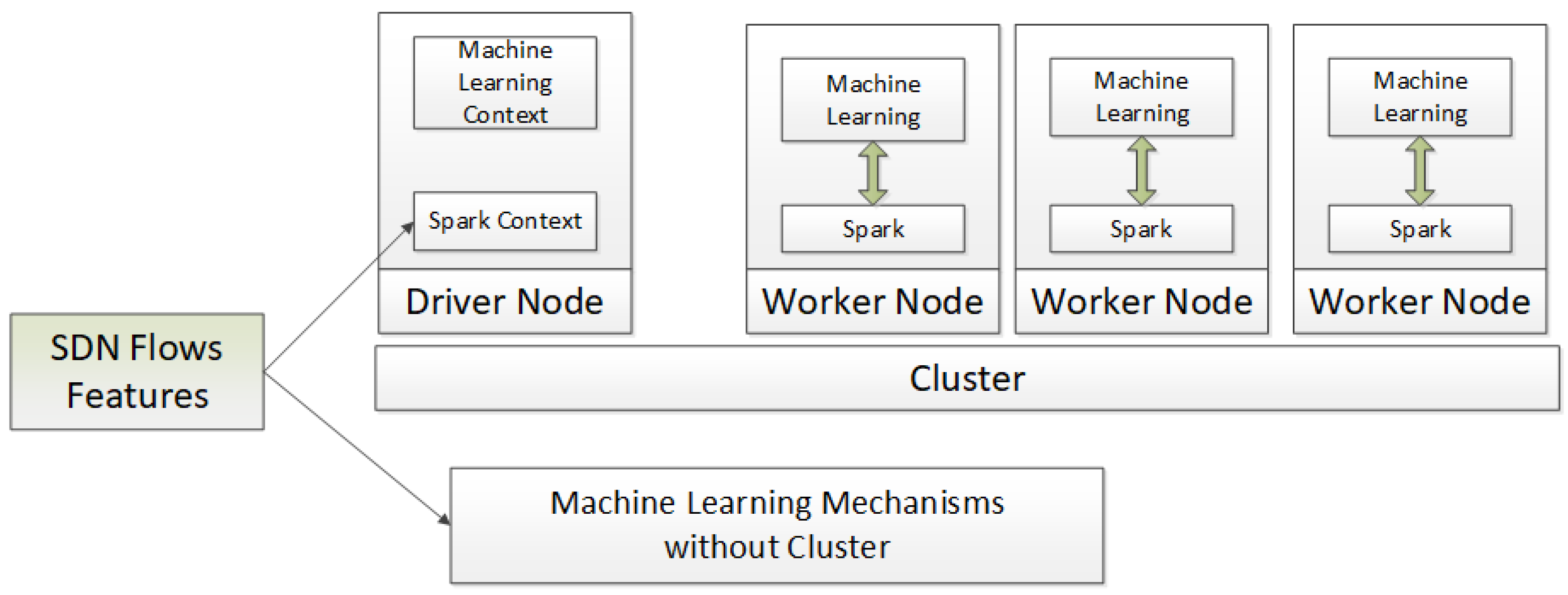
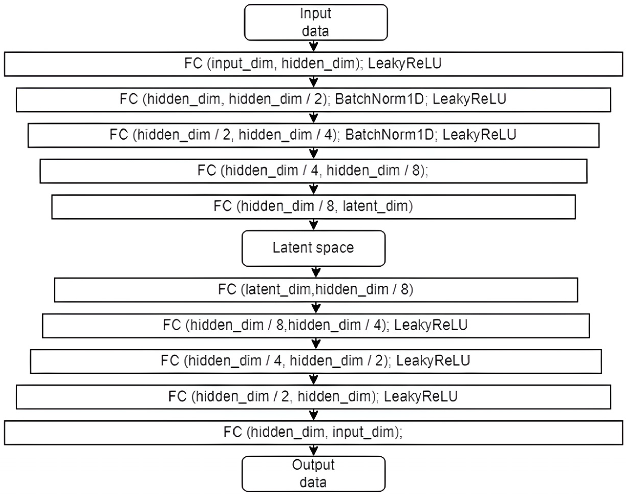
Disclaimer/Publisher’s Note: The statements, opinions and data contained in all publications are solely those of the individual author(s) and contributor(s) and not of MDPI and/or the editor(s). MDPI and/or the editor(s) disclaim responsibility for any injury to people or property resulting from any ideas, methods, instructions or products referred to in the content. |
© 2024 by the authors. Licensee MDPI, Basel, Switzerland. This article is an open access article distributed under the terms and conditions of the Creative Commons Attribution (CC BY) license (https://creativecommons.org/licenses/by/4.0/).