Research Progress and Engineering Applications of Viscous Fluid Mechanics

Abstract

This paper systematically reviews the development of viscous fluid mechanics and expounds the current research status of viscous fluid mechanics from the aspects of permeability experiments and research on viscous fluids, particle distribution and movement, droplet impact, modern computer technology simulation, etc. This paper summarizes the application status of viscous fluid mechanics theory in aerospace, fluid simulation, bioengineering, pipeline transportation, and other engineering fields, analyzes the influence of multiphysical field coupling, complex flow, and new materials on viscous fluid mechanics, and puts forward its development trend in algorithms, simulation, biomedicine, aerospace, and other fields.

1. Introduction

Viscous fluids are actual fluids with viscous properties, which are manifested by the nature of the fluid preventing its own flow, and this viscosity is caused by the interaction forces between the fluid molecules. As an important branch of fluid mechanics, viscous fluid mechanics studies the behavior and properties of fluids under the influence of viscous effects [1,2,3]. The most classical study is Newton’s assumption that the shear stress inside the fluid is proportional to the velocity gradient, thus introducing the concept of kinetic viscosity, which is applicable to many fluids in practical applications, such as water and air [4,5]. The formula and schematic diagram are shown below (Figure 1).

$$F=\mu {\displaystyle \frac{d_x}{d_y}}A,$$

(1)

However, in some engineering and natural phenomena, the viscous effects of fluids may significantly affect the kinematic properties of fluids, such as viscous hysteresis phenomena, the deformation and diffusion behaviors of fluids, etc. [6,7,8,9]. The study of viscous fluids is not limited to traditional Newtonian fluid models but also includes non-Newtonian fluids such as plastic, elastic, and viscoelastic fluids, which exhibit complex nonlinear behavior at high strain rates or high stresses. In addition to viscous fluids, viscous fluid theory also applies to fluids that are not viscous in nature (such as air, water, ethanol) which exhibit high viscosity when flowing in confined spaces (such as through membrane pores, porous materials, droplets hitting surfaces, etc.). Other relevant formulas and criteria for viscous fluid motion include the Froude criterion, Euler equation, N-S equation, Reynolds criterion, laminar flow, turbulence, turbulent flow, boundary layer theory, etc. [10,11].

In a wide range of fields of scientific exploration and engineering, many problems involve the permeability of viscous fluids moving on the surface or inside various materials and their specific modalities. For example, in the field of aircraft design, an in-depth understanding of the turbulence characteristics on aerodynamic surfaces and the potential impact of air viscosity on aircraft performance is essential [12,13]; in river engineering practice, an accurate assessment of the erosion of water flow on the riverbed and riverbank structures is equally indispensable [14]. In the pipeline transportation of chemical viscous liquids such as oil and liquefied natural gas, it is necessary to fully consider the potential impact of the viscosity of these liquids on the transportation efficiency [15]. To solve these problems, it is indispensable to use experiments and theoretical calculations to accurately determine various key parameters of viscous fluids [16]. In this paper, the basic theory, mathematical models, and practical applications of viscous fluid dynamics are systematically explored. This article summarizes the recent progress in the direction of experimental exploration and simulation research on the state of motion of viscous fluids, including the current problems and limitations. Meanwhile, the future development trend is envisioned, aiming to provide guidance and reference for research in the field of viscous fluid kinematic states.

2. Advances in the Study of the State of Motion of Viscous Fluids

Here are a few common ways to investigate the properties of viscous liquids and how they have evolved.

2.1. Experimentation and Research

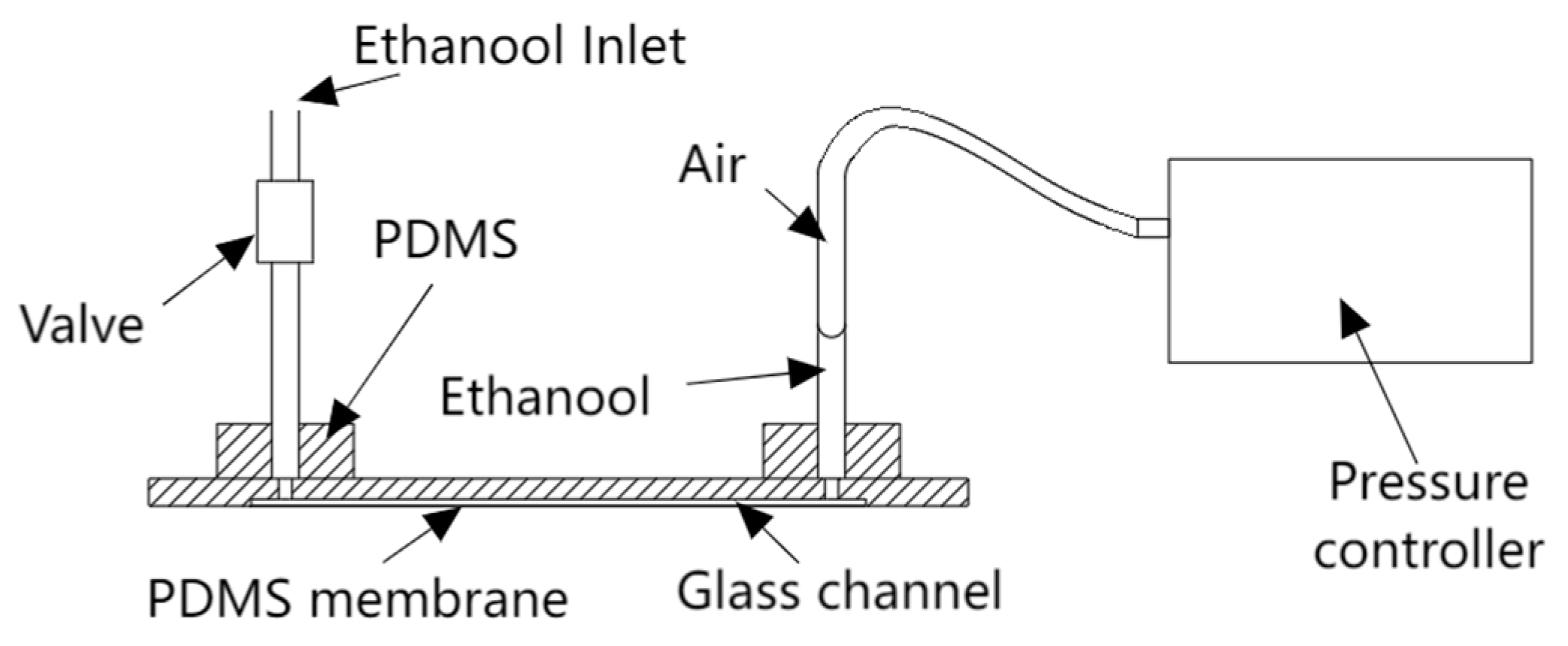
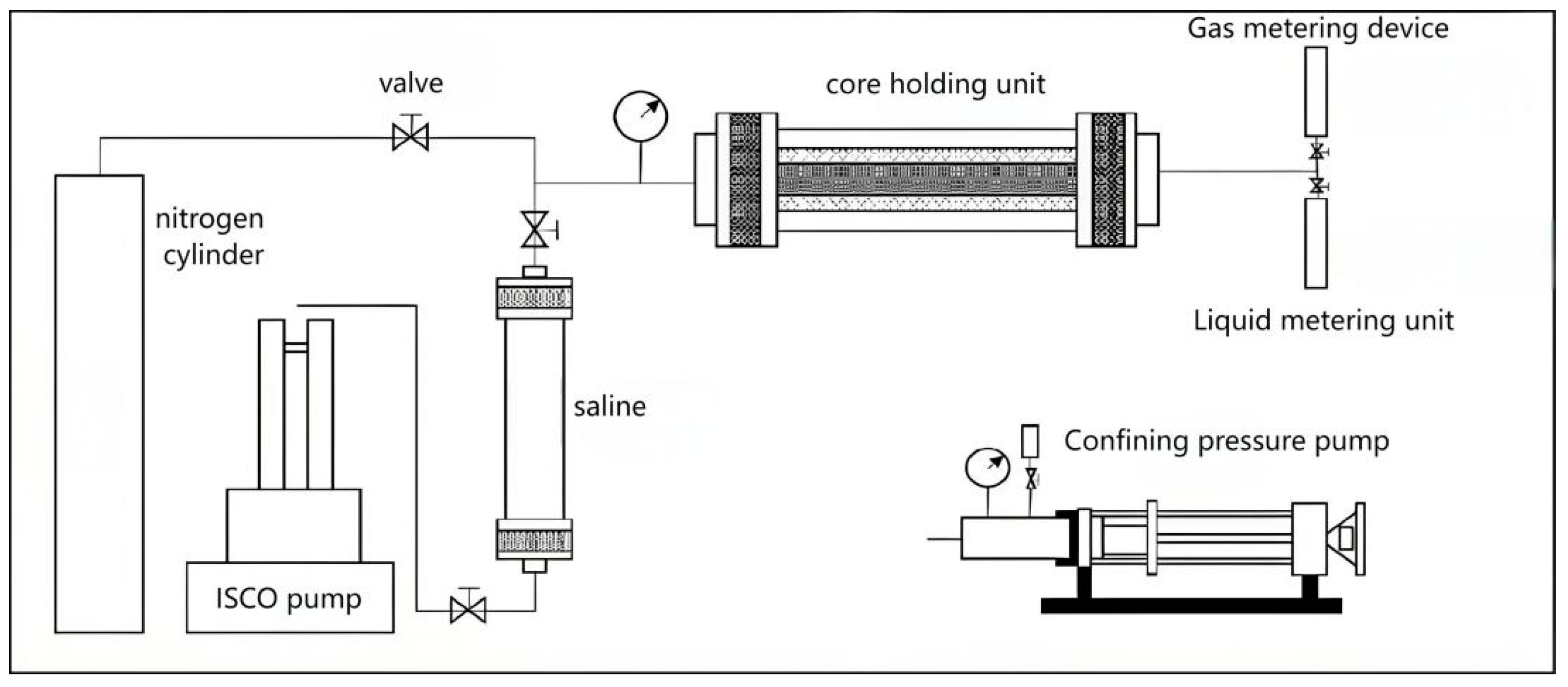
2.1.1. Experiments and Studies on the Permeability of Media to Viscous Fluids

Experiments and studies on the permeability of media to viscous fluids usually focus on investigating the permeability properties of fluids in porous media and their dynamic behavioral properties. Such studies have important applications in petroleum engineering, geology, civil engineering, and other fields [17,18,19]. The following are some common related contents and methods: (1) Porous media and permeability: porous media can be rocks, soils, rocks, or other materials in petroleum reservoirs. Their pore structure and connectivity determine the permeability of the media to the viscous fluid. (2) Permeability experimental methods: (i) the pressure-driven method (conventional method) involves applying a pressure difference to push the fluid through the porous medium, measuring the rate of fluid passage and pressure changes to calculate the permeability; (ii) the constant pressure method involves maintaining a constant pressure difference, measuring the rate of fluid permeation and permeability; and (iii) the resistance method involves determining the permeability properties by measuring the resistance of the fluid to passage through the porous medium. (3) The influence of the permeability of viscous fluids: the permeability properties of viscous fluids (e.g., petroleum, polymer solutions, etc.) are usually different from those of nonviscous fluids because viscosity affects the flow rate and distribution of the fluid. (4) Experimental equipment and techniques: permeability determination equipment (e.g., permeameters, permeability test benches, etc.) is used, usually in conjunction with pressure transducers, flow meters, and other instruments for accurate measurements. (5) Numerical simulation: Computational fluid dynamics (CFD) and numerical simulation methods are used to simulate the permeability behavior of viscous fluid in porous media and predict the permeability and fluid distribution of the medium to the viscous fluid [20,21,22,23]. These studies are important for optimizing oil extraction, groundwater resource management, environmental pollution prevention, and other fields and can help engineers and scientists to better understand and control the behavior of viscous fluids in complex media [24].

Currently, Darcy’s law and Forchheimer’s law are the main laws for determining the permeability of viscous fluids. Darcy’s law describes the relationship between the rate of permeation of a viscous fluid in a porous medium and the gradient of osmotic pressure under steady-state seepage conditions [25]. However, this law is mainly used for the determination of macroscopic permeability k under constant conditions, and it is questionable whether the fine channel changes under microscopic conditions affect this law. Forchheimer’s law as a model for describing non-Darcy’s flow is based on the overall average of the porous media model and does not take into account the specific effect of the microstructure inside the medium, which may limit its accuracy in some delicate porous media [26,27]. Both of these problems have been explored by researchers worldwide.

In this regard, Prof. Howard A. Stone et al. [28] of Princeton University carried out an experimental study on the pressure-driven passage of viscous fluids through a superelastic porous membrane. They fabricated their own experimental setup, which is schematically shown in Figure 2. The study focused on the permeability of thin PDMS membranes under convective conditions, and the experimental conclusions pointed out that macroscopic deformation can significantly affect the microstructure of soft materials and their transport properties.

Stafie, N, et al. [29] investigated the effect of polydimethylsiloxane (PDMS) cross-linking on the permeation properties of polyacrylonitrile (PAN)/PDMS nanofiltration (NF) composite membranes and found results that were inconsistent with the results of the swelling of the dense, This may be due to the lower pore intrusion rate of the composite film prepared at 10/2 compared to 10/1, or due to the heterogeneity of the silicone network. Delli, ML, (Delli, Mohana L.) et al. [30] investigated the change in permeability in a viscous material, natural gas-containing hydrate sediments, by a series of experiments, using different initial water saturations to reach hydrate saturations of up to 45% and measuring the corresponding fluid permeability during steady-state flow, which gradually decreases as the hydrate saturation increases.

Wang Shifang et al. [31] studied the spherical flow of Newtonian fluids in porous media based on fractal theory and technology. Three-dimensional spherical porous media percolation is widely found in hydrocarbon reservoirs. When only a small part of the reservoir is opened, the flow area has spherical radial flow, that is, the fluid flows from the center of the outward wellbore. The fractal permeability model of spherical porous media percolation is shown in Figure 3. The experiment reveals the physical mechanism affecting the spherical permeability and verifies the correctness of the fractal model of spherical permeability.

Wang Mang et al. [32] conducted an experimental study of the effect of different fluids and clay minerals on the permeability of rocks; the conclusions of their study showed that the nature of the viscous fluid itself has an influence on the macroscopic permeability of the permeable material, and the physical and chemical relationship between the fluid and the permeable material should also be considered along with the liquid permeability. The experimental device of media permeability to liquid designed by their research is shown in Figure 4. The experimental device provides a new experimental method for studying the permeability of viscous liquid.

Sun Weitao et al. [33] analyzed the complex fluid model of a tight reservoir and its applicability, using glycerol and methane gas for the pore structure of the tight reservoir at a micro- and nano-scale, and analyzed the theoretical basis and scope of application of the complex fluid model of the tight reservoir in detail. Their study concluded that the Cauchy correction model is a correction model used when the fluid does not meet the hydrodynamic characteristics of the continuous medium, and the Forchheimer model is a correction model that can be used when the fluid turbulence phenomenon is serious and its fluid flow still meets the hydrodynamic characteristics of the continuous medium. Ding Liang et al. [34], in order to study the permeability characteristics of non-homogeneous porous media, using high-temperature alloy-powder-sintered porous media as the experimental substrate, with pure air, water, and ethanol as the circulation medium, conducted an experimental study of the fluid through the porous media plate driving force and its movement characteristics of the relationship between the non-homogeneous porous media in the state of the single-phase flow of permeability characteristics. The experiments resulted in an obvious non-Darcy phenomenon, in which the viscous interaction between different fluids and the microporous solid wall is different, which may lead to the driving force required by high-viscous fluids being smaller than that of low-viscous fluids, resulting in inconsistency with the permeability determination of Darcy’s theorem.

In the above experiments on the study of Cauchy’s criterion and Forchheimer’s law for the permeability of viscous liquids, the conclusions generally agree that Forchheimer’s law is applicable to the case of non-Darcy flow, which is widely applicable, but it is relatively difficult to determine the parameters; Cauchy’s law of hydrodynamics has great difficulty in describing complex fluids and in obtaining experimental data, and Cauchy’s law will not be effective in the case of a change in microstructure due to deformation. With Cauchy’s law of hydrodynamics, it is very difficult to describe complex fluids and to obtain experimental data, and Cauchy’s law is invalid in the case of microstructures changed by deformation. The experimental method and experimental setup of the above experiments can provide a good idea for the subsequent related research, which is of great significance to promote the development of research on the permeability of viscous fluids.

2.1.2. Experiments and Studies on Droplet Impacts in Viscous Fluids

The study of viscous fluid droplet impact is an important branch in the field of fluid mechanics and surface phenomena, which involves the dynamic behaviors and physical processes of droplets in contact with solid or liquid surfaces under different conditions. These studies not only have far-reaching impacts on basic science but also have important implications in engineering applications. The dynamic process of droplet impact involves the deformation, expansion, and sputtering of droplets [35,36]. As a droplet approaches a surface, its shape is affected by surface tension, viscous, and inertial forces, which in turn affect the post-impact response. For example, higher surface tension and viscosity cause droplets to be more difficult to expand, which may cause droplet buckling or sputtering, while lower surface tension may contribute to droplets expanding more easily and forming a thin film. The phenomena of energy transfer and dissipation during droplet impact are also crucial [37]. Upon impact, energy is transferred between the droplet and the contacting surface, and some of this energy is either dissipated as heat or converted into the kinetic energy of the droplet, affecting the subsequent behavior and morphological evolution of the droplet. The understanding of these processes is particularly critical for engineering applications such as inkjet printing, coating technologies, and microfluidic system design [38,39]. The study of viscous fluid droplet impingement is also of direct practical relevance for solving problems in a variety of real-life and industrial applications. For example, in medical devices, understanding the expansion and adhesion behavior of droplets on various surfaces can help design more efficient fluid dispensing systems; in coating technology, controlling droplet impingement and expansion can improve the uniformity and quality of coatings [40]. Overall, the study of viscous fluid droplet impingement not only deepens our understanding of fluid dynamics and surface phenomena but also provides an important foundation and guidance for modern engineering technologies and applications.

The droplet impact velocity, angle, and impact energy have important effects on the experimental results. Too high or too low impact energy may lead to the atypical behavior of droplets or unrepeatable experimental results [41]. If the droplet cannot be fully wetted on contact with a solid surface or if there is a large contact angle, this will affect the deformation and rebound behavior of the droplet, making it difficult for the experimental results to accurately reflect the theoretical model [42]. Also, the Weber number of the liquid can greatly affect the collision results of viscous droplets [43].

With the development of technology and the increase in the demand for precise control, high-frame-rate high-speed video cameras for viscous droplet collision experiments to detect the experimental collision process, simulation software to simulate the collision process, and other methods of scientific research and investigation have been gradually and widely used [44,45,46]. For example, in the study of the impact of the Weber number on droplet collision, experimental controllable variables such as substrate elasticity, impact velocity, liquid viscosity, and liquid material can be systematically changed, and then, high-speed cameras can be used to clearly observe the phenomena of the diffusion, rebound, retraction, and wetting of droplets with different viscosities after impacting different substrates. By observing the experimental images, we can further study the influence of liquid viscosity on the critical rebound Weber number, maximum spreading, and contact time and speculate the mathematical model of the change in the Weber number before and after the collision [47,48,49]. In this line of thinking, Liu Hailong et al. [50], based on high-speed micro-digital camera technology and the establishment of the finite element numerical model of droplet impact on a superhydrophobic wall, carried out experiments to study the dynamic behavior of Newtonian fluid droplets with different viscosities (0.9–27.7 m Pa·s) impacting on a superhydrophobic wall (the static contact angle is 158°). Figure 5 shows the experimental process of the impact of Newtonian fluid droplets with different viscosity on the superhydrophobic wall captured by the high-speed camera when the We number is 28.2. It can be seen that the performance of the high-speed camera can observe a very clear droplet collision process.

On the issue that the impact velocity, angle, and impact energy of droplets have important effects on the experimental results, Chengyao Wang et al. [51] investigated the impact kinetic behaviors of water, anhydrous ethanol, and low-surface-energy droplets of different viscosities on hydrophobic surfaces through experimental visualization and explored and analyzed the effects of the three influencing factors, namely, the impact velocity, the surface wettability, and the droplet viscosity, on the impact kinetics of viscous droplets. The impact dynamics of viscous droplets were explored and analyzed. Qian Wenwei et al. [52] studied the impact process of viscous liquid and dense particle jets against a wall with a background of gasifier gasification technology and concluded that when the particle size is small, the dense particle impact flow shows a particle film morphology similar to the liquid impact; the higher the solid content rate, the lower the particle rebound probability and the more homogeneous the velocity and energy of the particles, which makes it easier to present the particle film morphology and other conclusions. In order to analyze the process of collision aggregation of unequally large droplets on walls with different wettability, Xing Lei et al. [53] prepared unequally large droplets with a volume ratio of 1:2 and carried out collision experiments in which small droplets on substrates with different wettability hit large droplets from different contact angles using high-speed camera technology to analyze the kinetic behaviors of droplet collision aggregation. The experimental device is shown in Figure 6, which provides a new idea of device construction for droplet collision experiments.

There exists the problem that the droplets cannot be completely wetted when contacting the solid surface, or there exists a large contact angle, which affects the deformation and rebound behavior of the droplets, making it difficult for the experimental results to accurately reflect the theoretical model. Zong Shaoqiang et al. [54] used a high-speed shadow imaging technique to investigate the evolution of viscous droplets (glycerol aqueous solution) impacting the drying and pre-wetting mesh surface to form liquid fingers and fragmentation and concluded that an increase in droplet viscosity and a decrease in mesh width would inhibit the complete penetration of droplets into the drying mesh surface and so on. Xing Lei et al. [55] used a high-speed camera to set up an experimental device to study the different changes in droplets impacting plates with different angles and humidity at different We numbers, and their experimental results provide some reference bases for complex fluid motion to a certain extent.

In addition to some droplet collision deposition and flight problems, researchers used viscous liquids of different materials and sprinkler heads of different specifications to simulate the spraying and collision process of viscoelastic fluid through experiments and observed the influence of viscoelasticity caused by the presence of polymers in the solution on the droplet deposition process and the influence of sprinkler heads on the atomization rupture of the solution with high accuracy [56,57].

In the above experiments, the construction of the experimental setup and the collection and prediction of the results are mostly based on the new century high-speed camera, which can instantly turn the droplet collision into thousands of frames for the researcher to study the mechanism of droplet collision in a more detailed and accurate way. Therefore, high-speed cameras play an important role in the study of viscous liquids and the motion of some other fluids.

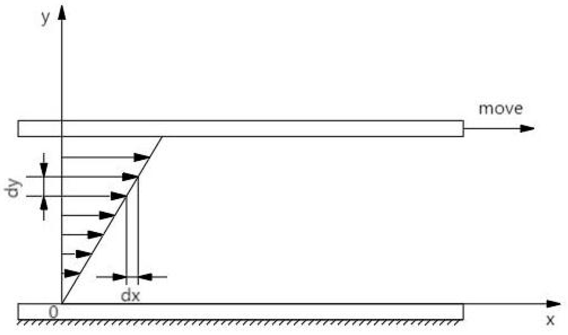
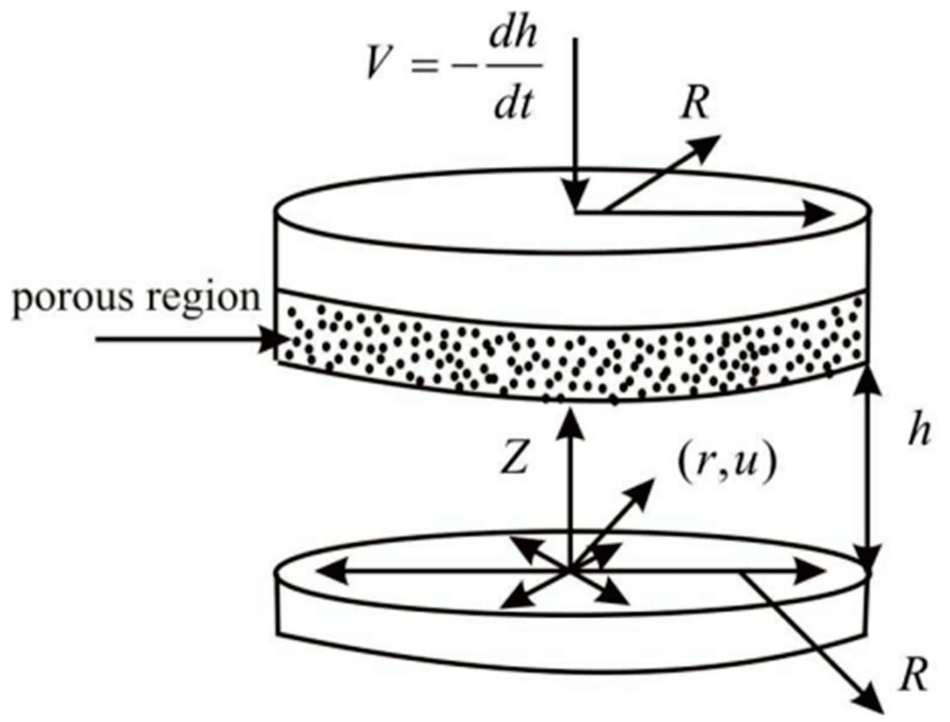
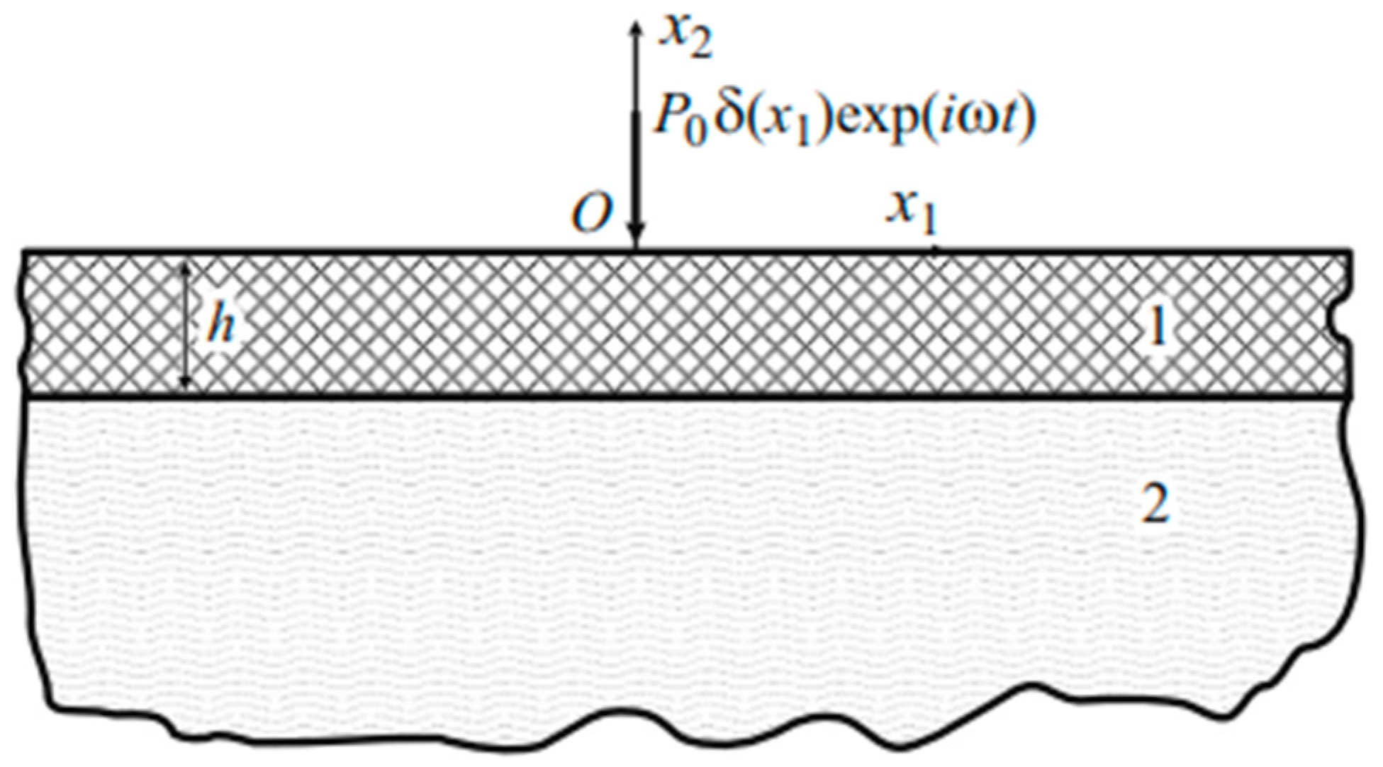
2.1.3. Experiments and Studies on the Flat-Plate Gap Method

The flat-plate gap method for viscous fluids is an important experimental method for investigating the properties of viscous fluids flowing between two parallel solid surfaces. This traditional experiment not only reveals the behavior of the fluid at the microscopic scale but also measures important parameters such as its rheological properties and viscosity [58]. In the experiments of the flat-plate gap method for viscous fluids, it is first necessary to prepare two parallel solid surfaces, usually flat plates or pipe walls. The flatness of these surfaces has an important effect on the experimental results, so high-precision experimental equipment is usually used [59,60]. Next, an appropriate sample of viscous fluid is selected for the experiment. The choice of viscous fluid can be determined according to the specific purpose and requirements of the experiment [61], e.g., fluid samples with different viscosities and different rheological properties can be selected. While the experiment is in progress, a small gap, usually between a few micrometers and a few millimeters, is set between two flat plates. The size of this gap will directly affect the flow characteristics of the fluid therein. The fluid can be guided to flow in the gap by applying some pressure or by applying an electric field (for galvanic fluids) [62,63]. During the experiments, the flow data of the fluid in the gap are obtained by means of appropriate measuring devices such as pressure transducers, flowmeters, or laser measuring devices. The commonly measured parameters include the flow velocity distribution, shear stress distribution, and pressure distribution of the fluid [64,65,66].

The measurement of these data is important for inferring the viscosity, flow resistance, and flow behavior of viscous fluids in confined spaces, but this experimental method has the problems that the control of experimental conditions requires high-precision equipment and operating techniques, and the stability of experimental environments is highly required. Therefore, Prausová, H, et al. [67] investigated the laminar, turbulent, and transitional flow regimes of a viscous fluid in a narrow gap between two substrates with a parallel distance of 2 mm and obtained the static and stagnant pressure ratio distributions along the axis of the channel using both optical and gas-dynamics methods. Christensen, AH, et al. [68] developed a mathematical model to investigate the flow behavior of viscous fluid in a narrow gap between two rectangular elastomeric plates with a distance of 2 mm. The model is based on low-Reynolds-number fluid dynamics and linear plate theory, and it is concluded that the outflow volume of a viscous fluid increases linearly with increasing pressure. Lin, JR, et al. [69] investigated the combined effect of the properties of viscous liquids subjected to pressure as well as non-Newtonian coupled stresses by developing a mathematical model of piezoelectric-viscous dependence and non-Newtonian coupled stresses in a wide parallel rectangular-plate extruded membrane based on Stokes microcontinuum medium theory and incorporating factors related to the variation in viscosity with pressure. Vijayakumar, B, et al. [70] designed a set of mathematical models based on the Cartesian coordinate system for the effects of piezo-viscous dependence and non-Newtonian coupling stress on the performance of cylindrical-perforated-plate extrusion-film bearings. The digital model is shown in Figure 7.

Neufeld, JA, et al. [71] studied the diffusive motion patterns between a thin film of viscous fluid and a thin elastomeric sheet on a plate by extrusion using a permeable horizontal plate and showed that an air gap forms underneath the viscous fluid as it is extruded through the plate until the fluid re-flows onto the plate. For very light or stiff elastic sheets, the air gap contacts may extend well beyond the fluid discharge zone. Zamanov, AD, et al. [72] envisioned a fluid viscoelastic model consisting of a viscoelastic plate and a half-plane filled with a viscous fluid, which is shown schematically in Figure 8. Using the exact equations of viscoelastic dynamics for describing the motion of the plate and the linearized N-S equations for describing the fluid flow, the problem of forced vibration of the system under plane strain was investigated.

As can be seen from the above researchers’ studies on the motion of viscous fluids between plate gaps, this type of experiment is complicated by the experimental setup, so much so that most of the researchers use digital models for predictive studies. In terms of scientific research, this approach helps to gain a deeper understanding of the flow properties of viscous fluids at the microscopic scale, explore the complex rheological behavior of fluids, and save experimental costs. In engineering applications, this digital model prediction method can provide important data support for designing viscous fluid lubrication systems, optimizing fluid transport pipelines, and so on.

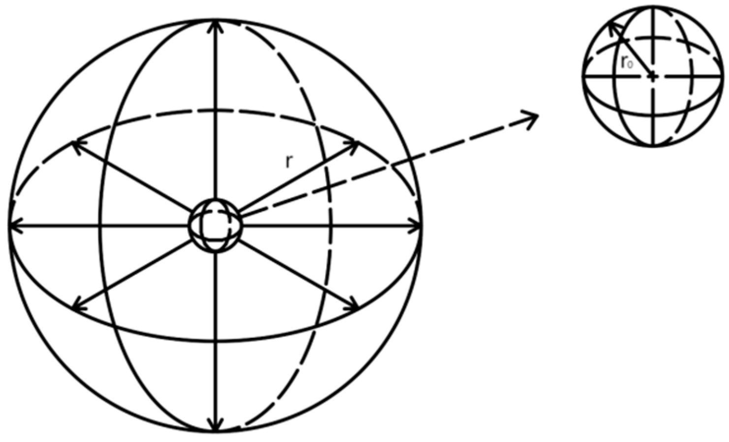
2.1.4. Experiments and Studies on the Oscillation Method

The viscosity of a fluid is measured or its state of motion is studied using an oscillating-disk- or oscillating-cylinder-type geometry or by external shock conduction, which is inferred from the frequency of the oscillations and the response of the oscillator. The basic principle is to use external excitation to cause oscillations within or on the surface of the fluid and to reveal the fluid’s hydrodynamic behavior and oscillatory modes by observing and analyzing the oscillatory phenomena [73,74]. This method is commonly used to study polymer solutions or complex liquid systems containing additives [75]. As a research tool, the viscous liquid oscillation method, although it has an important role in fluid dynamics and engineering applications, has some potential problems and challenges, which include complex fluid behavior and nonlinear effects, difficulties in ensuring the control and stability of the experimental conditions, the large amount of resultant data requiring complex data processing algorithms and technical support, and the lack of a precise interpretation for the phenomena of liquid oscillations that have been observed and recorded, which makes the exact interpretation and physical significance of the different oscillation modes difficult to analyze [76,77,78].

The results of oscillations of single geometries in the experiments of the oscillation law of viscous fluids often do not allow a clear determination of the exercises between the two. Nuriev, AN, et al. [79] studied the low-amplitude and high-frequency oscillations induced by the reciprocating motion of ellipsoidal cylinders with different axial ratios in viscous fluids based on the law of harmonics, and the limits of the asymptotic theory were determined through the observation of oscillations of the surface of the liquid, which is more diverse than the study of the oscillatory behavior of individual geometries in viscous liquids. In addition to the study of viscous liquids using geometries probed into the liquid to produce displacements or oscillations, the use of acoustic waves to impart oscillations to the liquid is a very worthwhile research method. In view of this problem, Kremer, J et al. [80] implemented non-contact positioning suspension of viscous liquids such as silicone oil and propanol based on acoustic suspension, and placed them under the same ambient pressure to measure the surface tension and viscosity of each liquid. The construction diagram of the experimental device is shown in Figure 9.

Brenn, G, et al. [81], based on the transient deformation induced by oscillation, built an experimental setup and predicted and analyzed the small-amplitude axisymmetric-shape oscillations of a viscoelastic droplet suspended in a gas and improved the Jeffreys model to obtain a new characteristic equation for the complex frequency, which quantifies the effects of the two time scales, stress relaxation and deformation delay time, on the oscillatory behavior of the droplet. Due to the traditional experimental research method of building physical platforms having many inconveniences, such as the stability being difficult to control and the experimental results being difficult to obtain, many researchers use computer technology to digitize the physical environment of the object of study in order to control the variables, and the digital simulation makes it easy to extract the results. Feng, L, et al. [82] took into account the emergence of severe precession and frequency shifts in experiments in the measurement of the surface tension of liquid introducing non-negligible measurement errors in the determination, so the effects of the oscillation amplitude of viscous droplets and the viscous effect on the droplet oscillation were investigated by three-dimensional modeling simulation. The modeling and simulation are shown in Figure 10 and Figure 11.

The research methods introduced above have mainly covered three research methods, i.e., the traditional contact oscillation method, the non-contact oscillation method, and the digital simulation method. Each of the three methods has its own advantages and shortcomings, and the following

Table 1. Comparison of research methods for viscous fluids.

Method	Cost	Accuracy	Time Consumption	Future Development Potential
Conventional contact shock method	High	Relatively low	High	Low
Non-contact oscillation method	High	Moderate	High	Relatively low
Digital simulation method	Low	High	Low	High

makes a simple comparison between these methods for the readers to refer to.

When conducting relevant experiments, researchers should consider factors such as money, time, and target results for research exploration. However, I think that with the development of computers, simulation will be the mainstay of research methods in the future. The table showing the comparison between the traditional physical experiment method and the computer simulation method is also of reference significance for the previous several summaries.

2.2. An Investigation of the Simulation of the State of Motion of Viscous Fluids by Modern Computer Technology

The phenomenon of viscous liquid fluid exists widely in nature, daily life, and industrial production, and since ancient times, scientists have never stopped investigating the process of viscous fluid motion. In the 21st century, with the significant improvement of computer computing power, the application of computer and general software to simulation analysis of fluid dynamics, a new fluid motion research method, has become popular [83,84]. This kind of software adopts numerical computation methods programmed to directly solve the flow master equations (e.g., Euler’s equations or Navier–Stokes equations) in order to reveal the laws of various flow phenomena. They integrate the knowledge of various disciplines such as mathematics, physics, computer science, fluid mechanics, 3D modeling, scientific visualization, etc., and the simulation methods are mainly classified into mesh and meshless methods [85,86]. At present, the mainstream fluid simulation and meshing software and algorithm programs include ANSYS Fluent, MATLAB, FEM, MST, Flo EFD, AICFD, Polyflow, RealFlow, AcuSolve, XFlow, PowerFLOW, VirtualFlow, Flowmaster, etc. These fluid simulation software and algorithms cover a wide range of applications from 2D model simulation to 3D model simulation [87,88,89]. Scientific researchers simulate and analyze the motion process of fluids based on mathematical models or three-dimensional physical models, which are more efficient, accurate, and intuitive compared to the pure mathematical computation method of predicting fluid motion in the last century, which provides a certain theoretical basis for the judgment of the motion phenomena of viscous fluids and has become an important method of research on fluid-related motion [90,91,92].

2.2.1. Computerized Algorithmic Solution of Viscous Fluids

Currently, many scientists use computers to compile algorithmic programs to help them find the relationship between various variables from the huge amount of experimental data and at the same time set the program to iterate autonomously through the computer, and the computational speed far exceeds that of the original handwritten calculations. Mentzoni et al. [93] proposed an oscillatory flow condition relevant to marine applications based on the Navier–Stokes equation. A two-dimensional viscous flow field model for porous-plate hydrodynamics was developed and analytically solved using MATLAB, and the accuracy of the model was experimentally verified. Kyung Hyun Ahn et al. [94] investigated the particulate system of solid particles suspended in a viscoelastic medium based on a novel numerical algorithm of the lattice Boltzmann method (LBM). Zhu Liang et al. [95] used the Giesekus model of viscoelastic fluid and spherical rigid particles as the research object and used the quasi-constant algorithm based on the relative motion model to investigate the distribution characteristics of the lateral lift force of the particles in the channel; the computational model is shown in Figure 12.

Hanqing Li et al. [96], for Oldroyd-B-type viscoelastic fluid, used the lattice Boltzmann method (LBM) to obtain the flow field distributions of the viscoelastic fluid in the dilatational and constrictive flow paths (the flow paths are shown in Figure 13) and numerically analyzed the settling process and characterization of the particles in dilatational and constrictive flows based on the point-source particle model.

Different from the forward algorithm which is based on using known conditions to obtain unknown results, Tsepelev, IA, [97], with the final state of the target fluid being highly viscous and incompressible, used algorithms to deduce the unknown initial state of the fluid in reverse, using OpenFOAM software based on linear algebra to develop a new iterative algorithm in reverse, with the computational error and input data error on the opposite side. Xu, XY, et al. [98] improved the SPH algorithm in order to simulate the transient free-surface flow of viscous and viscoelastic fluids, which improved the accuracy and stability of the algorithm. It can accurately and stably simulate the flow and oscillating pressure field at the free surface of viscous and viscoelastic fluids, which provides a more efficient method for the study of numerical algorithms for viscous fluids.

2.2.2. Simulation of Viscous Fluid Motion by Computer Techniques

In addition to the use of advanced computer technology for the numerical calculation of the model of the fluid, we can also use simulation software to model the target fluid environment so that the resulting results contain static and dynamic processes and a series of numerical values and plots, which can be more intuitive for researchers to understand the process of fluid motion [99]. The basic solution process is as follows: Firstly, the continuous fluid dynamics equations (e.g., the Navier–Stokes equations) are discretized into discrete points or cells using finite difference, finite volume, and finite element methods, which are common discretization methods, so that they can be processed by computers [100,101]. This is followed by the selection of appropriate time integration methods (e.g., explicit or implicit methods, Runge–Kutta methods, etc.) that allow the computer to solve the fluid dynamics evolution over time. These methods take into account stability and accuracy, especially for nonlinear and unsteady flows. The fluid region then needs to be divided into discrete cells or grids according to the geometry and boundary conditions of the fluid domain, and the grid density or local encryption, grid type selection, etc., are set according to the size and needs of the model [102,103,104]. An example is shown in Figure 14, which provides a simple reference for your understanding. The figure is a two-dimensional model of a pipeline. After setting the entrance, exit, and wall surface, dividing the grid, and setting various physical fields and load conditions, simulation can be performed.

Finally, appropriate iterative solvers (e.g., conjugate gradient method, stability iteration method, etc.) are to be used to solve the discretized fluid dynamics equations. These methods usually take into account the nonlinear, viscous, and inertial properties of the fluid [105]. Of course, the correct treatment of boundary conditions is crucial when computing fluid dynamics. This includes the setting of velocities, pressures, or other physical quantities at the boundary of the fluid flow to ensure the accuracy and physical soundness of the numerical solution [106]. For larger models, more complex structures, or simulation environments for fluid simulation, it is also necessary to reasonably allocate the number of computer running cores for the solution in order to prevent insufficient arithmetic power leading to the inability to give simulation results after a large number of time iterations [107].

As far as simulation technology in the study of viscous fluid motion is concerned, Xu Baiping and others [108] used the transient finite element method (FEM) combined with the mesh superposition technique (MST) with high-viscosity Newtonian fluid as the object of study, using numerical simulation methods to study the mixing motion process of viscous fluid in a cavity under the action of triangular rotor mixing with different staggered column angles, and the simulation image is shown in Figure 15.

Liang Yuanfei et al. [109] investigated the turbulence damping rate of viscoelastic fluid for wall turbulence of up to 18.9% by building a three-dimensional computational basin for simulation operations through OpenFOAM, and the results of the power spectral density showed that the energy attenuation of the viscoelastic flow was slower than that of Newtonian fluid. Kaiyuan Shi et al. [110] proposed a fully nonlinear potential flow method, the spectral coupled boundary element method (SCBEM), to address the problem of limited fluid computational resources. Compared with the traditional BEM method, the algorithm speed is greatly improved by using the region decomposition method. The numerical results also confirm the validity and accuracy of the simulation results. Zhu Yafei et al. [111] took the binary viscous fluid as the main research object, visualized and analyzed the flow diffusion behavior of two viscous fluids, hemolysate and hematoma, through the multiphysics field simulation software COMSOL Multiphysics, and improved and designed medical drainage tubes according to the visualization results. Shen Yang et al. [112] established a relative motion model to understand the effect of the shear thinning effect on the particle motion in viscoelastic fluid; a simulation of the mesh division and the vector diagrams are shown in Figure 16 and Figure 17. The results show that under the influence of a shear thinning effect of different Weber numbers, the elasticity of the viscoelastic fluid is reduced, leading to the movement of particles to the outer wall.

Qiu, LC, et al. [113] applied projection-based incompressible smooth particle hydrodynamics (ISPH) to the simulation of the deformation process of a viscous droplet, and the simulation results showed that projection-based ISPH with the particle displacement technique can be used to simulate the deformation process of a viscous droplet stably and accurately.

In general, the visualization of the simulation technology to make the original only rely on the formula deduction and imagination of the viscous fluid exploration and understanding of the process has become a vivid image and more intuitive, very powerful in promoting the development of fluid mechanics. However, the computational power of the computer is a major obstacle to the simulation, and the future development of viscous fluid exploration will inevitably accompany the development of computing power and progress.

At the end of this section, this paper provides a comparison of the characteristics between algorithms and simulations for researchers’ reference. Algorithms and simulations each have their own unique strengths and limitations, as shown in

Table 2. Comparative table of advantages and limitations of algorithms and simulations.

Method	Precision of Mathematical Results	Visualization	Time Cost	Complexity Adaptability
Arithmetic	High	Mediocre	Relatively low	Low
Emulate	Relatively low	First-rate	High	High

, and an understanding of their characteristics and applicability scenarios can help in choosing the most appropriate tools and methods for solving viscous-fluid-related engineering or scientific problems.

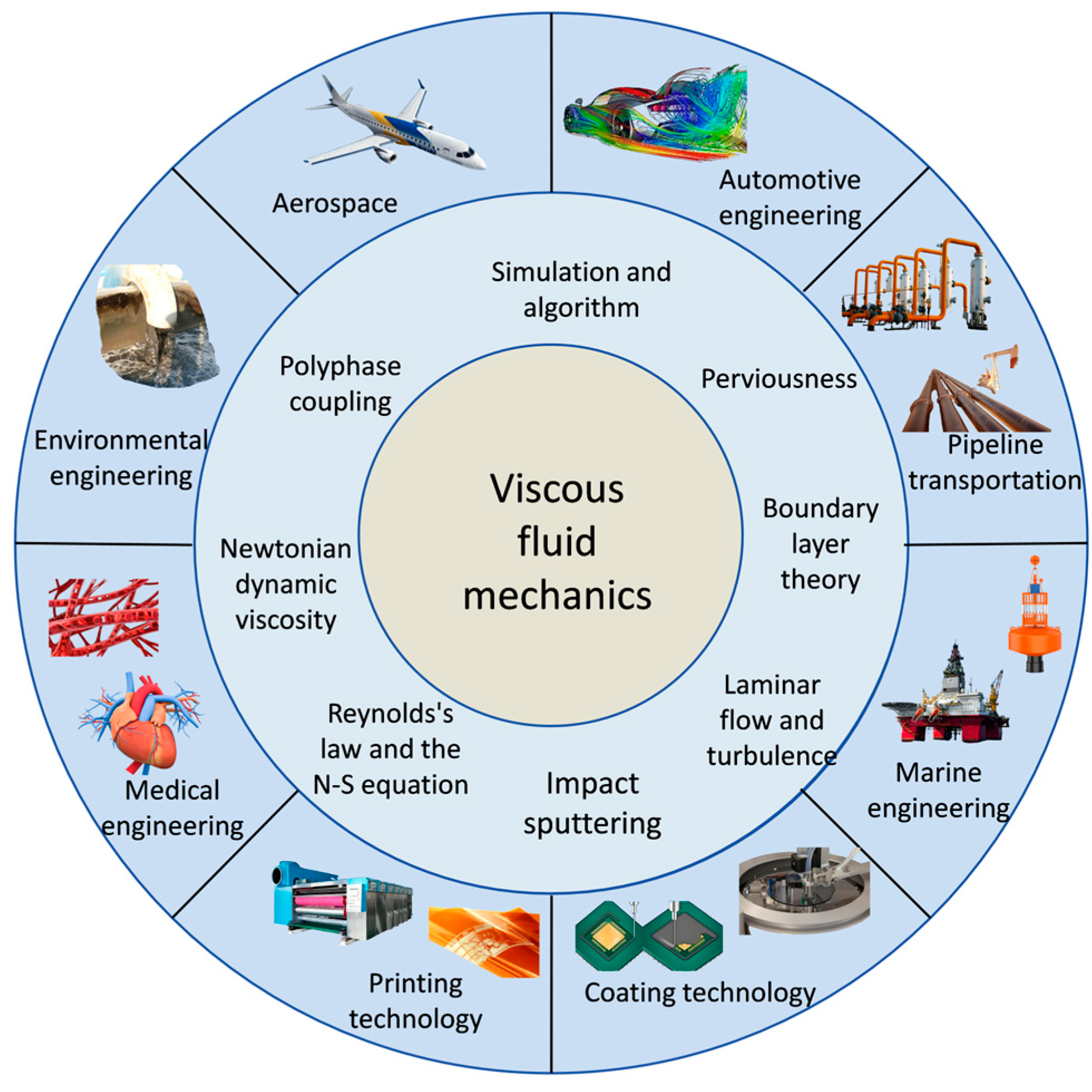
3. Application Areas of Engineering

The theory of viscous fluid dynamics (or simply viscous fluid theory) plays a crucial role in the field of engineering. The theory not only provides engineers with tools to deeply understand and predict the behavior of various fluids but also directly contributes to the development of several industries in design, optimization, and innovation. In aerospace engineering, the theory of viscous hydrodynamics is of crucial importance for designing the aerodynamic shape of aircraft and optimizing airfoils [114,115]. Through the in-depth study of viscous fluid dynamics, engineers are able to gain a deep understanding of aerodynamic effects such as aerodynamic drag and lift generation mechanisms. This knowledge helps to optimize the aerodynamic shape of the vehicle, reduce drag, improve flight efficiency, reduce fuel consumption, and thus extend range [116,117,118]. In automotive engineering, viscous fluid dynamics theory is widely used to improve the aerodynamic performance of vehicles. By gaining a deeper understanding of the complexity of air flow during vehicle operation, engineers can design and optimize body shapes, mirrors, and other streamlined components to reduce air resistance and improve the fuel efficiency and driving stability of vehicles [119,120]. In marine engineering, the theory of viscous hydrodynamics is used to study the hydrodynamic performance of marine structures (e.g., platforms, buoys, etc.). By analyzing the motion characteristics of water flow on the surface of structures, engineers can optimize the design to improve the stability and wind and wave resistance of the structures to ensure that they can operate safely in extreme marine environments [121,122,123]. In the oil, gas, and chemical industries, the theory of viscous fluid mechanics plays an important role in the design and optimization of piping systems. Engineers need to have an in-depth understanding of the flow characteristics of fluids within pipelines to minimize energy loss, control pressure drops, avoid pipeline clogging, and ensure the stable and efficient transportation of fluids [124,125,126]. In biomedical engineering, the theory of viscous fluid dynamics is important for studying the flow of blood in the cardiovascular system. For example, in the simulation model of heart valves, viscous fluid dynamics can simulate the flow of blood over the valves and evaluate the hydrodynamic properties of the valves when they open and close, which can help optimize the design and surgical plan of artificial heart valves [127,128,129]. In industrial production, the theory of viscous hydrodynamics is used to improve the efficiency and quality of coating technology and printing engineering. By precisely controlling the droplet impaction, expansion, and drying processes, engineers can improve the uniformity and durability of coatings, which in turn affects the final quality and appearance of the product. This theory has a wide range of applications in fields such as electronics and packaging materials [130,131]. In environmental engineering, the theory of viscous hydrodynamics is applied to the design of wastewater treatment systems and water management programs. Through a deeper understanding of the complex behavior of water flow in the treatment process, engineers can optimize the design of treatment facilities, improve the treatment efficiency, and reduce the impact on the environment, thus protecting water resources and the ecological environment [132,133,134]. As shown in Figure 18, this paper provides a schematic diagram of engineering application for readers’ reference, which includes some research directions and the applications of related technologies involved in viscous fluid mechanics in the engineering field. The applications in aerospace, fluid simulation, bioengineering, pipeline transportation, and other engineering fields in the figure correspond to the above.

In summary, the wide application of viscous fluid dynamics theory in the field of engineering not only provides an effective means to solve complex fluid dynamics problems but also greatly promotes the technological progress and innovation in various industries. With the continuous development of science and technology and increasingly diversified engineering needs, the research and application of viscous fluid dynamics will continue to play a pivotal role in various fields, providing engineers with a solid theoretical foundation and powerful technical tools to help them cope with a variety of challenges and promote the continuous development of engineering technology.

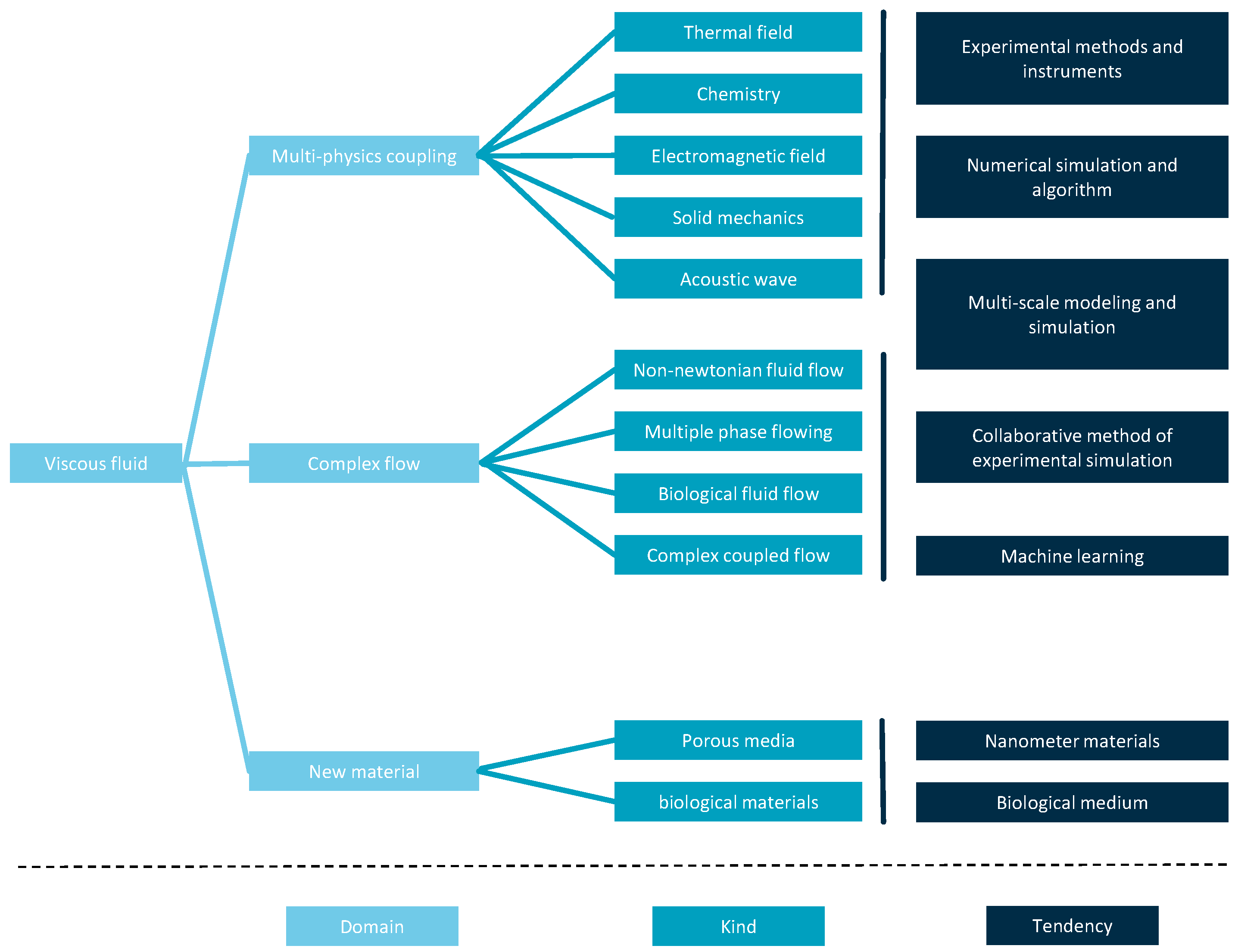
4. Future Trends and Directions

Viscous fluid mechanics, as an important branch of fluid mechanics, has made remarkable progress in the past decades and has been widely used in several engineering and scientific fields. The future research and development outlook can be viewed from the following aspects (Figure 19):

(1)

Future research in viscous fluid mechanics will pay more attention to the coupling of multiple physical fields. The physical fields and their effects that need attention include the following: (1) Thermal field: Temperature changes can significantly affect the viscosity of the fluid; usually, a temperature increase will lead to a decrease in the viscosity of the fluid, while a decrease in temperature will increase the viscosity. This coupling is particularly important in high-temperature lubrication and polymer fluid handling. (2) Chemical reactions: Chemical reactions can change the composition of a fluid and thus affect its viscosity. For example, cross-linking reactions in polymer fluids can lead to nonlinear changes in viscosity, which is critical for the processing and control of viscoelastic materials. (3) Electromagnetic fields: Magnetic fluids can produce morphological changes and controlled flow behavior under an applied magnetic field, such as electromagnetically driven fluids in liquid metals. This coupling can have applications in liquid metal metallurgy, aerospace technology, and biomedical sensors. (4) Solid mechanics: in fluids in contact with solid walls, the morphology and roughness of the solid surface can significantly affect the friction and adhesion behavior of the fluid.(5)Acoustic effects: Acoustic fields can affect the viscoelasticity and flow properties of fluids, for example, in the ultrasonic acoustic field for microfluidic manipulation and in biomedical imaging. This coupling helps to control the mixing and stirring process of microfluidics; not only limited to the above physical fields, or even using two or more kinds of physical fields coupled together, numerical simulation or complex experimental methods can be used in studies and analysis in order to add a comprehensive, in-depth understanding of complex engineering phenomena and natural phenomena. This multiphysical field coupling research method is expected to provide new ideas and solutions for innovations in the fields of energy conversion, environmental protection, and biomedicine. I believe that the optimization trends in this area are as follows: (1) for complex systems and phenomena, such as biofluids, multiphase flows, and non-Newtonian fluids, multiscale modeling and simulation methods should be improved to capture the details in different spatial and temporal scales; (2) for numerical simulation, new numerical simulation techniques and algorithms such as mixed-element methods, implicit-coupling methods, and adaptive mesh techniques should be improved to facilitate the numerical modeling and analysis of complex fluid systems;(3)experimental techniques, such as microfluidic experimental platforms and advanced imaging techniques, should be improved to further improve the precision of experimental device components and optimize real-time sensing techniques, which can more accurately validate theoretical models and numerical predictions.

(2)

One of the future research priorities will be the in-depth understanding and control of complex flow phenomena. Viscous fluid complex flow phenomena include the following: (1) non-Newtonian fluid flow: non-Newtonian fluid flow is not only affected by the velocity gradient but may also be affected by the non-uniformity and time-dependence of the flow field, resulting in complex flow behaviors, such as shear thinning and shear thickening phenomena; (2) multiphase flow: this refers to the simultaneous presence of two or more substances (e.g., gases, liquids, or solid particles) of the flow system, with a focus on gas–liquid, liquid–liquid, solid–liquid, and other combinations of flow, such as foam flow, bubble flow, the movement of particles in suspension, etc.; (3) biological fluid flow: the flow mechanism of blood flow in living organisms and fluid exchange across the walls between cells is very complex, and in the future, it may be possible to simulate blood flow, intercellular fluid exchange, and other biophysical fluid dynamics phenomena, which will aid in the diagnosis of diseases, the research and development of new drugs, and bioengineering; and (4) complex coupled flow: complex coupled flow mainly refers to those flow phenomena that are not only affected by the flow characteristics of the fluid itself but are also affected by the interaction between the fluid and the solid, the fluid and the electric field or magnetic field, etc., for example, electromagnetic fluids (such as plasma), magnetic fluids (such as magnetorheological fluids), and complex fluid systems that interact with particles. I think there are several optimization trends in this area: (1) data-driven method: using machine learning and data mining techniques to process a large amount of experimental data and numerical simulation data, such as the bird flocking algorithm and the whale algorithm in machine learning, to discover the patterns and laws in the flow and optimize the parameters and boundary conditions of the numerical model to improve the accuracy and efficiency of the simulation results; (2) experimental simulation synergistic method: comparing and verifying the experimental data with the numerical simulation results and continuously improving the numerical model to enhance its applicability and realism in complex flow systems; In addition to this, we can also can deepen the research on microscale flow, boundary layer control, wake phenomena, etc. By deepening the understanding and control of these complex flow phenomena, we can provide strong support for the innovation and development of related fields.

(3)

The development of viscous fluid mechanics will also be closely related to the application of new materials. This area currently has significant trends in the following areas: (1) Porous and complex media: with the deepening of the study of fluid mechanics in porous media, new porous materials (such as 3D printed structures) and complex media (such as nanomaterials) could be developed, and these materials may exhibit nonlinear, non-Newtonian flow properties, requiring new numerical simulation and experimental techniques to understand their flow behavior, for example, the permeability of the material, the surface tension and viscosity of liquid nanomaterials, etc. (2) Biomaterials: The field of biofluid dynamics has an increasing demand for research on biomaterials (e.g., soft tissues, cell membranes, etc.), and the characteristics of these materials may lead to complex flow behaviors, which need to be combined with experimental and simulation methods to conduct an in-depth study. In this regard, I’m more optimistic about the potential of nanotechnology in the study of viscous fluids, and we need to actively explore how to utilize new technologies such as nanotechnology to change the viscosity and surface tension of fluids and develop new fluid control and regulation technologies to meet different engineering needs and challenges.

As a rapidly developing field, future research in viscous fluid dynamics will continue to explore the nature of complex fluid phenomena in depth. By combining advanced computational techniques and interdisciplinary research methods with highly sophisticated camera technology, control technology, detection technology, etc., viscous fluid dynamics is expected to promote applications and innovations in many fields, such as engineering, science, and medicine, and provide more accurate and effective theoretical and methodological support for solving practical problems.

References

1. Romatschke, P. New developments in relativistic viscous hydrodynamics. Int. J. Mod. Phys. E 2010, 19, 1–53. [Google Scholar] [CrossRef]
2. Phillips, T.N.; Roberts, G.W. Lattice Boltzmann models for non-Newtonian flows. IMA J. Appl. Math. 2011, 76, 790–816. [Google Scholar] [CrossRef]
3. Aharonov, E.; Rothman, D.H. Non-Newtonian flow (through porous media): A lattice-Boltzmann method. Geophys. Res. Lett. 1993, 20, 679–682. [Google Scholar] [CrossRef]
4. Hu, H.; Zhang, G.; Zhao, T. Overview of computational fluid dynamics and discrete element coupling methods. In Proceedings of the 5th China Symposium on Hydraulic and Hydropower Geotechnical Mechanics and Engineering, Yichang, China, 17–21 September 2014; p. 4. [Google Scholar]
5. Liu, Y.-Z. Overview of dynamic research methods for liquid-filled rigid bodies. Mech. Pract. 2015, 37, 397–400. [Google Scholar]
6. Silva, D.P.; Coelho, R.C.; Pagonabarraga, I.; Succi, S.; da Gama, M.M.T.; Araújo, N.A. Lattice Boltzmann simulation of deformable fluid-filled bodies: Progress and perspectives. Soft Matter 2024, 20, 2419–2441. [Google Scholar] [CrossRef] [PubMed]
7. Coussot, P. Yield stress fluid flows: A review of experimental data. J. Non-Newton. Fluid Mech. 2014, 211, 31–49. [Google Scholar] [CrossRef]
8. Tatsumi, T. Fluid Mechanics in the turn of the century. Fluid Dyn. Res. 1999, 24, 315–319. [Google Scholar] [CrossRef]
9. Rozenman, G.G.; Ullinger, F.; Zimmermann, M.; Efremov, M.A.; Shemer, L.; Schleich, W.P.; Arie, A. Observation of a phase space horizon with surface gravity water waves. Commun. Phys. 2024, 7, 165. [Google Scholar] [CrossRef]
10. Otaru, A. Review on processing and fluid transport in porous metals with a focus on bottleneck structures. Met. Mater. Int. 2020, 26, 510–525. [Google Scholar] [CrossRef]
11. Crespí-Llorens, D.; Vicente, P.; Viedma, A. Generalized Reynolds number and viscosity definitions for non-Newtonian fluid flow in ducts of non-uniform cross-section. Exp. Therm. Fluid Sci. 2015, 64, 125–133. [Google Scholar] [CrossRef]
12. Delplace, F.; Leuliet, J. Generalized Reynolds number for the flow of power law fluids in cylindrical ducts of arbitrary cross-section. Chem. Eng. J. Biochem. Eng. J. 1995, 56, 33–37. [Google Scholar] [CrossRef]
13. Abell, M.; Ames, W. Symmetry reduction of Reynolds equation and applications to film lubrication. J. Appl. Mech. 1992, 59, 206–210. [Google Scholar] [CrossRef]
14. Metzner, A.; Reed, J. Flow of non-newtonian fluids—Correlation of the laminar, transition, and turbulent-flow regions. Aiche J. 1955, 1, 434–440. [Google Scholar] [CrossRef]
15. Chhabra, R.P.; Richardson, J.F. Non-Newtonian Flow and Applied Rheology: Engineering Applications; Butterworth-Heinemann: Oxford, UK, 2011. [Google Scholar]
16. Garcia, A.; Vicente, P.G.; Viedma, A. Experimental study of heat transfer enhancement with wire coil inserts in laminar-transition-turbulent regimes at different Prandtl numbers. Int. J. Heat Mass Transf. 2005, 48, 4640–4651. [Google Scholar] [CrossRef]
17. Ni, H.; Zhang, L.; Xiong, X.; Mao, Z.; Wang, J. Supercritical fluids at subduction zones: Evidence, formation condition, and physicochemical properties. Earth-Sci. Rev. 2017, 167, 62–71. [Google Scholar] [CrossRef]
18. Adam, J.; Locmelis, M.; Afonso, J.C.; Rushmer, T.; Fiorentini, M.L. The capacity of hydrous fluids to transport and fractionate incompatible elements and metals within the Earth’s mantle. Geochem. Geophys. Geosystems 2014, 15, 2241–2253. [Google Scholar] [CrossRef]
19. Bai, J.; Wang, T.; Zou, L.; Li, P. Large Eddy Simulation of compressible multi-media viscous Fluid and Turbulence. Explos. Shock. Waves 2010, 30, 262–268. [Google Scholar]
20. Khan, Z.A.; Ishaq, M.; Ghani, U.; Ullah, R.; Iqbal, S. Analysis of magnetohydrodynamics flow of a generalized viscous fluid through a porous medium with Prabhakar-like fractional model with generalized thermal transport. Adv. Mech. Eng. 2022, 14, 16878132221132949. [Google Scholar] [CrossRef]
21. Elnaqeeb, T.; Shah, N.A.; Mirza, I.A. Natural convection flows of carbon nanotubes nanofluids with Prabhakar-like thermal transport. Math. Methods Appl. Sci. 2020, early view. [CrossRef]
22. Hemalatha, R.; Kameswaran, P.K.; Murthy, P. Effect of nanoparticle shape on the mixed convective transport over a vertical cylinder in a non-Darcy porous medium. Int. Commun. Heat Mass Transf. 2022, 133, 105962. [Google Scholar] [CrossRef]
23. Makris, N.; Dargush, G.; Constantinou, M. Dynamic analysis of generalized viscoelastic fluids. J. Eng. Mech. 1993, 119, 1663–1679. [Google Scholar] [CrossRef]
24. Awasthi, M.; Tamsir, M. Viscous Corrections for the Viscous Potential Flow Analysis of Magneto-Hydrodynamic Kelvin-Helmholtz Instability through Porous Media. J. Porous Media 2013, 16, 663–676. [Google Scholar] [CrossRef]
25. Craster, R.V.; Matar, O.K. Dynamics and stability of thin liquid films. Rev. Mod. Phys. 2009, 81, 1131–1198. [Google Scholar] [CrossRef]
26. Pérez-Ràfols, F.; Wall, P.; Almqvist, A. On compressible and piezo-viscous flow in thin porous media. Proc. R. Soc. A Math. Phys. Eng. Sci. 2018, 474, 20170601. [Google Scholar] [CrossRef]
27. Jegatheeswaran, S.; Ein-Mozaffari, F.; Wu, J. Laminar mixing of non-Newtonian fluids in static mixers: Process intensification perspective. Rev. Chem. Eng. 2020, 36, 423–436. [Google Scholar] [CrossRef]
28. Song, R.; Stone, H.A.; Jensen, K.H.; Lee, J. Pressure-driven flow across a hyperelastic porous membrane. J. Fluid Mech. 2019, 871, 742–754. [Google Scholar] [CrossRef]
29. Stafie, N.; Stamatialis, D.; Wessling, M. Effect of PDMS cross-linking degree on the permeation performance of PAN/PDMS composite nanofiltration membranes. Sep. Purif. Technol. 2005, 45, 220–231. [Google Scholar] [CrossRef]
30. Delli, M.L.; Grozic, J.L. Experimental determination of permeability of porous media in the presence of gas hydrates. J. Pet. Sci. Eng. 2014, 120, 1–9. [Google Scholar] [CrossRef]
31. Wang, S.; Wu, T.; Xia, K. Fractal permeability model of spherical porous media. J. Cent. China Norm. Univ. (Nat. Sci. Ed.) 2020, 54, 45–49. [Google Scholar] [CrossRef]
32. Wang, M.; Li, X.; Yang, X.; Liu, H.; Zhang, Z.; Xu, D.; Liu, Z.-J. Experimental study on the influence of different fluids and clay minerals on rock permeability. Prog. Geophys. 2022, 37, 275–283. [Google Scholar]
33. Sun, W.; Xiong, F.; Cao, H.; Yang, Z.; Lu, M. Complex fluid model and its applicability analysis in tight reservoir. Geophys. Prospect. Pet. 2021, 60, 136–148. [Google Scholar]
34. Ding, L.; Ma, J.; Wang, J. Experimental study on permeability characteristics of sintered porous media. Q. J. Mech. 2012, 33, 375–381. [Google Scholar] [CrossRef]
35. Kowal, K.N. Viscous banding instabilities: Non-porous viscous fingering. J. Fluid Mech. 2021, 926, A4. [Google Scholar] [CrossRef]
36. Graeber, G.; Martin Kieliger, O.B.; Schutzius, T.M.; Poulikakos, D. 3D-printed surface architecture enhancing superhydrophobicity and viscous droplet repellency. ACS Appl. Mater. Interfaces 2018, 10, 43275–43281. [Google Scholar] [CrossRef]
37. Bartolo, D.; Josserand, C.; Bonn, D. Retraction dynamics of aqueous drops upon impact on non-wetting surfaces. J. Fluid Mech. 2005, 545, 329–338. [Google Scholar] [CrossRef]
38. Bird, J.C.; Dhiman, R.; Kwon, H.-M.; Varanasi, K.K. Reducing the contact time of a bouncing drop. Nature 2013, 503, 385–388. [Google Scholar] [CrossRef]
39. Hao, C.; Zhou, Y.; Zhou, X.; Che, L.; Chu, B.; Wang, Z. Dynamic control of droplet jumping by tailoring nanoparticle concentrations. Appl. Phys. Lett. 2016, 109, 021601. [Google Scholar] [CrossRef]
40. Bartolo, D.; Boudaoud, A.; Narcy, G.; Bonn, D. Dynamics of non-Newtonian droplets. Phys. Rev. Lett. 2007, 99, 174502. [Google Scholar] [CrossRef]
41. Aksoy, Y.T.; Eneren, P.; Koos, E.; Vetrano, M.R. Spreading of a droplet impacting on a smooth flat surface: How liquid viscosity influences the maximum spreading time and spreading ratio. Phys. Fluids 2022, 34, 042106. [Google Scholar] [CrossRef]
42. Eckert, M. Ludwig Prandtl and the growth of fluid mechanics in Germany. Comptes Rendus Mécanique 2017, 345, 467–476. [Google Scholar] [CrossRef]
43. Bartram, E.; Goldsmith, H.; Mason, S. Particle motions in non-newtonian media: III. Furth. Obs. Elasticoviscous Fluids. Rheol. Acta 1975, 14, 776–782. [Google Scholar] [CrossRef]
44. Patil, A. Laminar flow heat transfer and pressure drop characteristics of power-law fluids inside tubes with varying width twisted tape inserts. J. Heat Transf. 2000, 122, 143–149. [Google Scholar] [CrossRef]
45. Carillo, S.; Jordan, P.M. On the structure of isothermal acoustic shocks under classical and artificial viscosity laws: Selected case studies. Meccanica 2023, 58, 1121–1139. [Google Scholar] [CrossRef]
46. Finotello, G.; De, S.; Vrouwenvelder, J.C.; Padding, J.T.; Buist, K.A.; Jongsma, A.; Innings, F.; Kuipers, J. Experimental investigation of non-Newtonian droplet collisions: The role of extensional viscosity. Exp. Fluids 2018, 59, 113. [Google Scholar] [CrossRef]
47. Lin, M.; Vo, Q.; Mitra, S.; Tran, T. Viscous droplet impingement on soft substrates. Soft Matter 2022, 18, 5474–5482. [Google Scholar] [CrossRef]
48. Yang, L.; Liu, X.; Wang, J.; Zhang, P. An Experimental Study on Complete Droplet Rebound from Soft Surfaces: Critical Weber Numbers, Maximum Spreading, and Contact Time. Langmuir 2024, 40, 2165–2173. [Google Scholar] [CrossRef] [PubMed]
49. Chang, T.-B.; Chen, R.-H. Experimental investigation into deposition/splashing behavior of droplets impacting vibrating surface. Adv. Mech. Eng. 2017, 9, 1687814017730004. [Google Scholar] [CrossRef]
50. Liu, H.; Wang, J.; Shen, X.; Zheng, N.; Wang, J. Experiment and simulation of viscous fluid droplet impacting singular jet on superhydrophobic wall. Chin. Surf. Eng. 2023, 36, 124–134. [Google Scholar]
51. Li, J.; Zhao, C.; Wang, C. Experimental study on the dynamics of droplet impacting on solid surface. Microfluid. Nanofluidics 2023, 27, 69. [Google Scholar] [CrossRef]
52. Qian, W.W. Experimental Research and Numerical Simulation of Viscous Liquid and Dense Particle Jet Collision Process. Master’s Thesis, East China University of Science and Technology, Shanghai, China, 2016. [Google Scholar]
53. Xing, L.; Zhang, J.; Jiang, M.; Zhao, L.; Guan, S. Experimental study on collision coalescence process of unequal large droplets on different wettability walls. Chem. Eng. 2024, 52, 43–48. [Google Scholar]
54. Zong, S.; Xu, L.; Hao, J. Experimental study on droplet impact of viscous Newtonian fluid on dry or pre-wet mesh. Chin. J. Mech. Mech. 2024, 56, 101–111. [Google Scholar]
55. Xing, L.; Li, J.; Jiang, M.; Zhao, L. Experimental study of droplet collision with different wettability inclined plate. J. Eng. Thermophys. 2024, 45, 2001–2011. [Google Scholar]
56. Jung, S.; Hoath, S.D.; Hutchings, I.M. The role of viscoelasticity in drop impact and spreading for inkjet printing of polymer solution on a wettable surface. Microfluid. Nanofluidics 2013, 14, 163–169. [Google Scholar] [CrossRef]
57. Jung, S.; Hoath, S.D.; Martin, G.D.; Hutchings, I.M. Experimental study of atomization patterns produced by the oblique collision of two viscoelastic liquid jets. J. Non-Newton. Fluid Mech. 2011, 166, 297–306. [Google Scholar] [CrossRef]
58. Fürst, J.; Straka, P.; Příhoda, J.; Šimurda, D. Comparison of several models of the laminar/turbulent transition. EPJ Web Conf. 2013, 45, 01032. [Google Scholar] [CrossRef]
59. Langtry, R.B.; Menter, F.R. Correlation-based transition modeling for unstructured parallelized computational fluid dynamics codes. AIAA J. 2009, 47, 2894–2906. [Google Scholar] [CrossRef]
60. Mehendale, S.; Jacobi, A.; Shah, R. Fluid flow and heat transfer at micro-and meso-scales with application to heat exchanger design. Appl. Mech. Rev. 2000, 53, 175–193. [Google Scholar] [CrossRef]
61. Hou, G.; Wang, J.; Layton, A. Numerical methods for fluid-structure interaction—A review. Commun. Comput. Phys. 2012, 12, 337–377. [Google Scholar] [CrossRef]
62. Dowell, E.H.; Hall, K.C. Modeling of fluid-structure interaction. Annu. Rev. Fluid Mech. 2001, 33, 445–490. [Google Scholar] [CrossRef]
63. Pihler-Puzović, D.; Illien, P.; Heil, M.; Juel, A. Suppression of Complex Fingerlike Patterns at the Interface between Air and a Viscous Fluid by Elastic Membranes. Phys. Rev. Lett. 2012, 108, 074502. [Google Scholar] [CrossRef]
64. Naduvinamani, N.; Hiremath, P.; Gurubasavaraj, G. Effect of surface roughness on the couple-stress squeeze film between a sphere and a flat plate. Tribol. Int. 2005, 38, 451–458. [Google Scholar] [CrossRef]
65. Lopes Filho, M.C.; Nussenzveig Lopes, H.J.; Titi, E.S.; Zang, A. Approximation of 2D Euler equations by the second-grade fluid equations with Dirichlet boundary conditions. J. Math. Fluid Mech. 2015, 17, 327–340. [Google Scholar] [CrossRef]
66. Chae, D.; Constantin, P.; Wu, J. Inviscid models generalizing the two-dimensional Euler and the surface quasi-geostrophic equations. Arch. Ration. Mech. Anal. 2011, 202, 35–62. [Google Scholar] [CrossRef]
67. Prausová, H.; Bublík, O.; Vimmr, J.; Luxa, M.; Hála, J. Clearance gap flow: Simulations by discontinuous Galerkin method and experiments. EPJ Web Conf. 2015, 92, 02073. [Google Scholar] [CrossRef]
68. Christensen, A.H.; Jensen, K.H. Viscous flow in a slit between two elastic plates. Phys. Rev. Fluids 2020, 5, 044101. [Google Scholar] [CrossRef]
69. Lin, J.-R.; Chu, L.-M.; Li, W.-L.; Lu, R.-F. Combined effects of piezo-viscous dependency and non-Newtonian couple stresses in wide parallel-plate squeeze-film characteristics. Tribol. Int. 2011, 44, 1598–1602. [Google Scholar] [CrossRef]
70. Vijayakumar, B.; Kesavan, S. Effects of pressure distribution on parallel circular porous plates with combined effect of piezo-viscous dependency and non-Newtonian couple stress fluid. J. Phys. Conf. Ser. 2018, 1000, 012021. [Google Scholar] [CrossRef]
71. Box, F.; Neufeld, J.A.; Woods, A.W. On the dynamics of a thin viscous film spreading between a permeable horizontal plate and an elastic sheet. J. Fluid Mech. 2018, 841, 989–1011. [Google Scholar] [CrossRef]
72. Zamanov, A.; Ismailov, M.; Akbarov, S. The Effect of Viscosity of a Fluid on the Frequency Response of a Viscoelastic Plate Loaded by This Fluid. Mech. Compos. Mater. 2018, 54, 41–52. [Google Scholar] [CrossRef]
73. Aureli, M.; Basaran, M.; Porfiri, M. Nonlinear finite amplitude vibrations of sharp-edged beams in viscous fluids. J. Sound Vib. 2012, 331, 1624–1654. [Google Scholar] [CrossRef]
74. Aureli, M.; Porfiri, M. Low frequency and large amplitude oscillations of cantilevers in viscous fluids. Appl. Phys. Lett. 2010, 96, 164102. [Google Scholar] [CrossRef]
75. Justesen, P. A numerical study of oscillating flow around a circular cylinder. J. Fluid Mech. 1991, 222, 157–196. [Google Scholar] [CrossRef]
76. Apfel, R.E.; Tian, Y.; Jankovsky, J.; Shi, T.; Chen, X.; Holt, R.G.; Trinh, E.; Croonquist, A.; Thornton, K.C.; Sacco Jr, A. Free oscillations and surfactant studies of superdeformed drops in microgravity. Phys. Rev. Lett. 1997, 78, 1912. [Google Scholar] [CrossRef]
77. Kitahata, H.; Tanaka, R.; Koyano, Y.; Matsumoto, S.; Nishinari, K.; Watanabe, T.; Hasegawa, K.; Kanagawa, T.; Kaneko, A.; Abe, Y. Oscillation of a rotating levitated droplet: Analysis with a mechanical model. Phys. Rev. E 2015, 92, 062904. [Google Scholar] [CrossRef] [PubMed]
78. Trinh, E.; Zwern, A.; Wang, T. An experimental study of small-amplitude drop oscillations in immiscible liquid systems. J. Fluid Mech. 1982, 115, 453–474. [Google Scholar] [CrossRef]
79. Nuriev, A.N.; Egorov, A.G.; Kamalutdinov, A.M. Hydrodynamic forces acting on the elliptic cylinder performing high-frequency low-amplitude multi-harmonic oscillations in a viscous fluid. J. Fluid Mech. 2021, 913, A40. [Google Scholar] [CrossRef]
80. Kremer, J.; Kilzer, A.; Petermann, M. Simultaneous measurement of surface tension and viscosity using freely decaying oscillations of acoustically levitated droplets. Rev. Sci. Instrum. 2018, 89, 015109. [Google Scholar] [CrossRef] [PubMed]
81. Brenn, G.; Teichtmeister, S. Linear shape oscillations and polymeric time scales of viscoelastic drops. J. Fluid Mech. 2013, 733, 504–527. [Google Scholar] [CrossRef]
82. Feng, L.; Shi, W.-Y. Viscous Effect on the Frequency Shift of an Oscillating-Rotating Droplet. Microgravity Sci. Technol. 2023, 35, 27. [Google Scholar] [CrossRef]
83. Ghaffari, A.; Hashemabadi, S.H.; Ashtiani, M. A review on the simulation and modeling of magnetorheological fluids. J. Intell. Mater. Syst. Struct. 2015, 26, 881–904. [Google Scholar] [CrossRef]
84. Chae, D. On the a priori estimates for the Euler, the Navier-Stokes and the quasi-geostrophic equations. arXiv 2007, arXiv:0711.3403. [Google Scholar] [CrossRef]
85. Chowdhury, M.; Fester, V.G. Modeling pressure losses for Newtonian and non-Newtonian laminar and turbulent flow in long square edged orifices. Chem. Eng. Res. Des. 2012, 90, 863–869. [Google Scholar] [CrossRef]
86. Rahman, M.; Tachie, M. Effects of Reynolds number on turbulent characteristics of surface jet. In Proceedings of the Fluids Engineering Division Summer Meeting, Washington, DC, USA, 10–14 July 2016. V01BT20A002. [Google Scholar]
87. Wang, F.Z.; Animasaun, I.; Muhammad, T.; Okoya, S. Recent advancements in fluid dynamics: Drag reduction, lift generation, computational fluid dynamics, turbulence modelling, and multiphase flow. Arab. J. Sci. Eng. 2024, 49, 10237–10249. [Google Scholar] [CrossRef]
88. Bakhtyar, R.; Razmi, A.M.; Barry, D.A.; Yeganeh-Bakhtiary, A.; Zou, Q.-P. Air–water two-phase flow modeling of turbulent surf and swash zone wave motions. Adv. Water Resour. 2010, 33, 1560–1574. [Google Scholar] [CrossRef]
89. Guerrero, J.; Sanguineti, M.; Wittkowski, K. CFD study of the impact of variable cant angle winglets on total drag reduction. Aerospace 2018, 5, 126. [Google Scholar] [CrossRef]
90. Jeon, J.; Lee, J.; Vinuesa, R.; Kim, S.J. Residual-based physics-informed transfer learning: A hybrid method for accelerating long-term cfd simulations via deep learning. Int. J. Heat Mass Transf. 2024, 220, 124900. [Google Scholar] [CrossRef]
91. Kadivar, M.; Tormey, D.; McGranaghan, G. A comparison of RANS Models used for CFD prediction of turbulent flow and heat transfer in rough and smooth channels. Int. J. Thermofluids 2023, 20, 100399. [Google Scholar] [CrossRef]
92. Van Hirtum, A.; Grandchamp, X.; Cisonni, J. Reynolds number dependence of near field vortex motion downstream from an asymmetrical nozzle. Mech. Res. Commun. 2012, 44, 47–50. [Google Scholar] [CrossRef]
93. Wang, Z.; Mao, B.; Zhu, R.; Bai, X.; Han, X. Study on oscillating flow model of fractional Maxwell viscoelastic colloidal damper. J. Ordnance Eng. 2020, 41, 984–995. [Google Scholar]
94. Lee, Y.K.; Ahn, K.H. A novel lattice Boltzmann method for the dynamics of rigid particles suspended in a viscoelastic medium. J. Non-Newton. Fluid Mech. 2017, 244, 75–84. [Google Scholar] [CrossRef]
95. Zhu, L.; Wang, Q.; Qian, J.; Xue, Z. Mechanical characteristics of particle migration with viscoelastic fluid in a square tube. Light Ind. Mach. 2019, 37, 39–44. [Google Scholar]
96. Li, H.; Li, Y.; Zhou, W.J.; He, L. Lattice Boltzmann simulation analysis of particle settlement in viscoelastic fluid expansion and contraction flow. Q. J. Mech. 2020, 41, 319–328. [Google Scholar] [CrossRef]
97. Tsepelev, I. Iterative algorithm for solving the retrospective problem of thermal convection in a viscous fluid. Fluid Dyn. 2011, 46, 835–842. [Google Scholar] [CrossRef]
98. Xu, X.; Deng, X.-L. An improved weakly compressible SPH method for simulating free surface flows of viscous and viscoelastic fluids. Comput. Phys. Commun. 2016, 201, 43–62. [Google Scholar] [CrossRef]
99. Moulinec, C.; Violeau, D.; Laurence, D.; Lee, E.; Stansby, P.; Xu, R. Comparisons of Weakly Compressible and Truly Incompressible Algorithms for the SPH Mesh Free Simulation with Polyhedral Meshes. J. Comput. Phys. 2008, 227, 8417–8436. [Google Scholar]
100. Li, G.; Ma, X.; Zhang, B.; Xu, H. An integrated smoothed particle hydrodynamics method for numerical simulation of the droplet impacting with heat transfer. Eng. Anal. Bound. Elem. 2021, 124, 1–13. [Google Scholar] [CrossRef]
101. Saintillan, D. Rheology of active fluids. Annu. Rev. Fluid Mech. 2018, 50, 563–592. [Google Scholar] [CrossRef]
102. Pudasaini, S.P.; Mergili, M. A multi-phase mass flow model. J. Geophys. Res. Earth Surf. 2019, 124, 2920–2942. [Google Scholar] [CrossRef]
103. Tian, F.-B.; Dai, H.; Luo, H.; Doyle, J.F.; Rousseau, B. Fluid–structure interaction involving large deformations: 3D simulations and applications to biological systems. J. Comput. Phys. 2014, 258, 451–469. [Google Scholar] [CrossRef]
104. Sun, P.-N.; Le Touze, D.; Oger, G.; Zhang, A.-M. An accurate FSI-SPH modeling of challenging fluid-structure interaction problems in two and three dimensions. Ocean Eng. 2021, 221, 108552. [Google Scholar] [CrossRef]
105. Atangana, A.; Baleanu, D. New fractional derivatives with nonlocal and non-singular kernel: Theory and application to heat transfer model. arXiv 2016, arXiv:1602.03408. [Google Scholar] [CrossRef]
106. Balduzzi, F.; Bianchini, A.; Maleci, R.; Ferrara, G.; Ferrari, L. Critical issues in the CFD simulation of Darrieus wind turbines. Renew. Energy 2016, 85, 419–435. [Google Scholar] [CrossRef]
107. Khayyer, A.; Gotoh, H.; Falahaty, H.; Shimizu, Y. An enhanced ISPH–SPH coupled method for simulation of incompressible fluid–elastic structure interactions. Comput. Phys. Commun. 2018, 232, 139–164. [Google Scholar] [CrossRef]
108. Xu, B.; Liu, B.; Liu, Y.; Tan, S.; Du, Y.; Liu, C. Numerical simulation of distributed mixing under the action of different staggered angular triangular rotors. J. Chem. Eng. 2020, 71, 3545–3555. [Google Scholar]
109. Liang, Y.-f. Numerical Simulation of Viscoelastic Fluid turbulence drag Reduction. Master’s Thesis, Guangzhou University, Guangdong, China, 2022. [Google Scholar]
110. Shi, K.; Zhu, R.; Xu, D. A spectral coupled boundary element method for the simulation of nonlinear surface gravity waves. J. Ocean. Eng. Sci. 2023, in press. [Google Scholar] [CrossRef]
111. Zhu, Y. Visual Analysis and Application of viscous liquid mutual diffusion. Master’s Thesis, North China University of Science and Technology, Tangshan, China, 2021. [Google Scholar]
112. Shen, Y.; Wang, Q.; Liu, T.-J. Effect of shear thinning rheological properties on particle migration in microchannels. Appl. Math. Mech. 2024, 45, 637–650. [Google Scholar]
113. Qiu, L.-C. Numerical simulation of deformation process of viscous liquid drop based on the incompressible smoothed particle hydrodynamics. Acta Phys. Sin. 2013, 62, 124702. [Google Scholar]
114. Frezzotti, M.L.; Ferrando, S. The chemical behavior of fluids released during deep subduction based on fluid inclusions. Am. Mineral. 2015, 100, 352–377. [Google Scholar] [CrossRef]
115. Buttazzo, G.; Frediani, A.; Frediani, A.; Montanari, G. Best wing system: An exact solution of the Prandtl’s problem. In Variational Analysis and Aerospace Engineering; Springer: New York, NY, USA, 2009; pp. 183–211. [Google Scholar]
116. Eckert, M. Theory from wind tunnels: Empirical roots of twentieth century fluid dynamics. Centaurus 2008, 50, 233–253. [Google Scholar] [CrossRef]
117. Sekundov, A. On the boundary conditions for differential turbulence models. Fluid Dyn. 2012, 47, 20–25. [Google Scholar] [CrossRef]
118. Singla, A.; Ray, B. Effects of surface topography on low Reynolds number droplet/bubble flow through a constricted passage. Phys. Fluids 2021, 33, 011301. [Google Scholar] [CrossRef]
119. Eskandari, A.; Ahmadi Arpanahi, R.; Daneh-Dezfuli, A.; Mohammadi, B.; Hosseini Hashemi, S. Investigation of vibration of the nano rotating blade coupled with viscous fluid medium by considering the nonlocal elastic theory. J. Low Freq. Noise Vib. Act. Control. 2024, 43, 863–879. [Google Scholar] [CrossRef]
120. Zhang, D.; Zheng, W.; Ma, Q.; Yang, P. Numerical simulation of viscous flow around rowing based on FLUENT. In Proceedings of the 2009 ISECS International Colloquium on Computing, Communication, Control, and Management, Sanya, China, 8–9 August 2009; pp. 429–433. [Google Scholar]
121. Yang, H.-y.; Pan, M. Engineering research in fluid power: A review. J. Zhejiang Univ. Sci. A 2015, 16, 427–442. [Google Scholar] [CrossRef]
122. Zhang, Z.-r.; Li, B.-q.; Zhao, F. The comparison of turbulence models applied to viscous ship flow computation. J. Hydrodyn. 2004, 19, 637–642. [Google Scholar]
123. Nadeem, S.; Waqar, H.; Akhtar, S.; Zidan, A.M.; Almutairi, S.; Ghazwani, H.A.S.; Kbiri Alaoui, M.; Tarek El-Waked, M. Mathematical assessment of convection and diffusion analysis for a non-circular duct flow with viscous dissipation: Application of physiology. Symmetry 2022, 14, 1536. [Google Scholar] [CrossRef]
124. Li, X.-L.; Fu, D.-X.; Ma, Y.-W.; Liang, X. Direct numerical simulation of compressible turbulent flows. Acta Mech. Sin. 2010, 26, 795–806. [Google Scholar] [CrossRef]
125. Sharp, N.S.; Neuscamman, S.; Warhaft, Z. Effects of large-scale free stream turbulence on a turbulent boundary layer. Phys. Fluids 2009, 21, 095105. [Google Scholar] [CrossRef]
126. Bhatti, M.; Ellahi, R.; Zeeshan, A. Study of variable magnetic field on the peristaltic flow of Jeffrey fluid in a non-uniform rectangular duct having compliant walls. J. Mol. Liq. 2016, 222, 101–108. [Google Scholar] [CrossRef]
127. Elbaz, S.; Gat, A. Dynamics of viscous liquid within a closed elastic cylinder subject to external forces with application to soft robotics. J. Fluid Mech. 2014, 758, 221–237. [Google Scholar] [CrossRef]
128. Tchomeni, B.X.; Alugongo, A. Modelling and numerical simulation of vibrations induced by mixed faults of a rotor system immersed in an incompressible viscous fluid. Adv. Mech. Eng. 2018, 10, 1687814018819341. [Google Scholar] [CrossRef]
129. Gushchin, V.; Matyushin, P. Classification of the stratified fluid flows regimes around a square cylinder. AIP Conf. Proc. 2015, 1684, 100002. [Google Scholar]
130. Belotserkovskii, O.M.; Gushchin, V.A.E.; Kon’shin, V.N. The splitting method for investigating flows of a stratified liquid with a free surface. USSR Comput. Math. Math. Phys. 1987, 27, 181–191. [Google Scholar] [CrossRef]
131. Amouroux, S.C.; Heider, D.; Gillespie, J.W., Jr. Permeability estimation of nano-porous membranes for nonwetting fluids. J. Porous Media 2010, 13, 319–329. [Google Scholar] [CrossRef]
132. Raupp, S.M.; Schmitt, M.; Walz, A.-L.; Diehm, R.; Hummel, H.; Scharfer, P.; Schabel, W. Slot die stripe coating of low viscous fluids. J. Coat. Technol. Res. 2018, 15, 899–911. [Google Scholar] [CrossRef]
133. Stone, H.A. Interfaces: In fluid mechanics and across disciplines. J. Fluid Mech. 2010, 645, 1–25. [Google Scholar] [CrossRef]
134. Ajdari, A.; Bocquet, L. Giant Amplification of Interfacially Driven Transport by Hydrodynamic Slip:Diffusio-Osmosis and Beyond. Phys. Rev. Lett. 2006, 96, 186102. [Google Scholar] [CrossRef] [PubMed]
Figure 1. Velocity gradient diagram of liquid interlayer motion. The lower plate in the channel is fixed, and the upper plate shifts to the right to drive the liquid movement. The proportional coefficient in the formula is called the dynamic viscosity coefficient, or the internal friction coefficient, the force direction of the viscous force F is the negative direction of the X-axis in the figure, and A is the unit area of the liquid.
Applsci 15 00357 g001
Figure 2. The section diagram of the experimental device which used alcohol and air to explore the permeability of thin PDMS film under convective conditions. The glass channel under the device is 5 mm wide, 0.5 mm deep, and 45 mm long, and a PDMS film with a thickness of 60–200 μm is attached to the lower plate surface to form a closed channel. The two pipelines importing ethanol solution and air are fixed by thick PDMS blocks. The valve of the ethanol pipeline on the left controls the input and exit of ethanol, and the air pipeline on the right is connected with the pressure control pump to adjust the pressure in the channel. Finally, the position of the semilunar surface of the PDMS membrane over time is recorded by a high-speed camera during the experiment.
Applsci 15 00357 g002
Figure 3. Seepage radius diagram of spherical porous media. In the figure, r is the radial distance from a point in the reservoir to the center of the well, and r 0 is the radius of the well. The results show that the spherical permeability increases with the increase in pore surface integral shape dimension and porosity. It decreases with the increase in tortuosity fractal dimension and with increasing radial distance [31].
Applsci 15 00357 g003
Figure 4. Schematic diagram of permeability measuring device. The gas and liquid metering device in the device is used to help determine the target permeability. When the experimental device measures the gas permeability, a high-pressure nitrogen cylinder and a core holder are connected to the gas metering device. To measure the permeability of brine, the liquid injection ISCO pump, an intermediate container filled with brine, and a core holder are connected to the liquid metering device. Firstly, nitrogen was used to measure the permeability of all sandstone test blocks, and the device was kept in a dry state during the whole process. After gas measurement, salt water was used to measure the permeability. After decompressing the piston at the bottom of the sealed tank, the test block was removed from the tank and weighed, and the permeability was determined by calculating saturation using porosity and brine density [32].
Applsci 15 00357 g004
Figure 5. Snapshots of Newtonian fluid droplets with different viscosities impacting on the superhydrophobic surface at We = 28.2 (all of the scale bars represent 1 mm): (a1a4) show the process of a 50 wt.% glycerol droplet impacting the superhydrophobic wall, and (b1b4) show the process image of the initial state, 5.0 ms, 6.5 ms, and 7.0 ms, respectively, after the process of a 60 wt.% glycerol droplet impacting the superhydrophobic wall [50].
Applsci 15 00357 g005
Figure 6. Experimental system installation diagram. In the specific experiment, the lifting table surface is first controlled to fall, and the distance between the needle and the substrate is 3 mm (determined by the scale). The distilled water is controlled by a microinjection system and gathers into droplets at the needle point, breaking the quasi-static equilibrium and falling freely onto the substrate. Then, the table rises by 3 mm, and the second drop and the first drop collide and coalesce, making a large drop twice the volume of a single drop. After the ascending table reaches the preset falling height h, small droplets are released from the tip of the needle in the same vertical position to ensure that the collision droplet is centered on the fixed droplet. The experiment is repeated four times for each group. The whole process is monitored in real time by high-speed cameras and computers, taking images of the impact [53]. 1—microfluidic injection system; 2—2 mL syringe; 3—impingement droplet; 4—solidified droplet; 5—substrate; 6—scale; 7—high-precision three-direction elevator; 8—optical platform; 9—large-stroke elevator; 10—high-speed camera; 11—computer; 12—light source.
Applsci 15 00357 g006
Figure 7. Systematic diagram of squeeze-film bearing with porous circular plate. The digital model assumes that the velocity of the upper plate in the negative direction of the Z-axis of the Cartesian coordinate system drives the collision and extrusion between the parallel circular perforated plate and the fixed lower plate and predicts the bearing characteristics of the extrusion die of the parallel circular perforated plate. The pressure results under different viscosity–pressure parameters are numerically calculated and compared with the isoviscous coupling stress and Newtonian lubricant. The results show that the pressure of the piezo-viscous non-Newtonian fluid is significantly higher than that of the isoviscous Newtonian fluid and the isoviscous non-Newtonian fluid [70].
Applsci 15 00357 g007
Figure 8. Schematic of a hydroviscoelastic system: 1—viscoelastic plate; 2—viscous fluid. Based on the Cartesian coordinate system O x 1 x 2 x 3 on the surface of the upper plate, a hydroviscoelastic system consisting of a plate of viscoelastic material and a half-plane filled with compressible viscous fluid is established. In this system of coordinates, the plate occupies the area { x 1 < , < x 2 < 0 , x 3 < } and the fluid occupies the area { x 1 < , < x 2 < h , x 3 < } , where h is the thickness of the plate. It is assumed that the system is subjected to a normal harmonic force of amplitude p, uniformly distributed on axis O x 3 . The plane strain state is generated in the plate, and the liquid plane flow occurs in the plane O x 1 x 2 [72].
Applsci 15 00357 g008
Figure 9. Acoustic levitation system. Below the device is the acoustic levitator, which is mainly composed of a reflector and a piezoelectric transducer. The suspension voltage is controlled by the amplifier, and the ultrasonic wave is reflected by the reflector to ensure that the droplet is in a relatively stable suspension state in the air. The surface tension and viscosity of the acoustically suspended droplets are measured by the direct amplitude modulation of the transducer-driven signal. A slow-motion high-speed camera is used to record the experimental process and observe whether the droplet rotates during the measurement. LED lights provide enough light to clearly observe and record the suspension and oscillation of small droplets [80].
Applsci 15 00357 g009
Figure 10. Schematic diagram of an oscillating droplet. The computational domain of the model is a 6 × 6 × 6 cube with a drop of radius R = 1 placed in the center [82].
Applsci 15 00357 g010
Figure 11. Typical oscillation behaviors of droplet with We = 1 × 10⁻⁵ and ε = 0.2. (a) Three-dimensional view of the flow field of an oscillating droplet. (bf) Variations in flow and hydrodynamic pressure field of droplet in zox slice. Figure (b) is the initial stage of the simulation, (c) is the state of 1 / 4 period, (d) is the state diagram of 1 / 2 period, (e) is the state diagram of 3 / 4 period, and (f) is the final state [82].
Applsci 15 00357 g011
Figure 12. Schematic diagram of calculation model. In the figure, a single spherical particle moves in a square straight tube with a section side length H. In a fixed coordinate system O X Y Z , the flow field is unsteady. When the particle moves to a stable state driven by the fluid, its translation velocity and rotation velocity remain unchanged. When the relative motion model is used, the particles are placed in several transverse positions of the channel section, and the coordinate system o x y z is established with the geometric center of the particles as the origin, and the particles are translated at the same speed. In this translation coordinate system o x y z , the particle motion can be regarded as having only rotation velocity and no translation velocity; the movement velocity of the channel wall and the particle translation velocity are reversed. In the translational coordinate system o x y z , the whole flow field is transformed into a fixed boundary and relatively steady flow, which can be solved numerically by using a fixed grid [95].
Applsci 15 00357 g012
Figure 13. Schematic diagram of geometric model of channel expansion and contraction. In the figure, the left is a two-dimensional expanding flow channel geometry model, and the right is a two-dimensional shrinking flow channel geometry model. The black dot in the figure represents the starting position of particle movement, and the dimensions of each geometry in the figure are L1 = 120 mm, L2 = 120 mm, h1 = 40 mm, H1 = 120 mm, h2 = 120 mm, and H2 = 40 mm [96].
Applsci 15 00357 g013
Figure 14. Grid layout and boundary condition setting of liquid-conveying pipeline.
Applsci 15 00357 g014
Figure 15. Simulation diagram of liquid particle movement mixing at different staggered angles; subgraphs (ad) are the simulation images at the dislocation angles 0, π/6, π/3, and π/2, respectively. The red and blue particles in the picture represent the viscous liquid that enters on both sides when stirred [108].
Applsci 15 00357 g015
Figure 16. Meshing around pipes and particles [112].
Applsci 15 00357 g016
Figure 17. The cloud image of the first normal stress difference coefficient and velocity vector of the x = 0 section at r+ = 0.1. Figure (ad) are the simulation vector diagrams when Wi = 0.3 with a flow factor α = 0, 0.01, 0.1, and 0.3; Figure (e,f) are the simulation vector diagrams when Wi = 0.1 and 0.5 with flow factor α = 0.3 [112].
Applsci 15 00357 g017
Figure 18. Viscous fluid mechanics engineering applications.
Applsci 15 00357 g018
Figure 19. Research direction and trend of viscous fluid mechanics.
Applsci 15 00357 g019