Efficiency Optimization of the Main Operating Points of an EV Traction Motor

Abstract

Motor efficiency presents a trade-off between low-speed and high-speed regions. Additionally, the cross-sectional area of hairpin motors employing rectangular wires is larger than that of round wires, thereby amplifying AC copper losses. As the operating speed increases, the AC copper loss also becomes more pronounced; therefore, efficiently determining the optimal design point considering these characteristics is essential. This study optimizes the efficiency of an electric vehicle (EV) simulation is conducted using MATLAB 2024, and the main operating points according to the driving cycle are selected. For the EV simulation to select the main operating points, the driving cycle of the multi-cycle test method, which is used for measuring domestic driving range, is considered to enhance the validity of the operating points. The efficiency optimization of the main operating points was performed considering the AC copper loss, and essential parameters such as the torque ripple and total harmonic distortion of the back-electromotive force were incorporated as constraints. Furthermore, the predictive performances of the 11 metamodels were compared to identify the most suitable metamodel for the output and design variables. Subsequently, the selected metamodel was integrated with four optimization algorithms to optimize the design.

1. Introduction

The increasing stringency of environmental regulations, depletion of energy resources, and growing environmental concerns have significantly increased the demand for electric and hybrid electric vehicles (EVs/HEVs) powered by motors [1,2,3,4]. EVs and HEVs require electric motors with high power output and efficiency to accommodate the increased weight of batteries and ensure an adequate driving range. Consequently, permanent magnet synchronous motors (PMSMs) have gained attention because of their high power output and efficiency. Specifically, interior permanent magnet synchronous motors (IPMSMs), in which permanent magnets are embedded, are widely used because they can achieve a higher power output by integrating the reluctance torque generated by the difference in d-axis and q-axis inductances with the magnetic torque produced by the magnets [5,6].

Additionally, a hairpin winding method using rectangular rather than conventional circular wires has also been adopted in motor manufacturing to achieve high power output and high efficiency. Employing rectangular wire increases the slot fill factor, enabling higher power output, and offers advantages such as simplifying the end-turn pattern and reducing the axial length and outer diameter, thereby enhancing performance [7,8,9]; however, a rectangular wire has a larger cross-sectional area than a conventional circular wire, resulting in an increased impact of AC copper losses. This increase in AC copper loss is particularly pronounced in rectangular conductors and is closely related to the skin effect, proximity effect, and leakage flux. The skin effect occurs when alternating current concentrates on the surface of a conductor, reducing the effective cross-sectional area available for current flow. It is strongly influenced by factors such as frequency, permeability, and conductivity of the conductor. Rectangular conductors exhibit a more pronounced skin effect compared with circular conductors with the same cross-sectional area because their surface area-to-cross-sectional area ratio is higher. As a result, current tends to concentrate on the surface, leaving the central region with limited current flow, which increases resistance and contributes to higher AC copper loss. The proximity effect refers to the phenomenon where the alternating magnetic field generated by the current in adjacent windings induces eddy currents in other conductors, causing an uneven current distribution and additional losses. AC copper loss due to leakage flux occurs in several scenarios: When leakage flux arises from slot openings, when circulating currents are formed because of differences in leakage reactance within the slots, or when leakage flux flows into the slots due to core saturation. These factors are more pronounced in rectangular conductor structures and must be carefully considered during design. The AC copper loss varies depending on the shape of the motor and becomes more significant as the wire’s cross-sectional area and rotation speed of the motor increase [10,11,12]; therefore, when optimizing the efficiency of IPMSMs using hairpin windings, the AC copper loss must be considered, and reducing the AC copper loss is necessary to achieve high efficiency [13,14].

Many studies on optimal motor design for enhancing efficiency have performed optimization at a single point in the motor’s operating range, typically by setting the rated speed as the optimization point; however, motor efficiency is significantly affected by copper loss in the low-speed region and by iron loss related to rotational speed in the high-speed region. Additionally, the AC copper loss is higher in the high-speed region than in the low-speed region; therefore, the optimal design approach varies depending on the selection of the optimization point. When the optimization point is determined by predicting the motor’s operating points, a more efficient design can be achieved, and research in this area is ongoing. In such studies, parameters affecting critical motor characteristics, such as the torque ripple, which influences the noise and vibration, and the THD of the back-electromotive force, which affects the control performance and efficiency, should be considered; however, many previous studies have only addressed motor output [15,16,17].

In optimal design, employing an actual model requires significant time and cost; thus, metamodels, which are approximate models that can replace an actual model, are widely used. Various techniques, such as Kriging and polynomial regression, can be employed to create metamodels; however, in most optimal design studies and those previously mentioned on optimal design according to operating points, a metamodel is typically developed using only a single metamodeling technique, such as Kriging, for optimization [18,19,20,21,22]. The most suitable metamodel can vary depending on the design problem, output, and constraints, which can affect the accuracy of the metamodel and the number of experimental points required to construct it.

In this paper, the main operating points of an IPMSM with hairpin windings were selected based on the driving cycle, and efficiency optimization was conducted considering AC copper loss, with key motor parameters such as torque ripple and the total harmonic distortion (THD) of back-electromotive force included as constraints. Furthermore, the predictive performance of 11 different metamodels was compared, and the most suitable metamodel for the output and design variables was selected. The selected metamodel was combined with an optimization algorithm to determine the optimal design.

2. Selection of Main Operating Points

2.1. Model Specifications

The motor employed in this study was a 40 kW class IPMSM for an EV with hairpin windings. The model’s geometry is shown in Figure 1, and its specifications are listed in

Table 1. Specifications of the motor.

Items		Unit	Value
Poles/Slots		-	8/48
Rated speed		rpm	1575
Maximum speed		rpm	5000
Line-to-line voltage		${\mathrm{V}}_{\mathrm{D}\mathrm{C}}$	380
Continuous current		${\mathrm{A}}_{\mathrm{r}\mathrm{m}\mathrm{s}}$	120
Material	Electrical steel	-	N45SH
	Permanent magnet	-	35JN440

. The motor comprises 8 poles and 48 slots with distributed windings. The stator and rotor cores were fabricated from 35JN440, and the magnet was N45SH-grade NdFeB. The EV model is based on a small EV truck, and its specifications are provided in

Table 2. Specifications of the EV.

Items	Unit	Value
Curb weight	kg	1721
Frontal area	${\mathrm{m}}^2$	2.27
Front axle distance	m	1.015
Rear axle distance	m	1.495
Axle height		0.5
Drag coefficient	-	0.7
Wheel radius	m	0.327
Gear ratio	-	5.16
Gravitational acceleration	$\mathrm{m}/{\mathrm{s}}^2$	9.81
Rolling resistance coefficient	-	0.014
Air density	$\mathrm{Kg}/{\mathrm{m}}^3$	1.225

.

2.2. EV Simulation for Operating Point Analysis

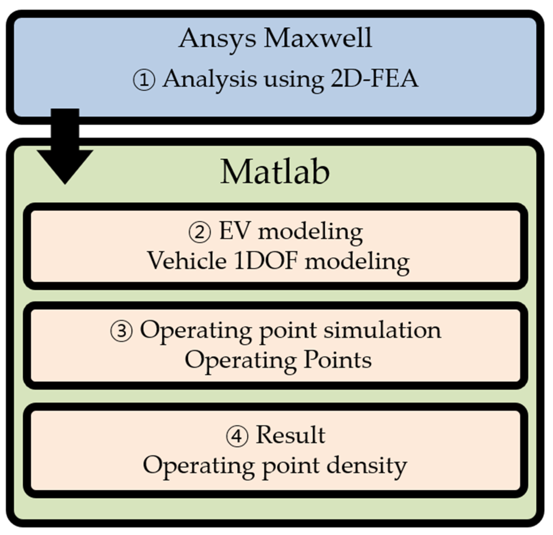
The process of the EV simulation is shown in Figure 2. The torque characteristics of the initial IPMSM motor model were analyzed using finite element analysis (FEA) performed with Ansys Maxwell. Subsequently, MATLAB 2024 was used to model the EV, and simulations were performed based on the selected driving cycle. The motor’s operating points derived from the simulation results were analyzed to choose the main operating points.

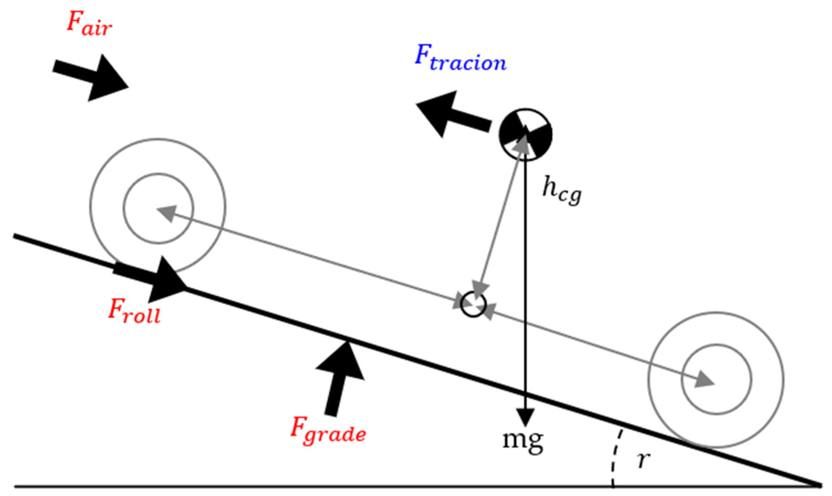
The EV modeling was conducted using MATLAB 2024 through a one-degree-of-freedom (1DOF) vehicle model. The 1DOF model represents the longitudinal motion of a vehicle with a single degree of freedom, considering only forward and backward movements. This allows the analysis of the vehicle’s longitudinal dynamics, as shown in Figure 3, and the calculation of the torque required by the motor during vehicle operation, as expressed in Equation (1). In Figure 3, the red text represents the resistance components acting against the vehicle’s motion, while the blue text indicates the traction force that propels the vehicle forward. Here, ${\mathrm{F}}_{\mathrm{t}\mathrm{r}\mathrm{a}\mathrm{c}\mathrm{t}\mathrm{i}\mathrm{o}\mathrm{n}}$ is the Traction force, ${\mathrm{F}}_{\mathrm{a}\mathrm{i}\mathrm{r}}$ is the air resistance, ${\mathrm{F}}_{\mathrm{g}\mathrm{r}\mathrm{a}\mathrm{d}\mathrm{e}}$ is the grade resistance and ${\mathrm{F}}_{\mathrm{R}\mathrm{o}\mathrm{l}\mathrm{l}}$ is the rolling resistance. In Equation (1), T represents the motor torque, $r$ denotes the wheel radius, $\eta$ is the gear efficiency, $G$ is the gear ratio, $M$ is the vehicle mass, $a$ is the vehicle acceleration, and $\mathsf{\rho }$ is the air density. Parameter $C_d$ is the drag coefficient, $A_f$ is the vehicle’s frontal area, $V$ is the vehicle speed, $f_r$ is the rolling resistance coefficient, $L$ is the wheelbase, $h_{cg}$ is the height of the center of gravity, $g$ is the gravitational acceleration, and $\gamma$ is the road gradient angle.

$$T={\displaystyle \frac{r}{\eta G}}(Ma+{\displaystyle \frac{1}{2}}\mathsf{\rho }{C}_d{A}_f{V}^2+f_r{\displaystyle \frac{L}{h_{cg}}}\mathrm{M}gcos\gamma +{\displaystyle \frac{L}{h_{cg}}}Mgsin\gamma )$$

(1)

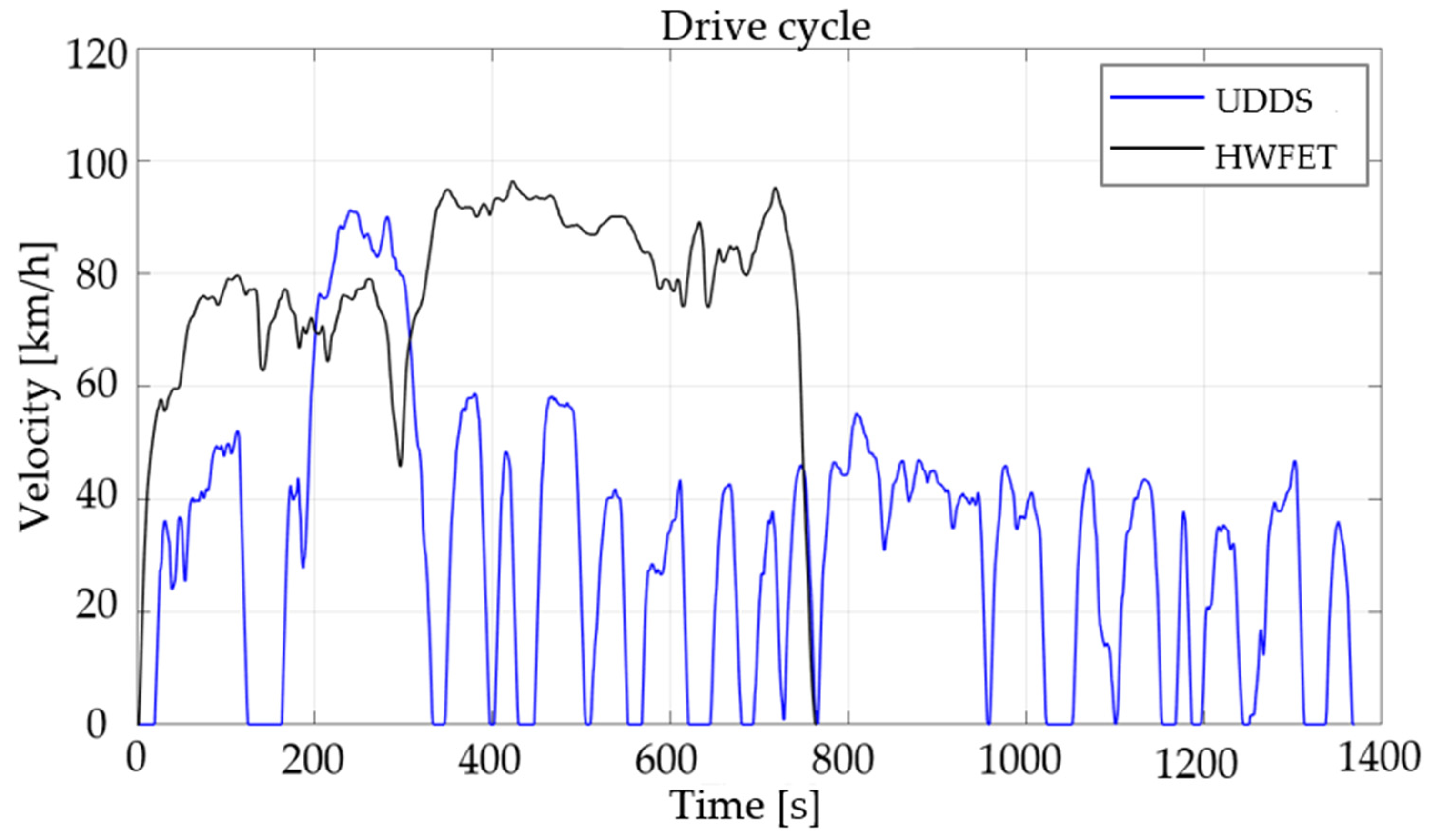
Previous optimal design studies using driving cycles have predominantly employed a single urban driving cycle to conduct simulations and determine the motor’s main operating points. In the EV driving range certification tests conducted by the Ministry of Environment in Korea, the Urban Dynamometer Driving Schedule (UDDS), which is an urban driving cycle involving frequent stops and accelerations over short distances, and the Highway Fuel Economy Driving Schedule (HWFET), a highway driving cycle involving relatively constant speeds at higher velocities, are used for the multi-cycle test (MCT); therefore, in this study, simulations were conducted using two driving cycles, UDDS and HWFET, based on the MCT test, as shown in Figure 4.

2.3. Operating Point Analysis

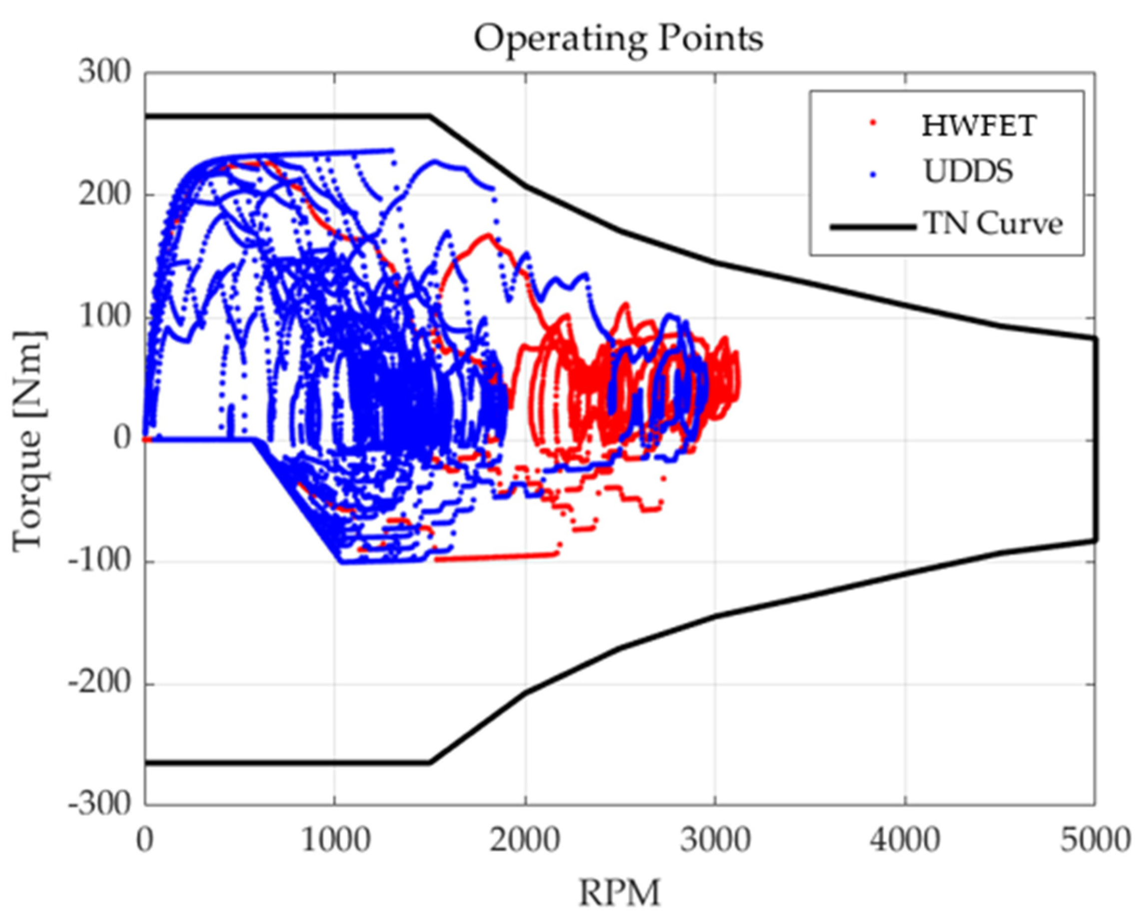
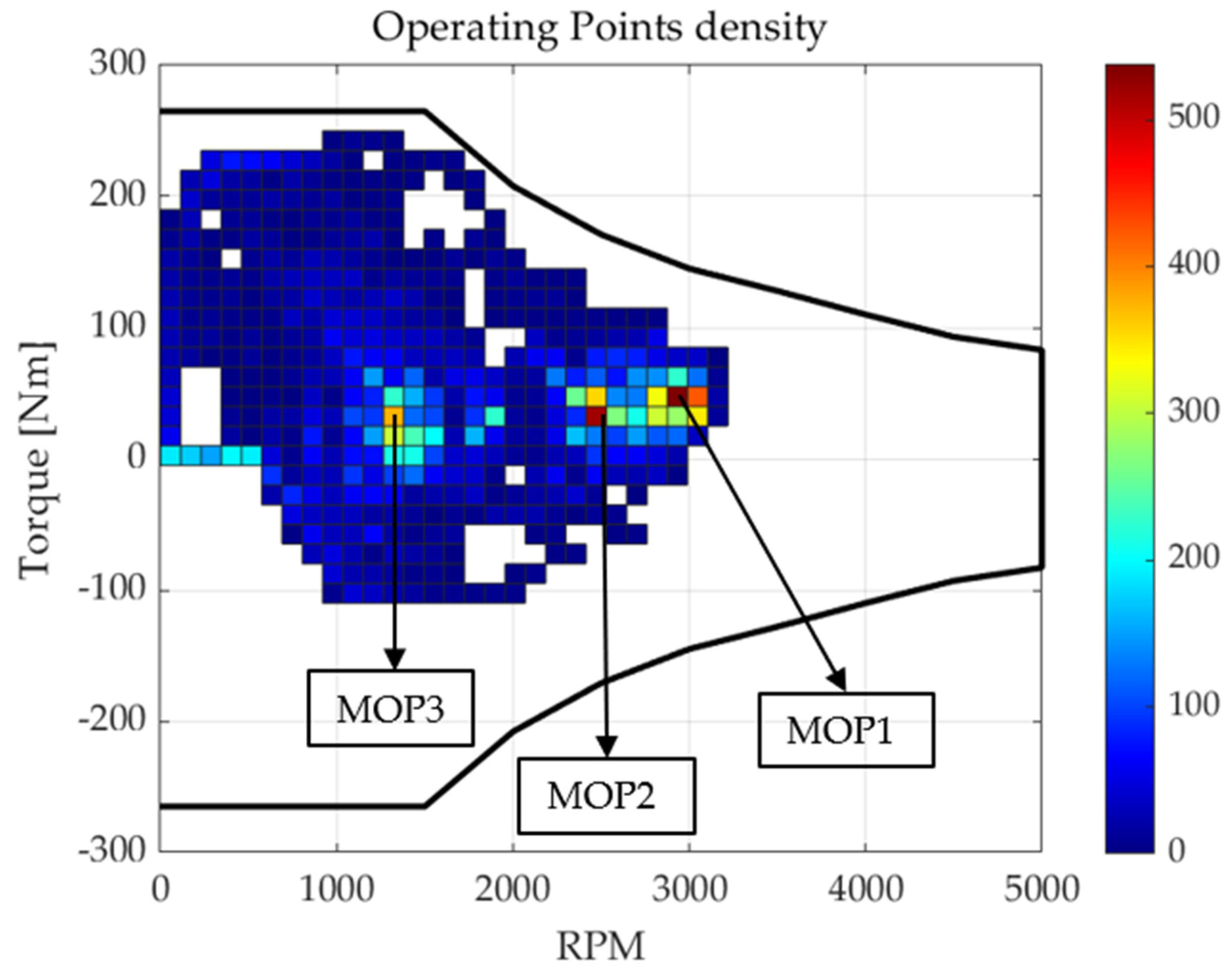
The motor’s operating points based on the driving cycles were derived from the simulation results, as shown in Figure 5. The three main operating points (MOPs) were determined by analyzing their density, as shown in Figure 6. MOP1 was within the range of 40 to 55 Nm and 2900 to 3000 rpm, MOP2 was within the range of 25 to 40 Nm and 2400 to 2500 rpm, and MOP3 was within the range of 25 to 40 Nm and 1265 to 1380 rpm. Out of 23,823 operating points, 537 points (2.25%) were in the MOP1 range, 519 points (2.17%) were in the MOP2 range, and 374 points (1.56%) were in the MOP3 range. Although the density of the operating points around the MOP1 range was also high, they were considered to overlap because they were within 100 rpm of the MOP1 range and were therefore excluded. The central point of each MOP area was selected as the final MOP point. The selected MOPs are presented in

Table 3. Selected main operating points.

Main Operating Points (MOP)	Speed (RPM)	Torque (Nm)	Percentage
MOP1	2900~3000 (2950)	40~55 (42.5)	537 (2.25%)
MOP2	2400~2500 (2450)	25~40 (32.5)	519 (2.17%)
MOT3	1265~1380 (1320)	25~40 (32.5)	374 (1.56%)

, with each MOP range followed by its central point indicated in parentheses.

3. Optimal Design

3.1. Design Problem Formulation

In this study, three main operating points were selected for efficient motor optimization, and the optimal design was achieved by combining the metamodels with optimization algorithms, as shown in Figure 7.

The optimization software PIAnO 2024 was employed, and the objective function was set to maximize the efficiency at the main operating points, as shown in Equation (2). The weights for each point were determined based on the density of the operating points, ensuring that their sum was equal to 1. Here, ${\mathit{\eta }}_{\mathit{i}}$ represents the efficiency of the main operating points and ${\mathit{w}}_{\mathit{i}}$ represents the weights of the main operating points. $T_{\mathit{Max}\_BaseRPM}$ is the maximum torque at the rated speed of 1575 rpm, and $T_{Max\_maxRPM}$ is the maximum torque at the maximum speed of 5000 rpm, set to 251 Nm and 80 Nm, respectively, to maintain an output of 40 kW and to maintain the values of the initial model. $T_{ripple}$ is the torque ripple at the rated speed, which was set to be below the allowable level of 10%, and, ${THD}_{Back-EMF}$ is the THD of the back electromotive force, which was set not to exceed the value of the initial model.

Additionally, $V_{line-to-line}$ is the line-to-line voltage and was constrained to 380 V to ensure it did not exceed the battery voltage, thereby formulating the design problem. During the DOE process, the input current beta angle at the rated speed was fixed, and at the maximum speed, the beta angle was set according to the voltage limit; therefore, $V_{line-to-line}$ represents the line-to-line voltage at the rated speed.

$$\begin{array}{cc}\mathrm{t}\mathrm{o} \mathrm{m}\mathrm{a}\mathrm{x}\mathrm{i}\mathrm{m}\mathrm{i}\mathrm{z}\mathrm{e}\hfill & {\sum }_{i=1}^3{\eta }_i{w}_i=({\eta }_1{w}_1+{\eta }_2{w}_2+{\eta }_3{w}_3)\hfill \\ \mathrm{s}\mathrm{u}\mathrm{b}\mathrm{j}\mathrm{e}\mathrm{c}\mathrm{t} \mathrm{t}\mathrm{o}\hfill & T_{Max\_BaseRPM}\ge 251 \mathrm{N}\mathrm{m}\hfill \\ \hfill & T_{Max\_maxRPM}\ge 80 \mathrm{N}\mathrm{m}\hfill \\ \hfill & T_{ripple}\le 10\%\hfill \\ \hfill & {THD}_{Back-EMF}\le 8\%\hfill \\ \hfill & V_{line-to-line}\le 380 \mathrm{V}\hfill \end{array}$$

(2)

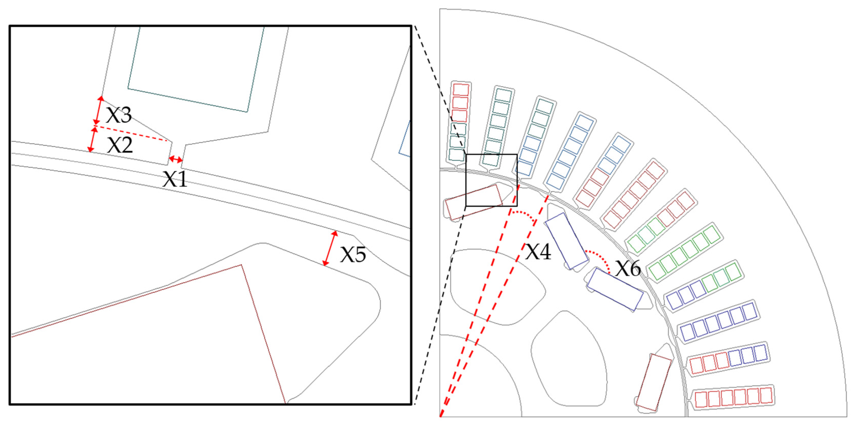
Six design variables were selected based on the objectives and constraints, and their minimum and maximum ranges are presented in

Table 4. Range of variables.

Design Variables	Unit	Lower	Initial	Upper
X1 (Slot open)	mm	0.4	0.41	3.6
X2 (Shoe thickness)	mm	0.5	0.7	2
X3 (Shoe angle)	mm	0	0.85	2
X4 (Notch angle)	°	5.2	7.21	7.5
X5 (Rib thickness)	mm	0.9	0.9	2
X6 (Magnet angle)	°	135	145	155

. The configurations of the design variables are shown in Figure 8. X1 represents the open slot, with a lower limit of 0.4 mm, which is the minimum thickness required for mold production considering manufacturability, and an upper limit of 3.6 mm, which is smaller than the winding size to ensure that the winding does not protrude. X2 denotes the Shoe thickness, with a lower limit of 0.5 mm, considering the minimum thickness of 5 mm required for mold production of the shoe area, and an upper limit of 2 mm to ensure that the flux density of the back yoke does not exceed 1.8 T, considering the armature reaction [23]. Considering the armature reaction, X3 represents the Shoe angle, with a lower limit of 0 mm and an upper limit of 2 mm. X4 is the Notch angle, with a lower limit of 5.2° and an upper limit of 7.5°, ensuring that the surrounding thickness is at least 0.5 mm for die manufacturability. X5 denotes the Rib thickness, with a lower limit of 0.9 mm and an upper limit of 2 mm, ensuring that the surrounding area maintains a thickness of 0.5 mm for mold production. X6 represents the Magnet angle, where holes are placed in rotor areas with low flux density for motor weight reduction, with the range set to ensure that the flux density around these holes remains below the original value of 0.2 T.

3.2. Sensitivity Analysis

A sensitivity analysis was performed to select the design variables significantly affecting the objective and constraint functions. The number of experimental points for the analysis was determined using the Orthogonal Array (OA) method, a DOE technique designed to reduce the number of experimental points compared with the Full-Factorial Design (FFD) method. The experimental points were selected according to Equation (3) [24].

nEXP ≥ 1.5 × (nDV + 1) (nDV + 2)/2,

(3)

where nEXP is the number of experimental points, and nDV is the number of design variables. According to Equation (3), the experimental points should be at least 42. To consider the nonlinear changes in the output and characteristics of the OA, each design variable was set at three levels, and 45 experimental points closest to the calculated number of experimental points in the OA table were selected. FEA was performed, and based on the results, an Analysis of Variance (ANOVA) was conducted to calculate the probability value (p-value) at a significance level of 0.05. This method was used to compare means between different groups to determine whether differences between groups were statistically significant. The results are presented in

Table 5. Analysis results of the p-value.

Items	X1	X2	X3	X4	X5	X6
MOP1	0	0.485	0.185	0.636	0	0.975
MOP2	0.028	0.02	0.001	0.828	0	0.18
MOP3	0.016	0	0	0.927	0	0.362
${THD}_{Back-EMF}$	0	0.053	0.062	0.04	0.001	0
$T_{\mathit{Max}\_BaseRPM}$	0	0.405	0.05	0.129	0	0.132
$T_{Max\_maxRPM}$	0	0	0.092	0.022	0	0.474
$V_{line-to-line}$	0	0	0	0.006	0.006	0.003
$T_{ripple}$	0.039	0.967	0.849	0.89	0.043	0.219

, where values below the significance level of 0.05 are shaded [25,26]. A p-value less than 0.05 indicates that the factor has a statistically significant impact on the results and affects the objectives.

Although the X4_Notch angle is significant based on the p-value, its impact is lower than that of the other variables when the proportions are compared according to the Sum-of-Squares (SS) values, representing the magnitude of variation for each design variable; therefore, considering the number of experimental points and the accuracy of the metamodel, the X4 notch angle was excluded as a design variable. The SS values are summarized in

Table 6. Analysis results of SS.

Items	X1	X2	X3	X4	X5	X6
MOP1	52.4	1.26	3.18	0.84	42.31	0.04
MOP2	7.63	10.45	21.42	0.37	56.52	3.6
MOP3	7.39	22.89	34.96	0.12	33.06	1.58
${THD}_{Back-EMF}$	58.57	2.02	1.86	2.19	12.52	22.84
$T_{\mathit{Max}\_BaseRPM}$	11.36	1	3.5	2.39	79.41	2.34
$T_{Max\_maxRPM}$	72.31	9.74	2.61	4.44	10.12	0.79
$V_{line-to-line}$	50.02	20.98	17.54	3.69	3.27	4.5
$T_{ripple}$	41.6	0.36	1.84	1.26	37.87	17.06

. The five design variables X1, X2, X3, X5, and X6 significantly impact the objective and constraint functions; thus, the optimal design was determined using the selected design variables.

3.3. Metamodeling

The optimal metamodeling technique depends on the distribution of the test values; therefore, to develop the optimal metamodel for the objective and constraint functions, 11 metamodels were compared and selected based on the Root Mean Square Error (RMSE) test values [27]. The metamodeling techniques employed include the Ensemble of Decision Trees (EDT), which combines multiple decision trees to enhance the robustness and accuracy of the predictive model, effectively modeling nonlinear relationships [28]; Kriging (KRG), which approximates complex relationships between design variables and objectives based on spatial correlations and contributes to improving reliability by enabling uncertainty evaluation [29]; Multi-layer Perceptron (MLP), which is a type of artificial neural network with one or more hidden layers, that learn nonlinear relationships between input and output variables and effectively solves complex design problems [30]; and Polynomial Regression (PRG) techniques, which model the relationship between one or more independent variables and a dependent variable using polynomials. PRG (Polynomial Regression) techniques approximate the relationship between design variables and objectives and are divided into various sub-models depending on the complexity of the problem and the degree of interaction between design variables. PRG Linear Model (LR) expresses simple linear relationships, while PRG Full Quadratic Model (FQ) incorporates second-order polynomials and interaction terms to model more complex relationships. PRG Simple Quadratic Model (SQ) and Simple Cubic Model (SC) handle second and third-order polynomials, respectively, to address nonlinear characteristics. Furthermore, PRG Forward Step (FG) and Backward Step (BS) utilize variable selection algorithms to adjust model complexity and improve efficiency [31]. Radial Basis Function (RBF) techniques, which transform the input space into a high-dimensional feature space using functions that vary based on the distance from the center, are also employed. RBF techniques use functions that vary with the distance from a center point to model nonlinear relationships between design variables and objectives effectively. These techniques are further divided into RBF Interpolation (Int) and RBF Regression (Reg), depending on the characteristics of these data. RBF Interpolation (Int) generates functions that precisely pass through the given data points and are suitable for cases where exact reproduction of these data is required. Conversely, RBF Regression (Reg) employs approximation methods to provide generalized results even for noisy datasets, allowing for a smoother representation of the relationships between design variables and objectives [32]. An RMSE test value closer to zero indicates a smaller prediction error between the metamodel and the actual FEA experimental point values. To apply the RMSE test, the number of experimental points was determined according to Equation (4).

nEXP > Min [(nDV + 1) (nDV + 2)/2, 10 × nDV] + 5 × nDV

(4)

nTS = min [0.1 × nEXP, 10 × nDV]

(5)

where nTS denotes the number of test points used to evaluate the metamodel performance. According to Equation (5), the experimental points must exceed 46; therefore, 54 points were selected from the OA table that satisfied the condition of being 46 or more, and the RMSE test was conducted using six test points. The results are presented in

Table 7. RMSE test results.

Items	EDT	KRG	MLP	PRG (BS)	PRG (FS)	PRG (FQ)	PRG (LR)	PRG (SC)	PRG (SQ)	RBF (Int)	RBF (Reg)
MOP1	0.0155	0.0129	0.0559	18.9496	0.0471	0.0479	0.0675	0.0479	0.0772	0.0608	0.0519
MOP2	0.0608	0.0287	0.153	0.0361	0.0361	0.0436	0.0714	0.0436	0.0889	0.0648	0.0708
MOP3	0.0549	0.0335	0.0643	0.0428	0.0418	0.048	0.0682	0.048	0.0775	0.0596	0.0418
${THD}_{Back-EMF}$	0.2932	0.3955	0.5494	0.837	0.7324	1.075	1.8461	1.075	1.5921	0.6765	1.0536
$T_{\mathit{Max}\_BaseRPM}$	3.4306	3.3266	1.9608	2.3048	2.3048	1.9746	5.1139	1.9746	2.877	1.0895	2.2645
$T_{Max\_maxRPM}$	6.1921	3.3484	3.9955	9.6987	8.932	9.73	8.5624	9.73	9.3322	15.3482	9.0585
$V_{line-to-line}$	4.8343	4.9383	3.0527	6.1588	5.5731	5.0595	9.315	5.0595	6.9336	3.6986	3.4286
$T_{ripple}$	0.0202	0.0275	0.0168	0.0273	0.0324	0.0243	0.0474	0.0243	0.0414	0.0268	0.0246

.

KRG was selected as the most suitable metamodeling technique for MOP1, MOP2, MOP3, and $T_{Max\_maxRPM}$, while EDT was chosen for ${THD}_{Back-EMF}$, RBF for $T_{\mathit{Max}\_BaseRPM}$ RBF (Int.), and MLP for $V_{line-to-line}$, $T_{ripple}$.

3.4. Optimal Design Results

The optimal metamodels for the selected objective and constraint functions were combined with optimal design algorithms to derive the optimal points. Micro Genetic Algorithm (MGA), a type of Evolutionary Algorithm (EA), employs a small population size to achieve fast exploration and convergence [33]. Similarly, the Covariance Matrix Adaptation-Evolutionary Strategy (CMA-ES), another type of EA, improves the convergence speed using a multivariate normal distribution [34]. Progressive Approximate Discrete Optimization (PADO) addresses discrete optimization problems by progressively refining approximate solutions [35], and the Hybrid Metaheuristic Algorithm (HMA) is a global optimization algorithm [36]. The optimal design was determined using four algorithms, and the results are summarized in

Table 8. Optimal design results using the optimization algorithm.

Items		Unit	Initial	MGA	CMA-ES	PADO	HMA
Objective Function	MOP3	%	95.85	95.94	95.93	95.99	95.93
	MOP2	%	95.99	96.46	96.03	96.06	96.03
	MOP1	%	96.45	96.56	96.52	96.55	96.52
Constraints	${THD}_{Back-EMF}$	%	8.01	6.88	7.4	6.89	7.4
	$T_{\mathit{Max}\_BaseRPM}$	Nm	250.6	247.7	248.3	247	248.5
	$T_{Max\_maxRPM}$	Nm	76.48	83.17	90.49	83.19	83.79
	$V_{line-to-line}$	V	362.4	360	358.95	365.1	363.5
	$T_{ripple}$	V	8.74	8.83	9.21	6.12	8.92

.

When employing the MGA algorithm for optimal design, the efficiency at the main operating points, which was the objective function, exhibited the most significant increase and was thus selected as the optimal point. FEA was performed on the optimal point to verify the accuracy of the metamodel predictions and the validity of the optimal design.

Table 9. Optimal design results using the MGA algorithm.

Items		Unit	Initial	Optimal (Metamodel)	Optimal (FEA)
Design Variables	X1	mm	0.41	1.71
	X2	mm	0.7	0.54
	X3	mm	0.85	1.5
	X4	mm	0.9	1.24
	X5	°	145	140
Objective Function	MOP1	%	95.73	96.52	96.56
	MOP2	%	95.99	96.32	96.46
	MOP3	%	95.85	95.86	95.94
Constraints	${THD}_{Back-EMF}$	%	8.01	6.49	6.88
	$T_{\mathit{Max}\_BaseRPM}$	Nm	250.55	248.82	247.73
	$T_{Max\_maxRPM}$	Nm	76.48	83.16	83.17
	$V_{line-to-line}$	V	362.37	357.93	360
	$T_{ripple}$	%	8.74	8.88	8.93

compares the results obtained by the metamodel and FEA, as well as those of the initial and optimal models.

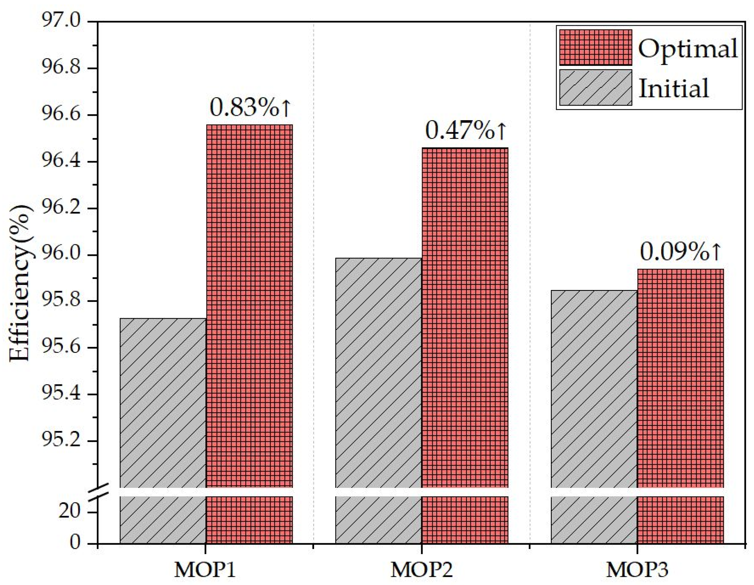
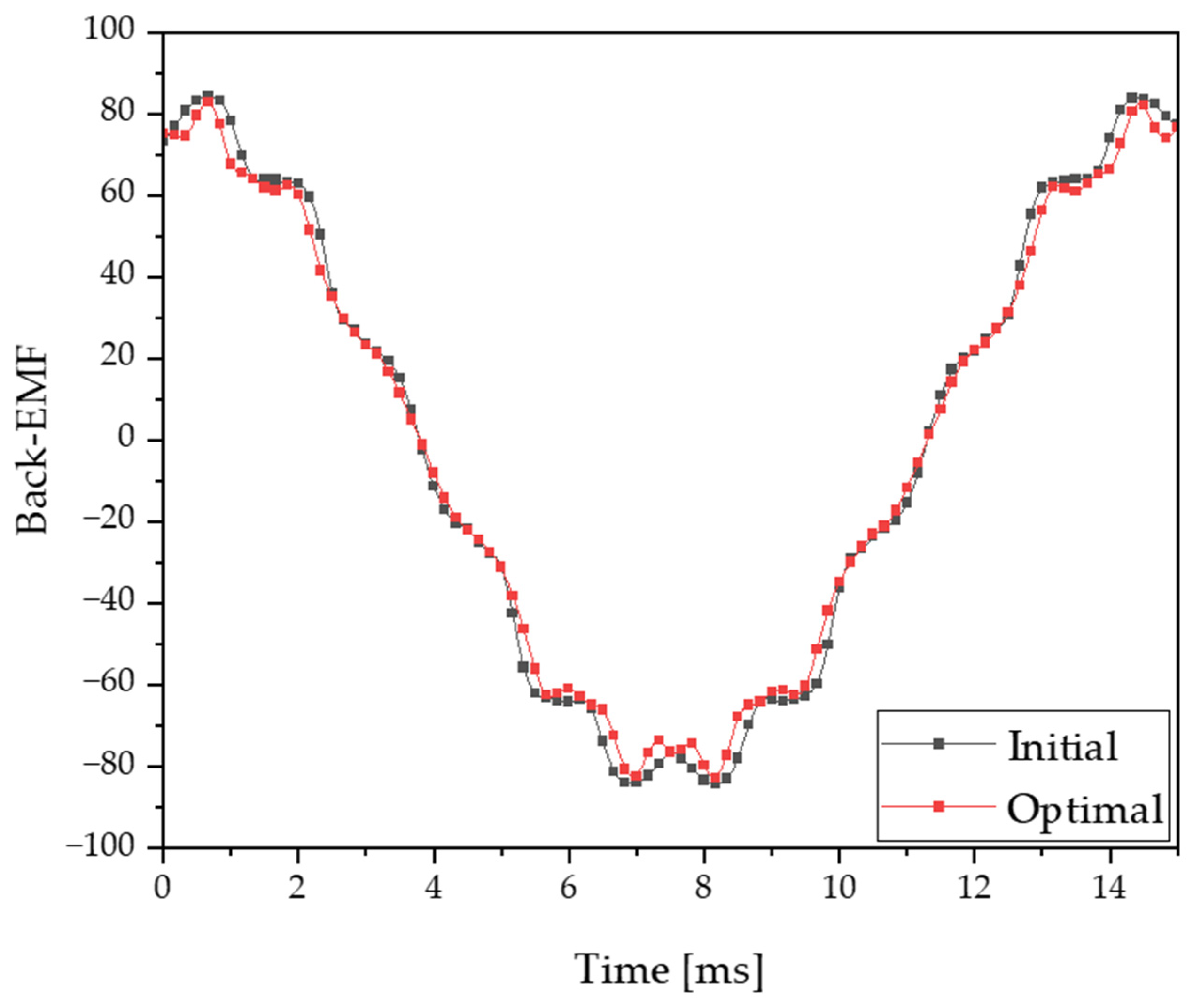
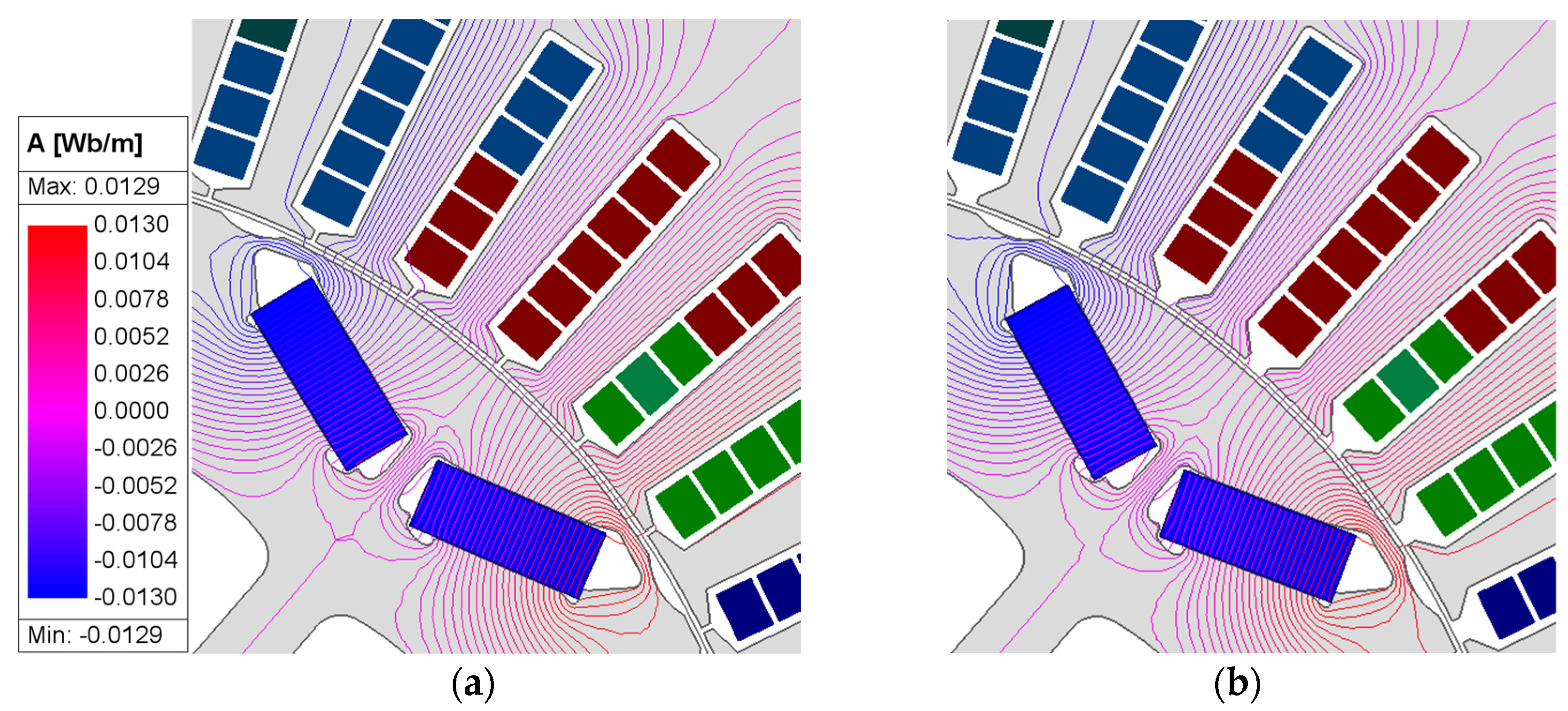
As a result of the optimal design, the efficiency at the main operating points increased by 1.4% compared with the initial model, with an increase of 0.83% at MOP1, 0.47% at MOP2, and 0.09% at MOP3, as shown in Figure 9. ${THD}_{Back-EMF}$ decreased by 1.13%, and Figure 10 compares the back electromotive force waveforms of the initial and optimal models. $T_{Max\_maxRPM} \mathrm{i}\mathrm{n}\mathrm{c}\mathrm{r}\mathrm{e}\mathrm{a}\mathrm{s}\mathrm{e}\mathrm{d} \mathrm{b}\mathrm{y} 6.69 \mathrm{N}\mathrm{m}; \mathrm{h}\mathrm{o}\mathrm{w}\mathrm{e}\mathrm{v}\mathrm{e}\mathrm{r}, T_{\mathit{Max}\_BaseRPM}$ did not meet the constraint of 251 Nm. This is because the allowable tolerance limit (Violated Constraint Limit) in the optimization software PIAnO 2024 was set to 1%. An excessively low or absent allowable tolerance limit can lead to a lengthy, nonconvergent optimization process, resulting in sub-optimal solutions. $V_{line-to-line}$ and $T_{ripple}$ satisfied the constraints; therefore, the model derived by combining the metamodel and MGA algorithm was determined to be the optimal model, and its geometry is shown in Figure 11.

4. Conclusions

This study optimizes the efficiency of an EV IPMSM motor featuring hairpin windings by selecting the main operating points based on a driving cycle. The selection process employed MATLAB 2024 to analyze the density of operating points, enabling the identification of effective optimal design points for an EV drive motor while considering the loss values that fluctuate between low- and high-speed operating regions, particularly the increasing AC copper loss at higher operating speeds. To enhance the validity of the operating point selection, EV simulations considered all driving cycles of the MCT method used for driving range measurements in Korea. The design problem was formulated by considering the critical motor parameters, specifically, the torque ripple and the THD of the back-EMF. 11 metamodels were used to determine the optimal metamodel, which varied according to the distribution of experimental points based on the design problem, output, and constraints. The RMSE test was used to select the metamodel with the optimal predictive value for the objective and constraint functions, and the optimal design was determined using four optimization algorithms. The optimal point combined with the MGA algorithm was verified to validate the optimal design via FEA. The efficiency of the selected optimal model improved by 0.83% at MOP1, 0.47% at MOP2, and 0.09% at MOP3, representing a total improvement of 1.4% compared with the initial model. Additionally, the improved efficiency contributed to a 1.13% reduction in the THD of the back-EMF, indicating smoother flux flow. This research confirms that a highly accurate metamodel and valid selection of the main operating points enable an efficient optimal design for an EV drive motor.

References

1. Abas, A.E.P.; Yong, J.; Mahlia, T.M.I.; Hannan, M.A. Techno-Economic Analysis and Environmental Impact of Electric Vehicle. IEEE Access 2019, 7, 98565–98578. [Google Scholar] [CrossRef]
2. Heffner, R.R.; Kurani, K.S.; Turrentine, T.S. Symbolism in California’s early market for hybrid electric vehicles. Transp. Res. Part D Transp. Environ. 2007, 12, 396–413. [Google Scholar] [CrossRef]
3. Karvonen, M.; Klemola, K.; Ranaei, S.; Kässi, T. Predicting the technological paths in automotive industry and the environmental impacts of electrification of automotive industry in selected OECD countries. In Proceedings of the 2015 Portland International Conference on Management of Engineering and Technology (PICMET), Portland, OR, USA, 2–6 August 2015; pp. 1247–1259. [Google Scholar] [CrossRef]
4. Bilgin, B.; Magne, P.; Malysz, P.; Yang, Y.; Pantelic, V.; Preindl, M.; Korobkine, A.; Jiang, W.; Lawford, M.; Emadi, A. Making the Case for Electrified Transportation. IEEE Trans. Transp. Electrif. 2015, 1, 4–17. [Google Scholar] [CrossRef]
5. Bianchi, N.; Bolognani, S. Interior PM synchronous motor for high performance applications. In Proceedings of the Power Conversion Conference-Osaka 2002 (Cat. No.02TH8579), Osaka, Japan, 2–5 April 2002; Volume 1, pp. 148–153. [Google Scholar] [CrossRef]
6. Yang, Y.; Castano, S.M.; Yang, R.; Kasprzak, M.; Bilgin, B.; Sathyan, A.; Dadkhah, H.; Emadi, A. Design and Comparison of Interior Permanent Magnet Motor Topologies for Traction Applications. IEEE Trans. Transp. Electrif. 2017, 3, 86–97. [Google Scholar] [CrossRef]
7. Popescu, M.; Goss, J.; Staton, D.A.; Hawkins, D.; Chong, Y.C.; Boglietti, A. Electrical Vehicles—Practical Solutions for Power Traction Motor Systems. IEEE Trans. Ind. Appl. 2018, 54, 2751–2762. [Google Scholar] [CrossRef]
8. Park, H.-J.; Lim, M.-S. Design of High Power Density and High Efficiency Wound-Field Synchronous Motor for Electric Vehicle Traction. IEEE Access 2019, 7, 46677–46685. [Google Scholar] [CrossRef]
9. Kim, C.-M.; Kim, K.-C. A Study on the Winding Method and Skew Effect Electromagnetic Field Characteristics of Hairpin Winding for High Power Density Motor Design. J. Korea Contents Assoc. 2023, 23, 17–25. [Google Scholar] [CrossRef]
10. Shams Ghahfarokhi, P.; Podgornovs, A.; Cardoso, A.J.M.; Kallaste, A.; Belahcen, A.; Vaimann, T. Hairpin Windings for Electric Vehicle Motors: Modeling and Investigation of AC Loss-Mitigating Approaches. Machines 2022, 10, 1029. [Google Scholar] [CrossRef]
11. Jun, S.-B.; Kim, D.-W.; Kim, J.-S.; Ko, Y.-Y.; Kim, Y.-J.; Jung, S.-Y. Comparison on the Charateristics of AC Copper Loss on IPMSM for EV Traction according to the Number of Conductors. J. Inst. Inf. Telecommun. Facil. Eng. 2019, 15, 6–11. [Google Scholar]
12. Ju, X.; Cheng, Y.; Du, B.; Yang, M.; Yang, D.; Cui, S. AC Loss Analysis and Measurement of a Hybrid Transposed Hairpin Winding for EV Traction Machines. IEEE Trans. Ind. Electron. 2023, 70, 3525–3536. [Google Scholar] [CrossRef]
13. Chin, J.-W.; Cha, K.-S.; Park, M.-R.; Park, S.-H.; Lee, E.-C.; Lim, M.-S. High Efficiency PMSM With High Slot Fill Factor Coil for Heavy-Duty EV Traction Considering AC Resistance. IEEE Trans. Energy Convers. 2021, 36, 883–894. [Google Scholar] [CrossRef]
14. Hebala, A.; Nuzzo, S.; Connor, P.H.; Volpe, G.; Gerada, C.; Galea, M. Mitigation of AC Winding Losses for Aircraft Propulsion Motors. In Proceedings of the IECON 2022—48th Annual Conference of the IEEE Industrial Electronics Society, Brussels, Belgium, 17–20 October 2022; pp. 1–6. [Google Scholar] [CrossRef]
15. Carraro, E.; Morandin, M.; Bianchi, N. Traction PMASR Motor Optimization According to a Given Driving Cycle. IEEE Trans. Ind. Appl. 2016, 52, 209–216. [Google Scholar] [CrossRef]
16. Salameh, M.; Brown, I.P.; Krishnamurthy, M. Fundamental Evaluation of Data Clustering Approaches for Driving Cycle-Based Machine Design Optimization. IEEE Trans. Transp. Electrif. 2019, 5, 1395–1405. [Google Scholar] [CrossRef]
17. Chen, L.; Wang, J.; Lazari, P.; Chen, X. Optimizations of a permanent magnet machine targeting different driving cycles for electric vehicles. In Proceedings of the 2013 International Electric Machines & Drives Conference, Chicago, IL, USA, 12–15 May 2013; pp. 855–862. [Google Scholar] [CrossRef]
18. Ahn, K.; Bayrak, A.E.; Papalambros, P.Y. Electric Vehicle Design Optimization: Integration of a High-Fidelity Interior-Permanent-Magnet Motor Model. IEEE Trans. Veh. Technol. 2015, 64, 3870–3877. [Google Scholar] [CrossRef]
19. Yoon, K.-Y.; Hwang, K.-Y. Optimal Design of Spoke-Type IPM Motor Allowing Irreversible Demagnetization to Minimize PM Weight. IEEE Access 2021, 9, 65721–65729. [Google Scholar] [CrossRef]
20. Li, Y.; Song, B.; Mao, Z.; Tian, W. Analysis and Optimization of the Electromagnetic Performance of a Novel Stator Modular Ring Drive Thruster Motor. Energies 2018, 11, 1598. [Google Scholar] [CrossRef]
21. Ahn, J.-M.; Baek, M.-K.; Park, S.-H.; Lim, D.-K. Optimal Design of IPMSM for EV Using Subdivided Kriging Multi-Objective Optimization. Processes 2021, 9, 1490. [Google Scholar] [CrossRef]
22. Cho, S.-K.; Jung, K.-H.; Choi, J.-Y. Design Optimization of Interior Permanent Magnet Synchronous Motor for Electric Compressors of Air-Conditioning Systems Mounted on EVs and HEVs. IEEE Trans. Magn. 2018, 54, 8204705. [Google Scholar] [CrossRef]
23. Bae, J.-N. Permanent Magnet Synchronous Machine Design Through an Automatic Selection of the Specific Loadings. Doctoral Dissertation, Hanyang University, Seoul, Republic of Korea, 2010. [Google Scholar]
24. Kacker, R.N.; Lagergren, E.S.; Filliben, J.J. Taguchi’s Orthogonal Arrays Are Classical Designs of Experiments. J. Res. Natl. Inst. Stand. Technol. 1991, 96, 577–591. [Google Scholar] [CrossRef]
25. Brenneman, M.T.; Morton, Y.T.; Zhou, Q. GPS Multipath Detection with ANOVA for Adaptive Arrays. IEEE Trans. Aerosp. Electron. Syst. 2010, 46, 1171–1184. [Google Scholar] [CrossRef]
26. Patil, N.S.; Yaligar, M.F. Analysis of linear relation between P-value and co relational value using R programming. In Proceedings of the 2017 International Conference on Advances in Computing, Communications and Informatics (ICACCI), Udupi, India, 13–16 September 2017; pp. 983–987. [Google Scholar] [CrossRef]
27. Hodson, T.O. Root-mean-square error (RMSE) or mean absolute error (MAE): When to use them or not. Geosci. Model Dev. 2022, 15, 5481–5487. [Google Scholar] [CrossRef]
28. Mienye, D.; Jere, N. A Survey of Decision Trees: Concepts, Algorithms, and Applications. IEEE Access 2024, 12, 86716–86727. [Google Scholar] [CrossRef]
29. Lebensztajn, L.; Marretto, C.A.R.; Costa, M.C.; Coulomb, J.L. Kriging: A useful tool for electromagnetic device optimization. IEEE Trans. Magn. 2004, 40, 1196–1199. [Google Scholar] [CrossRef]
30. Al Bataineh, A.; Kaur, D.; Jalali, S.M.J. Multi-Layer Perceptron Training Optimization Using Nature Inspired Computing. IEEE Access 2022, 10, 36963–36977. [Google Scholar] [CrossRef]
31. Hakim, M.; Choukri, S. Polynomial Metamodelling of Computer Simulation for UAV Design. In Proceedings of the 2024 4th International Conference on Innovative Research in Applied Science, Engineering and Technology (IRASET), FEZ, Morocco, 16–17 May 2024; pp. 1–5. [Google Scholar] [CrossRef]
32. Lei, Y.; Ding, L.; Zhang, W. Generalization Performance of Radial Basis Function Networks. IEEE Trans. Neural Netw. Learn. Syst. 2015, 26, 551–564. [Google Scholar] [CrossRef]
33. Chakravarty, S.; Mittra, R.; Williams, N.R. Application of a microgenetic algorithm (MGA) to the design of broadband microwave absorbers using multiple frequency selective surface screens buried in dielectrics. IEEE Trans. Antennas Propag. 2002, 50, 284–296. [Google Scholar] [CrossRef]
34. Akimoto, Y.; Hansen, N. Diagonal Acceleration for Covariance Matrix Adaptation Evolution Strategies. Evol. Comput. 2020, 28, 405–435. [Google Scholar] [CrossRef]
35. Yahagi, H.; Shimizu, S.; Ogata, T.; Hara, T.; Ota, J. Simulation-Based Rule Generation Considering Readability. Int. Sch. Res. Not. 2015, 2015, 159289. [Google Scholar] [CrossRef]
36. Lü, Z.; Glover, F.; Hao, J.-K. A hybrid metaheuristic approach to solving the UBQP problem. Eur. J. Oper. Res. 2010, 207, 1254–1262. [Google Scholar] [CrossRef]
Figure 1. Initial model.
Applsci 15 00368 g001
Figure 2. Main operating point selection process.
Applsci 15 00368 g002
Figure 3. Vehicle dynamics.
Applsci 15 00368 g003
Figure 4. UDDS and HWFET driving cycles.
Applsci 15 00368 g004
Figure 5. Operating points EV simulation.
Applsci 15 00368 g005
Figure 6. Operating point density.
Applsci 15 00368 g006
Figure 7. Optimal design process.
Applsci 15 00368 g007
Figure 8. Shape of design variables.
Applsci 15 00368 g008
Figure 9. Efficiency in main operating points.
Applsci 15 00368 g009
Figure 10. Back-EMF waveforms.
Applsci 15 00368 g010
Figure 11. Magnetic flux lines (a) initial model (b) optimal model.
Applsci 15 00368 g011