Driver Clustering Based on Individual Curve Path Selection Preference

Abstract

The development of Advanced Driver Assistance Systems (ADASs) has reached a stage where, in addition to the traditional challenges of path planning and control, there is an increasing focus on the behavior of these systems. Assistance functions shall be personalized to deliver a full user experience. Therefore, driver modeling is a key area of research for next-generation ADASs. One of the most common tasks in everyday driving is lane keeping. Drivers are assisted by lane-keeping systems to keep their vehicle in the center of the lane. However, human drivers often deviate from the center line. It has been shown that the driver’s choice to deviate from the center line can be modeled by a linear combination of preview curvature information. This model is called the Linear Driver Model. In this paper, we fit the LDM parameters to real driving data. The drivers are then clustered based on the individual parameters. It is shown that clusters are not only formed by the numerical similarity of the driver parameters, but the drivers in a cluster actually have similar behavior in terms of path selection. Finally, an Extended Kalman Filter (EKF) is proposed to learn the model parameters at run-time. Any new driver can be classified into one of the driver type groups. This information can be used to modify the behavior of the lane-keeping system to mimic human driving, resulting in a more personalized driving experience.

1. Introduction

The development of Advanced Driver Assistance Systems (ADASs) reached a maturity level where, besides technological challenges, the behavior of these systems is getting more and more focus. While automated driving functions can handle various driving tasks, their behavior is highly different from that of human drivers. One of the most controversial functions is the lane centering system (LCS). People often claim that LCS is annoying, and therefore, they switch it off. In many cases, car buyers refuse to purchase the newer generation of LCS. This hinders the widespread use of higher-level automated driving systems. Also, LCS is not only a comfort function, but it also aids drivers in emergency situations. The dislike of this system is therefore directly related to driving safety problems. By realizing the situation, car manufacturers decided to invest research effort in making lane centering systems more human-like, which eventually results in better acceptance of these systems. In order to achieve human-likeness, it is a common approach to observe people’s naturalistic driving and build models that can reproduce their behavior. It is observed that drivers do not always drive in the center of the lane [1,2]. Therefore, driver models in the field of path planning aim to plan the position offset of the vehicle to the centerline. The latest solutions in the field, such as the Generalized Regression Neural Network (GRNN) model [3], the Long-Short-Term-Memory (LSTM) model [4], or the Preview Horizon Trajectory Planning Model (PHTPM) [5], all use certain neural network structures. Even though these models are exceptionally accurate, they are difficult to use for driver clustering, as they have no model parameters. Further trajectory planning analysis work was conducted to distinguish drivers based on their risk-taking willingness [6]. Even though such papers give remarkable insight into driving behavior mechanisms, the modeling of the analyzed behavior is not straightforward. Other driver models from the vehicle control fields, such as the Pure-Pursuit algorithm [7], Model Predictive Control (MPC) models [8,9,10], or the compensatory driver model [11], describe the drivers’ control, and not their planning behavior, which is a much more limited view of the complete driving procedure. There are parametric driver models such as the Linear Driver Model (LDM) that give a simple but robust description of the drivers’ path planning behavior [12], and their parameters make it possible to directly quantify one’s path planning policy. After the selected driver model is trained, it can be used to reproduce the path selection of the driver. However, learning the behavior of all drivers individually would result in a theoretically infinite number of behavioral variations. This makes practical utilization difficult. Therefore, drivers are classified into behavioral groups. These are reference groups that must be created first. For that, unsupervised learning (i.e., clustering) is applied to the learned parameters of reference drivers. Then, the resulting driver groups are compared with judge their behavior. Such concepts are used in the literature. Driving styles are identified via clustering drivers based on their driving dynamics [13,14], their curve speed selection [15] or time-to-collision [13]. These papers use the k-means algorithm, on an average 25–30 test drivers, that are clustered to 3–4 groups (e.g., dynamic, normal and comfortable). However, these solutions use directly the measured driving quantities, and they do not use any higher-level driver models. Assuming the driving groups are created, the parameters of a new driver can be learned, and he can be classified into one of the groups. Practically, this happens in real time while the driver is driving. Therefore, the algorithm of parameter learning must be computationally efficient enough in order to implement it on an embedded control unit. In case of parametric models, parameter identification solutions, such as Kalman filters are often used [16,17]. These algorithms use very little memory while having relatively fast convergence. Moreover, if the driver behavior and hence their parameters are changed (e.g., due to influencing factors of exhaustiveness, traffic, mood … etc.) they can automatically adapt the parameters.

In this paper, we introduce a comprehensive solution for how lane centering systems can be made more human-like. We exploit existing components of the literature, from parametric driver model clustering to parameter identification techniques. To the best of our knowledge, there are no existing solutions in the literature that cover the entire driver modeling and clustering chain, including real-time parameter identification options. Also, using simple and robust driver modeling, applications with lower computational capacity—especially car manufacturers in the lower vehicle categories—are possible, enhancing the ADAS functionality in a wide range of vehicles. The main contributions are the following:

C1

We cluster drivers based on their curve path preferences, using the Linear Driver Model and its parameters, and in this way, behavioral differences are quantified. It is shown that the clusters are indeed different in their curve driving behavior. Two groups of dynamic and cautious drivers are created that are used as reference groups for the classification.

C2

An Extended Kalman Filter-based approach is proposed to learn the driver model parameters. It is proven that this solution is suitable for embedded applications as its computational needs are low, while its convergence to the real parameter values is fast. This way, a compact solution is introduced that can be directly used for the next generation of lane centering systems.

2. Methods and Materials

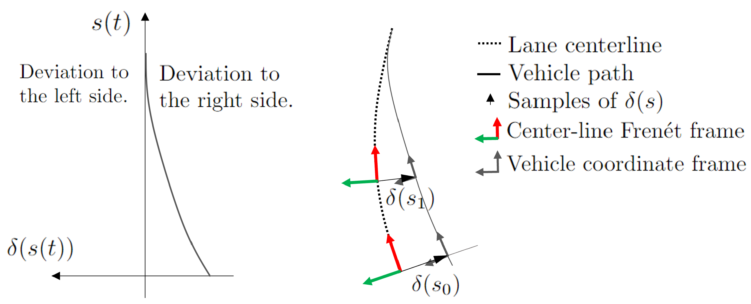
2.1. Lane Offset Modeling

The path, and hence the position of the vehicle in the lane, is often described by the position offset to the centerline of the lane (1).

$${\delta }^{\mathrm{Fr}}\left(t\right)\equiv \delta \left(t\right)$$

(1)

which is the lane offset value given in the Frenét-frame of the center line. An illustration is shown in Figure 1.

The lane offset is calculated by the driver model. This is a commonly followed approach by literature solutions [3,5,12], where the lane offset is only calculated in nominated node points. Then, a curve is fitted onto these points to formulate the locally planned path (2).

$$p^{\mathrm{path}}(t,x)=g({\left\{p_i^{\mathrm{np}}\left(t\right)\right\}}_{i=1}^n,\beta )$$

(2)

where $\beta$ are the curve parameters, $p_i^{\mathrm{np}}\left(t\right)={\left[\begin{array}{cc}{x}_i^{\mathrm{np}}\left(t\right)& y_i^{\mathrm{np}}\left(t\right)\end{array}\right]}^{\top }$ are the node point coordinates in the local planning frame, with $0<i\le n$ and n is the number of node points. If reference node points are measured on the centerline (e.g., by a video camera), then

$$p_i^{\mathrm{np}}\left(t\right)=p_i^{\mathrm{np},\mathrm{ref}}+\Delta p_i\left(t\right)$$

(3)

where

$$\Delta p_i\left(t\right)=\left[\begin{array}{c}-sin({\mathsf{\Theta }}_i^{\mathrm{np},\mathrm{ref}}\left(t\right)){\delta }_i\left(t\right)\\ cos({\mathsf{\Theta }}_i^{\mathrm{np},\mathrm{ref}}\left(t\right)){\delta }_i\left(t\right)\end{array}\right]$$

(4)

with

$$d_i^{\mathrm{np},\mathrm{ref}}\left(t\right)={\parallel {\{p_i^{\mathrm{np},\mathrm{ref}}\left(t\right)\}}_{i=1}^n\parallel }_2$$

(5)

where ${\mathsf{\Theta }}_i^{\mathrm{np},\mathrm{ref}}$ is the orientation of the lane at node point i, and $d_i^{\mathrm{np},\mathrm{ref}}\left(t\right)$ is the distance of node point i from the origin of the planning frame. Therefore, the path planning problem of (2) is translated to the lane offset estimation problem (6).

$${\delta }_i\left(t\right)=f_i(u\left(t\right),{\delta }_i\left(t\right)):{\mathbb{R}}^m\mapsto \mathbb{R}$$

(6)

where $u\left(t\right)$ is the input vector, m is the number of inputs, and

$$\delta \left(t\right)=\left[\begin{array}{cccc}{\delta }_1\left(t\right)& {\delta }_2\left(t\right)& \cdots & {\delta }_n\left(t\right)\end{array}\right]\in {\mathbb{R}}^n$$

(7)

There are different solutions in the literature to estimate the lane offset. A few approaches propose neural network structures [3,4,5]. However, the training of these models is long, and they cannot be used to directly define the reference driver groups. Instead, we chose the Extended Linear Driver Model (ELDM) structure [12]. This is a linear, static parametric model. This model calculates the lane offset in the node points at even time steps. Supposing we have samples of the inputs at even time steps $T_s$, the lane offset is also updated periodically. Equation (6) is rewritten to the discrete time domain at the $k^{\mathrm{th}}$ step:

$${\delta }_{i,k}={\widehat{f}}_i(u_k,u_{k-1}\cdots u_{k-n_u},{\delta }_{i,k-1},{\delta }_{i,k-2}\cdots {\delta }_{i,k-n_{\delta }})+e_{i,k}$$

(8)

where ${\delta }_{i,k}=\delta \left(k{T}_s\right)$ and $u_k=u\left(k{T}_s\right)$ the samples of the lane offset and the input vector, $e_{i,k}$ is the fit error and ${\widehat{f}}_i$ is the function approximate of $f_i\left(·\right)$, $n_u$ and $n_{\delta }$ are the time window sizes of the inputs and lane offset, respectively. The LDM model equation is given in (9).

$${\mathcal{M}}^{\mathrm{LDM}}:{\widehat{f}}_i={\delta }_{i,k}^{\mathrm{left}}+{\delta }_{i,k}^{\mathrm{right}}+{\delta }_0=u_{i,k}^{\mathrm{left}}{P}^{\mathrm{left}}+u_{i,k}^{\mathrm{right}}{P}^{\mathrm{right}}+{\delta }_0$$

(9)

The straight line distance is denoted by ${\delta }_0$. $n_u=1$, $n_{\delta }=0$, and $n=3$ according to [12]. Thus, $P^{\mathrm{left}},P^{\mathrm{right}}\in {\mathbb{R}}^{3\times 3}$. The node points are nominated at a constant distance from the origin of the planning frame [18]:

$$d^{\mathrm{np},\mathrm{ref}}\left(t\right)\equiv d^{\mathrm{np},\mathrm{ref}}=\left[\begin{array}{ccc}10.0& 39.0& 136.0\end{array}\right]m$$

(10)

The input of the model is three average curvature values between the origin of the planning frame and the first, second, and third node points. The values are distinguished between left and right curve situations, which are calculated based on the average preview curvature $\kappa \left(t\right)$:

$$\begin{array}{c}\hfill u_k^{\mathrm{left}}=\left\{\begin{array}{c}{\left[\begin{array}{ccc}{\kappa }_{\mathrm{o}1}& {\kappa }_{12}& {\kappa }_{23}\end{array}\right]}^{\top },\mathrm{if}{\displaystyle \frac{{\kappa }_{\mathrm{o}1}+{\kappa }_{12}+{\kappa }_{23}}{3}}>{\kappa }_{\min }\hfill \\ 0,\mathrm{otherwise}\hfill \end{array}\right.\\ \hfill u_k^{\mathrm{right}}=\left\{\begin{array}{c}{\left[\begin{array}{ccc}{\kappa }_{\mathrm{o}1}& {\kappa }_{12}& {\kappa }_{23}\end{array}\right]}^{\top },\mathrm{if}{\displaystyle \frac{{\kappa }_{\mathrm{o}1}+{\kappa }_{12}+{\kappa }_{23}}{3}}<-{\kappa }_{\min }\hfill \\ 0,\mathrm{otherwise}\hfill \end{array}\right.\end{array}$$

(11)

where ${\kappa }_{\min }$ is the minimum selected preview curvature. An example is shown in Figure 2 to illustrate the operation of the LDM. The vehicle is ahead of a left curve, positioned in the straight section leading up to the curve. In the preview distance, the curve is detected. The bottom plot shows the predicted curvature $\kappa \left(x\right)$ within this preview distance. The average road curvature values are calculated between the node points:

$$u_k={\left[\begin{array}{ccc}{\kappa }_{\mathrm{o}1,\mathrm{k}}\approxeq 0& {\kappa }_{12,\mathrm{k}}>0& {\kappa }_{23,\mathrm{k}}\gg 0\end{array}\right]}^{\top }$$

(12)

Let us consider the following settings for the model left curve parameters:

$$P^{\mathrm{left}}=\left[\begin{array}{ccc}1& -1& 0\\ 0& 1& -1\\ -1& 0& 1\end{array}\right]$$

(13)

and $P^{\mathrm{right}}={\left[\begin{array}{c}0\end{array}\right]}^{3\times 3}$ and ${\delta }_0=0$. By a simple calculation, we can see that using (13) in the scenario shown in Figure 2, the output offset vector is

$${\delta }_k={\left[\begin{array}{ccc}{\delta }_{1,k}<0& {\delta }_{2,k}\ll 0& {\delta }_{3,k}\gg 0\end{array}\right]}^{\top }$$

(14)

If a curve is fitted on these shifted node points, the red path from Figure 2 can be obtained. The idea is to fit the parameters to the measured data of human drivers.

2.2. Parameter Fitting

The LDM structure proposed in (9) is a linear model, whose parameters can be calculated by fitting the model to measured data. For this, the naturalistic driving of 30 drivers has been recorded [19]. This yields the following dataset, considering (11):

$$\begin{array}{c}\hfill {\mathcal{D}}^u={\{\{u_k^{\mathrm{left}},u_k^{\mathrm{right}}\}\}}_{k=1}^N{\mathcal{D}}^{\delta }={\left\{{\delta }_k\right\}}_{k=1}^N\end{array}$$

(15)

where N is the number of samples in the given measurement. When processing the data (15) the samples are ordered in matrix form (16).

$$D^u=\mathrm{col}\left({\mathcal{D}}^u\right)\in {\mathbb{R}}^{N\times 6}{D}^{\delta }=\mathrm{col}({\mathcal{D}}^{\delta })\in {\mathbb{R}}^{N\times 3}$$

(16)

Equation (9) can be rewritten in a compact form, using (16) and considering ${\delta }_0\equiv 0$ (i.e., the data is centralized):

$$D^{\delta }=\widehat{f}\left(u\right)+e=D^{u}P+e$$

(17)

where $P={\left[\begin{array}{cc}{P}^{\mathrm{left}}& P^{\mathrm{right}}\end{array}\right]}^{\top }\in {\mathbb{R}}^{6\times 3}$ is the model parameter matrix, and $e\in {\mathbb{R}}^{N\times 3}$ is the fit error. The model parameters can be calculated by minimizing a pre-selected objective function, considering $e_i=e[:,i]$, i.e., the $i^{\mathrm{th}}$ column of e:

$$\arg \min \left\{e_i^{\top }{e}_i\right|D^u,D_i^{\delta }\}=\arg \min \{V({\widehat{f}}_i,D^u,D_i^{\delta })\}$$

(18)

The objective function $V\left(·\right)$ is formulated in a way to minimize the least squares error between the function estimate and the training data:

$$V({\widehat{f}}_i,D^u,D_i^{\delta })={({\delta }_i-D^u{P}_i)}^{\top }({\delta }_i-D^u{P}_i)$$

(19)

where $P_i=P[:,i]$, i.e., the $i^{\mathrm{th}}$ column of the parameter matrix. Equation (19) can be solved in closed form to obtain the optimal value of $P_i$, using the pseudo inverse formulation of $D^u$:

$$P_i^{*}={\delta }_i{\left(D^u\right)}^{†}$$

(20)

From this, the optimal parameter matrix is formulated simply:

$$P^{*}=\left[\begin{array}{ccc}{P}_1^{*}& P_2^{*}& P_3^{*}\end{array}\right]$$

(21)

It can be shown that for all drivers, the parameter values reach their steady state well within the length of the data sequence. To prove that the regression is continuously executed on a gradually increasing subset of the data sequence (22).

$${\breve{P}}^{*}={\breve{\delta }}_i{({\breve{D}}^u)}^{†}$$

(22)

where ${\breve{\delta }}_i$ and ${\breve{D}}^u$ are the subsets of ${\delta }_i$ and $D^u$, in the $k^{\mathrm{th}}$ calculation cycle ${\breve{\delta }}_{i,k}={\delta }_i[1:k]$ and ${\breve{D}}_k^u=D^u[1:k,:]$. The convergence to steady state is calculated based on the error between the estimated parameters ${\breve{P}}^{*}$ and the reference parameters $P^{*}$. Then, the normalized RMS value of the estimation error is calculated (23).

$${\mathrm{NRMS}}_{{\breve{P}}^{*}}={\displaystyle \frac{\sqrt{{\parallel {\breve{P}}^{*}-P^{*}\parallel }_2}}{\max \left(P^{*}\right)-\min \left(P^{*}\right)}}$$

(23)

where ${\parallel {\breve{P}}^{*}-P^{*}\parallel }_2$ is the ${\ell }_2$ norm of the parameter estimation error.

2.3. Parameter Clustering

After the parameters of the model are calculated, they are used to cluster drivers into driver groups. Clustering is one of the most important techniques within the field of unsupervised learning and is used to group similar data points based on a distance metric. Three main types can be distinguished within clustering methods: hierarchical, center-based, and density-based clustering. In this paper, the center-based K-means clustering method is chosen [20], which is also used by many similar papers [13,14,15,21]. This method aims to choose a centroid for the parameters, which minimizes the criterion known as inertia. The K-means algorithm has one hyperparameter K, the number of clusters to be calculated. Choosing the right value of K is either heuristic (i.e., decision on cluster number as an empirical value), or optimizing an appropriately selected performance indicator. One of the most widely accepted indicators of the clustering performance is the silhouette coefficient [22]. The silhouette values for each sample in the dataset are calculated. The higher the average silhouette value for all elements, the better the clustering performance. The minimal requirement, which is often proposed by the literature, is to choose a value of K such that at least one element in each cluster would exceed the average silhouette value for all elements. Besides the hyperparameter K, the performance of the K-means algorithm is highly influenced by the choice of the distance calculation method. The distance of the elements in a multi-dimensional space is given by the norm of the error vector between the two elements. The most often used normalization methods are Euclidean (${\ell }_2$) norm and the Manhattan (${\ell }_1$) norm. As a result of clustering, each element of the input set is assigned to one specific cluster. In this application, the clustering equally means grouping the drivers who have a similar curve path selection policy. These drivers are then characterized by one behavior mode, which is given by the centroid of the cluster. Let us transform the parameter matrix P into a parameter vector:

$$p={\left[\begin{array}{ccc}P{[:,1]}^{\top }& P{[:,2]}^{\top }& P{[:,3]}^{\top }\end{array}\right]}^{\top }\in {\mathbb{R}}^{18}$$

(24)

It is noted that (24) is calculated for each driver individually, resulting in an individual parameter vector $p^{{\mathrm{dr}}_{\mathrm{j}}}$ for the $j^{\mathrm{th}}$ driver from the reference dataset. After clustering, there are K number of clusters. Let us denote the elements of cluster $c_{\gamma }$ by

$$c^{\gamma }=\left[\begin{array}{cccc}{p}^{{\mathrm{dr}}_1,\gamma }& p^{{\mathrm{dr}}_2,\gamma }& \cdots & p^{{\mathrm{dr}}_{\mathsf{\Gamma }},\gamma }\end{array}\right]$$

(25)

where $\mathsf{\Gamma }$ is the number of elements in $c^{\gamma }$. Then, this cluster, and as such this driver group, is characterized by the centroid parameter of the cluster $\gamma$, given in (26).

$$p^{\gamma }={\displaystyle \frac{1}{\mathsf{\Gamma }}}\sum _{j=1}^{\mathsf{\Gamma }}{p}^{{\mathrm{dr}}_j,\gamma }$$

(26)

Any driver given its parameter vector $p^{{\mathrm{dr}}_j}$ can be classified into clusters $c^{\gamma }$ by calculating the parameter error vector (27) to each centroid vector, and choosing the one it fits the most (28).

$$\Delta p^{{\mathrm{dr}}_j,\gamma }=p^{{\mathrm{dr}}_j}-p^{\gamma }$$

(27)

$${\widehat{c}}^{{\mathrm{dr}}_j}=\mathrm{loc}\left(\min \left({\parallel \Delta p^{{\mathrm{dr}}_j,\gamma }\parallel }_2\right)\right)$$

(28)

2.4. Online Parameter Identification

In order to use parameter calculation (20) all data points must be stored priorly. This hinders the algorithms from being used in embedded vehicle controllers, as the memory consumption is too high. Therefore, methods are sought to estimate the model parameter vector without the need to use too much memory. One of the most widely used parameter identification algorithms is the Kalman filter [16]. This filter was originally designed for linear systems, but has been extended to handle non-linear systems [23]. The modified structure is called the Extended Kalman Filter (EKF). Using EKF for parameter identification is a widely accepted technique. Papers propose to use the filter in the field of polymer technique [24], bioengineering [25], and radar technology [26]. Even though the model proposed in (17) is linear, the estimation of system parameters requires the augmentation of the model with the parameters as state variables, which hence becomes non-linear. The LDM model equations from (17) are rewritten in the form of (29).

$$\begin{array}{c}\hfill {\widehat{f}}_1:{\widehat{\delta }}_1=u_1^{\mathrm{left}}{\widehat{P}}_{11}+u_2^{\mathrm{left}}{\widehat{P}}_{21}+\cdots +u_3^{\mathrm{right}}{\widehat{P}}_{61}\\ \hfill {\widehat{f}}_2:{\widehat{\delta }}_2=u_1^{\mathrm{left}}{\widehat{P}}_{12}+u_2^{\mathrm{left}}{\widehat{P}}_{22}+\cdots +u_3^{\mathrm{right}}{\widehat{P}}_{62}\\ \hfill {\widehat{f}}_3:{\widehat{\delta }}_3=u_1^{\mathrm{left}}{\widehat{P}}_{13}+u_2^{\mathrm{left}}{\widehat{P}}_{23}+\cdots +u_3^{\mathrm{right}}{\widehat{P}}_{63}\end{array}$$

(29)

Based on the state Equation (29), the state vector is given by (30).

$$x={\left[\begin{array}{ccc}{\widehat{\delta }}_1& {\widehat{\delta }}_2& {\widehat{\delta }}_3\end{array}\right]}^{\top }$$

(30)

The augmentation means extending the state vector by adding the parameters as states. This way, the steady-state value of the parameters is observed via state estimation. As the model ${\mathcal{M}}^{\mathrm{LDM}}$ is considered to be linear and time invariant, the parameters are constant; therefore, the estimation of the steady state equally means the final parameter values. The augmented state equations $\widehat{f}(x,u)$ are given by (31).

$$\begin{array}{c}\hfill {\widehat{f}}_1:{\widehat{\delta }}_1=u_1^{\mathrm{left}}{\widehat{P}}_{11}+u_2^{\mathrm{left}}{\widehat{P}}_{21}+\cdots +u_3^{\mathrm{right}}{\widehat{P}}_{61}\\ \hfill {\widehat{f}}_2:{\widehat{\delta }}_2=u_1^{\mathrm{left}}{\widehat{P}}_{12}+u_2^{\mathrm{left}}{\widehat{P}}_{22}+\cdots +u_3^{\mathrm{right}}{\widehat{P}}_{62}\\ \hfill {\widehat{f}}_3:{\widehat{\delta }}_3=u_1^{\mathrm{left}}{\widehat{P}}_{13}+u_2^{\mathrm{left}}{\widehat{P}}_{23}+\cdots +u_3^{\mathrm{right}}{\widehat{P}}_{63}\\ \hfill {\widehat{f}}_4:{\widehat{P}}_{11}={\widehat{P}}_{11}\\ \hfill ⋮\\ \hfill {\widehat{f}}_{21}:{\widehat{P}}_{63}={\widehat{P}}_{63}\end{array}$$

(31)

Then, the augmented state vector is given by (32)

$$x^{\prime }={\left[\begin{array}{cccccccc}{\widehat{\delta }}_1& {\widehat{\delta }}_2& {\widehat{\delta }}_3& {\widehat{P}}_{11}& {\widehat{P}}_{12}& \cdots & & {\widehat{P}}_{63}\end{array}\right]}^{\top }\in {\mathbb{R}}^{21}$$

(32)

where $\widehat{P}$ qualifies as the estimated parameter vector. The augmented system is non-linear, as ${\widehat{f}}_1$ — ${\widehat{f}}_3$ contains the multiplication of state variables ${\widehat{P}}_{11}$ — ${\widehat{P}}_{61}$ and the input variables $u_1$ — $u_6$. Therefore, the usage of EKF is necessary, linearizing the system at cycle k around the augmented state $x_k^{\prime }$ and the input $u_k^{\mathrm{left}}$ and $u_k^{\mathrm{right}}$. The system and the input matrices are given by (33).

$$F_k={\left[\begin{array}{c}{\displaystyle \frac{\partial {\widehat{f}}_i}{\partial x_j^{\prime }}}\end{array}\right]}_{x_k^{\prime },u_k^{\mathrm{left}},u_k^{\mathrm{right}}}\in {\mathbb{R}}^{21\times 21}{G}_k={\left[\begin{array}{c}{\displaystyle \frac{\partial {\widehat{f}}_i}{\partial u_j}}\end{array}\right]}_{x_k^{\prime },u_k^{\mathrm{left}},u_k^{\mathrm{right}}}\in {\mathbb{R}}^{21\times 3}$$

(33)

The system output equations $\widehat{h}\left(x^{\prime }\right)$ are given by (34).

$$\begin{array}{c}\hfill {\widehat{h}}_1:{\widehat{\delta }}_1={\widehat{\delta }}_1\\ \hfill {\widehat{h}}_2:{\widehat{\delta }}_2={\widehat{\delta }}_2\\ \hfill {\widehat{h}}_3:{\widehat{\delta }}_3={\widehat{\delta }}_3\end{array}$$

(34)

The linearized system output matrix is given by (35).

$$H_k={\left[\begin{array}{c}{\displaystyle \frac{\partial {\widehat{h}}_i}{\partial x_j^{\prime }}}\end{array}\right]}_{x_k^{\prime },u_k^{\mathrm{left}},u_k^{\mathrm{right}}}\in {\mathbb{R}}^{3\times 21}$$

(35)

The EKF uses the linearized system to predict the expected value of the states and their covariance. The filtering steps are given in

Table 1. EKF Algorithm steps.

Step 0: Initialization

${\Sigma }_0$ and $x_0$

Step 1: Prediction (prior estimates)

$x_{k|k-1}=f(x_{k-1|k-1},u_k)$

${\Sigma }_{k|k-1}=F_k{\Sigma }_{k-1|k-1}{F}_k^T+Q$

Step 2: Kalman gain calculation

$K_k={\Sigma }_{k|k-1}{H}_k^T(H_k{\Sigma }_{k|k-1}{H}_k^T+R)$

Step 3: Correction (posterior estimates)

$x_{k|k}=x_{k|k-1}+K_k(z_k-h\left(x_{k|k}\right))$

${\Sigma }_{k|k}=(I-K_k{H}_k){\Sigma }_{k|k-1}$

, where $\Sigma$ is the state covariance matrix, $I\in {\mathbb{R}}^{21\times 21}$ is a unity matrix, z is the observed output vector. K is the Kalman gain. Q and R are the covariance matrix of the state model and the observation, respectively. It is noted that notation k is exchanged to $k|k$ and $k|k-1$. This is performed as the Kalman filter includes the calculation of the conditional probability of the state values; therefore, the previous estimates are considered to give the prior estimates in the prediction step, while the predicted estimates are used to calculate the correction, to give the posterior estimates. For simplification $x^{\prime }\equiv x$, $\widehat{f}\equiv f$ and $\widehat{h}\equiv h$.

The model and observation covariance matrices Q and R are to be tuned to yield the optimal estimation performance of the filter. The covariance matrices are simplified so that they would become diagonal, as given in (36).

$$Q=\left[\begin{array}{cc}{I}^{3\times 3}{\sigma }_y^2& O^{3\times 18}\\ O^{18\times 3}& I^{18\times 18}{\sigma }_p^2\end{array}\right]R=\left[\begin{array}{c}{I}^{3\times 3}{r}_y^2\end{array}\right]$$

(36)

In most applications, selecting the proper covariance values is critical. Often, covariance values are calculated to maximize the logarithmic likelihood of the predicted outputs, which is usually referred to as Maximum Likelihood Estimates (MLE).

$$\ell =\sum _{j=1}^k\log \left(p\left(x_j\right|x_1^{\prime },\cdots ,x_{j-1})\right)$$

(37)

The likelihood of state $x_k^{\prime }$ is calculated as the conditional probability on previous states, as given in (37), which can be formulated for Table 1 filter equations, as given in (38).

$$\ell ={\ell }_0+\sum _{j=1}^k\log \left(\right|{\Sigma }_y\left|\right)+y_{er{r}_j}{\Sigma }_y^{-1}{y}_{er{r}_j}$$

(38)

with ${\Sigma }_y=H{\Sigma }_{k|k-1}{H}^{\top }+R$ and $y_{er{r}_k}=z_k-h\left(x_{k|k}\right)$. ${\ell }_0$ is the initial likelihood estimate. The optimization problem of the covariance ${\sigma }_y$, ${\sigma }_p$ and $r_y$ is formulated in (39). Optimization is performed using the fmincon() function of MATLAB 2024b.

$$\begin{array}{cccc}\hfill {\displaystyle \underset{{\sigma }_y,{\sigma }_p,r_y}{min}}& \multicolumn{3}{c}{-\ell ({\sigma }_y,{\sigma }_p,r_y)}\\ \hfill \mathrm{s}.\mathrm{t}.& \hfill {\sigma }_y,{\sigma }_p,r_y\ge 0\end{array}$$

(39)

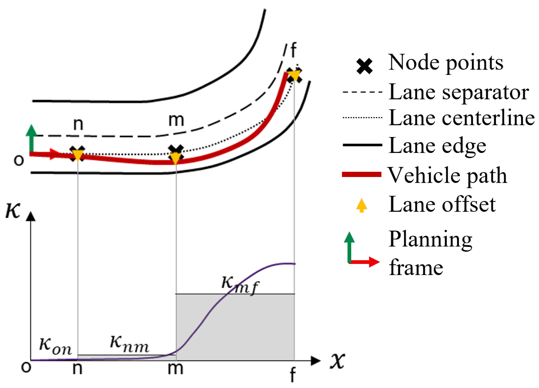
2.5. Path Planning

Once the LDM parameters are calculated (let it be individual or cluster centroid parameters), the lane offset vector (17) and the node point positions are calculated (3). A curve is fitted on the node points to yield the locally planned path (2). Some of the path planning papers use clothoid curves [27,28], splines [29,30,31] or polynomials [32,33,34]. Polynomials are simple but robust solution in terms of curve fitting. To illustrate the results of the driver model, a 3rd-order polynomial is fitted onto the node points. The polynomial path equation in the local planning coordinate frame $x-y$ is given in (40).

$$y_{path}\left(x\right)=a_0+a_{1}x+a_2{x}^2+a_3{x}^3$$

(40)

The polynomial coefficients $a_i$ are calculated using the MATLAB function polyfit.

3. Results

3.1. Dataset

In our study, the Human-like Behavior for Automated Driving (HLB4AV) dataset is used [19]. This dataset contains the driving data of 30 drivers, each driver driving the same test route, a rural road segment with a length of approximately 40 km. There are no urban sections nor highway sections in this database. The route is a two-lane road without a physical separation between them. The dataset contains the vehicle kinematic data (e.g., velocity, acceleration, and yaw rate), high precision GNSS data, lane information, i.e., the position of the lane edges, their relative orientation to the vehicle, and the curvature at the vehicle position. This dataset was specifically recorded for lane driving analysis, with various different drivers. 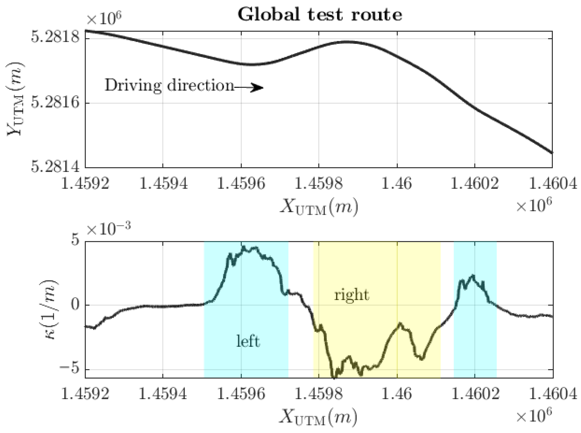In contrast to similar datasets, such as the Automated Vehicle Technologies (AVT) dataset [35] or the Strategic Highway Research Program (SHRP2) database [36], HLB4AV is available publicly. There are other public driving datasets, however these mostly contain accident data [37,38], or other very specific use case data [39]. Therefore, we use HLB4AV to fit the models and to generate the driver clustering results.

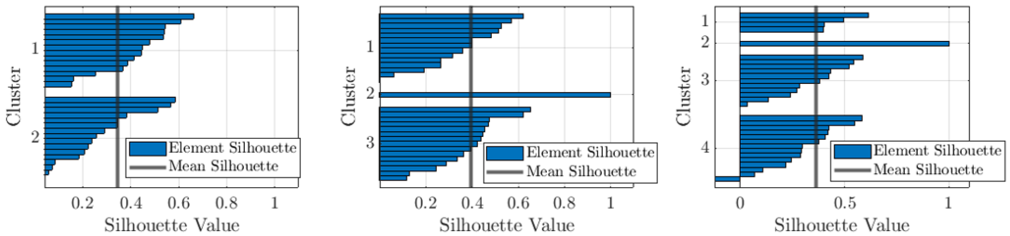
3.2. Driver Clustering

Data of the Human-like Behavior for Automated Vehicles (HLB4AV) dataset is used [19]. This dataset contains the naturalistic driving data of 30 drivers. The participants drove approximately 40 km on a rural road, with two lanes, without physical separation between the lanes. The driving does not contain urban or highway scenarios. The parameters of LDM were calculated by applying (20) on the drivers’ data, individually. Euclidean distance metric (${\mathit{\ell }}_2$) is chosen, as no significant differences have been observed when using other metrics. The number of clusters K is chosen by testing different values and comparing the silhouette values of the clusters. The values $K=\{2,3,4\}$ have been tested. The results are shown in Figure 3. In the case of $K=2$ there are multiple elements in both clusters that are well above the mean silhouette values. In cluster 2, there are a few elements with low silhouette values, though. In the case of $K=3$ there are no elements with negative silhouette values, the lowest is around $s=0.08$ in cluster 1 and $s=0.1$ in cluster 3. In cluster 2, there is only one element, which can be treated as an outlier. For $K=4$, cluster 2 is an outlier, while cluster 4 contains elements with very low silhouette values.

Based on the tests, $K=3$ clusters are chosen, which complies with similar papers [13,15,40], with a note that cluster 2 may be a group of outliers—the number of elements in this group is very low. The cluster centroids for clusters 1 and 3 are calculated based on (26), and are given in (41).

$$\begin{array}{c}\hfill P^1=\left[\begin{array}{cccccc}-0.10& 0.18& -0.05& -0.06& 0.28& -0.06\\ -0.52& 0.47& -0.06& -0.53& 0.57& -0.05\\ 0.12& -0.13& 0.03& 0.48& -0.43& 0.13\end{array}\right]\\ \hfill P^3=\left[\begin{array}{cccccc}0.44& -0.10& -0.04& 0.39& 0.04& -0.06\\ -0.06& 0.27& -0.05& -0.32& 0.53& -0.06\\ 0.11& -0.07& 0.09& 0.46& -0.44& 0.18\end{array}\right]\end{array}$$

(41)

The cluster parameters are used to plan the local path, as introduced in Section 2.5. The vehicle movement is simulated to be ideal (tracking error is zero), and the global path of the vehicle is analyzed. Simulations are run in MATLAB. The reference route is shown in Figure 4. First, there is a straight section, after which an S-curve (first left, then right) part follows. Then, there are a small right and left curves, which are followed again by a straight section. This path is taken from a real measurement; the vehicle speed is set based on the original measured speed. After the simulation, the planned offset to the lane is calculated. The results are shown in Figure 1.

The resulting clusters are groups of drivers, presumably with similar behavior in their curve path selection. However, we want to also formulate features of each group that define not only numerical similarity between the drivers but also similarity in their behavior of driving. Figure 5 shows the offset-time plot. Cluster 2 contains the data of driver 2 only and produces an outlying behavior. Cluster 3 drivers cut the curve significantly, symmetrically in left and right curves (the peak of the lane offset is similar). In general, these drivers drive closer to the opposite lane. Cluster 1 drivers have much lower curve cut, especially in the left curve. Drivers are slightly different in terms of the curve entry behavior; however, the difference is not significant. In the case of both cluster 1 and 3, there is a small negative offset before the left curve, which means the vehicle is on the outer side of the lane before turning in and cutting the curve.

Based on the observations, we propose features of each cluster, and based on the features, driving styles are defined. The results are shown in

Table 2. Driving cluster features and driving styles associated with them.

Feature	Cluster 1	Cluster 3
Curve cutting extent—left curve	low	high
Curve cutting extent—right curve	moderate	high
Curve entry outer driving	moderate	moderate
Driving style	cautious	dynamic

. There are two styles that are named empirically: dynamic (cluster 1) and cautious (cluster 2) drivers.

One more analysis is conducted by considering the cautious and dynamic groups. The kinematic primitives (e.g., mean velocity, maximum longitudinal and lateral acceleration) are compared. Such quantities are also proposed by the literature [14,15,40]. The results are given in

Table 3. Comparison of the clusters based on primitive kinematic features of the cluster elements. Bold quantities highlight that cluster 3 has a more dynamic behavior from kinematic point of view.

	${\overline{\mathit{v}}}_{\mathit{x}}$	$\mathbf{max}\left({\mathit{v}}_{\mathit{x}}\right)$	$\mathbf{min}\left({\mathit{a}}_{\mathit{x}}\right)$	$\mathbf{max}\left({\mathit{a}}_{\mathit{x}}\right)$	$\overline{|{\mathit{a}}_{\mathit{x}}|}$	$\overline{|{\mathit{a}}_{\mathit{y}}|}$
Cluster 1 (cautious)	23.62	30.35	−4.09	3.29	0.29	0.32
Cluster 3 (dynamic)	23.50	33.06	−6.28	5.92	0.75	0.35

. Considering the average speed and the average lateral acceleration, no significant change can be observed between the clusters. It is noted that the speed is also influenced by the traffic, which may be significantly different between the test drives. On the other hand, the maximum velocity, the highest deceleration and acceleration, as well as the average longitudinal absolute acceleration, are significantly different from each other. That means, the dynamic drivers are also more dynamic considering the general vehicle kinematics, further proving that the aforementioned clustering can indeed separate different driving styles. From practical utilization perspectives, the dynamic driving group must be analyzed to ensure that, in the event of reproducing this behavior, the system would not lead to unsafe scenarios. The standard lane width on the test route was $3.8$ m, while the vehicle width is approximately $1.8$ m. Then, the maximum lane offset of approximately ±1 m of the dynamic group would mean that the edge of the vehicle exactly touches the edge of the lane. This is an acceptable behavior if there are no obstacles (e.g., oncoming traffic) in the other lane. Also, from the viewpoint of the dynamic driver, the behavior is understandable: he wants to use the entire space available. From the ADAS point of view, such a lane offset is usually not acceptable. There are two ways of tackling this: first, a limitation can be applied to the calculated lane offset, which can ensure that the ego vehicle would not get too close to other objects. Secondly, for up to SAE level 2 systems [41], the lane following function works in cooperation with the driver; therefore, a higher lane offset threshold can be defined in curve cutting scenarios, before the system starts to steer against the driver.

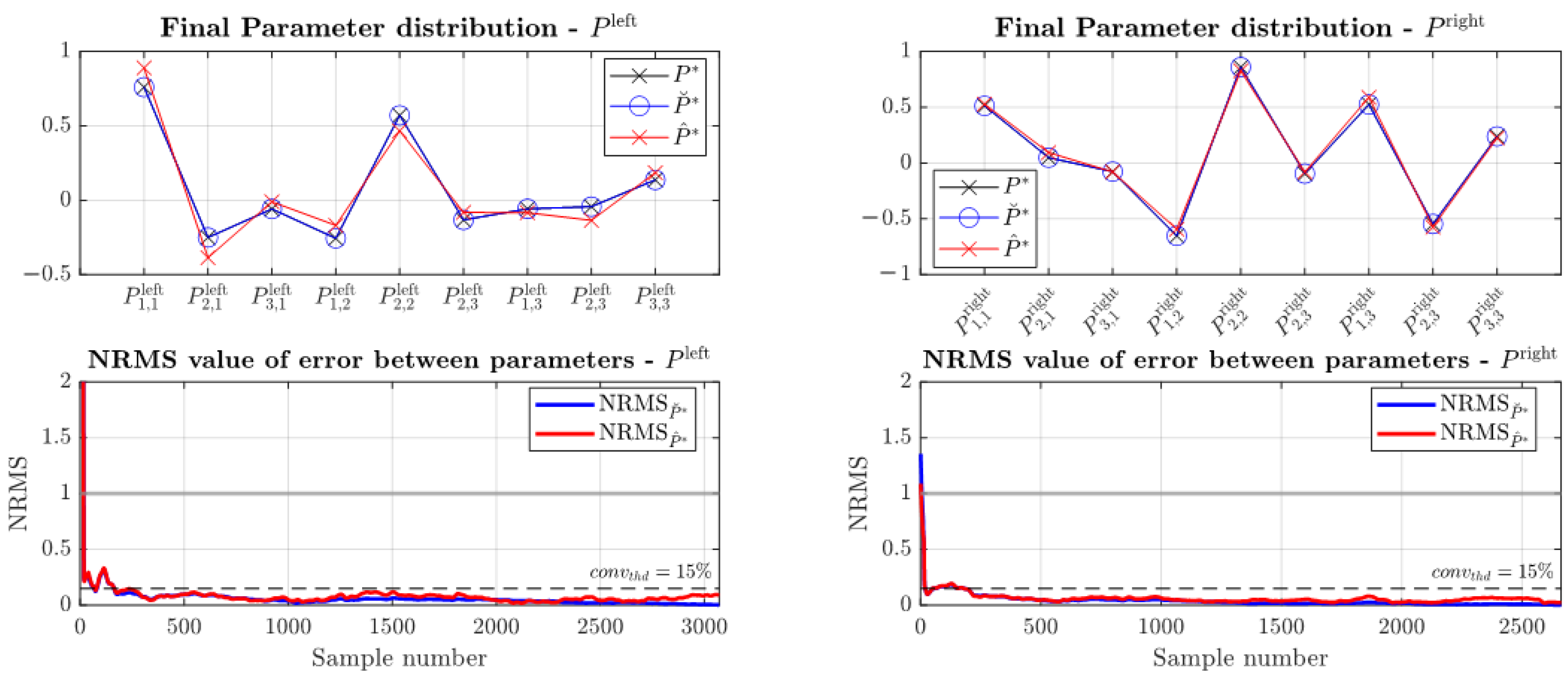
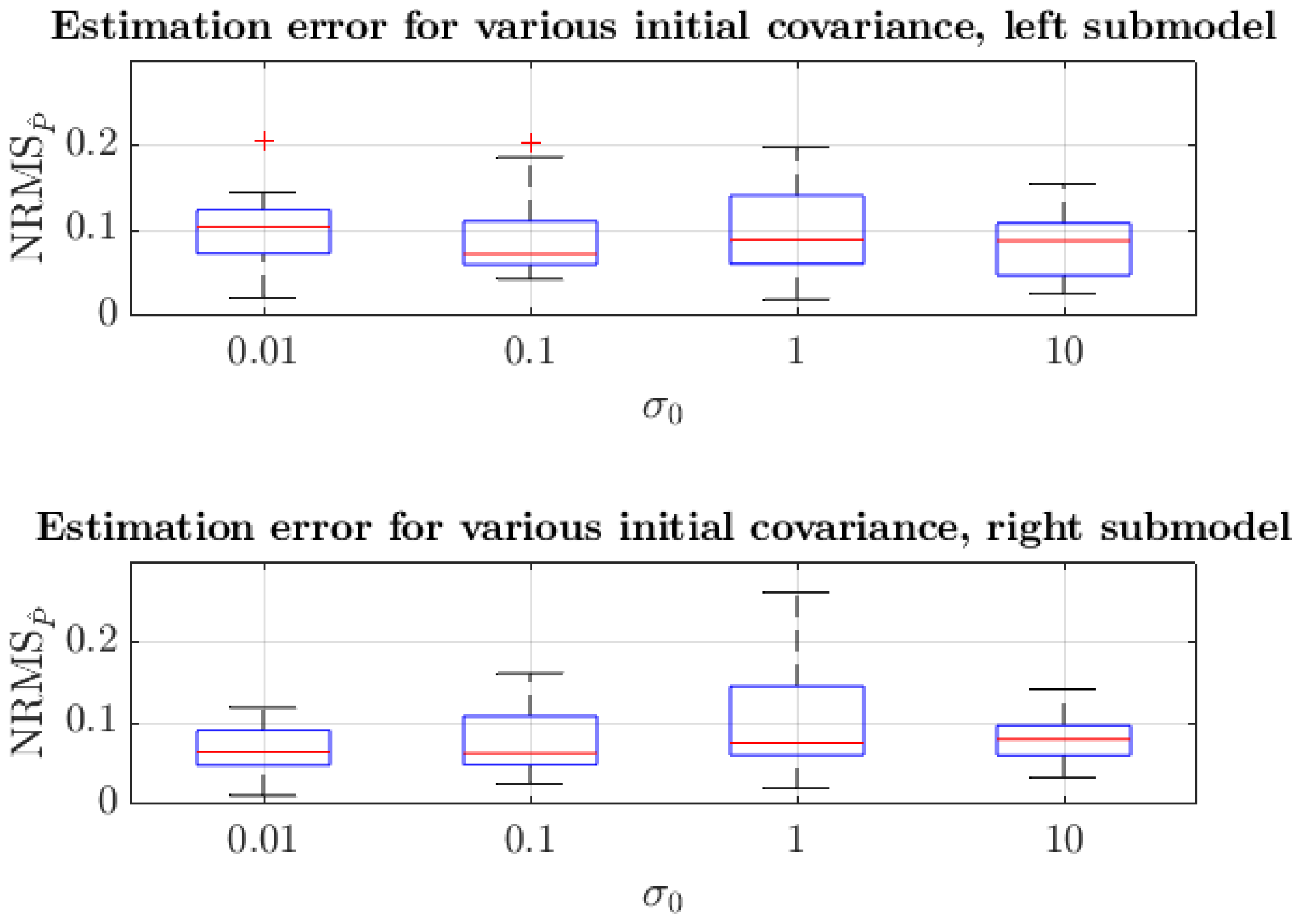
3.3. Online Parameter Learning

In the previous section, a dynamic and a cautious driving style group were defined. The reference parameter vectors are given in (26). In this section, we implement the EKF algorithm introduced in Section 2.4. To illustrate the algorithm’s accuracy, a test is executed. For this test, the data of driver no. 1 is taken from the reference dataset [19]. The parameters $P^{\mathrm{left}}$ and $P^{\mathrm{right}}$ are identified by the EKF algorithm. The initial guess of the outputs (i.e., the lane offset values) is taken from the first sample of the measurement, whereas the initial parameter values are assumed to be zero. The initial covariance matrix is given in (42).

$${\Sigma }_0=I^{21\times 21}{\sigma }_0^2$$

(42)

where ${\sigma }_0$ is the initial covariance value for all states, and ${\sigma }_0=0.1$ is chosen. The results of the test are shown in Figure 6. In the upper plots, the final estimate of the parameter vectors is visualized. Besides the estimator results ${\widehat{P}}^{*}$, the reference parameters $P^{*}$ calculated by (20) and the moving parameters ${\breve{P}}^{*}$ given in (22) are plotted. In the bottom plot, the NRMS values (23) of the parameter estimation error and the moving parameter error to the reference parameters are plotted. To help visualize $\mathrm{NRMS}=1$, a reference line is added to this plot. The results show that the EKF algorithm reaches convergence fast, together with the moving parameters. EKF algorithm estimates the parameter values with a small terminal error. Interestingly, the estimation error does not reach its minimum value at the very end of the simulation. The reason is that even the reference parameters change during driving as the behavior of the driver is not constant, either. The EKF can slowly react to these changes, but that causes a continuous rise and fall in the estimation error. In general, it is observed that the EKF can predict the parameter values accurately, giving a good basis for executing the classification based on the estimated parameters.

Further runs with different initial covariance values ${\sigma }_0$ have been conducted to prove the robustness of the algorithm. The results are shown in Figure 7. Selecting various initial covariances in the range of 0.01 and 10, the estimation error does not change significantly. This proves that the proposed EKF algorithm is robust against this parameter and may be applicable for real-time parameter learning.

3.4. Driver Classification

In Section 3.2, the drivers were clustered, and the centroid parameters of the clusters were calculated. In Section 3.3, it is shown that EKF has high estimation accuracy in terms of LDM parameters. The evaluation has been conducted based on the NRMS value of the estimation error. However, it is not trivial what impact an NRMS error of, e.g., 5% has on the classification output. In this section, the parameters estimated by EKF are used to classify the drivers into the clusters. The classification is performed based on the distance of the estimated parameter ${\widehat{P}}^{*}$ to cluster centroids given in (27) and (28). The same classification approach is applied using the reference parameters $P^{*}$. The classification results of the estimated and the reference parameters are compared. This way, the accuracy of EKF can be judged from an application point of view. The results are shown in

Table 4. Classification results of all drivers into driving style groups. Match means that classification based on the estimated parameters resulted in the same driving group as classification based on the reference parameters.

	Classification Results
Driver group match	27
Driver group mismatch	3

. The classification based on the estimated parameters succeeds in the case of 27 driver out of the 30 total drivers; hence, the accuracy is $90\%$. This may be improved by better estimation of the parameters or selecting a different classification approach.

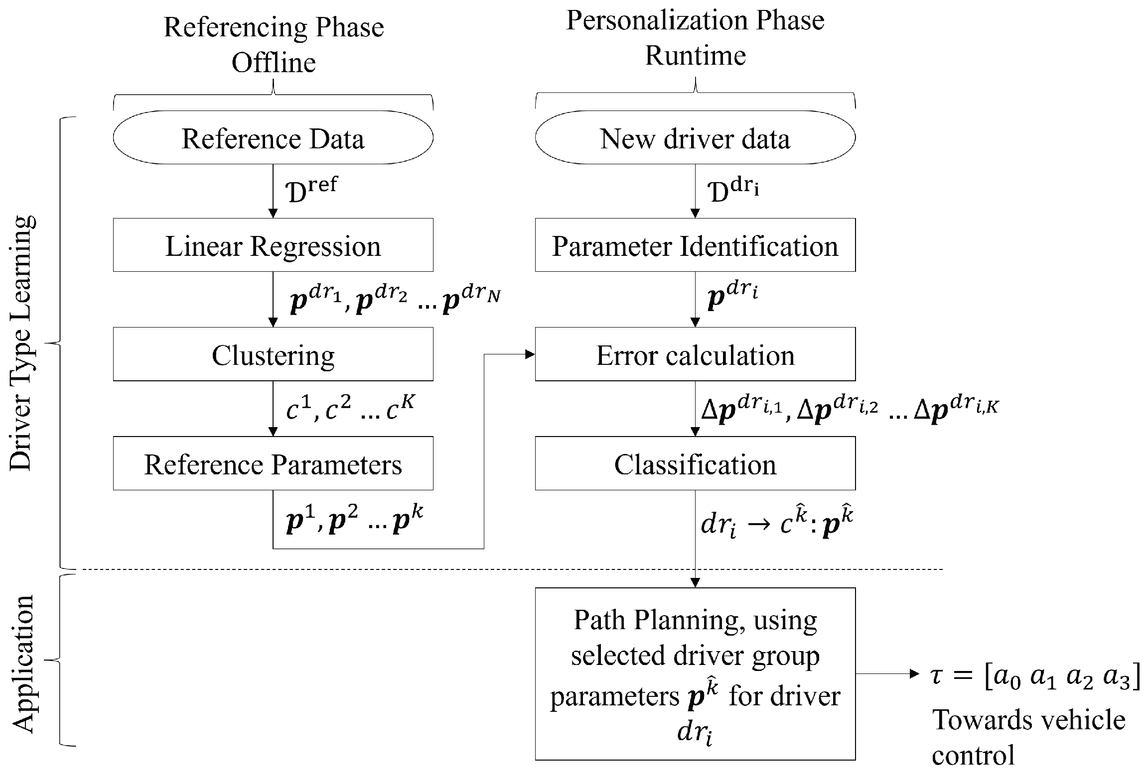
3.5. Proposed Workflow

In the previous sections, a proof of the personalization concept of lane centering systems has been introduced. Architecture-wise, a two-step approach is proposed:

1

Data of reference drivers ${\mathcal{D}}^{\mathrm{ref}}$ is collected, the LDM parameters of these drivers are calculated offline, using (20) to form the driver clusters $c=\left[\begin{array}{cccc}{c}_1& c_2& \cdots & c_K\end{array}\right]$. This is called the referencing phase.

2

Then, new test drivers, who are not part of the reference group, are measured, and their parameter vector is calculated online using the EKF algorithm given in Section 2.4. Using the identified parameter vector, the new driver is classified into one of the driving clusters (27) and (28). This is called the personalization phase.

This two-step approach is illustrated in Figure 8. In general, the proposed workflow can cover multiple curve driving styles, out of which in this study we identified two: dynamic and cautious. With the simple solution of EKF and the classification based on the parameter vector error to the cluster centroid parameters, implementation is possible even in environments with low available memory.

4. Conclusions

In this paper, we have collected existing solutions in the field of driver modeling, clustering and parameter identification to formulate a solution that can be used to make lane centering systems more human like. The following conclusions are drawn:

• Linear Driver Model (LDM), a simple, static, parametric model can be used to efficiently characterize drivers by their curve path preferences. The model parameters can be fitted on measured data and can be used to cluster drivers into a dynamic and a cautious driving style group.
• The curve driving groups identified by the LDM parameters are also separated by vehicle kinematics, therefore they are indeed dynamic and cautious drivers, not only from curve driving perspective but from motion perspective, too.
• Extended Kalman Filter can be used to learn the LDM parameters in an environment where memory consumption shall be low (e.g., in an embedded environment). With this, the real-time application of the proposed driver classification workflow is possible.

Our results prove that using simple solutions, personalization of lane centering systems is possible.

However, there are certain limitations of the work. The results were generated using a sample dataset of 30 drivers. Even though such an amount of data can be used to prove that the concept is right, further analysis could also show the robustness and applicability of the method better. Also, the planned path can be different from the actual path of the vehicle, if there is a real tracking control in the loop. The effect of both components must be studied together to show that the proposed method can be applied in a real automated driving chain. This is going to be in the focus of our next research step.

References

- Bongiorno, N.; Pellegrino, O.; Stuiver, A.; de Waard, D. Cumulative lateral position: A new measure for driver performance in curves. Traffic Saf. Res. 2022, 4, 20–34. [Google Scholar] [CrossRef]
- Qi, H.; Hu, X. Behavioral investigation of stochastic lateral wandering patterns in mixed traffic flow. Transp. Res. Part C 2023, 4, 104310. [Google Scholar] [CrossRef]
- Aoxue, L.; Haobin, J.; Li, Z.; Zhou, J.; Zhou, X. Human-Like Trajectory Planning on Curved Road: Learning From Human Drivers. IEEE Trans. Intell. Transp. Syst. 2020, 21, 3388–3397. [Google Scholar]
- Li, A.; Jiang, H.; Zhou, J.; Zhou, X. Learning Human-Like Trajectory Planning on Urban Two-Lane Curved Roads From Experienced Drivers. IEEE Access 2016, 4, 65828–65838. [Google Scholar] [CrossRef]
- Zhao, J.; Song, D.; Zhu, B.; Sun, Z.; Han, J.; Sun, Y. A Human-Like Trajectory Planning Method on a Curve Based on the Driver Preview Mechanism. IEEE Trans. Intell. Transp. Syst. 2023, 24, 11682–11698. [Google Scholar] [CrossRef]
- Chen, S.; Cheng, K.; Yang, J.; Zang, X.; Luo, Q.; Li, J. Driving Behavior Risk Measurement and Cluster Analysis Driven by Vehicle Trajectory Data. Appl. Sci. 2023, 13, 5675. [Google Scholar] [CrossRef]
- Conlter, R.C. Implementation of the Pure Pursuit Path Tracking Algorithm; Defense Technical Information Center: Fort Belvoir, VA, USA, 1992. [Google Scholar]
- McAdam, C.C. An Optimal Preview Control for Linear Systems. J. Dyn. Syst. Meas. Control. 1980, 102, 188–190. Available online: https://hdl.handle.net/2027.42/65011 (accessed on 5 May 2025). [CrossRef]
- Jiang, H.; Tian, H.; Hua, Y. Model predictive driver model considering the steering characteristics of the skilled drivers. Adv. Mech. Eng. 2019, 11, 1687814019829337. [Google Scholar] [CrossRef]
- Ungoren, A.Y.; Peng, H. An adaptive lateral preview driver model. Veh. Syst. Dyn. 2005, 43, 245–259. [Google Scholar] [CrossRef]
- Hess, R.; Modjtahedzadeh, A. A control theoretic model of driver steering behavior. IEEE Control. Syst. Mag. 1990, 10, 3–8. [Google Scholar] [CrossRef]
- Igneczi, G.; Horvath, E.; Toth, R.; Nyilas, K. Curve Trajectory Model for Human Preferred Path Planning of Automated Vehicles. Automot. Innov. 2023, 1, 50–60. [Google Scholar] [CrossRef]
- de Zepeda, M.V.N.; Meng, F.; Su, J.; Zeng, X.J.; Wang, Q. Dynamic clustering analysis for driving styles identification. Eng. Appl. Artif. Intell. 2021, 97, 104096–104105. [Google Scholar] [CrossRef]
- Lina, X.; Zejun, K. Driving Style Recognition Model Based on NEV High-Frequency Big Data and Joint Distribution Feature Parameters. World Electr. Veh. J. 2021, 12, 142. [Google Scholar] [CrossRef]
- Chu, D.; Deng, Z.; He, Y.; Wu, C.; Sun, C.; Lu, Z. Curve speed model for driver assistance based on driving style classification. IET Intell. Transp. Syst. 2017, 11, 501–510. [Google Scholar] [CrossRef]
- Kalman, R.E. A New Approach to Linear Filtering and Prediction Problems. Trans. ASME—J. Basic Eng. 1960, 82, 35–45. [Google Scholar] [CrossRef]
- Zhao, Y.; Chevrel, P.; Claveau, F.; Mars, F. Continuous Identification of Driver Model Parameters via the Unscented Kalman Filter. IFAC-Pap. Online 2019, 52, 126–133. [Google Scholar] [CrossRef]
- Igneczi, G.F.; Horvath, E. Node Point Optimization for Local Trajectory Planners based on Human Preferences. In Proceedings of the IEEE 21st World Symposium on Applied Machine Intelligence and Informatics, Herl’any, Slovakia, 19–21 January 2023; pp. 1–6. [Google Scholar]
- Gergo, I.; Erno, H. Human-Like Behaviour for Automated Vehicles (HLB4AV) Naturalistic Driving Dataset. In Proceedings of the 2024 IEEE 22nd Jubilee International Symposium on Intelligent Systems and Informatics (SISY), Pula, Croatia, 19–21 September 2024. [Google Scholar]
- Hartigan, J.A. Clustering Algorithms, 99th ed.; John Wiley & Sons, Inc.: New York, NY, USA, 1975. [Google Scholar]
- Cristian-David, R.L.; Carlos-Andres, G.M.; Carlos-Anibal, C.V. Classification of Driver Behavior in Horizontal Curves of Two-Lane Rural Roads. Rev. Fac. Ing. 2021, 30. [Google Scholar] [CrossRef]
- Kaufman, L.; Rousseeuw, P. Finding Groups in Data: An Introduction To Cluster Analysis; John Wiley & Sons: Hoboken, NJ, USA, 1990. [Google Scholar] [CrossRef]
- Li, X.; Lei, A.; Zhu, L.; Ban, M. Improving Kalman filter for cyber physical systems subject to replay attacks: An attack-detection-based compensation strategy. Appl. Math. Comput. 2023, 466, 128444. [Google Scholar] [CrossRef]
- Semino, D.; Moretta, M.; Scali, C. Parameter estimation in Extended Kalman Filters for quality control in polymerization reactors. Comput. Chem. Eng. 1996, 20, 913–918. [Google Scholar] [CrossRef]
- Sun, X.; Jin, L.; Xiong, M. Extended Kalman Filter for Estimation of Parameters in Nonlinear State-Space Models of Biochemical Networks. PLoS ONE 2023, 3, e3758. [Google Scholar] [CrossRef]
- Na, W.; Yoo, C. Real-Time Parameter Estimation of a Dual-Pol Radar Rain Rate Estimator Using the Extended Kalman Filter. Remote Sens. 2021, 13, 2365. [Google Scholar] [CrossRef]
- Gackstatter, C.; Heinemann, P.; Thomas, S.; Klinker, G. Stable Road Lane Model Based on Clothoids. In Advanced Microsystems for Automotive Applications 2010: Smart Systems for Green Cars and Safe Mobility; Springer: Berlin/Heidelberg, Germany, 2010; pp. 133–143. [Google Scholar] [CrossRef]
- Fatemi, M.; Hammarstrand, L.; Svensson, L.; García-Fernández, Á.F. Road geometry estimation using a precise clothoid road model and observations of moving vehicles. In Proceedings of the 17th International IEEE Conference on Intelligent Transportation Systems (ITSC), Qingdao, China, 8–11 October 2014; pp. 238–244. [Google Scholar] [CrossRef]
- Götte, C.; Keller, M.; Nattermann, T.; Haß, C.; Glander, K.H.; Bertram, T. Spline-Based Motion Planning for Automated Driving. IFAC-Pap. Online 2017, 50, 9114–9119. [Google Scholar] [CrossRef]
- Xu, W.; Wang, Q.; Dolan, J.M. Autonomous Vehicle Motion Planning via Recurrent Spline Optimization. In Proceedings of the 2021 IEEE International Conference on Robotics and Automation (ICRA), Xi’an, China, 30 May–5 June 2021; pp. 7730–7736. [Google Scholar] [CrossRef]
- Wang, Y.; Shen, D.; Teoh, K. Lane detection using spline model. Pattern Recognit. Lett. 2000, 21, 677–689. [Google Scholar] [CrossRef]
- Moritz, W.; Julius, Z.; Sören, K.; Sebastian, T. Optimal Trajectory Generation for Dynamic Street Scenarios in a Frenét Frame. In Proceedings of the IEEE International Conference on Robotics and Automation, Anchorage, AK, USA, 3–7 May 2010; pp. 987–993. [Google Scholar]
- Papadimitriou, I.; Tomizuka, M. Fast lane changing computations using polynomials. In Proceedings of the 2003 American Control Conference, Denver, CO, USA, 4–6 June 2003; Volume 1, pp. 48–53. [Google Scholar] [CrossRef]
- Nelson, W. Continuous-Curvature Paths for Autonomous Vehicles; AT&T Bell Laboratories: Murray Hill, NJ, USA, 1984. [Google Scholar] [CrossRef]
- Advanced Vehicle Tecnhologies Consortium. Advanced Vehicle Technology Consortium Dataset. 2024. Available online: https://avt.mit.edu/ (accessed on 15 April 2024).
- Strategic Highway Research Program by Virginia Tech Transportation Institute. The SHRP 2 Naturalistic Driving Study. 2012. Available online: https://insight.shrp2nds.us/ (accessed on 15 April 2024).
- Administration, Federal Motor Carrier Safety Data Repository of Naturalistic Driving and Other Dataset. 2023. Available online: https://fmcsadatarepository.vtti.vt.edu/ (accessed on 15 April 2024).
- Alam, M.R.; Batabyal, D.; Yang, K.; Brijs, T.; Antoniou, C. Application of naturalistic driving data: A systematic review and bibliometric analysis. Accid. Anal. Prev. 2023, 190, 107155. [Google Scholar] [CrossRef]
- Zheng, Y.; Shyrokau, B.; Keviczky, T. Reconstructed Roundabout Driving Dataset. 2021. Available online: https://dx.doi.org/10.21227/7t54-mt12 (accessed on 9 June 2025).
- Aydin, M.M. A new evaluation method to quantify drivers’ lane keeping behaviors on urban roads. Transp. Lett. 2020, 12, 738–749. [Google Scholar] [CrossRef]
- Society of Automobile Engineers International. Taxonomy and Definitions for Terms Related to Driving Automation Systems for On-Road Motor Vehicles J3016_202104; SAE Mobilus: Amsterdam, The Netherlands, 2021. [Google Scholar]