Abstract
Accurate wellbore trajectory prediction is of great significance for enhancing the efficiency and safety of directional drilling in coal mines. However, traditional mechanical analysis methods have high computational complexity, and the existing data-driven models cannot fully integrate non-sequential features such as stratum lithology. To solve these problems, this study proposes a parallel input gated recurrent unit (Pi-GRU) model based on the TensorFlow framework. The GRU network captures the temporal dependencies of sequence data (such as dip angle and azimuth angle), while the BP neural network extracts deep correlations from non-sequence features (such as stratum lithology), thereby achieving multi-source data fusion modeling. Orthogonal experimental design was adopted to optimize the model hyperparameters, and the ablation experiment confirmed the necessity of the parallel architecture. The experimental results obtained based on the data of a certain coal mine in Shanxi Province show that the mean square errors (MSE) of the azimuth and dip angle angles of the Pi-GRU model are 0.06° and 0.01°, respectively. Compared with the emerging CNN-BiLSTM model, they are reduced by 66.67% and 76.92%, respectively. To evaluate the generalization performance of the model, we conducted cross-scenario validation on the dataset of the Dehong Coal Mine. The results showed that even under unknown geological conditions, the Pi-GRU model could still maintain high-precision predictions. The Pi-GRU model not only outperforms existing methods in terms of prediction accuracy, with an inference delay of only 0.21 milliseconds, but also requires much less computing power for training and inference than the maximum computing power of the Jetson TX2 hardware. This proves that the model has good practicability and deployability in the engineering field. It provides a new idea for real-time wellbore trajectory correction in intelligent drilling systems and shows strong application potential in engineering applications.
1. Introduction
The precise control and accurate prediction of borehole trajectories are critical determinants in directional drilling operations, directly impacting drilling quality, optimizing operational efficiency, reducing costs, and ensuring safety in near-horizontal drilling scenarios. However, regardless of whether wired or electromagnetic wireless measurement-while-drilling (MWD) systems are employed, the sensors are invariably positioned behind screw drill tools. Moreover, owing to the use of magnetic sensors, a nonmagnetic drill collar (≥3 m in length) must be installed between the sensors and screw drill tools to eliminate magnetic interference from the drilling assembly. Consequently, the measurement point remains positioned more than 6 m behind the drill bit [1], creating a substantial blind zone when measuring borehole parameters. The screw motor adjusts the direction of the drill bit through the orientation of its front-end bent sub, with the bottom-hole assembly (BHA) configuration illustrated in Figure 1.
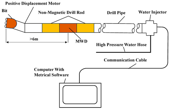
Figure 1.
Screw motor drilling tool assembly.
The traditional methods for predicting wellbore trajectories can be classified into two main categories: mechanical analysis methods and data-driven methods.
The existing mechanical analysis methods fall under three main types. (1) Mechanical interaction-based models, such as those proposed by Fischer et al. [2], integrate BHA stress distributions [3], deformation characteristics, and bit-rock interaction mechanisms to account for multifactor coupling effects. (2) Build-rate analysis methods, including the three-point geometry method [4], balanced curvature method [5], and limit curvature method [6], predict dip angle changes by calculating the build-up rate. (3) MWD-derived approaches [7], which utilize real-time trajectory parameters derived from MWD systems to forecast subsequent survey points, are typically implemented through techniques such as the average minimum curvature method [8] and radius of curvature method [9].
In addition to the challenges brought by complex geological conditions and real-time trajectory control, dynamic loads on the drill string (such as torsional vibration, axial impact, and lateral impact) also significantly affect drilling efficiency, tool life, and wellbore stability [10]. To mitigate these impacts, researchers have proposed intelligent control systems and mechanical damping solutions. For instance, intelligent controllers are used to conduct real-time monitoring and adaptive response to downhole vibration and shock loads, thereby enhancing drilling stability and reducing equipment wear [11].
With the rise of artificial intelligence, machine learning has made significant progress in image recognition and natural language processing scenarios. Some researchers have attempted to apply internal artificial intelligence algorithms, including machine learning, to predict wellbore trajectories. In 2005, Wang et al. [12] were the first to apply support vector machines to trajectory prediction. They demonstrated through a regression method based on kernel functions that it provided measurable improvements over geometric methods. In 2008, Yang et al. [13] combined the wavelet transform with a neural network to achieve millimeter-level accuracy in terms of predicting the displacements of drill bits. While this model successfully predicts drill bit displacements, it lacks time series modeling capabilities. In 2023, Huang et al. [14] demonstrated that long short-term memory (LSTM) could outperform the traditional curvature methods in time series learning tasks, but its single-input design neglects the influences of different stratum lithologies on drill bits. In 2024, Ye [15] used the dip angle and azimuth angles of a drilling measurement instrument within the first 12 m as input data to construct a drill bit prediction model with two hidden layers of a BP neural network, and the prediction accuracy was improved over that of practitioners. However, the input parameters of this model are complex and have not been compared or verified with other models, such as LSTM and GRUs.
The current approaches still have limitations when attempting to predict the trajectories of directional drilling wells in coal mines. First, mechanical analysis methods require the establishment of differential equations and their solutions, which are cumbersome and difficult to apply in real time onsite. Second, although the existing data-driven methods have made progress, they have not fully considered the dynamic influence of the interaction between the drill bit and the target formation under complex geological conditions.
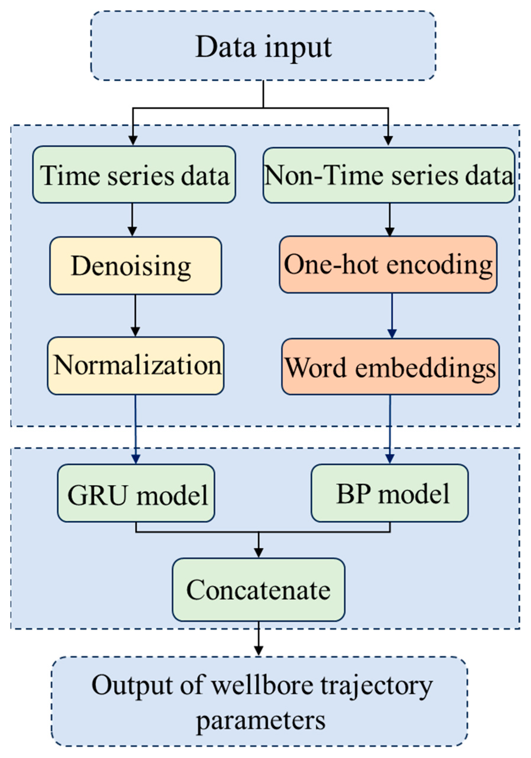
The Pi-GRU model proposed in this study differs from the traditional single-input GRU or LSTM models. It adopts a unique parallel architecture design, which can not only effectively handle the time series data provided by the downhole measurement system (such as tilt angle and azimuth angle), but also utilize BP neural networks to extract deep-level correlations in non-time series features (such as formation lithology). This design not only overcomes the problem of high computational complexity of traditional mechanical analysis methods but also makes up for the deficiency of existing data-driven models that fail to fully utilize non-temporal features. The hyperparameters were optimized by introducing orthogonal experiments, and the necessity of this parallel architecture was verified through ablation experiments, demonstrating the significant advantage of the Pi-GRU model in prediction accuracy. The overall process of this study is shown in Figure 2 below.

Figure 2.
Overall process diagram of this paper.
The rest of this paper is structured as follows. Section 2 includes a detailed introduction to data preprocessing, the procedure for constructing the Pi-GRU model, and a hyperparameter optimization scheme implemented through orthogonal experiments. Section 3 presents experiments for comparing the proposed approach with Transform, CNN-BiLSTM, and GRU models, and the necessity of stratum information is verified through ablation studies. Moreover, the generalization ability of the Pi-GRU model in different regions was validated using data from Dehong Coal Mine. Section 4 contains a summary of the research results and an overview of our future work on lightweight model variants.
2. Materials and Methods
2.1. Data Preprocessing
The performance of machine learning models is largely influenced by the quality of the input data, and this influence even surpasses the importance of the model architecture itself [16]. Therefore, constructing a high-quality dataset through appropriate data processing techniques is the key to improving the performance of a model and enhancing its generalizability.
The attitude sensor of the current mining-while-drilling measurement system adopts a combination of triaxial accelerometers and flux gates. During the movement of the drill string, the accelerometers are prone to vibration interference, and the flux gates are susceptible to instantaneous magnetic field fluctuations. A large amount of noise is contained in data collected on site. Therefore, the Kalman filtering algorithm is used to adjust the covariance matrices of the system noise and observation noise to suppress measurement noise. The Kalman filtering algorithm has been widely applied in sensor signal processing and state estimation works, and its effectiveness has been verified by the research of Li et al. [17].
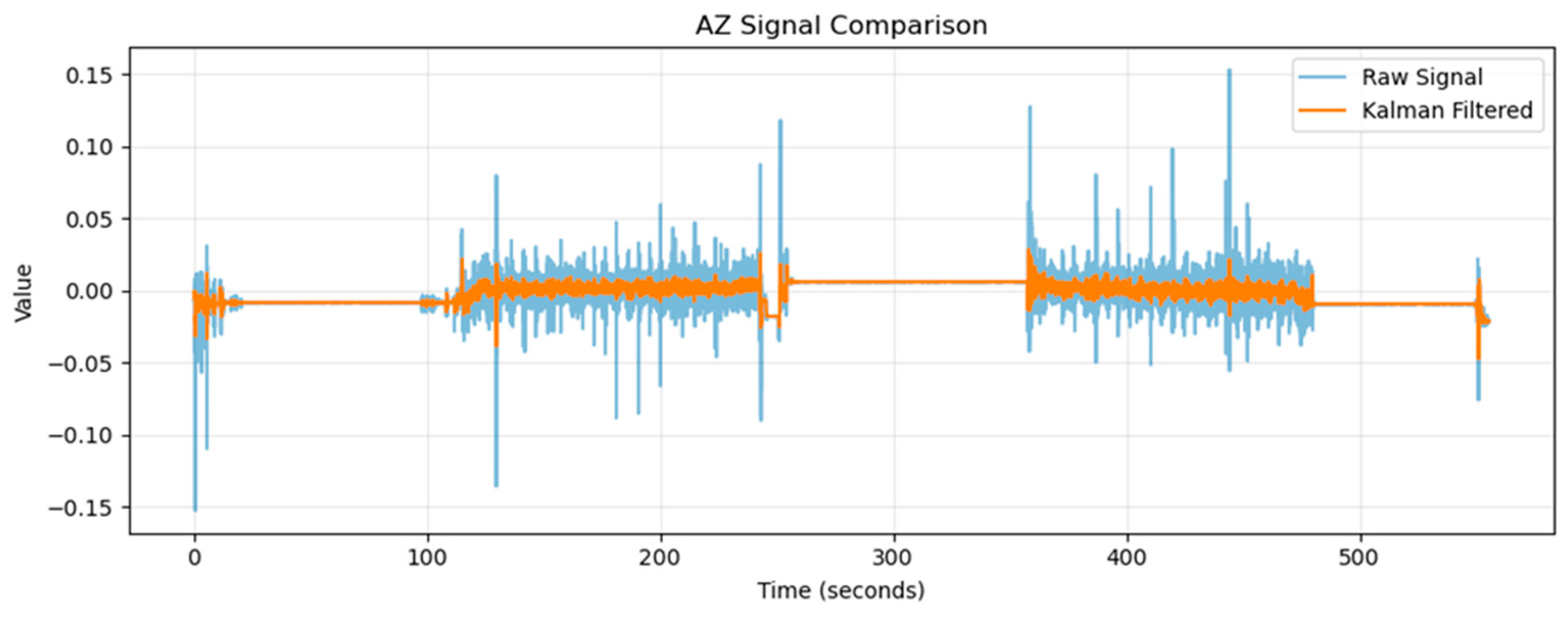
In its specific implementation, this algorithm adopts a hierarchical threshold processing strategy. When the measured values of the triaxial accelerometer or fluxgate sensor fall within the preset range, the system classifies these abnormal fluctuations in the system noise model to perform dynamic compensation. In contrast, when the sensor output values exceed the established tolerance range (such as the overlimitation of the acceleration measurement range or severe distortion of the fluxgate signal), the abnormal data elimination mechanism is triggered. This hierarchical processing method can both retain effective information and reduce the interference of transient noise in the attitude calculation system. Taking the original data AX of the accelerometer as an example, the processing results are shown in Figure 3.
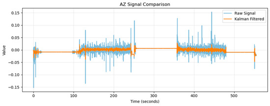
Figure 3.
Comparison between the signals AX before and after applying Kalman filtering processing.
Owing to the different orders of different input data, parameters with higher orders cause the model to pay excessive attention to them, thereby affecting the accuracy of the model. To eliminate the dimensional differences among different data features and ensure that each feature has the same importance in the model training process, the data are standardized.
Standardization is a data preprocessing technique that converts trajectory parameters such as the dip angle and azimuth into standardized features with a unified scale. Its core objective is to eliminate the unit differences in the original data, scale the data to a specific range, and ensure that different parameters are comparable during model training. During the data modeling process, the use of standardized data can highlight the degree of data dispersion, facilitate the capture of dispersed characteristics by the model, and reduce the influences of individual extreme values on the model. When the data ranges of the dip angle and azimuth are large, containing many outliers or offsets, standardization can prevent these deviations from impacting the training process by removing their means and unifying their standard deviations, enabling the model to better capture data patterns. The associated formula is as follows:
Here, represents the data value after performing standardization, represents a specific data point in the original dataset, denotes the mean of the original dataset, and signifies the standard deviation of the original dataset.
2.2. Feature Encoding for Nontime Series Data
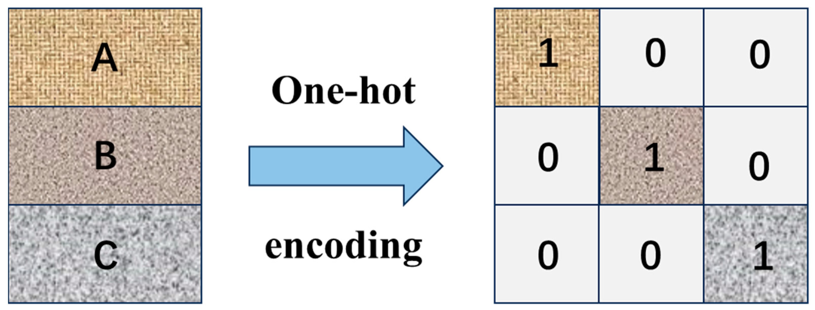
In non-time series data feature modeling tasks, the lithology types of strata and the types of drill bits are typical nonnumerical discrete variables, and they usually need to be transformed into digital data through one-hot encoding to satisfy the input requirements of machine learning models. Taking lithology classification as an example, suppose that there are different lithology categories, such as sandstone, shale, and limestone. Through one-hot encoding, each category can be converted into a unique binary vector. For example, if three lithology types are present, sandstone, shale, and limestone can be represented as [1, 0, 0], [0, 1, 0], and [0, 0, 1], respectively. This encoding method can clearly present the differences between different categories and is easy for computers to understand and process. The encoding process is shown in Figure 4.

Figure 4.
One-hot encoding process.
However, when the number of layer types is large, direct one-hot encoding results in a high-dimensional sparse matrix, which may lead to poor generalization performance and difficulty in terms of effectively learning high-dimensional sparse features. Therefore, the word embedding algorithm is used to reduce the dimensionality of the high-dimensional sparse data obtained after performing one-hot encoding. Word embedding technology has been widely applied in the field of natural language processing. It can map high-dimensional sparse word vectors to a low-dimensional continuous vector space while preserving the semantic relationships between words. In the context of stratum information processing, through word embedding technology, high-dimensional stratum information vectors can be transformed into low-dimensional dense vectors. These low-dimensional vectors can significantly reduce the data dimensionality while retaining the key stratum information features, thereby reducing the imposed computational burden and improving the training efficiency of the model.
2.3. Constructing the Pi-GRU Model
The GRU model, as a variant of a recurrent neural network (RNN), was proposed by Cho et al. [18] in 2014. Its core lies in the introduction of a gating mechanism to regulate information flows, which helps the network capture medium- and long-term dependencies. The GRU model consists of a hidden state and two gating units: a reset gate and an update gate. The reset gate is used to adjust the degree to which the current state is influenced by the previous state; the update gate controls the influences of the current input and the previous state on the present state. The structure of the GRU model is shown in Figure 5. Compared with the traditional BP neural network, the GRU performs better in terms of extracting temporal information [19]; compared with LSTM, the GRU has fewer parameters [20] and a simpler structure and is suitable for short sequences or scenarios with limited computing resources.
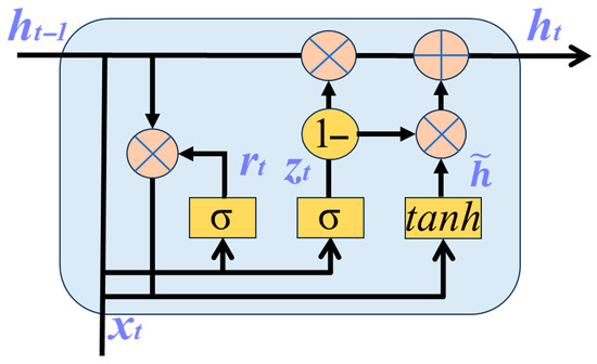
Figure 5.
Schematic diagram of the GRU structure.
Figure 5 shows the structural diagram of the GRU network. Here, represents the input vector at the current time, and is the hidden state at the previous time. represents the candidate hidden state, and represents the final hidden state. The working process of this network is as follows.
First, the reset gate determines how much information from the previous hidden state is ignored. The associated calculation formula is as follows:
Here, is the weight matrix of the reset gate, is the bias of the reset gate, and is the sigmoid activation function.
The candidate hidden state is subsequently calculated by combining the reset hidden state from the previous moment and the current input, and the calculation formula is as follows:
Here, is the weight matrix of the candidate hidden state, is the bias of the candidate hidden state, ⊙ represents the elementwise multiplication operation, and tanh is the hyperbolic tangent activation function. When ≈ 0, is ignored, the candidate state is solely determined by the current input . When ≈ 1, is retained, is jointly determined with .
Then, gate , whose function is to determine how much information acquired from the hidden state of the previous time step is retained in the current hidden state , is updated. The corresponding calculation formula is as follows:
Here, represents the weight matrix of the update gate, and represents the bias of the update gate.
Finally, by fusing the hidden state from the previous time step and the candidate hidden state of the current time step, the final hidden state is calculated. The associated calculation formula is as follows:
When is approximately 0, is approximately equal to , meaning that the old state is retained. When is approximately 1, is approximately equal to , indicating complete replacement by the new state.
The BP neural network was inspired by the human nervous system. Numerous artificial neurons (nodes) form a multilayer network through weighted connections that enable communication and interactions between neurons [21]. This neural network can be employed for training tasks such as classification, regression, and clustering. The BP network can learn and store extensive input–output pattern mappings without requiring prior knowledge about the mathematical equations describing these relationships. It adopts gradient descent as its learning rule and continuously adjusts the network weights and thresholds through BP to minimize the sum of the squared errors.
The procedure of the BP network primarily consists of two stages [22]. The first stage involves forward signal propagation: the input signals travel from the input layer, undergo processing in the hidden layer, and finally reach the output layer to produce the output result. The error between the actual output and the expected output is subsequently calculated. The second stage is backward error propagation: the error signal propagates backward from the output layer to the hidden layer and ultimately to the input layer. During this process, on the basis of the error, the weight coefficients and biases of each layer are adjusted sequentially to optimize the performance of the network, ensuring that the output aligns more closely with the expected result. The structure of the BP network is illustrated in Figure 6 below.
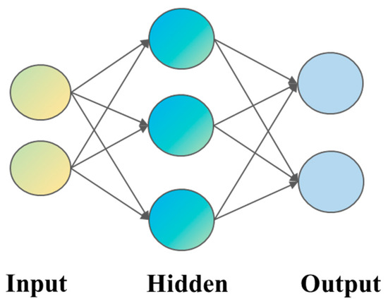
Figure 6.
BP network structure.
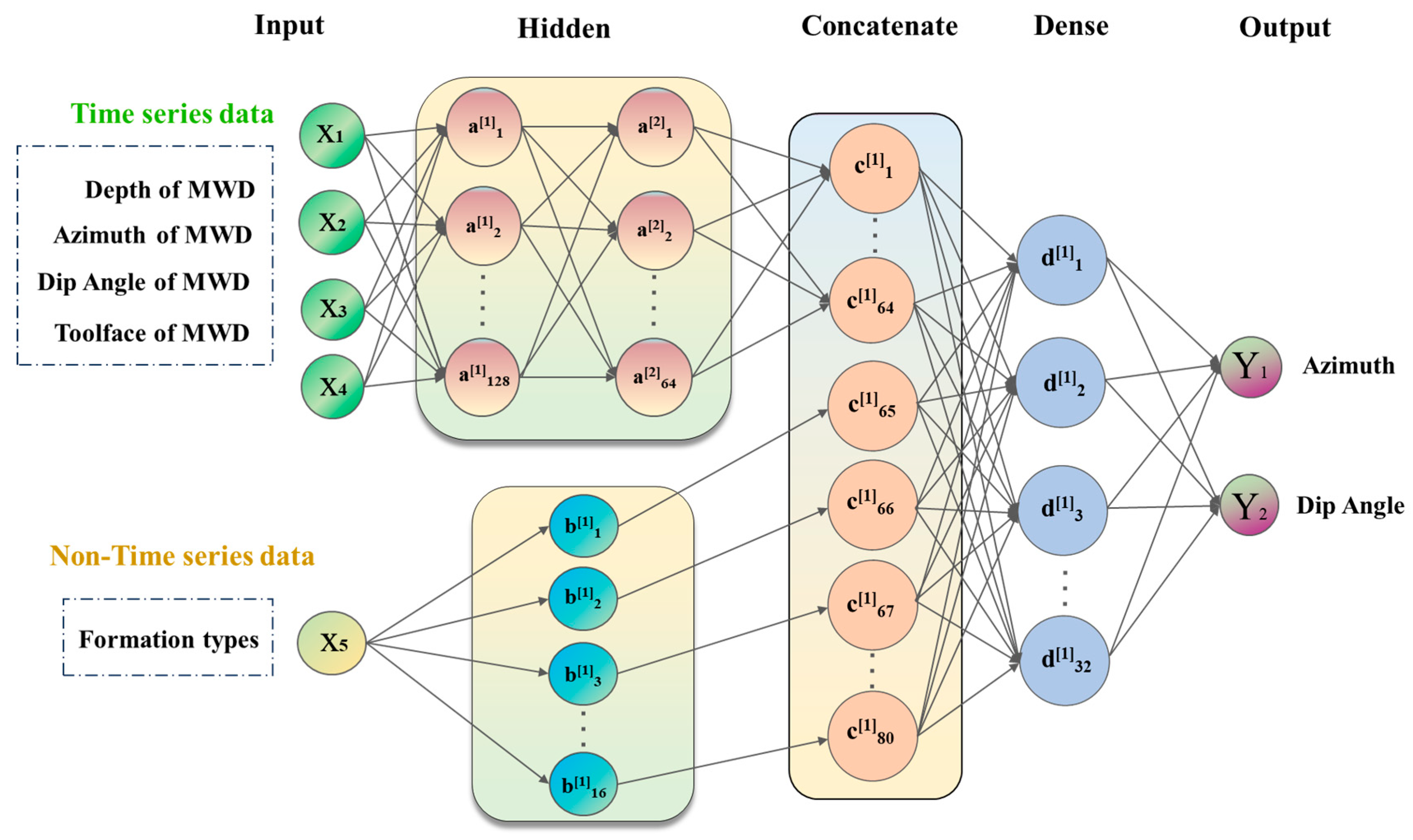
Figure 7 shows a schematic diagram of the Pi-GRU model architecture. The Pi-GRU model is constructed by combining a GRU model and a BP model in parallel, integrating the advantages of both approaches. In this model, the GRU network is responsible for processing time series data, whereas non-time series data, such as lithology types, are first processed using one-hot encoding to transform the discrete categorical information into binary vectors for category identification purposes. However, this encoding method often results in high-dimensional sparse data. To address this issue, a word embedding algorithm is further introduced to reduce the dimensionality of the data, converting them into low-dimensional dense vectors, which are then used as inputs for the BP neural network. After the GRU network and BP neural network independently complete the training process on their respective input data, the outputs acquired from both networks are fed into a fully connected layer for integration. Within the fully connected layer, the data obtained from different sources are fused, effectively consolidating the information contained in both the time series and non-time series data. Finally, the integrated data are passed to the output unit, where they undergo a series of computations and processes to generate the final predictive output.
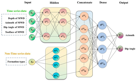
Figure 7.
Pi-GRU model structure.
This enables the Pi-GRU model to precisely predict drilling trajectory parameters and other targets.
2.4. Evaluation Metrics and Hyperparameter Optimization Scheme
To conduct an effective evaluation of the model, the mean squared error (MSE) and coefficient of determination (R2) are adopted as evaluation indicators. The formula for the MSE is as follows:
The formula for R2 is as follows:
where represents the sample quantity, is the true value of the i-th sample, is the predicted value of the i-th sample, and represents the average of all actual values . The closer R2 is to 1, the better the fit of the model is. Optimizing the hyperparameters of a model is crucial for achieving its best performance [23].
An orthogonal experiment was conducted on the optimal combination of model hyperparameters in this paper. An orthogonal experiment is an efficient experimental design method that can study the influences of multiple factors on test indicators with fewer experimental trials. The L9 (34) orthogonal table design is shown in Table 1. We trained and tested the model under various hyperparameter combinations and compared the resulting MSEs to select the hyperparameter set with the smallest MSE.

Table 1.
Orthogonal test results.
2.5. Dataset
The data used in this experiment originated from a certain mining area in Shanxi Province. In this mining area, an exploration and remediation project was implemented in the bottom plate area of the southern wing. A “comb-shaped + branch-shaped” drilling layout was adopted, and a total of 28 directional drilling holes were successfully constructed. The application of directional drilling technology in this area is relatively mature, and the accuracy and credibility of the construction data are relatively high, providing a good foundation for experimental research. In this study, the data for this experiment were sourced from the No. 2 mine field of the No. 2 drilling hole in this mining area. The drilling data within the range of 0 to 300 m were taken as the training set, as shown in Table 2, for training the neural network model. The drilling data within the range of 300 to 450 m were taken as the test set, as shown in Table 3.
Table 2.
Training dataset.
Table 3.
Test dataset.
A time series dataset was constructed using a sliding window approach, in which the window was progressively moved through the dataset. Starting from time point ‘i’, a sequence of time ‘steps’ was extracted as sequential features. The shape of the time series features was an array of sizes (steps, 4), containing the borehole depth, dip angle, azimuth angle, and tool face angle at the current time step for the previous time steps. The non-time series features were represented as a one-dimensional array of shapes (geo_encoded.shape [1]), encoding the lithology type of the prediction point using one-hot encoding. The geological characteristics of the non-time series features refer to the stratum at the prediction location, which was input into the model as prior knowledge. For example, during the drilling process, the lithological conditions at different depths were already known, so the stratum information at the prediction point could be used as part of the model input. In this case, the model could utilize the stratum information to assist in making predictions.
3. Experiments and Analysis
In this section, the optimal hyperparameter configuration obtained from the orthogonal experiment was applied to the Pi-GRU model. The test results were compared and analyzed with those of other data-driven models. Moreover, to evaluate the performance of the model in more detail, we conducted tests on the data of another mine located in the same mining area.
3.1. Experimental Design
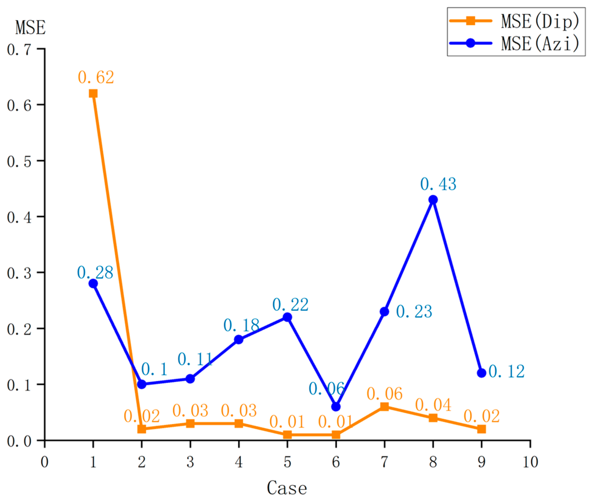
The results of the orthogonal experiment are shown in Figure 8. Among the nine experimental cases, Case 6 yielded outstanding predictive performance. At this time, the hyperparameter configuration was as follows: learning rate = 0.005, GRU neurons = 128, batch size = 16, and dropout rate = 0.3. Compared with the default learning rate (0.001), the learning rate of 0.005 accelerated the convergence speed of the model in the initial stage, and through the dynamic adjustment of the adaptive optimizer (adaptive moment estimation (Adam)), the problem of gradient oscillation was avoided. The first hidden layer, which was composed of 128 GRU neurons, significantly improved the ability of the model to capture the temporal features of the drilling trajectory. To suppress the overfitting phenomenon during the model training process, the dropout mechanism was adopted, and a dropout rate of 0.3 was set, which could effectively alleviate the risk of overfitting. During the model optimization process, the randomness of the minibatch gradient update and the random dropout strategy formed a dual random regularization effect, further enhancing the generalization ability of the model. The architecture and training process of the Pi-GRU model proposed in this paper used the TensorFlow framework, and all the codes were run in Python 3.8.

Figure 8.
Orthogonal test results.
3.2. Results
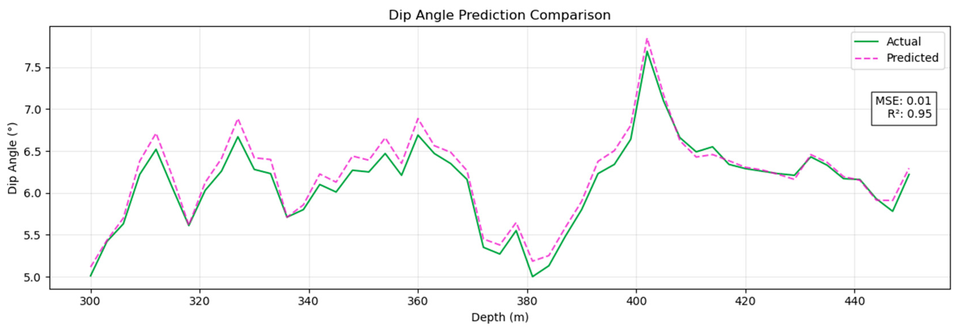
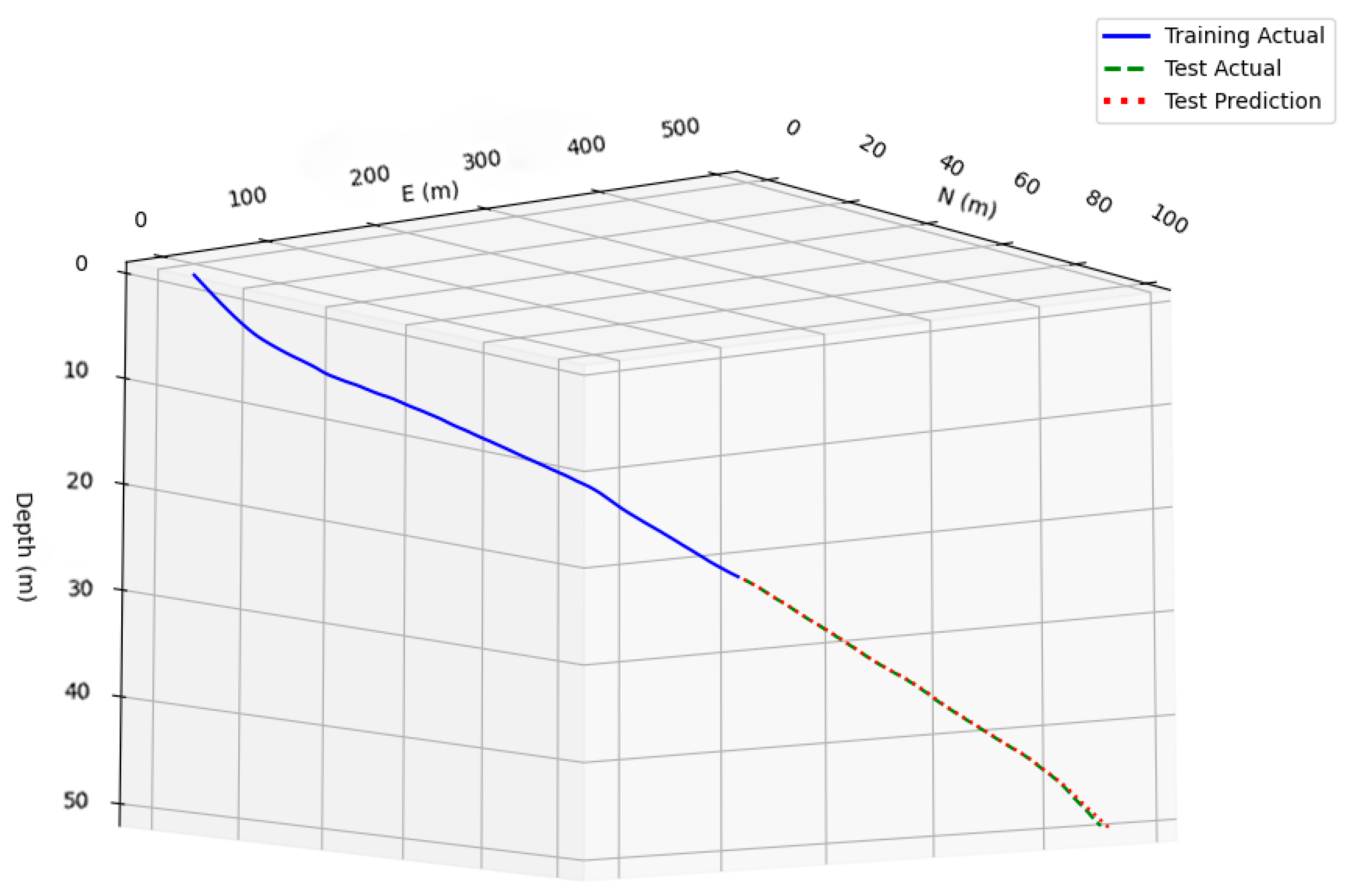
The prediction results obtained for the dip angle and azimuth angles by the Pi-GRU model are presented in Figure 9 and Figure 10, respectively. At this time, the MSE of the azimuth angle was 0.06, and the R2 was 0.93; the MSE of the dip angle was 0.01, and the R2 was 0.95. This provides strong evidence that the Pi-GRU model has high accuracy in azimuth angle and dip angle prediction tasks. The fitting effect between the predicted curve and the actual curve is excellent, and it can accurately reflect the actual change in the azimuth angle. In addition, to more intuitively display the trend of the actual wellbore trajectory and the predicted trajectory, Figure 11 shows a three-dimensional comparison diagram between these wellbore trajectories.
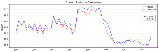
Figure 9.
Predicted azimuth results with Pi-GRU model.
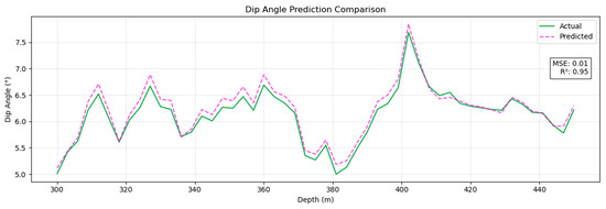
Figure 10.
Predicted dip angle results with Pi-GRU model.
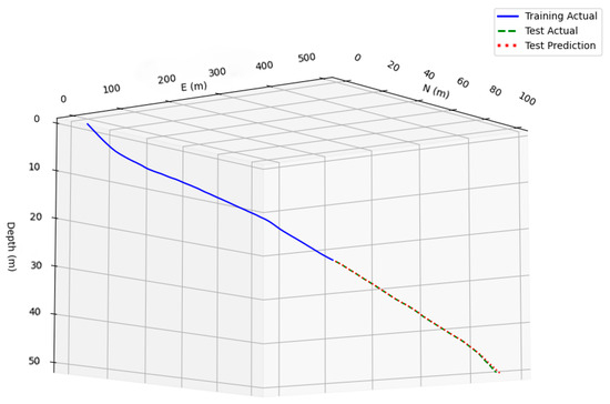
Figure 11.
Three-dimensional wellbore trajectory comparison.
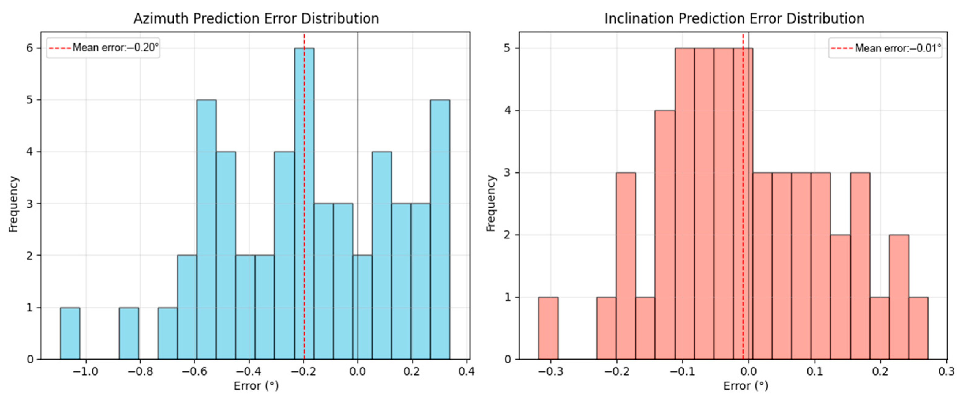
In this study, we constructed a prediction model to predict the azimuth angle and dip angle and further analyzed the prediction errors of the model. To visually display the distribution of the prediction errors, we plotted the histogram of the azimuth angle and dip angle prediction errors, as shown in Figure 12.
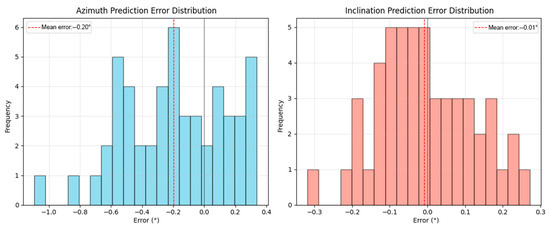
Figure 12.
Histogram of the azimuth angle and dip angle prediction errors.
From the left chart, it can be seen that the prediction error of the azimuth angle is mainly concentrated within the range of −0.4° to 0.2°. The average error is −0.20°, which indicates that the model tends to underestimate the actual azimuth angle value. Although there is a certain systematic deviation, the error distribution is relatively concentrated, indicating that the model has good stability in predicting the azimuth angle. Moreover, the narrow error range also indicates that in most cases, the model can provide predicted results that are close to the actual values.
The distribution of dip angle prediction errors is more concentrated, with most of the errors falling within the range of −0.2° to 0.2°. A significant peak appeared near 0.0° in the error value, indicating that the model’s predictions were most concentrated within this error range. The average error was −0.01°, suggesting that the model has high accuracy and stability in predicting the dip angle.
3.3. Multimodel Comparison
To comprehensively evaluate whether the Pi-GRU model outperforms other mainstream models in the current task, we designed and conducted a series of systematic comparative experiments. In the experiment, we selected five representative models as comparison baselines, namely the traditional BP (back propagation) neural network, long short-term memory network (LSTM), gated recurrent unit (GRU), and the CNN-BiLSTM model combining convolutional neural network and bidirectional long short-term memory network. And the transformer model is based on the attention mechanism. All models were trained and tested on the same dataset to ensure the fairness of the experiments and the comparability of the results. In addition, to further verify the potential of the Pi-GRU model in practical engineering applications and evaluate its advantages over traditional mechanical models, we have also incorporated the classic method of the minimum curvature method into the comparative experiment system. As a traditional method widely used in wellbore trajectory calculation, the results of the minimum curvature method have clear physical significance and engineering background. Therefore, comparing it with the prediction results of the Pi-GRU model can more intuitively reflect the improvement of the deep learning model in terms of accuracy and robustness.
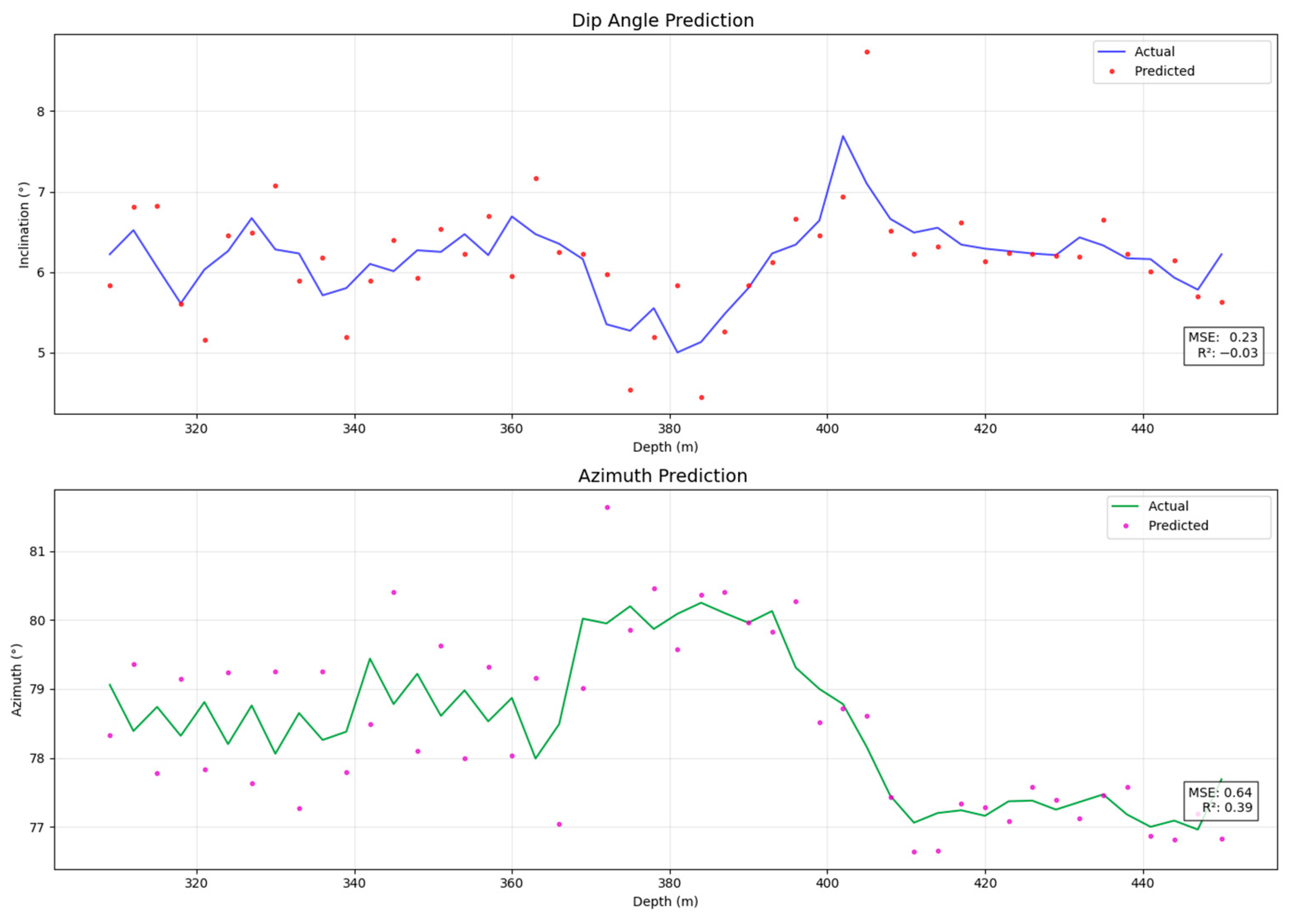
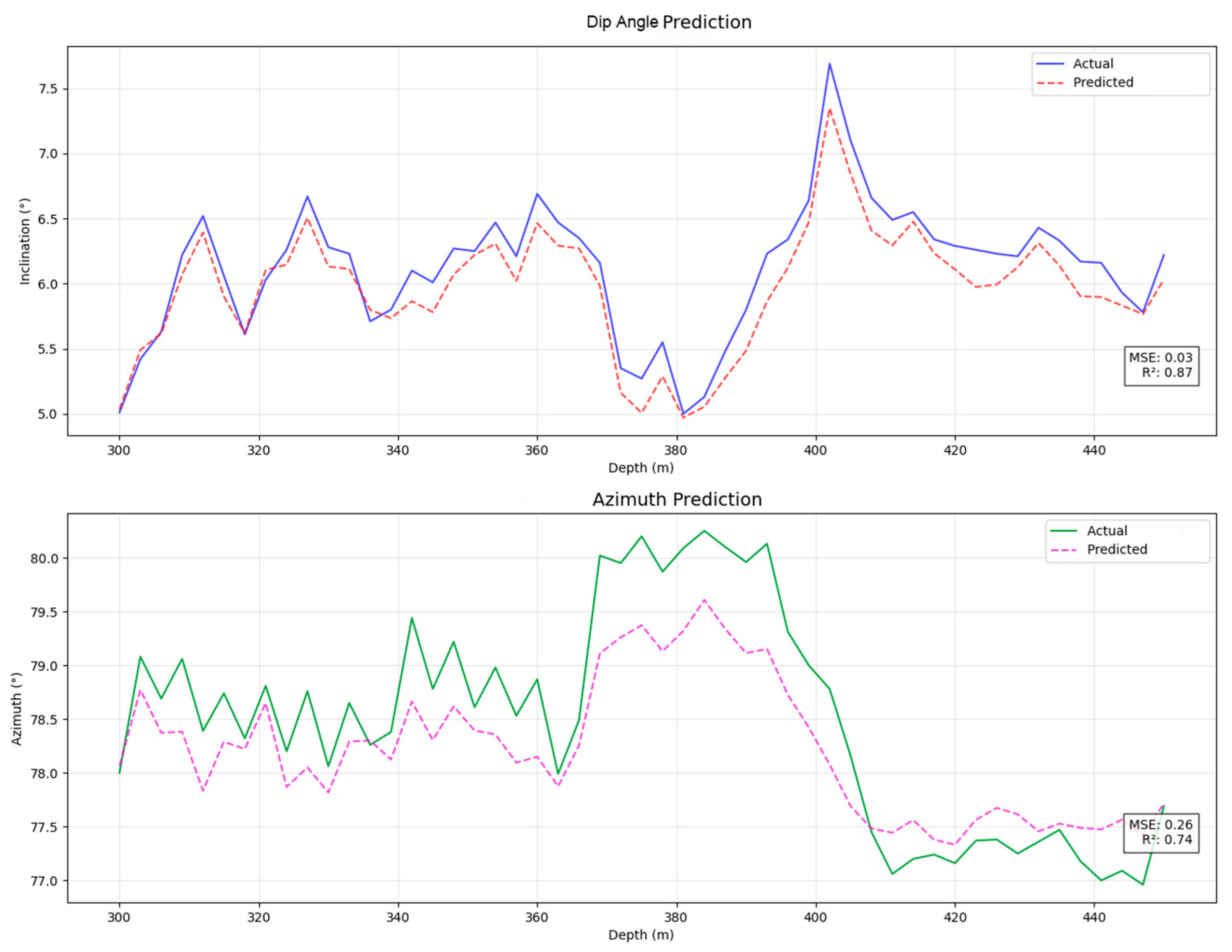
The experimental results show that the Pi-GRU model outperforms the comparison model in multiple evaluation indicators, demonstrating stronger predictive ability and generalization performance. Figure 13 and Figure 14, respectively, present the experimental results of the minimum curvature method and the CNN-BiLSTM model, serving as important references for comparison with the Pi-GRU model. By analyzing these results, we can more clearly identify the differences among various methods in terms of prediction accuracy and adaptability to complex data patterns, thereby providing strong support for subsequent model optimization and practical applications.
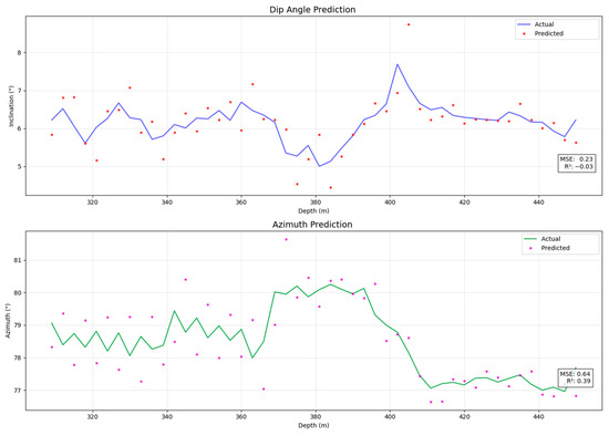
Figure 13.
The experimental results of the minimum curvature method.
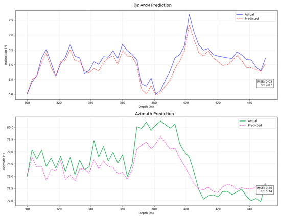
Figure 14.
Results of the CNN-BiLSTM experiment.
The comparison results are shown in Table 4. The minimum curvature method, as a representative of the traditional mechanical model, has a variance of 0.23 for the dip angle and 0.64 for the azimuth angle between the predicted value and the actual value. However, the variance of the dip angle for the Pi-GRU model is 0.01, and that of the azimuth angle is 0.06. Thus, it can be seen that the Pi-GRU model has the advantages of smaller error and higher prediction accuracy compared to the traditional mechanical model. In the comparison between the LSTM model and the Pi-GRU model, the mean square error of the dip angle decreased from 0.09 in the LSTM model to 0.01, a reduction of 88.89%, and the mean square error of the azimuth angle decreased from 0.34 to 0.06, a reduction of 82.35%. Even when facing emerging models like CNN-BiLSTM, it still shows significant advantages. Compared with the single-input model, the Pi-GRU model incorporates geological information, and its performance has been significantly improved. This finding indicates that introducing geological information enables the model to effectively reduce the trajectory drift error caused by geological condition changes (such as sudden changes in rock properties), allowing the model to more accurately capture the potential factors affecting the trajectory during the drill bit’s drilling process.
Table 4.
Results of comparative experiments involving different models.
Although the memory usage of Pi-GRU is relatively high, this resource consumption is reasonable compared with its significantly improved prediction accuracy. The training time reflects the learning efficiency and deployment feasibility of the model. The training time of Pi-GRU is 3.89 s, slightly longer than that of GRU (3.21 s) and CNN-BiLSTM (3.26 s). Considering that Pi-GRU can achieve higher prediction accuracy during the training process, its slightly longer training time is acceptable. Especially in engineering applications, the predictive performance of a model is often more crucial than its training efficiency. Therefore, Pi-GRU provides better prediction results while ensuring efficient training.
3.4. Empirical Analysis of Computational Efficiency
To comprehensively evaluate the computational complexity of the Pi-GRU model, we have made detailed records and comparisons of its inference latency, training computing power, and inference computing power on the Jetson TX2 hardware. Table 5 presents the specific performance data of the Pi-GRU model on Jetson TX2 hardware. It can be seen from the table that the Pi-GRU model performs well in terms of inference latency, which is only 0.21 ms, far below the upper limit of hardware capacity of 80 ms. This means that the Pi-GRU model can respond quickly in real-time application scenarios and meet the requirements of real-time trajectory correction. Furthermore, the training computing power and inference computing power of the Pi-GRU model are 0.29 GFLOPS and 0.093 GFLOPS, respectively, both of which are far lower than the maximum computing power of 1.3 TFLOPS of the Jetson TX2. This indicates that even on embedded devices with limited resources, the Pi-GRU model can efficiently complete training and inference tasks.
Table 5.
Evaluation of computing efficiency in engineering scenarios.
3.5. Ablation Experiment
To quantitatively evaluate the contribution of each component in the Pi-GRU model, this section designs an ablation experiment, comparing three groups of models:
- Only GRU branch: Remove the BP branch and geological feature input, and retain the temporal path;
- Only BP branch: Remove the GRU branch, and only use non-temporal features;
- Complete Pi-GRU: Include the dual-path fusion architecture.
The experimental results are shown in Figure 15. The ablation experiment confirms that in the dip angle prediction, the R2 of the only BP branch is negative (≈−2.0), indicating that its predictive ability is lower than the constant baseline model, proving that non-temporal geological features themselves do not have independent modeling capabilities. After removing the BP branch, the azimuth MSE increased by 47%, proving that geological features are indispensable for trajectory modeling. And through the dual-path fusion, the complete Pi-GRU achieved an R2 of 0.92 for the dip angle, compared to the only GRU branch (0.78), an increase of 18.7%, highlighting the adaptability breakthrough of heterogeneous features’ synergy for complex strata.
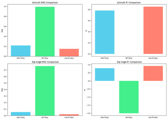
Figure 15.
Ablation experiment.
This indicates that by effectively fusing sequential and non-sequential features, Pi-GRU can ensure high prediction accuracy while avoiding complex mathematical derivation processes, providing a practical and feasible solution for real-time wellbore trajectory correction in intelligent drilling systems.
3.6. Additional Applications
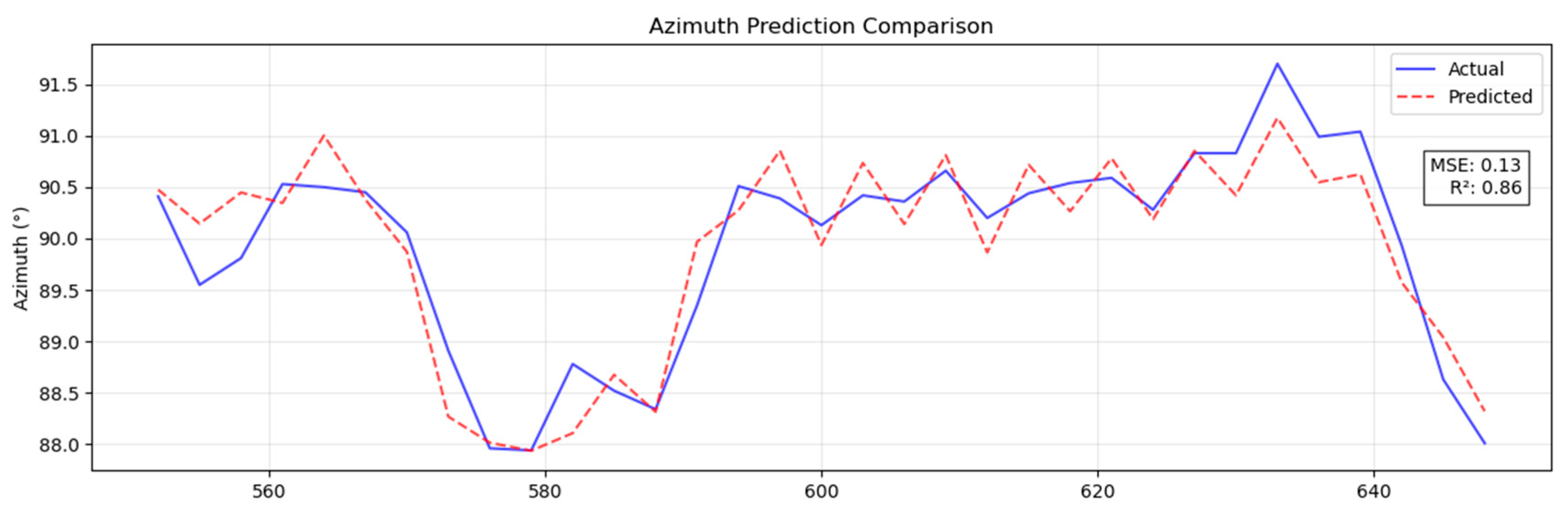
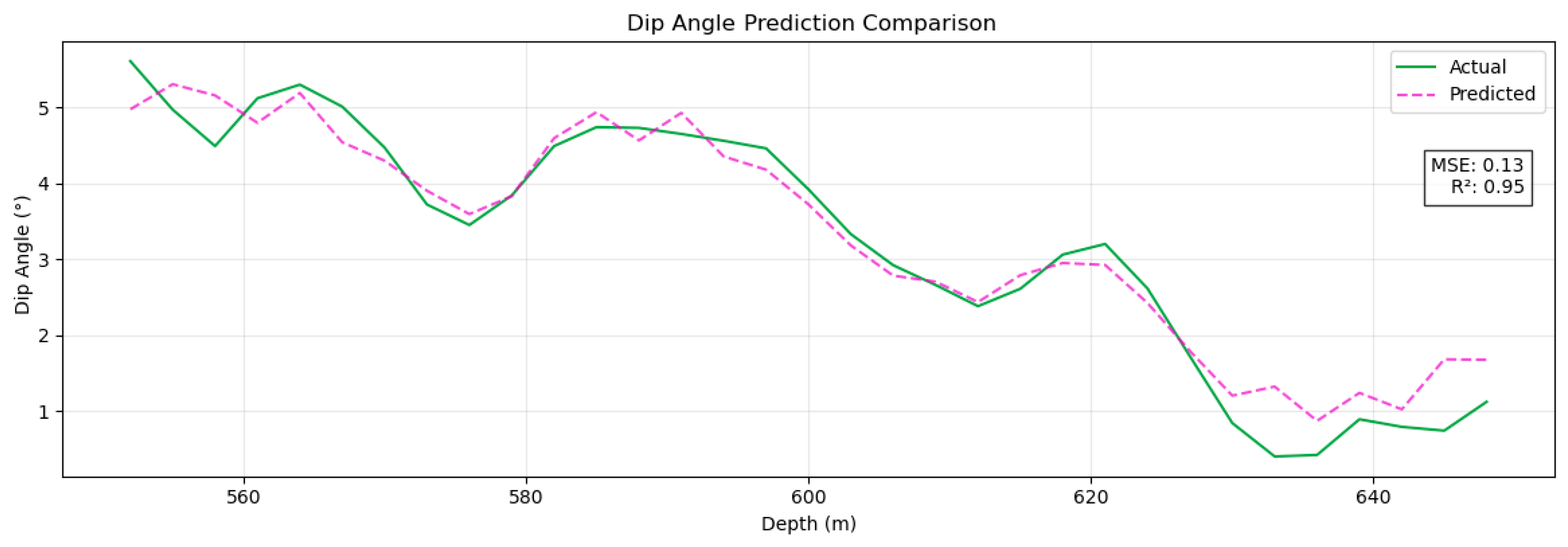
To further evaluate the generalization of the model, this study conducted cross-scenario validation based on the actual drilling data of one main shaft and two branch shafts in the Dehong Coal Mine. The test data cover the trajectories of three main and branch boreholes. Among them, the section from 114 m to 550 m is the training set (including complex formation crossing and conventional correction operations), and the target section from 550 m to 630 m is the independent test set (simulating the unknown geological conditions of the new mining area). As shown in Figure 16 and Figure 17, the model has a good ballistic prediction ability in the test section: the MSE for azimuth prediction is 0.13° (R2 = 0.86), and the MSE for tilt prediction is 0.13° (R2 = 0.95). The coefficient of determination between the dip angle prediction curve and the measured value is greater than 0.95, and the measurement accuracy reaches the sub-degree level (<0.5°, with an error ratio of 82%). The experimental results show that the Pi-GRU model can still maintain sub-degree measurement accuracy and stable generalization performance in the trajectory prediction task under unknown geological conditions, verifying its practical engineering value.
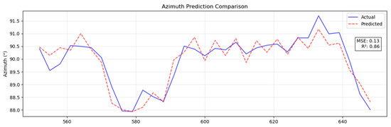
Figure 16.
Predicted azimuth results.
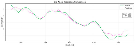
Figure 17.
Predicted dip angle results.
4. Conclusions
A Pi-GRU prediction model based on multisource data fusion, which effectively utilizes multisource data and improves the accuracy of well trajectory prediction in the near-horizontal directional drilling scenario of coal mines, is proposed in this study. A systematic verification of its performance has been conducted, and the main conclusions are as follows.
- 1.
- Innovation and effectiveness of the model
The Pi-GRU model integrates GRU and BP neural networks through a parallel architecture, achieving collaborative modeling of time series data (dip angle, azimuth angle, and tool plane angle) and non-time series data (stratum lithology). The experimental results show that the mean square errors of the azimuth and dip angle prediction results obtained on the test set of a certain mine in Shanxi Province reach 0.06° and 0.01°, respectively, which are 66.67% and 76.92% lower than those of the emerging CNN-BiLSTM model, respectively. The ablation experiment further confirmed that the deep mining of non-time series features by BP branches is the key to improving model performance. The absence of BP branches reduced the R2 of azimuth and dip angle by 8.23% and 7.6%, respectively.
- 2.
- Efficiency and practicality
Although the training time of the Pi-GRU model (3.89 s) is slightly longer than that of the single-input GRU model (2.95 s), it significantly outperforms traditional data-driven models in terms of prediction accuracy. The detailed analysis of computational efficiency indicates that the inference delay of the Pi-GRU model is only 0.21 milliseconds, and the computing power required for its training and inference is much lower than the maximum computing power of the Jetson TX2 hardware (0.29 GFLOPS and 0.093 GFLOPS, respectively). Therefore, this model not only meets the demands of real-time applications but also demonstrates strong practicality and deployability on engineering sites.
- 3.
- Generalization performance verification
To verify the generalization performance of the model, we conducted cross-scenario validation in different wells of the Dehong Coal Mine. The results show that even under unknown geological conditions, the model can still maintain high-precision predictions. This indicates that the Pi-GRU model has good stability when dealing with different stratum profiles. Although the Pi-GRU model contains a large number of parameters (approximately 90,000), by introducing orthogonal experimental design and ablation experiments to optimize hyperparameters, the risk of overfitting is effectively reduced, ensuring its good generalization ability.
In this study, the Pi-GRU model demonstrated excellent performance in wellbore trajectory prediction based on lithology and trajectory data. However, due to the availability of data, some related factors were not included.
This includes the geomechanical properties of the formation, such as tensile strength, elastic modulus, porosity, and compressibility, which have a significant impact on the interaction between the drill bit and the rock and the wellbore trajectory deviation. In addition, dynamic drilling parameters (including drill bit weight, rotational speed, torque, and drilling rate) are key indicators of downhole instability. Although these features are not available in the current dataset, in future work, it will be explored to combine them with trajectory and lithology data to enhance the model’s robustness and generalization under different drilling conditions.
Finally, as machine learning models become increasingly common in industrial applications, it is crucial to assess their vulnerability to adversarial samples. Recent studies have shown that carefully designed inputs may mislead model predictions and are not easily detected [24]. Future research will evaluate the robustness of Pi-GRU against such threats and explore strategies such as adversarial training to enhance model security.
These directions aim to further develop Pi-GRU, making it a more comprehensive, reliable, and safe tool in intelligent drilling applications.
Author Contributions
Conceptualization, H.L. and Y.H.; methodology, H.L. and Z.W.; software, H.L. and Y.H.; validation, H.L. and Z.W.; formal analysis, H.L. and Y.H.; investigation, H.L. and Y.H.; resources, Z.W.; data curation, Z.W. and Y.H.; writing—original draft preparation, H.L. and Z.W.; writing—review and editing, H.L. and Z.W.; visualization, H.L. and Z.W.; supervision, Y.H. and Z.W.; project administration, Y.H.; funding acquisition, Y.H. All authors have read and agreed to the published version of the manuscript.
Funding
This research was funded by the National Natural Science Foundation of China (grant no. 42227805).
Institutional Review Board Statement
Not applicable.
Informed Consent Statement
Not applicable.
Data Availability Statement
Data supporting the results presented in this paper are available upon reasonable request.
Conflicts of Interest
The authors declare no conflicts of interest.
References
- Hao, S.; Chu, Z.; Li, Q.; Fang, J.; Chen, L.; Liu, J. Research Status and Development Trend of Near-Bit MWD in Underground Coal Mine. Coal Geol. Explor. 2023, 51, 10–19. [Google Scholar] [CrossRef]
- Fischer, F.J. Analysis of Drillstrings in Curved Boreholes. In Proceedings of the Fall Meeting of the Society of Petroleum Engineers of AIME, Houston, TX, USA, 6–9 October 1974; p. SPE-5071-MS. [Google Scholar]
- Bengio, Y.; Simard, P.; Frasconi, P. Learning Long-Term Dependencies with Gradient Descent Is Difficult. IEEE Trans. Neural Netw. 1994, 5, 157–166. [Google Scholar] [CrossRef]
- Karlsson, H.; Brassfield, T.; Krueger, V. Performance Drilling Optimization. In Proceedings of the SPE/IADC Drilling Conference and Exhibition, New Orleans, LA, USA, 5–8 March 1985; p. SPE-13474-MS. [Google Scholar]
- Birades, M.; Fenoul, R. A Microcomputer Program for Prediction of Bottomhole Assembly Trajectory. SPE Drill. Eng. 1988, 3, 167–172. [Google Scholar] [CrossRef]
- Su, Y. A Method of Limiting Curvature and Its Applications. Acta Pet. Sin. 1997, 18, 110–114. [Google Scholar] [CrossRef]
- Eren, T.; Suicmez, V.S. Directional Drilling Positioning Calculations. J. Nat. Gas Sci. Eng. 2020, 73, 103081. [Google Scholar] [CrossRef]
- Sawaryn, S.J.; Thorogood, J.L. A Compendium of Directional Calculations Based on the Minimum Curvature Method. SPE Drill. Complet. 2005, 20, 24–36. [Google Scholar] [CrossRef]
- Liu, X.; Liu, R.; Sun, M. New Techniques Improve Well Planning and Survey Calculation for Rotary-Steerable Drilling. In Proceedings of the IADC/SPE Asia Pacific Drilling Technology Conference and Exhibition, Kuala Lumpur, Malaysia, 13–15 September 2004; p. SPE-87976-MS. [Google Scholar]
- Landar, S.; Velychkovych, A.; Mykhailiuk, V. Numerical and Analytical Models of the Mechanism of Torque and Axial Load Transmission in a Shock Absorber for Drilling Oil, Gas and Geothermal Wells. Eng. Solid Mech. 2024, 12, 207–220. [Google Scholar]
- Velichkovich, A. Design Features of Shell Springs for Drilling Dampers. Chem. Pet. Eng. 2007, 43, 458–461. [Google Scholar]
- WANG, Y.; YANG, P.; SHI, G.; SUN, Z. A Novel Method for Predicting Wellbore Trajectory Based on Support Vector Machine. Acta Pet. Sin. 2005, 26, 98. [Google Scholar]
- Yang, L.; Tian, J.; Liu, Q.; Dai, L.; Hu, Z.; Li, J. The Multidirectional Vibration and Coupling Dynamics of Drill String and Its Influence on the Wellbore Trajectory. J. Mech. Sci. Technol. 2020, 34, 2681–2692. [Google Scholar] [CrossRef]
- Huang, M.; Zhou, K.; Wang, L.; Zhou, J. Application of Long Short-Term Memory Network for Wellbore Trajectory Prediction. Pet. Sci. Technol. 2024, 42, 3185–3204. [Google Scholar] [CrossRef]
- Ye, S. Study of the Predicting Model for Directional Drilling Trajectory Controlling Based on Neural Network in Tunnel. Drill. Eng. 2024, 51, 104–110. [Google Scholar]
- Partridge, D. Network Generalization Differences Quantified. Neural Netw. 1996, 9, 263–271. [Google Scholar] [CrossRef]
- Li, Q.; Li, R.; Ji, K.; Dai, W. Kalman Filter and Its Application. In Proceedings of the 2015 8th International Conference on Intelligent Networks and Intelligent Systems (ICINIS), Tianjin, China, 1–3 November 2015; pp. 74–77. [Google Scholar]
- Cho, K.; van Merriënboer, B.; Gulcehre, C.; Bahdanau, D.; Bougares, F.; Schwenk, H.; Bengio, Y. Learning Phrase Representations Using RNN Encoder–Decoder for Statistical Machine Translation. In Proceedings of the 2014 Conference on Empirical Methods in Natural Language Processing (EMNLP), Doha, Qatar, 25–29 October 2014; pp. 1724–1734. [Google Scholar]
- Luo, F.; Liu, J.; Chen, X.; Li, S.; Yao, X.; Chen, D. Intelligent Method for Predicting Formation Pore Pressure in No. 5 Fault Zone in Shunbei Oilfield Based on BP and LSTM Neural Network. Oil Drill. Prod. Technol. 2024, 44, 506–514. [Google Scholar] [CrossRef]
- Zhang, C.; Song, X.; Liu, Z.; Ma, B.; Lv, Z.; Su, Y.; Li, G.; Zhu, Z. Real-Time and Multi-Objective Optimization of Rate-of-Penetration Using Machine Learning Methods. Geoenergy Sci. Eng. 2023, 223, 211568. [Google Scholar] [CrossRef]
- Lecun, Y. A Theoretical Framework for Back-Propagation. In Proceedings of the 1988 Connectionist Models Summer School, Pittsburgh, PA, USA, 17–26 June 1998; IEEE Computer Society Press: Los Alamitos, CA, USA, 1988; Volume 1, pp. 21–28. Available online: https://www.researchgate.net/publication/2360531_A_Theoretical_Framework_for_Back-Propagation (accessed on 24 July 2025).
- Wen, J.; Zhao, J.L.; Luo, S.W.; Han, Z. The Improvements of BP Neural Network Learning Algorithm. In Proceedings of the WCC 2000—ICSP 2000. 2000 5th International Conference on Signal Processing Proceedings. 16th World Computer Congress 2000, Beijing, China, 21–25 August 2000; Volume 3, pp. 1647–1649. [Google Scholar]
- Hutter, F.; Kotthoff, L.; Vanschoren, J. Automated Machine Learning: Methods, Systems, Challenges; Springer Nature: Berlin/Heidelberg, Germany, 2019. [Google Scholar]
- Ko, K.; Kim, S.; Kwon, H. Selective Audio Perturbations for Targeting Specific Phrases in Speech Recognition Systems. Int. J. Comput. Intell. Syst. 2025, 18, 103. [Google Scholar] [CrossRef]


Disclaimer/Publisher’s Note: The statements, opinions and data contained in all publications are solely those of the individual author(s) and contributor(s) and not of MDPI and/or the editor(s). MDPI and/or the editor(s) disclaim responsibility for any injury to people or property resulting from any ideas, methods, instructions or products referred to in the content. |
© 2025 by the authors. Licensee MDPI, Basel, Switzerland. This article is an open access article distributed under the terms and conditions of the Creative Commons Attribution (CC BY) license (https://creativecommons.org/licenses/by/4.0/).