Abstract
The widespread application of multi-agent robotic systems in domains such as agricultural collaboration and automation has accentuated the challenges faced in seeking to achieve rapid synchronization and sustain high-performance control under conditions where velocity states remain unmeasurable. To relieve these challenges, a synchronization control framework is proposed for multi-agent systems, employing non-uniform sampling communication protocols. Initially, a state-variable transformation is applied to construct a composite Lyapunov function that integrates a sampling term. An explicit relation is then derived between the communication interval and the global exponential synchronization rate, thereby establishing a theoretical foundation for the design of non-periodic sampling-based control strategies. Second, a linear-state feedback controller is introduced, which balances convergence speed with the limited frequency of information updates, ensuring asymptotic stability even under prolonged sampling intervals. Third, a velocity observer was designed based on Immersion and Invariance () theory to solve the problem of unmeasurable velocity states, ensuring the exponential convergence of the estimation error. Finally, the simulation results demonstrate that, with sampling intervals of s, the position errors of all six robots converge to below within 7 s; meanwhile, the velocity estimation errors decay to nearly zero within 7 s, confirming the effectiveness of the proposed method. The main contributions of this work can be summarized as follows: (1) a new velocity observer is tailored for discrete-time communication; (2) rigorous proof of global exponential convergence is provided via a composite Lyapunov energy function; (3) a reproducible MATLAB simulation framework is presented that enhances both the verifiability and applicability of the proposed approach.
1. Introduction
Advancements in control and optimization techniques for robotic systems have profoundly influenced science, engineering, and societal welfare, driving substantial progress in various fields. Multi-agent robotic systems not only foster the theoretical advancement of intelligent systems but also impose increasingly stringent demands on the robustness and real-time performance of practical implementations [1]. In agriculture, autonomous robots are capable of performing tasks such as sowing, monitoring, and harvesting with high precision, thereby significantly enhancing operational efficiency, reducing labor costs, and boosting overall productivity.
Early research on the stability of nonlinear dynamical systems and synchronization phenomena—rooted in Lyapunov stability theory and Poincaré’s phase space analysis [2,3] and primarily concentrating on the stability of individual systems—aims to elucidate their dynamical behavior in response to external perturbations from a qualitative perspective. In the mid-20th century, the advent of the Kalman filter and synergetics [4,5] not only represented a breakthrough in state estimation and signal fusion but also introduced effective tools for coordinated control across networked agents, marking a significant shift from single-system analysis to the cooperative control of multi-agent systems. Following the 1980s, the oscillator synchronization models proposed by Winfree and Kuramoto [6,7], inspired by physical and biological systems, uncovered the fundamental principles of self-organized synchronization by characterizing the interactions between oscillators. Concurrently, distributed control [8] and state estimation methods, exemplified by the work of Bertsekas, Tsitsiklis, and Luenberger [9,10], have expanded the theoretical foundations in this field and have provided us with systematic solutions for information transfer and feedback. In recent years, research has increasingly emphasized Immersion and Invariance (I&I) approaches, game-theoretic frameworks, and robust control strategies [11,12], focusing on adaptive compensation and global performance guarantees to relieve the effects of communication delays and systematic uncertainties common in practical applications [13]. Furthermore, studies investigating the effects of delays and non-chirality factors [14,15,16] have refined classical theories through the construction of targeted Lyapunov functions and invariant manifolds, thereby relieving design conservatism and enhancing synchronization performance in complex networked environments.
Despite the substantial advancements that have been made in robotic control, few studies have specifically solved the synchronous control of multi-agent systems under non-uniform sampling communication [17,18,19]. Conventional approaches and robust control algorithms [20,21] generally assume continuous communication or treat discrete sampling as perturbations, which impedes the establishment of stringent performance guarantees in bandwidth-limited or event-triggered networks [22], necessitating iterative trade-offs between performance and communication overheads during controller and observer tuning. To solve these limitations, this paper proposes a synchronization control framework that integrates sampling-aware stability design [23], observer synthesis, and control strategy optimization.
1.1. The Key Contributions of This Work
The key contributions of this work are summarized as follows:
- (1)
- Sampling-aware Lyapunov-based stability criterion: A novel composite Lyapunov function is constructed by incorporating sampling-interval-dependent terms [24]. Through the application of the Schur complement lemma and Jensen’s inequality, this method derives explicit sufficient conditions for global exponential synchronization, enabling accurate analysis of error convergence under discrete communication protocols.
- (2)
- Quantitative estimation of communication bounds: The proposed approach explicitly quantifies the relationship between the maximum allowable communication interval and the synchronization performance. A one-dimensional LMI-based search algorithm is introduced to compute upper bounds on sampling intervals, providing an effective tuning mechanism for discrete-time controller implementation [25].
- (3)
- Linear state feedback controller robust to non-uniform updates: A linear-state feedback controller is designed to achieve error convergence even when only intermittent information is available from neighbors. This control law effectively balances convergence speed and communication load, ensuring closed-loop asymptotic stability without requiring high-frequency updates.
- (4)
- Immersion and Invariance ()-based adaptive velocity observer: To solve unmeasurable velocity states, an observer is developed using the framework, coupled with integral compensation [26]. The observer guarantees exponential convergence of the estimation error to a predefined invariant manifold, enhancing estimation reliability under discrete sampling.
- (5)
- Implementation-friendly structure with validated performance: Compared with existing synchronization strategies, the proposed framework demonstrates superior performance through MATLAB R2022a simulations, showing improved synchronization rate, fast error convergence, and strong adaptability to communication constraints. The results confirm the method’s robustness and practicality in applications such as cooperative agricultural robotics and swarm automation.
In summary, the proposed approach overcomes traditional limitations regarding continuous communication and velocity measurability. By tightly coupling theoretical stability guarantees with implementation flexibility, this framework provides a rigorous and practical solution for multi-agent synchronization under non-uniform sampling conditions.
1.2. Compared to Other Observers
To provide a clearer comparative perspective, we provide a summary Table 1. The table categorizes representative observer methods along three dimensions: continuous/discrete, adaptive/non-adaptive, and with/without communication delay. Accordingly, the table clarifies the unique contribution of the proposed approach.

Table 1.
Comparison of common observer methodologies in nonholonomic systems.
As shown in Table 1, most existing studies concentrate on continuous-time adaptive observers, while research on their discrete-time counterparts is still limited, particularly under parameter uncertainties and communication constraints. The proposed discrete-time adaptive observer not only solves the velocity estimation problem in nonholonomic systems, but also extends naturally to cases with communication delays, thereby filling an important research gap.
1.3. Structure of the Article
To facilitate the reader’s understanding of the overall structure, the remainder of this article is organized as follows:
- 1.
- Section 2—Preliminaries: This section introduces the system modeling and preliminaries, including the dynamics of nonholonomic mobile robots and necessary definitions.
- 2.
- Section 3—Stability Criterion Conditions: This section presents the stability criterion conditions under sampled data communications.
- 3.
- Section 4—State Feedback Controller: This section develops a state feedback controller and provides the corresponding stability proof.
- 4.
- Section 5—An I&I Velocity Observer: This section proposes an adaptive velocity observer based on the Immersion and Invariance (I&I) approach, and analyzes its convergence properties.
- 5.
- Section 6—Simulation: This section demonstrates the effectiveness and superiority of the proposed methods through simulation results.
- 6.
- Section 7—Discussion: A thorough discussion was conducted, comparing the proposed approach with other representative advanced methods.
- 7.
- Section 8—Conclusions: This section concludes the paper and outlines directions for future research.
2. Preliminaries
The following is a model construction of the system and the definition and lemma that need to be used:
2.1. System Modeling and State Description
In order to explicitly establish the connection between the observer design and the actual dynamics of nonholonomic mobile robots, we first consider the standard kinematic and dynamic model of a differential-drive robot. For each robot, i, let denote the generalized coordinates, where is the position and is the heading angle. The control inputs are the linear velocity, , and the angular velocity, . The kinematic equations are given by
Define the generalized velocity vector . The dynamics can be written in compact form as
where
Define the world-frame generalized velocity
From trigonometric kinematics to a lifted second-order form, differentiating gives
Since with , one obtains
As the columns of are orthonormal, it holds that
Thus, designing a velocity observer is equivalent to estimating and then recovering via (7).
We postulate the following standard assumption used in mobile robot cascade designs.
Assumption 1
(Inner-loop acceleration servo). There exists a low-level velocity controller that can track any piecewise continuous command, , sufficiently fast (relative to the observer dynamics). In particular, we can command
where are constant design matrices.
Remark 1.
In the original nonholonomic mechanics, the corresponding matrices would be state-dependent. Here, by invoking the inner-loop acceleration servo and feedback cancellation in (8), the trigonometric state dependence is compensated, and the outer-loop model seen from the observer reduces exactly to the constant matrix form with the designer-chosen .
Substituting (8) into (5) gives
according to Remark 2 and together with from (4), we obtain the following exact second-order form:
Equation (9) can be rewritten as
In the networked/controlled setting, the outer-loop couplings and inputs are added to the acceleration channel (the -equation). Let
and define the injection matrix
Then, the closed-loop system is
Expanding Equation (11) yields [27]
where , A is the system matrix. , is the communication moment that satisfies
where . is the state vector of node i. c is the connection strength and is the connection configuration matrix. is an inner connectivity matrix with appropriate dimensions. is the control gain matrix, and u is the external control input. In addition, , G, and are constant matrices, while the distance between any two consecutive communication moments referred to in this paper is assumed to be bounded, i.e., it is assumed that
where , h is the permitted communication interval and is a positive scalar.
Let
Therefore, the system (12) can be re-expressed as
where .
Definition 1.
In this paper, is defined as the connection configuration matrix; if there is a link between node i and node j, then ; otherwise, . The diagonal elements are defined by
This construction is exactly the definition of the graph Laplacian matrix. Consequently, G always satisfies the zero row sum property. If the communication graph is undirected and connected, then G possesses the following well-known properties:
- 1.
- G is symmetric;
- 2.
- (positive semi-definite);
- 3.
- , i.e., the zero eigenvalue has multiplicity one.
Therefore, in the subsequent stability analysis, G is treated as the Laplacian matrix of an undirected connected graph, and its spectral properties are explicitly utilized.
Remark 2.
Equations (1)–(9) make explicit the trigonometric nonholonomic structure via ; meanwhile, under Assumption 1, the closed-loop (outer-loop) model exactly matches the constant matrix abstract system in (12). The matrices are design constants to shape the observer error dynamics; they are not robot physical constants.
2.2. Definition and Conditions for Global Exponential Synchronization
Definition 2
([28]). The system (12) is said to be globally exponentially synchronized if there exist constants α and ; such that, for any initial values (i = 1, 2, …, N) and sufficient large ,
where .
It should be clarified that this definition does not imply that all robots physically coincide at the same spatial point. Instead, it means that the relative state errors among robots exponentially converge to zero, i.e., their trajectories asymptotically align or follow a common reference pattern. This distinction is crucial in multi-agent systems, where synchronization refers to consistency in states or behaviors rather than literal positional overlap.
Lemma 1
([29]). is a matrix that satisfies the same sum for each row. The following equation holds:
where , .
2.3. Transformation of the Multi-Agent Synchronization Problem
To justify Lemma 1 and the synchronization of the system, auxiliary variables are introduced to describe the state differences between nodes, such that
Assuming that there exists a transformation matrix, M, such that , the definition of Lemma 1 can be justified by using the coupling matrix G and the property that each row sum is equal.
Based on Lemma 1, the system (13) can be converted via to
where , , thus reformulating the multi-agent synchronization problem as a convergence analysis of .
3. Stability Criterion Conditions
Under non-fixed sampling communication, the system state is updated only at discrete instants, and discontinuous updating of state information poses a potential risk to the synchronization stability of the system. Consequently, stability analyses must account for the dynamic discontinuities caused by discrete communications. This necessitates the construction of an energy function that accurately captures error evolution and clarifies the impact of the sampling period on error convergence rates. Based on the previously established error system model, this paper embeds the communication interval constraints into time-varying parameters, and embeds these into the design of the energy function by constructing the composite Lyapunov function; at the same time, it establishes the explicit quantitative relationship between error decay rates and the maximum communication interval by combining the Schur complement theorem and Jensen’s inequality to rigorously prove the sufficient condition of the global exponential synchronization. This approach transcends the limitations of the traditional continuous-time stability framework and provides a theoretical guarantee for the stability verification of multi-agent robotic systems under asynchronous communication.
3.1. Design of Lyapunov Functions
In order to prove that the system can achieve global exponential synchronization, this paper uses the Lyapunov method to construct composite Lyapunov functions. For the system (16), consider the following Lyapunov function:
where .
is an appropriate positive matrix to measure the energy of the current synchronization error.
this term captures the energy variation induced by dynamic changes during a continuous communication interval, using an integral formulation to account for the cumulative effect of error evolution.
where is a matrix designed to compensate for the coupling effect between the error terms.
It is noted that vanishes before and so does after , such that we get . Hence, is continuous.
3.2. Lyapunov Function Stability Analysis
According to the design of the Lyapunov function, it can be obtained based on the Schur complement theorem
where
For the results, using Jensen’s inequality, the following can be obtained:
where , , , and .
From the results, it can be deduced that
For a given scalar, h, if there exist matrices , , X and are free matrices without symmetry constraints, , and a diagonal matrix , then we have
where , and using the Schur complement again, the following can be obtained:
Thus, it is always possible to find a small enough scalar, , for which there exists . Then, you can get
Now, we get , an available Lyapunov function for system (16) from the definition (17). Then, we obtain the following derivative equality and inequality:
where , .
Applying the free weighted matrix method of [21] for any matrix H with the appropriate dimensions, we will obtain the following inequality:
where .
Therefore, according to the above equation as well as , , and , the following can be obtained:
where
and
Remark 3
([27]). To obtain the allowable communication interval, h—and therefore ensuring the globally exponential synchronization of the system (12)—the following one-dimensional search algorithm could be applied:
Step 3: If LMIs (22) and LMIs (23) are feasible, then let , and go back to Step 2. Otherwise, go to Step 4.
Step 4: Output is the allowable communication interval, h, ensuring the globally exponential synchronization of the system (12).
LMIs (22) and LMIs (23) are treated as a single feasibility problem with decision variables P, , , , X, , , and and parameters A, Γ, G, and h. They can be solved in MATLAB.
It should be noted that the relationship between the sampling step, h, and the convergence rate is crucial for ensuring global exponential synchronization. We explicitly define the maximum allowable communication step, , which ensures synchronization within a given time frame. If the sampling step, h, exceeds , then the system may experience slower convergence rates. The maximum allowable step, , is derived from the feasibility conditions defined by LMIs, ensuring that synchronization can still occur without exceeding the stability bounds. Thus, for synchronization to occur effectively, the sampling step must satisfy , which directly influences the convergence rate.
Remark 4.
It should be pointed out that, when the algorithm proposed in Remark 3 is applied, a more accurate allowable communication interval, h, can be obtained by choosing the smaller initial, h, and . For this example, we choose initial and , which is enough to ensure that the allowable communication intervals, h, show effectiveness and an advantage over adaptive control algorithms.
Because of the matrix in (31), and because there exists a scalar , such that , the following can be introduced:
According to (17), it can be concluded that
where , .
It follows from this that
where .
From (23), there exists a scalar , such that the following equation holds:
where .
In addition, there exists another scalar , thus
Making sufficiently small can allow us to obtain
So
Let , integrating over (35), yield
At the same time, combining (25) yields
The results demonstrate that the proposed method establishes synchronization for non-completely constrained dynamical systems, guarantees exponential convergence of the system state, and provides a theoretical foundation for subsequent control design.
Remark 5.
Compared with the existing synchronization results in the literature [20,21,27,29], the proposed method presents the following key distinctions and contributions:
- (1)
- Discrete-time synchronization without approximation: Most traditional synchronization methods assume either continuous-time communication or treat discrete sampling as small perturbations, which weakens stability guarantees. In contrast, our method directly incorporates the discrete-time sampling mechanism into the stability criterion without approximation, leading to rigorous exponential convergence conditions under non-uniform sampling.
- (2)
- Composite Lyapunov function design specific to discrete communication: Instead of using classical energy-based Lyapunov designs, we construct a composite Lyapunov function that explicitly integrates sampling intervals as time-varying parameters. This allows the derivation of explicit upper bounds for communication delays via LMIs, which is not solved in prior works.
- (3)
- Integration of velocity observer into synchronization framework: Existing works often assume full state availability or rely on high-gain observers that may be sensitive to noise or sampling mismatch. This paper introduces a low-complexity I&I-based adaptive observer that guarantees exponential convergence of the velocity estimation error, even under communication constraints.
- (4)
- Improved communication tolerance, as demonstrated by the simulation: The simulation results confirm that the proposed method permits larger allowable communication intervals than state-of-the-art adaptive control strategies, while still achieving global exponential synchronization—highlighting the practical benefits in bandwidth-limited or event-driven multi-agent systems.
These improvements extend the scope and applicability of synchronization control strategies, offering a unified and implementable solution suitable for multi-agent systems operating under asynchronous, sampled-data communications [30].
4. State Feedback Controller
In multi-agent robotic systems, achieving state synchronization among nodes requires the design of an appropriate feedback controller. However, under non-uniform sampling communication, the controller cannot continuously access up-to-date state information from all neighboring nodes, imposing stringent requirements on closed-loop performances. Given the continuous linear dynamics system and the partition of states into measurable positions and unmeasurable velocities, a control strategy must be devised to ensure asymptotic convergence of the error dynamics under limited information updates. Based on the stability analysis, a linear-state feedback controller is constructed and the gain matrix is determined, achieving the closed-loop regulation of the error state, so as to ensure that the closed-loop error system is asymptotically stable under the known communication structure and the bounded sampling period.
4.1. Systematic Error Dynamics Model Redefinition
Design a state feedback controller based on the system (16): by controlling the inputs, u, we can enable the system to make the state of node converge to a reference trajectory .
Define the state error as
The part of the stability criterion used to describe the interactions is now redefined as an external input in order to be more flexible in dealing with non-eliminable interactions in real systems, i.e., letting denote the interaction dynamics between the nodes. The error dynamics system of the state feedback controller is
where are the sub-matrices of the system matrix , captures the coupling between position and velocity, and represents the linear dynamics of velocity; c is a connection strength parameter measuring the influence of neighbor interactions in the error dynamics; is an inner connectivity matrix that defines the coupling structure among neighboring agents; is the elements of the communication topology matrix, . If node i and j are connected, then ; otherwise, and ; are the positive definite diagonal feedback gain matrices for position and velocity, respectively, ensuring the asymptotic stability of the error dynamics; K is a control gain matrix used in the compensatory term to balance the control input and system dynamics; is a derivative of the desired velocity trajectory, included to compensate for the reference signal dynamics.
The main task of designing a state feedback controller is to design a control input, u, such that the error asymptotically converges.
where is the feedback gain matrix, and denotes the neighbor velocity estimation signal used by the controller, and the compensation term is used to handle the interaction dynamics and reference trajectories of the system.
Substituting this control law into the system, the error dynamic equation becomes
4.2. Compensatory Term Design
To counteract the interactive dynamics of the system and the non-chiral terms of the desired trajectory, the following compensation term is chosen [31]:
Substituting into the error dynamic equation gives
Collate error dynamics system can be obtained
4.3. Stability Analysis of Closed-Loop Systems
Represent the error system in state-space form
The eigenvalue analysis is performed and the system matrix is designed as
So, the characteristic equation is
The asymptotic stabilization of the error system can be ensured by choosing ; makes the closed-loop system have negative real part eigenvalues.
4.4. The Final Form of the Controller
The control law of the state feedback controller is
where is a scalar design parameter.
4.5. Parameter Tuning Procedure
To ensure the closed-loop stability of the state feedback controller under discrete communication constraints, the feedback gain matrices should be tuned according to the following steps:
Step 1—system identification: determine the system matrices, , and the communication topology, , to establish the error dynamics in (42).
Step 2—eigenvalue analysis: analyze the closed-loop characteristic equation
and ensure that all eigenvalues have negative real parts for asymptotic stability.
Step 3—initial gain selection: Choose diagonal matrices as initial feedback gains, and verify the feasibility of the stability conditions using the LMIs introduced in Section 3. If not satisfied, gradually increase the gain values to improve convergence speed.
Step 4—compensation parameter: Introduce the compensation scalar , which balances the interaction term and the reference trajectory. A larger j accelerates convergence but may increase control input oscillations; thus, it should be carefully tuned.
Step 5—simulation-based refinement: Conduct numerical simulations (e.g., in MATLAB) under various parameter settings to evaluate error convergence speed and control effort. Select the parameter set that achieves the best trade-off between convergence rate and control input magnitude.
Following this procedure provides a systematic way to select gain parameters that guarantee asymptotic stability while maintaining robustness under limited communication updates.
4.6. Lyapunov Stability Proof
First, define an appropriate Lyapunov function:
Its time derivative is
Substituting the error dynamical system gives
We can then obtain, using the Cauchy-Schwarz and Young inequalities,
Organize this as
when , , , the system is asymptotically stable.
Therefore, the state feedback controller is
It is proved by Lyapunov stability that the controller ensures that the state of the system converges to the target trajectory.
Remark 6.
It should be emphasized that, although the neighborhood velocity, , is unmeasurable in practice, the controller does not directly use this unavailable signal, but instead uses .
5. An I&I Velocity Observer
In practice, continuously measuring all state variables (particularly linear and angular velocities) is often infeasible; hence, unmeasurable states must be estimated and compensated for by using an observer. Given the system’s continuous linear dynamics and event-triggered discrete communications among agents [32], in order to avoid increasing the communication overheads, the observer must operate stably in continuous time with a simple architecture and guaranteed convergence. Accordingly, this paper employs the Immersion and Invariance (I&I) methodology [11,33] to design a velocity observer. The state is partitioned into measurable (position) and unmeasurable (velocity) components, an error dynamics model is formulated, and the observer gains with integral compensation are designed to ensure exponential error convergence in the absence of disturbances. The I&I-based observer guarantees finite-time convergence of estimation errors to the prescribed invariant manifold, effectively mitigating accuracy degradation due to discrete communication and unmeasurable states, and providing a foundation for the practical implementation of the closed-loop control system.
5.1. State Decomposition and Dynamic Equation Definition
Describe the system (12) as
where .
is the trajectory of the system in the ideal state; let
Assume that the system matrix , where I is a unit matrix. Therefore, the dynamical equations of the original system can be rewritten as [31]
The dynamic equation for the velocity observer is
5.2. Definition of Observation Error and Error Dynamic Equation
Let , be the observation errors of the system in position and velocity, respectively:
According to the definition of observation error, let the error dynamic equation be
Since neighbor velocities are unmeasurable, all terms involving in the controller and observer should be interpreted as their estimated values, . The observer guarantees exponential convergence of the estimation error, so this substitution does not compromise stability under sampled communication.
Remark 7.
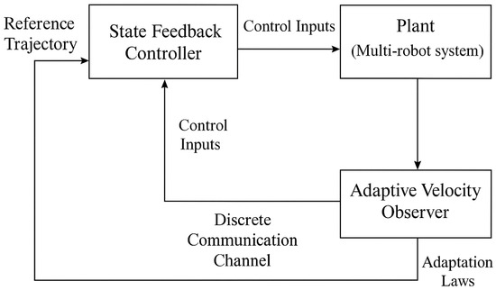
To provide a clearer understanding of the interaction among different modules, a block diagram of the proposed control framework and adaptive velocity observer is given in Figure 1. As shown, the plant (multi-robot system) generates unmeasurable velocity states, which are transmitted through the discrete-time communication channel. These signals are processed by the Immersion and Invariance ()-based adaptive observer, where adaptation laws ensure exponential convergence of the estimation errors. The estimated velocities are then supplied to the linear-state feedback controller, which combines them with the reference trajectory to produce control inputs for the plant. This closed-loop structure highlights the coupling between the plant, observer, adaptation laws, controller, and discrete communication.
Figure 1.
Block diagram of the proposed control system and adaptive observer structure.
5.3. Design of Invariant Manifolds
Design an invariant manifold [11] and define it as
The estimated state of the observer is identical to the true state if the error converges exactly on the invariant manifold.
5.4. Select a Lyapunov Function
Choose an appropriate Lyapunov function
where P is a positive matrix that weighs the rate of convergence of , , is the total error vector.
5.5. Design the Gain Matrix L
To design the gain matrix, L, L needs to satisfy the following conditions [11]:
- 1.
- must satisfy convergence;
- 2.
- must remain stable in the closed-loop system.
Let
5.6. Proof of Convergence of the Error Dynamic Equations
Bringing (63) into the error dynamic equation yields
It can be deduced that
5.7. Proof of Convergence of Estimator Errors
Firstly, the estimator error is defined as
The speed consists of a proportional part and an integral part
Thus, the dynamic behavior of is
Let , , collation is available
From the above equation, it can be deduced that
Organized into matrix form,
where .
One of its solutions is
where . Therefore, the velocity estimation exponentially converges to zero.
So, the velocity observer is
This velocity observer enables the system to estimate the velocity quickly and stably, providing powerful observation support for the cooperative control of multi-agent robotic systems.
Remark 8
(Effect of non-uniform sampling.). In practical systems, sampling intervals are often not strictly uniform.
Let the sampling instants be with intervals . In this case, the observer error dynamics can be expressed as , where , is the state transition matrix depending on the sampling interval, and denotes the perturbation caused by the non-uniformity.
By Lyapunov analysis, as long as is upper-bounded by , we have , and the perturbation term remains bounded. Thus, the overall estimation error system still guarantees exponential convergence. The difference is that the convergence rate may be limited by .
Therefore, the main results in this paper remain valid under non-uniform sampling, with the convergence rate potentially reduced.
5.8. Closed-Loop Stability with Integrated Controller and Observer Under Non-Uniform Sampling
For any neighbor, j, and any , define the controller-available neighbor velocity as the sampled-and-held observer output:
where is the local observer estimate. Let with , where is given by the feasible LMIs in Section 3 together with the one-dimensional search in Remark 3.
5.8.1. Sampling-Induced Injection
At each sampling instant, , the mismatch equals the observer’s velocity error:
5.8.2. Closed-Loop Error Dynamics with Injection
Let denote the regulation error as in Section 4 and the observer error as in Section 5. With used in the controller, the z-dynamics over can be written as
where ℑ is the nominal exponentially stable matrix from Section 4 (full-state case) and ♭ is a constant matrix compatible with the coupling channel. There exists , such that .
5.8.3. Composite Lyapunov Function and Key Bounds
Select the Lyapunov function (47) from Section 4 and the Lyapunov function (60) from Section 5. Define the composite function with a new scalar weight
There exist and , such that
Because the e-system is exponentially stable and , there exist equivalence constants and , such that
Similarly, let satisfy . Then, for any , Young’s inequality yields
Therefore,
Define
Choose and . Then, there exists , e.g., , such that
Hence, under the admissible non-uniform sampling bound, , obtained from the LMIs and Remark 3 in Section 3, the closed-loop system using remains globally exponentially stable.
Remark 9.
Although synchronization control and observer design for multi-agent systems have been extensively studied, existing results still exhibit several limitations, particularly when applied to systems with discrete-time communication and unmeasurable velocity states. In comparison, the proposed framework offers the following technical improvements:
- (1)
- Lyapunov-based synchronization criterion tailored to discrete communication: While prior works [20,29] mainly rely on continuous-time Lyapunov approaches or treat discrete communication as small perturbations, this paper constructs a composite Lyapunov function that explicitly incorporates sampling intervals, enabling rigorous global exponential convergence analysis under asynchronous updates. Unlike [27], which uses constant-step sampling, our approach supports non-uniform sampling intervals without losing generality.
- (2)
- LMI-based estimation of maximum allowable communication interval: Rather than assuming the existence of suitable sampling rates, we propose a constructive LMI-based algorithm to compute the maximum allowable sampling interval that guarantees synchronization. This quantitative criterion allows adaptive trade-offs between synchronization speed and communication cost, which are not solved in most existing synchronization methods.
- (3)
- Integration of an velocity observer for unmeasurable states: Most synchronization frameworks assume full-state availability or use high-gain observers sensitive to sampling noise. In contrast, this paper integrates a low-complexity observer into the synchronization framework, designed specifically for systems with unmeasurable velocity. The observer ensures exponential convergence of velocity estimation, which improves robustness in discrete settings.
- (4)
- Practical state feedback controller design under discrete sampling: The proposed linear-state feedback controller is designed with consideration of limited update frequency. Compared with adaptive or nonlinear control laws used in [21], our controller maintains simplicity while ensuring closed-loop stability under sparse communication, making it more suitable for real-world deployment.
- (5)
- Superior synchronization performance demonstrated via simulation: The proposed method allows larger communication intervals while maintaining exponential synchronization, outperforming existing adaptive control benchmarks. Simulation results confirm faster error decay and improved convergence compared to prior algorithms, particularly under low communication frequency and limited observability.
In summary, the technical contributions of this paper extend beyond existing literature by bridging the gap between theoretical synchronization criteria and practical implementation under discrete-time communication and velocity uncertainty.
6. Simulation
In this section, simulation experiments under a non-uniform sampling communication mechanism are conducted in Matlab to validate the proposed controller and observer. The closed-loop dynamics are integrated with a fixed-step Euler method (step size s) over a 15 s horizon, and rng(1) is used to ensure reproducibility. Neighbor velocities are available only at sampling instants and are held constant in between, which captures the effect of discrete communications.
Six agents are considered. Each agent consists of a position vector, , and a generalized velocity, , giving six states per agent. The desired equilibrium is set to and . The state feedback gains are chosen as and , with a compensation factor . The observer parameters are and . The plant follows a second-order model with , , , , and coupling gain . The non-uniform sampling interval is s. The initial conditions are
Observer initials are ( is a small disturbance with zero mean and a standard deviation of approximately 0.025), , and . To assess stability, we log the composite energy , together with per-agent position norms .
The simulation results validate the effectiveness of the controller and observer from multiple perspectives, and the details are as follows:
- 1.
- By applying the algorithms described in Remark 3, with and , Table 2 presents the allowable communication intervals-h, corresponding to different connection strengths-c, under both the algorithms proposed in this paper and the adaptive control algorithm.
Table 2. Allowable communication interval, h.
- 2.
- In the model stability experiment (Figure 2), the semi-log plot of the composite energy, , exhibits an approximately exponential decay to zero; meanwhile, for all six agents, the position error norms, , decrease rapidly and reach a small neighborhood of zero within about 5 s. Notably, a single transient peak appears around s, which is caused by the piecewise constant lag introduced by the sample-and-hold implementation in the coupling channel; this does not affect the overall exponential trend.
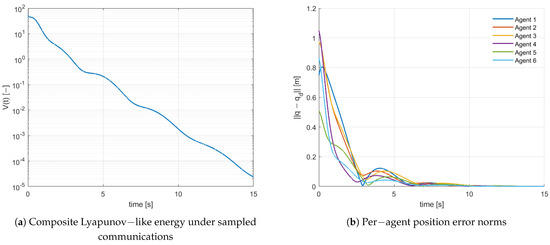 Figure 2. Model stability simulation.
 - 3.
- In the state feedback experiments (Figure 3), the three position and velocity components converge to zero; the position components settle within a few seconds and the velocity components decay even faster. Due to differences in initial conditions and information propagation over the complete topology, the transient responses of different agents show slight variations, but all exhibit consensus and no sustained oscillations.
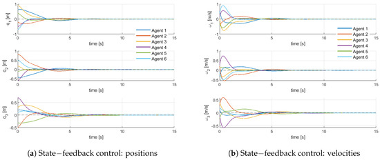 Figure 3. State feedback controller simulation experiment.
 - 4.
- In the velocity observer experiment (Figure 4), the estimated position, , closely tracks the true trajectory, and the estimated velocity, , converges within a few seconds and essentially overlaps the true velocity. Although small ripples may appear at the very beginning due to the sampling-driven estimate used in the observer, the errors decay rapidly, demonstrating that, under discrete communications, the implementable structure achieves accurate velocity reconstruction.
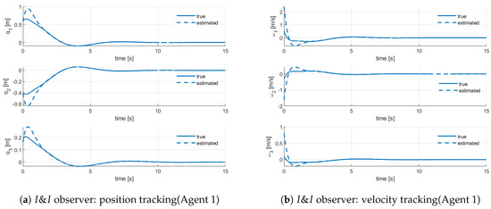 Figure 4. velocity observer simulation experiment.
 - 5.
- As shown in Figure 5, the proposed method achieves superior performance in terms of faster position error convergence, higher velocity estimation accuracy, and smoother control effort compared to the output–feedback strategy presented in [34]. These advantages are critical in multi-agent systems with discrete communication and limited sensor information. The proposed observer-based control framework effectively reduces tracking error and improves robustness against sampling disturbances, demonstrating its practical applicability.
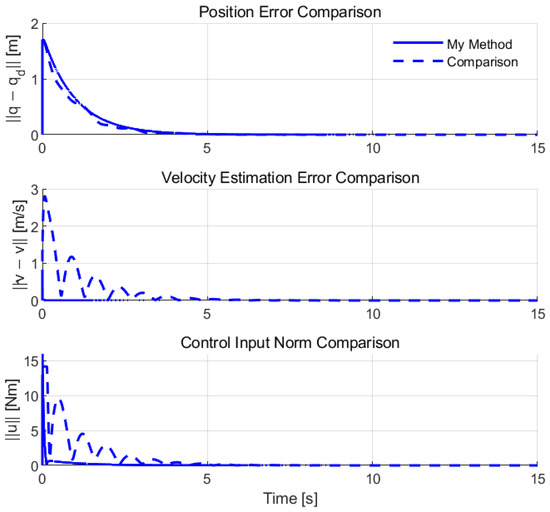 Figure 5. Performance comparison of the two methods.
 - 6.
- As shown in Table 3, to quantitatively assess the performance of the proposed velocity observer, we compute the root mean square error (RMSE) between the estimated and true velocity states of the agents. The RMSE is calculated as
Table 3. Synchronization performance metrics.We also analyzed the convergence time. The simulation results show that the proposed method achieves convergence within 7 s for all agents. Additionally, we computed the communication error rate (CER), defined as the fraction of missed or delayed updates in the velocity state estimates. The error rate is calculated as follows:The CER is showing that the error rate remained below 6% even under the most challenging sampling intervals.
- 7.
- As shown in Table 4, to validate the proposed observer, we compare it with two baseline methods: the Extended Kalman Filter (EKF) and the high-gain observer (HGO). The EKF uses the linearized outer-loop dynamics with the measurement modeland applies Euler discretization. The HGO is implemented aswhere is chosen to balance fast error decay and noise amplification. All methods share the same initial conditions, noise realizations, and neighbor signals.
Table 4. Performance statistics across Monte Carlo (Agent 1).We conduct independent Monte Carlo trials, varying initial perturbations and noise. Performance is evaluated using three metrics: RMSE, Maximum error (Max), and Steady-State Error (SSE), defined asThe results show that the observer consistently outperforms EKF and HGO, achieving lower RMSE and smaller SSE variability under identical conditions.
In summary, for , s, and the specified gains, the system remains stable under the sampled communications, the state feedback achieves multi-agent consensus, and the observer provides effective velocity estimation, offering empirical support for the proposed method.
7. Discussion
This section compares the proposed approach with several representative state-of-the-art methods in terms of performance, robustness, computational complexity, and applicability.
- 1.
- Performance and convergence speed
Traditional robust control methods, such as delay-dependent Lyapunov criteria [21], typically rely on conservative assumptions and can only guarantee asymptotic stability. In contrast, by incorporating sampling-interval-dependent terms into a composite Lyapunov function, our method establishes strict exponential convergence conditions. The simulation results confirm that the proposed framework achieves faster error convergence while tolerating larger communication intervals, outperforming sampled-data control strategies such as [35].
- 2.
- Robustness and adaptability
Many existing works assume full state availability or employ high-gain observers, which are sensitive to noise and non-uniform sampling. Our -based adaptive observer avoids these assumptions and guarantees exponential convergence of estimation errors under discrete and non-uniform communication.
- 3.
- Computational complexity
Event-triggered and game-theoretic approaches [12] often involve complex triggering conditions or optimization problems, making them difficult to implement in resource-constrained distributed robotic systems. In contrast, our design uses low-order linear structures for both the controller and observer. Parameter tuning reduces to solving LMIs, which is computationally efficient and implementation-friendly.
- 4.
- Engineering applicability
Most existing methods are developed under continuous or idealized communication assumptions. Our framework directly addresses discrete and non-uniform communication environments, making it particularly suitable for applications such as cooperative agricultural robotics under bandwidth-limited and delay-uncertain networks.
In summary, the proposed method demonstrates clear advantages over representative existing methods in performance, robustness, computational efficiency, and engineering applicability, thereby providing a practical and effective solution for synchronization control of multi-agent systems under discrete communication conditions.
8. Conclusions
This paper presents a linear multi-agent synchronization control framework based on Immersion and Invariance () theory, providing a comprehensive solution to the challenges of synchronization and state unmeasurability under discrete communication constraints. First, the synchronization control problem is reformulated as a convergence analysis of the error dynamics through state-variable transformation. A composite Lyapunov function, incorporating the sampling mechanism, is constructed, and the Schur complement lemma, in conjunction with Jensen’s inequality, is applied to rigorously derive sufficient conditions for exponential convergence, thereby delineating the impact of sampling intervals on synchronization performance [36]. Building upon this stability analysis, a linear-state feedback controller is designed to ensure closed-loop asymptotic stabilization of the error state within bounded communication intervals, facilitating velocity convergence [35]. To solve unmeasurable velocity, a velocity observer based on I&I theory was proposed. This observer achieves exponential convergence of the velocity estimation error through error-dynamics modeling and observer structure design. Finally, simulation experiments evaluate synchronization performance, control efficacy, and estimation accuracy, demonstrating that the method achieves rapid and stable synchronization under non-uniform sampling communication.
It should be emphasized that the synchronization achieved in this study refers to the exponential convergence of relative state errors rather than the physical co-location of robots. This distinction avoids the misconception that all robots must occupy the same coordinates, highlighting instead the cooperative consistency of trajectories under discrete communication.
Compared to existing methods, this study offers significant advantages in discrete communication adaptability, observer compensation design, and velocity convergence analysis, providing a reliable solution for practical applications, such as cooperative agricultural operations. There remain several promising directions for extending this research [37]. First, the proposed framework can be generalized to more complex nonlinear dynamics, enabling the validation of its applicability in strongly coupled nonlinear environments. Second, energy-constrained implementations will be investigated, ensuring that the controller and observer maintain performance under limited energy budgets, which is especially important for distributed mobile robot systems. Finally, the proposed method will be validated on real robotic platforms, further assessing its effectiveness and robustness in practical engineering scenarios.
Supplementary Materials
The following supporting information can be downloaded at: https://www.mdpi.com/article/10.3390/app15179646/s1.
Author Contributions
Conceptualization, M.L. and H.Q.; methodology, M.L.; software, M.L.; validation, M.L., H.Q. and X.Z.; formal analysis, M.L.; investigation, M.L.; resources, M.L.; data curation, M.L.; writing—original draft preparation, M.L.; writing—review and editing, H.Q. and X.Z.; visualization, M.L. All authors have read and agreed to the published version of the manuscript.
Funding
This research received no external funding.
Data Availability Statement
The original contributions presented in this study are included in the article/Supplementary Material
. Further inquiries can be directed to the corresponding authors.
Conflicts of Interest
The authors declare no conflicts of interest.
Abbreviations
The following abbreviations are used in this manuscript:
| Immersion and Invariance | |
| RMSE | root mean square error |
| CER | communication error rate |
| EKF | Extended Kalman Filter |
| HGO | high-gain observer |
| Max | Maximum error |
| SSE | Steady-State Error |
References
- Mana, A.; Allouhi, A.; Hamrani, A.; Rehman, S.; El Jamaoui, I.; Jayachandran, K. Sustainable AI-based production agriculture: Exploring AI applications and implications in agricultural practices. Smart Agric. Technol. 2024, 7, 100416. [Google Scholar] [CrossRef]
- Lyapunov, A.M. The general problem of the stability of motion. Int. J. Control 1992, 55, 531–534. [Google Scholar] [CrossRef]
- Poincaré, H. Les Méthodes Nouvelles de la Mécanique Céleste; Gauthier-Villars et Fils, Imprimeurs-Libraires: Paris, France, 1893; Volume 2. [Google Scholar]
- Kalman, R.E. A new approach to linear filtering and prediction problems. Trans. ASME–J. Basic Eng. 1960, 82, 35–45. [Google Scholar] [CrossRef]
- Haken, H. Synergetics: An overview. Rep. Prog. Phys. 1989, 52, 515. [Google Scholar] [CrossRef]
- Winfree, A.T. The Geometry of Biological Time; Springer: Berlin/Heidelberg, Germany, 1980; Volume 2. [Google Scholar]
- Kuramoto, Y. Self-entrainment of a population of coupled non-linear oscillators. In Proceedings of the International Symposium on Mathematical Problems in Theoretical Physics, Kyoto, Japan, 23–29 January 1975; pp. 420–422. [Google Scholar]
- Moorthy, S.; Kuppusami Sakthivel, S.S.; Joo, Y.H.; Jeong, J.H. Distributed Observer-Based Adaptive Trajectory Tracking and Formation Control for the Swarm of Nonholonomic Mobile Robots with Unknown Wheel Slippage. Mathematics 2025, 13, 1628. [Google Scholar] [CrossRef]
- Bertsekas, D.; Tsitsiklis, J. Parallel and Distributed Computation: Numerical Methods; Athena Scientific: Nashua, NH, USA, 2015. [Google Scholar]
- Luenberger, D. Observers for multivariable systems. IEEE Trans. Autom. Control 1966, 11, 190–197. [Google Scholar] [CrossRef]
- Astolfi, A.; Ortega, R. Immersion and invariance: A new tool for stabilization and adaptive control of nonlinear systems. IEEE Trans. Autom. Control 2003, 48, 590–606. [Google Scholar] [CrossRef]
- Marden, J.R.; Shamma, J.S. Game theory and control. Annu. Rev. Control Robot. Auton. Syst. 2018, 1, 105–134. [Google Scholar] [CrossRef]
- Zhou, X.; Xu, Y.; Du, S.; Zhao, Q. Immersion and Invariance Adaptive Control for Unmanned Helicopter Under Maneuvering Flight. Drones 2025, 9, 565. [Google Scholar] [CrossRef]
- Huang, S.; Xiong, L.; Zhou, Y.; Gao, F.; Jia, Q.; Li, X.; Li, X.; Wang, Z.; Khan, M.W. Distributed predefined-time control for power system with time delay and input saturation. IEEE Trans. Power Syst. 2024, 40, 151–165. [Google Scholar] [CrossRef]
- Zhang, J.X.; Xu, K.D.; Wang, Q.G. Prescribed performance tracking control of time-delay nonlinear systems with output constraints. IEEE/CAA J. Autom. Sin. 2024, 11, 1557–1565. [Google Scholar] [CrossRef]
- Wang, S.; Ding, J.; Ji, Y. Adaptive immersion and invariance tracking and synchronization control for multi-motor driving systems with parameter uncertainties. IEEE Trans. Transp. Electrif. 2024, 10, 9987–9995. [Google Scholar] [CrossRef]
- Pan, Y.; Yang, Y.; Yi, C. Group Consensus Using Event-Triggered Control for Second-Order Multi-Agent Systems under Asynchronous DoS Attack. Appl. Sci. 2024, 14, 7304. [Google Scholar] [CrossRef]
- Yu, X.; Yang, Y.; Qing, N. Finite-Time Pinning Event-Triggered Control for Bipartite Consensus of Hybrid-Order Heterogeneous Multi-Agent Systems with Antagonistic Links. Appl. Sci. 2024, 14, 9468. [Google Scholar] [CrossRef]
- Li, C.; Li, P.; Zheng, C.B.; Guo, H.; Dong, Z. Event-Triggered Active Fault-Tolerant Predictive Control for Networked Multi-Agent Systems with Actuator Faults and Random Communication Constraints. Appl. Sci. 2025, 15, 6317. [Google Scholar] [CrossRef]
- Khalil, H.K. Nonlinear Systems, 3rd ed.; Prentice Hall: Hoboken, NJ, USA, 2002. [Google Scholar]
- Wu, M.; He, Y.; She, J.H.; Liu, G.P. Delay-dependent criteria for robust stability of time-varying delay systems. Automatica 2004, 40, 1435–1439. [Google Scholar] [CrossRef]
- Chen, C.; Gao, X.; Xiang, Z. Event-Triggered Connectivity-Preserving Consensus of Multiagent Systems Under Directed Graphs. IEEE Trans. Syst. Man Cybern. Syst. 2024, 54, 7230–7239. [Google Scholar] [CrossRef]
- Li, Y.; Cai, Y.; Wang, Y.; Li, W.; Wang, G. Simultaneous tracking and stabilization of nonholonomic wheeled mobile robots under constrained velocity and torque. Mathematics 2024, 12, 1985. [Google Scholar] [CrossRef]
- Petrov, P.; Kralov, I. Exponential Trajectory Tracking Control of Nonholonomic Wheeled Mobile Robots. Mathematics 2024, 13, 1. [Google Scholar] [CrossRef]
- Xiang, Z.; Li, P.; Chadli, M.; Zou, W. Fuzzy optimal control for a class of discrete-time switched nonlinear systems. IEEE Trans. Fuzzy Syst. 2024, 32, 2297–2306. [Google Scholar] [CrossRef]
- Yang, J.; Chen, G.; Zhang, M.; Li, G.; Liu, J. Velocity Observer Design for Tether Deployment in Hamiltonian Framework. Aerospace 2024, 11, 1047. [Google Scholar] [CrossRef]
- Que, H.; Wu, Z.G.; Su, H. Globally exponential synchronization for dynamical networks with discrete-time communications. J. Frankl. Inst. 2017, 354, 7871–7884. [Google Scholar] [CrossRef]
- Lu, J.; Ho, D.W.; Cao, J. A unified synchronization criterion for impulsive dynamical networks. Automatica 2010, 46, 1215–1221. [Google Scholar] [CrossRef]
- Wang, Y.W.; Xiao, J.W.; Wen, C.; Guan, Z.H. Synchronization of continuous dynamical networks with discrete-time communications. IEEE Trans. Neural Netw. 2011, 22, 1979–1986. [Google Scholar] [CrossRef]
- Zou, W.; Guo, J.; Ahn, C.K.; Xiang, Z. Sampled-data consensus protocols for a class of second-order switched nonlinear multiagent systems. IEEE Trans. Cybern. 2022, 53, 3726–3737. [Google Scholar] [CrossRef]
- Romero, J.G.; Nuno, E. Global Stabilization of Nonholonomic Mobile Robots via a Smooth Output Feedback Time-Varying Controller. In Proceedings of the 2019 IEEE 15th International Conference on Control and Automation (ICCA), Edinburgh, UK, 16–19 July 2019; pp. 393–398. [Google Scholar] [CrossRef]
- Hao, L.; Zhang, Y. Event-Triggered Disturbance Estimation and Output Feedback Control Design for Inner-Formation Systems. Appl. Sci. 2024, 14, 3656. [Google Scholar] [CrossRef]
- Rehák, B.; Lynnyk, A.; Lynnyk, V. Synchronization of multi-Agent systems composed of second-Order underactuated agents. Mathematics 2024, 12, 3424. [Google Scholar] [CrossRef]
- Liu, J.; Wang, M.; Wang, H.; Li, W.; Liu, F. Distributed Output-feedback Tracking Control for A Class of Nonlinear Multi-agent Systems with Polynomial Growth. IEEE Access 2024, 12, 160245–160253. [Google Scholar] [CrossRef]
- Huo, B.; Ma, J.; Du, M.; Yin, L. Average consensus tracking of weight-balanced multi-agent systems via sampled data. Mathematics 2024, 12, 674. [Google Scholar] [CrossRef]
- Nguyen, K.H.; Kim, S.H. Improved Sampled-Data Consensus Control for Multi-Agent Systems via Delay-Incorporating Looped-Functional. Mathematics 2025, 13, 299. [Google Scholar] [CrossRef]
- Yang, J.; Li, R.; Gan, Q.; Huang, X. Zero-sum-game-based fixed-time event-triggered optimal consensus control of multi-agent systems under FDI attacks. Mathematics 2025, 13, 543. [Google Scholar] [CrossRef]


Disclaimer/Publisher’s Note: The statements, opinions and data contained in all publications are solely those of the individual author(s) and contributor(s) and not of MDPI and/or the editor(s). MDPI and/or the editor(s) disclaim responsibility for any injury to people or property resulting from any ideas, methods, instructions or products referred to in the content. |
© 2025 by the authors. Licensee MDPI, Basel, Switzerland. This article is an open access article distributed under the terms and conditions of the Creative Commons Attribution (CC BY) license (https://creativecommons.org/licenses/by/4.0/).