Abstract
The article deals with the evaluation of dimensional deformations of a building element manufactured additively from a cement mixture. The study follows up on previous research within the 3DStar project and expands the methodology for monitoring deformations over time. The aim is to contribute to the development of more accurate simulation models for predicting the behaviour of printed structures, especially in the early stages after printing. For the analysis, an experimental ‘L’-shaped element was designed and printed, whose deformations were monitored using repeated 3D scanning and dimensional changes were evaluated for up to 93 days. The results show that the most significant deformations occur in the first hours after printing due to gravitational loading and mixture curing, while later changes are mainly due to shrinkage. The element’s geometry and the walls’ thickness also play a role. The analysis confirms the effectiveness of the ‘Caliper’ measurement method and outlines the potential for future use of photogrammetry as a method for online deformation monitoring. The data obtained will be used to optimise printing parameters and calibrate material parameters in the developed simulation software for non-linear numerical simulations in additive manufacturing using cement mixtures.
1. Introduction
In recent years, additive technologies have seen rapid development and widespread use in many areas. In mechanical engineering, 3D printing is now an everyday reality. Although it is becoming increasingly common in the civil engineering sector, 3D printing is not yet a common practice in this field. The first studies and experiments using modern additive technologies for 3D printing of large objects from cement mixtures date back to the turn of the millennium [1,2]. A wide range of structures have already been built around the world, from buildings [3,4,5], bridges [6,7], etc., to various design and urban elements [8].
The application of 3D printing in civil engineering, primarily based on cement-based mixtures, is proving to be a promising alternative to traditional building methods. This innovative approach allows for the construction of complex geometries and customised structures, which is usually difficult with conventional construction techniques. The unique properties of 3D printing with cement mixtures, where printing is generally carried out by extruding individual layers at a time, offer significant advantages in terms of design flexibility, reduced labour costs, and minimised material waste [9,10,11].
The sustainability aspect of 3D-printed concrete also deserves attention. The civil engineering industry is under increasing pressure to reduce its carbon footprint, and 3D printing technology offers a way to achieve this goal. Using alternative materials, such as recycled aggregates or industrial by-products, can significantly reduce the environmental impact of concrete manufacturing [11,12]. In addition, the overall sustainability of 3D printing in construction is enhanced by reducing construction waste and the possibility of manufacturing building elements directly on-site [13,14].
One of the key factors influencing the success of 3D-printed concrete is the composition of the cement mixtures used. These mixtures must have specific rheological properties to ensure proper fluidity and workability during printing. Research suggests that suitable concrete mixtures for 3D printing typically exhibit lower viscosity and higher workability than traditional concrete, allowing for easy extrusion through a nozzle [10,15]. In addition, these mixtures require fast setting times to support the weight of subsequent layers while maintaining structural integrity [16,17]. Optimising these properties is essential to achieving high-quality printed structures that can withstand various environmental influences and mechanical stresses.
The mechanical properties of 3D-printed cement mixtures are also a focus of ongoing research. Studies have shown that mechanical properties, including compressive, flexural, and tensile strength, can vary significantly depending on the mixture design and printing parameters [11,17]. For example, incorporating additives such as fibres, reinforcements, or supplementary cementitious materials can improve the properties of 3D-printed concrete, leading to improved durability and crack resistance [18,19,20,21]. Understanding the interaction between material properties and the printing process is essential for developing robust and reliable 3D-printed structures.
Advanced inspection methods are an effective way to ensure the quality of 3D-printed objects. Traditional manual inspection methods are often time-consuming and prone to human error, highlighting the need for automated and accurate inspection techniques [22,23]. Recent studies have demonstrated the effectiveness of laser scanning and photogrammetry in assessing the dimensional accuracy of printed structures made from cement mixtures, achieving measurement accuracy in the range of millimetres [24,25]. These technologies facilitate a detailed comparison of the intended design and the actual printed object, allowing the identification of discrepancies that could compromise the properties of the structure [26,27]. Another example is studies evaluating the geometric accuracy of printed sample parts after printing [28,29]. More commonly, the evaluation of print quality online during construction is carried out by integrating various sensors to monitor important parameters of the entire 3D printing process [30,31,32]. It is possible to check and, if necessary, influence the quality of printed objects through feedback. A comprehensive review [33] describes the possibilities for inspection at all stages of the 3D printing process using cement mixtures, including an overview of the specific technologies and equipment used for quality control.
This study builds on previous research [34] conducted as part of the 3DStar project. While our prior work introduced a robust methodology for monitoring overall deformations and checking the quality of 3D printing over time in terms of the hardening and curing of cement mixtures, the current study significantly expands on it by introducing a more detailed analysis of the structural behaviour of the element. Specifically, we focus on evaluating the deformations of an L-shaped element designed with variable wall thicknesses and a more complex internal arrangement. Detailed thickness mapping in a point matrix allows a deeper understanding of local shape changes. This comprehensive approach will enable us to determine the deformation of the building element over time as accurately as possible, especially in the early stages after printing. This is key to fine-tuning the cement mixture parameters and improving the parallel printing simulation model being developed by colleagues from the project team. This work also verifies the real-time printing time against the calculated G-code predictions. This is key in refining the material parameters and ensuring the correct input values for the simulation algorithm being developed. This will allow us to assess the feasibility of 3D printing, especially for more complex building structures, even before implementation.
2. Materials and Methods
2.1. Print Preparation
An ‘L’-shaped wall element with internal structures and external nominal dimensions of 1200 × 500 × 700 mm was designed for shrinkage and deformation analysis. To assess the effect of the thickness of the printed wall on shrinkage, one wall was chosen as single (one print path) and the other (shorter) wall as double (two print paths side-by-side). Printing was planned for a circular nozzle with a diameter of 20 mm and a layer thickness of 10 mm. Slicer4ATENA v. 1.1 proprietary software was used to prepare the print and generate the print head paths. The result was an NC programme generated for the actual 3D printing after being uploaded to the machine control system. The calculated time was added as a comment in each line of the generated NC programme for easy and quick checking of the actual and computed time; see Figure 1.
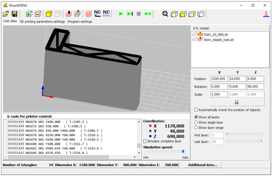
Figure 1.
Preparation of a printed element in the Slicer4ATENA software.
2.2. Printing
Printing was performed on a three-axis device with a Cartesian coordinate system and its application head. The working area of this machine is 3500 × 1100 × 1300 mm (X, Y, Z). The maximum feed rate is 3 m/s on the X- and Y-axes and 2 m/s on the Z-axis. Positioning repeatability is better than 0.3 mm on all axes. For more detailed parameters, see [35].
A specially developed cement-based mixture was used as the building material. The mix included individually selected components typical for fine-grained micro-concrete (silica sand 0–1.25 mm, microfillers, CEM II 52.5, microsilica). The ratio of the components is confidential, but ensures the mixture meets requirements for mechanical and physical properties, workability, pumpability, and stiffness after extrusion from the print head. The mixture was supplemented with dispersed PP reinforcing fibres concerning thixotropy and reduced shrinkage. For continuous printing, it was necessary to accelerate the hardening process of this mixture with a liquid accelerator injected into the print head. Although this acceleration caused some degradation of the mechanical properties, it allowed for continuous printing of the wall element without the risk of collapse. The reference material without an accelerator has a flexural tensile strength of 10.5 MPa and a compressive strength of 59.0 MPa (after 28 days). The mix with the accelerator has a flexural tensile strength of 6.3 MPa and a compressive strength of 44.5 MPa (after 28 days) [34].
Due to the relatively high printing speed of 100 mm/s and the inertia of the extruder, the extrusion was not switched off when moving to the next layer, resulting in a noticeable overflow of material in the starting corner of the object. Furthermore, due to slight over-extrusion, the quality of individual layers was affected, especially at the connection points of individual internal ribs, etc. The printed ‘L’-shaped wall element is shown in Figure 2. Its total printing time was approximately 1 h.
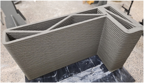
Figure 2.
Printed ‘L’-shaped wall element.
Printing of the given object was carried out in laboratory conditions, i.e., at a temperature of approximately 21 °C and relative humidity of approximately 40%. After printing, the object was left in similar conditions in the same laboratory for the entire duration of the testing, i.e., no additional curing or tempering was performed. Finally, no visible cracking due to shrinkage occurred during the whole monitoring period.
2.3. Digitisation and Inspection
A MetraSCAN 350 optical 3D scanner (Creaform, Lévis, QC, Canada) was used to digitise the printed wall element. It is a dual-camera non-contact system that uses an optical tracking unit—C-track—for positioning in 3D space. This system allows scanning in a space of up to 16.6 m3 without using reference marks for the measured object. According to the manufacturer, the system’s accuracy throughout the working space is up to 0.12 mm. This is also confirmed by the calibration of the entire system, which was performed for every new day of scanning according to the manufacturer’s methodology and standards. The maximal calibration error was 0.022 mm for the C-track, and for the scanning head, it was 0.072 mm (see Figure 3).
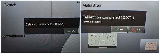
Figure 3.
Results of user calibration of C-track and MetraScan.
This analysis primarily focuses on monitoring the shape and dimensional deformations of the printed element over time. The segment was scanned immediately after completion of the printing process (further referred to as time ‘0’ or model ‘0’) and then scanned again at intervals of 20, 40, 60, 90, 120, and 180 min, then 22 h, and finally 28 and 93 days (see Figure 4). Digitisation was repeated twice at 22 h, 28, and 93 days. Due to the small number of repetitions, it was not relevant to apply statistical evaluation of the results; the repetitions served mainly for self-checking of the output data. Between 0 and 3 h, it was not technically possible to repeat the scan, as the repeated scans would have been performed at a different time (one scanning cycle took approximately 10 min). In addition to the nominal CAD model, 14 scans of the printed wall element were available.
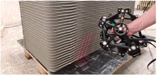
Figure 4.
Scanning the wall element with the MetraScan system.
A resolution of 1 mm was selected for scanning the wall element. During previous testing, this value proved to be an ideal compromise between scanned details and data requirements and the speed of the entire scanning process. The result of the scan is a large number of points describing the object’s surface (a so-called point cloud). After digitisation, an optimised polygonal mesh (a model in STL format) is calculated. This mesh can then be further processed using inspection software GOM Inspect Professional, v. 2018 (Carl Zeiss GOM, Braunschweig, Germany). In this software were performed all dimensional and shape checks (inspections) of the scanned data. All scans and the nominal CAD model were imported into this programme into a single project as a so-called STAGE. In addition to comparing the nominal CAD model, this also allows the comparison of individual models with each other, with the option of selecting which STAGE is the reference. In the case of calculating colour maps of deviations and dimensional changes, model ‘0’ was chosen as the reference, i.e., the sample was scanned immediately after printing. This eliminates errors from the 3D printing process itself.
The first step was to align all scans in the coordinate system. Then, the inspection itself was performed—in our case, colour maps of deviations from the CAD model and from the reference model (the model scanned immediately after printing—time ‘0’) were calculated. Finally, the main length dimensions were measured in all three directions of the coordinate system.
3. Results and Discussion
In this work, several methods proposed in a previous study [34] were used to evaluate the shape changes of the ‘L’-shaped wall element. For quick analysis, colour maps of deviations from the reference model ‘0’ were calculated at individual time steps. Colour maps allow quick visual inspection and a comprehensive view of deformations and dimensional changes in the colour spectrum—they express normal deviations from the reference model ‘0’ (warm shades—positive deviation, cold shades—negative deviation). Aligning individual models within the coordinate system is important for interpreting colour deviation maps. In this case, the alignment was uniform within a single scanning day (i.e., at 20 and 40 min, 1, 1.5, 2, 3, and 22 h) and was determined by the C-Track coordinate system. Models from other scanning days (when, for technical reasons, it was not possible to maintain the same C-track position and thus a uniform global coordinate system) were first aligned using BestFit function to the model from the previous scan and then aligned using Local BestFit function on the Z-axis to the position of the base plate plane. Due to the typical surface structure of the wall element given by 3D printing, deformations cause displacement over time and, thus, partial overlap of the individual printed layers. Therefore, colour maps are not very informative when comparing individual scans with each other, and it is difficult to analyse dimensional changes accurately over time. An example of the resulting colour map of the tested object is shown in Figure 5.
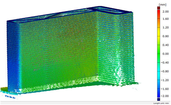
Figure 5.
Colour map showing deviations from the reference sample ‘0’ after 93 days.
Therefore, measurements of the length dimensions on three axes (on the X-axis, the length of the shorter wall; on the Y-axis, the length of the longer wall; on the Z-axis, the height of the printed element) were performed in all scans. Based on experience from previous research, detailed measurements of the distance between opposite walls were taken at several horizontal levels using the ‘Caliper’ function (see Figure 6). The method is based on the principle of a sliding gauge, where two parallel discs touch the outside of the selected area. The software creates two touchpoints where the discs first touch the element. The result is the calculated distance between the two touchpoints in a given direction. For the measurement, the disc diameter was set to 30 mm (to cover approximately three layers). In addition to the absolute dimensions, the results for each state were compared with the reference model (time ‘0’) and the deviations were calculated.
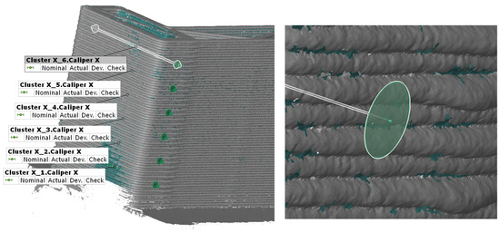
Figure 6.
Local distance measurement using the ‘Caliper’ function—wall length along the X-axis.
On the X- and Y-axes (wall length), measurements were taken at six height levels every 100 mm (marked Xi, Yi: the index ‘i’ denotes the height level), always on the axis of the given wall. In the Z direction (height), so-called ‘labels’ were created on the top surface (last printed layer), which directly express the deviation from the reference model (time ‘0’); see Figure 7. The labels were divided into two groups: the first group (labelled ‘single’) consisted of labels created on the wall printed with a single path, and ‘double’ labels were made on a wall printed with two parallel paths.
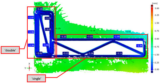
Figure 7.
Colour map of deviations and labels with height deviations from the ‘0’ state (93 days).
In addition to length measurements, detailed measurements of the thickness of the longer walls were performed. The measurements were taken at the same height levels as the previous length measurements (100, 200, 300, 400, 500, and 600 mm) in five vertical sections (i.e., measured at 30 points in total); see Figure 8.
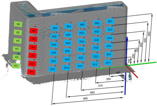
Figure 8.
Marking of points for dimensions Xi (red labels), Yi (green labels), and wall thickness Xij (blue labels).
The positions of these sections were chosen concerning the position of the internal ribs so that the measurements were taken both at the point where the rib connects to the outer wall and in the middle of the stretch between these connections. The distances of the cuts from the zero point on the Y-axis were chosen as 185, 350, 515, 680, and 845 mm—marked Xij: the index ’i’ denotes the height level, and the index ‘j’ represents the position number of the vertical cut on the Y-axis. At the cut at a distance of 350 mm, an internal reinforcement rib is connected to the rear wall, and at the cut at a distance of 680 mm, this rib is connected to the front wall. The marking method is shown in more detail in Figure 8.
It should be noted that the results are very sensitive to the quality of the scan. Due to the nature of the functions used (mainly point or envelope measurements), unexpected errors may occur in some instances due to defects in the scan. It is one of the reasons why the scanning and evaluation (where possible) were repeated, and the results were averaged from these repeated measurements. Repeated measurements carried out at 22 h, 28 days, and 93 days showed that the variability did not exceed ±0.05 mm, corresponding to the specified accuracy of the scanner.
The following graphs show changes in dimensions as a function of time on the X-axis (see Figure 9) and on the Y-axis (see Figure 10). Dimensions on the X-axis—nominal length 500 mm—are measured on the ‘L’-shaped part of the object with a double wall; see red labels in Figure 8. Dimensions on the Y-axis—nominal length 1200 mm—are measured on the longest wall of the ‘L’-shaped object; see green labels in Figure 8. In both cases, two types of dimensional changes are apparent—especially in the early stages after printing, deformation and bulging of the walls occur due to the load from the upper layers of the material, while later, shrinkage occurs almost exclusively, which is caused by drying and chemical changes in the material.
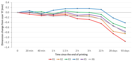
Figure 9.
Dimensional changes of the wall element over time on the X-axis (Caliper).
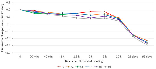
Figure 10.
Dimensional changes of a wall element over time on the Y-axis (Caliper).
In the X-axis direction (double wall), deformation and bulging are the most noticeable around the centre of the wall element height (dimensions X3 and X4). This deflection does not occur in the lower layers, which is probably due to the fixation of the dimensions of the first layers thanks to adhesion to the base, which is larger due to the double wall. However, a more significant role is played here by a systematic error caused by the measurement method used, where the first scan of the object was performed after it had been entirely printed—the so-called ‘time 0’. However, the first layer is about one-hour old, i.e., time ‘0’ is only valid for the last layer. Unfortunately, online scanning of the object during printing is impossible in this way. This error is most pronounced in the first hours after printing, but loses significance as time passes.
Measurements of time-dependent deformations in the Y-axis direction are performed perpendicularly to the short side walls. As demonstrated in a previous analysis, these are not so sensitive to deformation and bulging [34]. Here, only slight bulging of the lower layers is apparent between the second and third hours, which is mainly influenced by the load from the upper layers. Both graphs also show that, 22 h after the end of printing, all curves are more or less equidistant, which means that the printed object is already so rigid that it does not deform due to gravity but almost exclusively due to shrinkage.
The graph in Figure 11 shows the deformation over time for the vertical direction—the Z-axis (nominal height 700 mm). The change in wall thickness has almost no effect on the deformation of the printed object in this direction. The height difference at the various points at a given time is around 0.1 mm, which is an insignificant value. Although the statement from the previous analysis [34] that higher-volume parts of the element shrink more slowly than thin ones is true, it is not significant here.
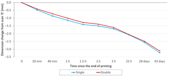
Figure 11.
Dimensional changes of the wall element over time on the Z-axis (Label).
The following graphs show the summary results for all three monitored directions, with the values on the X- and Y-axes averaged across all height levels. Similarly, the values on the Z-axis are also averaged for single and double walls. The resulting deviations are expressed as absolute error (see Figure 12) and relative (percentage) error (see Figure 13 and Figure 14). The graph in Figure 14 represents the time linearly for a more straightforward overview of the object’s deformation.
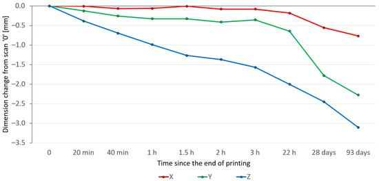
Figure 12.
Average dimensional changes of the wall element over time (absolute, time axis according to measurements).
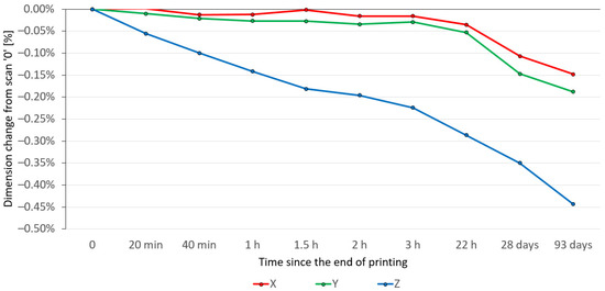
Figure 13.
Average dimensional changes of the wall element over time (relative in %, time axis according to measurements).
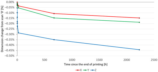
Figure 14.
Average dimensional changes of the wall element over time (relative in %, linear time axis).
Dimensional changes represented relatively in the graph in Figure 13 indicate that the deformations and subsequent shrinkage in the X- and Y-axes are essentially similar. A slight difference may be due to the different wall thicknesses of the printed object. In the X-axis direction, both opposite walls are printed with double thickness, while in the Y-axis direction, one wall is double and the other is single. As expected, the most significant change in dimensions can be seen in the vertical direction—the Z-axis—caused by the settling of the object due to gravity and later by the shrinkage of the object during the hardening of the cement mixture.
The graph in Figure 14 shows the same values as the previous one but with a linear time scale. It clearly shows how the printed object changed over time in different directions. As expected, the most significant change in dimensions occurred in the first hours after printing, especially on the Z-axis. After about one day, the wall element begins to shrink relatively slowly.
The following graphs show the results of measurements of the thickness of the thin, longer wall of the ‘L’ wall element (nominal thickness 200 mm and length 1000 mm), or rather the deviations of these values from the reference model (time ‘0’). Measurements in this direction are the most complicated and difficult to predict. As mentioned above, wall deformations were measured in the direction of the length and height of the object at a total of 30 points; see blue labels Xij in Figure 8. The assumption is that spatial deformations of the object are most significantly reflected in the thickness direction of this part of the sample. Many variables, such as the shape of the printed object, the position of the internal ribs, the printing quality, the speed of solidification of the mixture, etc., influence these.
As this is a relatively large amount of data, the values are presented in a simplified form in the following graphs. This simplification consists of averaging the values of length changes in the selected direction so that their dependence on time can be expressed as a curve.
The graph in Figure 15 shows the time dependence of wall deformation of the averaged values of vertical sections Xi1 to Xi5. It expresses the average deviations over time along the length of the object.
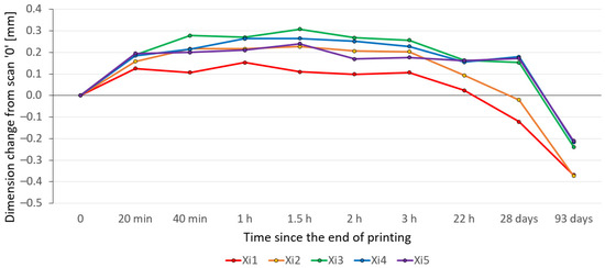
Figure 15.
Dimensional changes of wall thickness over time on the X-axis in individual vertical sections (‘Xij’).
At first view, it can be seen that the wall thickness increased relatively quickly along its entire length, regardless of the internal ribs or the connection to the shorter part of the ‘L’ element printed with double wall thickness. This is mainly due to spatial deformations of the element due to the bulging of the uncured mixture at that moment. The relatively smallest change in wall thickness is at its free end—the red curve Xi1. This is probably due to the relatively short distance from the perpendicular end of the wall element, which prevents this bulging from occurring more effectively than the diagonal inner rib.
The graph in Figure 16 shows the time dependence of wall deformation of the average values of horizontal sections X1j to X6j. It represents the average deviations over time at individual height levels of the object. Again, significant deformation can be seen from the very first minutes. This deformation is more pronounced in the upper layers, causing the object to open up. This is due to the fixation of the dimensions of the first layers, thanks to adhesion to the base plate, and also to the already-mentioned systematic measurement error, where the first layers of the object are about an hour older than the top layers.
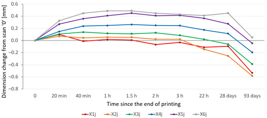
Figure 16.
Dimensional changes of wall thickness over time on the X-axis in individual height levels (‘Xij’).
While the above results show average deviations across given height levels or vertical sections, below is a more detailed view of the distribution of deviations across the entire wall surface from the initial state in the form of a matrix entry at selected times (1.5 h, 22 h, and 93 days), see Table 1. This numerical expression illustrates the complexity of the shape deformation of the wall element in terms of its thickness. The table has the same matrix cell layout as the position of the measuring points in Figure 8, and the sizes of the deformations are colour-coded for greater clarity. As the shade of red deepens, the dimensions of the element increase; as the shade of blue deepens, the wall thickness decreases.

Table 1.
Dimensional changes of the thin wall in the matrix at 1.5 h, 22 h, and 93 days.
The first hours after printing mainly involve spatial deformation of the wall element due to the bulging of the mixture, which is not yet mature. This deformation is most pronounced from the element’s centre upwards in the shape of a wide letter ‘V’. Later, shrinkage due to the curing of the cement mixture is most notable, which is essentially constant given the thickness of the wall. This deformation process disappears in the averaged values.
Additionally, analysis of the deformations of the front and rear walls of this part of the structure from its central plane was performed. This further clarifies the wall deformation process, especially concerning the reinforcing elements’ positions. The connection of the internal reinforcement is shown in Table 2 and Table 3 by the grey table header and the bold deformation values.
Table 2.
Changes of the front wall from the central plane at 1.5 h, 22 h, and 93 days.
Table 3.
Changes of the rear wall from the central plane at 1.5 h, 22 h, and 93 days.
While Table 1 shows that the total thickness of this wall increases symmetrically from the centre upwards, a more detailed analysis shows that the front part opens more from the centre to the right and, conversely, the rear part from the centre to the left. The reinforcement rib therefore fulfils its stabilising function during printing, as expected, even though this was not apparent from previous analyses. This is shown in Table 2 and Table 3 at 1.5 h (when deformation and bulging due to gravity still occur). The position of the rib’s contact with the wall is highlighted. It can be seen that the deformation is close to 0 mm in these areas, while the error increases up to 0.5 mm in areas distant from the rib. The trend is also evident in the later stages of the object’s ageing, where the object is mainly shrinking.
This particular deformation was not visible even on the colour deviation maps (see, for example, Figure 5), because the settling of the object on the Z-axis is more significant and, due to the typical structure of the 3D-printed object, this type of object deformation is more or less hidden. Thus, a detailed analysis like this is important for future comparison with deformations calculated using simulation and, especially in the early stages, can serve as an experimental refinement of the mechanical properties of the cement mixture.
However, the disadvantage of this evaluation method is the high sensitivity of the technique used to position the object in the coordinate system, which is relatively laborious and challenging to control. The point is that it uses measurements of distances from a fixed central plane to the front and rear walls of the object. An error due to inaccurate positioning of the object will then also introduce an error into these partial results, whereas measuring the total wall thickness using the ‘Caliper’ method is not affected by the alignment method.
The final milestone of this analysis was to compare the calculated and actual printing times, as these data are another input into the simulation algorithm being developed for simulating the additive manufacturing of objects from cement or other similar mixtures. Therefore, information about the calculated build time was added to the G-code for TestBed in the form of comments, which made it possible to monitor deviations between the theoretical (calculated) time and the actual printing time in real time.
Figure 17 shows a screenshot of the TestBed control system during printing. It displays information about the actual printing time and the calculated time in the preview of the programme currently being printed (G-code). The figure shows the actual printing time, approximately 1863 s at the given point in the programme, while the calculated time is approximately 1877 s. The difference is because the calculation of times from the NC programme only uses a simplified model of the real machine. Despite this, the difference in times after approximately 30 min of printing is less than 1% when printing an ‘L’-shaped wall element.
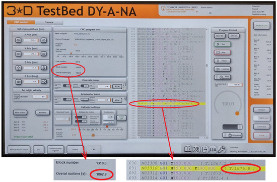
Figure 17.
Screenshot of the TestBed control system during printing—comparison of times.
However, further attention must be paid to comparing times and actual material consumption. Unfortunately, manual interventions to adjust the printing speed or the feeding of material according to the current state of the print, based on previous experiences, are still relatively common. Therefore, it is important to refine the parameters of the entire process based on the results of dimensional and other analyses. The results then serve as a reliable basis for developing a simulation model of 3D printing from cement mixtures.
4. Conclusions
The presented study extends knowledge of 3D printing from cement mixtures and builds on previous research activities within the 3DStar project. The work aimed to verify and expand the methodology for evaluating the dimensional and shape stability of building elements printed using additive technology from cement mixtures over time, i.e., from the moment immediately after printing to a period exceeding three months. Using time-scheduled 3D scanning and subsequent evaluation in the GOM Inspect environment, it was possible to monitor the development of deformations in the basic X, Y, and Z directions. In this study, the progress of shape changes in the first tens of minutes after printing was examined and evaluated in detail. The aim was also to help colleagues develop tools and methods for simulation and quality control for creating and designing digital concrete structures to better estimate material parameters, especially in the so-called wet phase of the cement mixture, based on measured deformations. For this purpose, an experimental ‘L’-shaped object was designed with variable wall thicknesses in different parts and different structural arrangements, which made it possible to analyse the behaviour and shape changes of the element over time in its various parts.
The analysis was performed in the selected coordinate system of the element and was related to the first scan after printing had been completed (time ‘0’). Global visualisation methods (colour deviation maps) were used for quick checks, but the actual evaluation of deformations was based on measuring deviations in length dimensions at pre-planned points. The previous study was further expanded to include a more detailed analysis of the overall dimensions in the given point matrix and the separate deformation of the two walls of the building element.
The results show that in the early period after printing (0–3 h), spatial deformations occur, mainly due to the gravitational load on the immature cement mixture. This takes the form of the walls bulging outwards, the upper layers opening up, and deformations in the thickness of the element, which, however, do not exceed a relative change in dimensions of 0.05% in the horizontal plane at this stage. The vertical settlement of the element is most pronounced at this stage, representing a relative change in dimensions of around 0.3%.
In the medium term (from approximately 3 h to 1 day), a transition between gravitational deformation and volume shrinkage related to cement hydration and water evaporation became evident. The deviations in dimensions began to stabilise, and the curves of dimensional changes in individual directions became equidistant, indicating that the printed element had already achieved sufficient rigidity to resist its load. This phenomenon is well illustrated in Figure 14, where the averaged deformations of the object over time on all three axes are presented relatively in percentages and with the real-time axis.
Long-term changes (22 h to 93 days) are characterised almost exclusively by isotropic shrinkage, which manifests itself in longitudinal and vertical directions, with a relative change of approximately 0.15% in this phase.
The most significant absolute and relative deformations were recorded in the Z-axis (height) direction, where the layers settled. The changes in the X- and Y-axes (wall lengths) are milder and more dependent on the structural geometry. When analysing the thickness of longer walls, significant spatial deformations were observed, which had different courses depending on the height level and position within the length of the element. In simple terms, it can be stated that the upper layers are more prone to bulging. In contrast, the lower layers show higher stability due to adhesion to the base plate and the partial curing of the cement mixture.
Deformation analysis using the ‘Caliper’ function is a robust tool for evaluating dimensional changes over time, even with repeated scanning. In contrast, methods that depend on the precise positioning of the object in the coordinate system, such as measuring deviations from the central plane, were significantly more sensitive to systematic errors and require high precision in scan positioning. However, this method provides even more detailed information about the deformations of the wall element over time.
Unfortunately, the offline scanning method’s disadvantage at pre-planned times also became evident. The problem was that printing the wall element took about 1 h, and then the scanning could begin. During this hour, the cement mixture in the lower layers was already curing, and time ‘0’ only applies to the last printed layer.
A quick analysis comparing the calculated and actual printing times confirmed a high degree of agreement and the suitability of this approach as input for the simulation model, which is being developed in parallel. The results of this work thus not only verify the proposed methodology for monitoring deformations over time but also provide valuable quantitative data for calibrating computational models of this additive technology based on cement mixtures.
Overall, it can be concluded that the proposed experimental methodology allows reliable monitoring of shape changes in objects printed from cement mixtures over time and that spatial deformations in the early stages of printing are a significant factor influencing the final quality of the structure. The results of this study thus contribute to a better understanding of deformation mechanisms, enable more accurate prediction of the final shape of the structure, and represent an important step towards optimising the material and process parameters of 3D printing for practical use in civil engineering.
Further research will focus on implementing online measurement of the following building elements to avoid the disadvantage of evaluating deformations for unequally cured individual layers caused by offline scanning. For this purpose, photogrammetry was tested. As part of a pilot experiment, a printed building element of a similar concept was photographed from many different positions, and a 3D model in STL format was calculated based on these images. The disadvantage of photogrammetry is that it is difficult to obtain the real dimensions of an object from simple photos. This experiment placed calibrated artefacts with coded points in the inspected object’s space. The object’s dimensions were then calculated in the 3D mesh based on the known artefact dimensions. The model of one wall and the colour map of the deviations of the model obtained in this way from the model obtained by 3D scanning with the MetraScan system are shown in Figure 18.
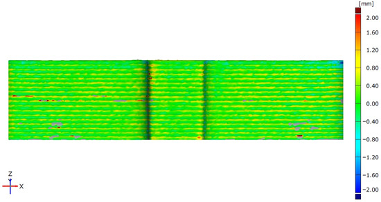
Figure 18.
Colour map of deviations of the model obtained by photogrammetry (20 photos) compared to the 3D scan by the MetraScan system.
It turned out that this method gave results only slightly worse than the scanning used in this study and is therefore usable. Since it is impossible to be in the printer’s workspace and take photos manually while objects are being printed, the plan is to place several tens of cameras directly in the machine’s workspace. These will synchronously capture images of the growing object in real time, which will be used for calculations of digital models of the printed object and dimensional analysis. The advantage of this arrangement is the speed of image acquisition. It is expected that, in theory, it will be possible to take several sets of images of the inspected object per second. Of course, calculating and evaluating the 3D mesh from each set will be significantly slower and performed offline. However, the input images for these calculations are crucial. To a certain extent, this system will also be able to capture dynamic phenomena during the object building. It will allow for even better prediction of the behaviour of the printed element and better tuning of material parameters in the early stages of the developing simulation model, whose task will be to predict the shrinkage and shape behaviour of printed objects using computer numerical simulation.
Author Contributions
Conceptualisation, P.K. and R.M.; methodology, R.M.; validation, P.K. and R.M.; formal analysis, P.K. and R.M.; investigation, P.K. and R.M.; resources, P.K.; data curation, P.K. and R.M.; writing—original draft preparation, P.K. and R.M.; writing—review and editing, P.K.; visualisation, P.K. and R.M.; supervision, P.K. and R.M.; All authors have read and agreed to the published version of the manuscript.
Funding
The research presented in this paper was supported by the Technology Agency of the Czech Republic and the Ministry of Industry and Trade within the TREND Programme ‘digiBeton—Simulation and design of structures from digital concrete’, project ID: FW06010422. The infrastructure used for the research presented in this article was supported by the European Structural and Investment Funds of the Operational Programme Research, Development and Education within the project ‘3D Print in Civil Engineering and Architecture—3D STAR’ reg. number CZ.02.1.01/0.0/0.0/16_025/0007424.
Data Availability Statement
The data presented in this study are available on request from the corresponding author.
Conflicts of Interest
The authors declare no conflicts of interest. The funders had no role in the design of the study; in the collection, analyses, or interpretation of data; in the writing of the manuscript; or in the decision to publish the results.
Abbreviations
The following abbreviations are used in this manuscript:
| 3D | Three-Dimensional |
| CAD | Computer-Aided Design |
| NC | Numerical Control |
| STL | Standard Triangle Language |
References
- Pegna, J. Exploratory Investigation of Solid Freeform Construction. Autom. Constr. 1997, 5, 427–437. [Google Scholar] [CrossRef]
- Buswell, R.A.; Thorpe, A.; Soar, R.C.; Gibb, A.G.F. Design, Data and Process Issues for Mega-Scale Rapid Manufacturing Machines Used for Construction. Autom. Constr. 2008, 17, 923–929. [Google Scholar] [CrossRef]
- Apis Cor. 2021. Available online: https://www.apis-cor.com/ (accessed on 28 January 2025).
- Cobod International A/S Cobod. Available online: https://cobod.com (accessed on 6 February 2025).
- FBR Ltd FBR|Industrial Automation Technology. Available online: https://www.fbr.com.au/ (accessed on 7 February 2025).
- Salet, T.A.M.; Ahmed, Z.Y.; Bos, F.P.; Laagland, H.L.M. Design of a 3D Printed Concrete Bridge by Testing. Virtual Phys. Prototyp. 2018, 13, 222–236. [Google Scholar] [CrossRef]
- Gardner, L.; Kyvelou, P.; Herbert, G.; Buchanan, C. Testing and Initial Verification of the World’s First Metal 3D Printed Bridge. J. Constr. Steel Res. 2020, 172, 106233. [Google Scholar] [CrossRef]
- Anton, A.; Bedarf, P.; Yoo, A.; Dillenburger, B.; Reiter, L.; Wangler, T.; Flatt, R.J. Concrete Choreography: Prefabrication of 3D-Printed Columns; UCL Press: London, UK, 2020; Volume 8, pp. 286–293. [Google Scholar] [CrossRef]
- De Schutter, G.; Lesage, K.; Mechtcherine, V.; Nerella, V.N.; Habert, G.; Agusti-Juan, I. Vision of 3D Printing with Concrete—Technical, Economic and Environmental Potentials. Cem. Concr. Res. 2018, 112, 25–36. [Google Scholar] [CrossRef]
- Panțiru, A.; Luca, B.-I.; Bărbuță, M. Investigations Regarding Concrete Mixes Suitable for 3D Printing. Bulletin of the Polytechnic Institute of Iași. Construction. Archit. Sect. 2022, 68, 151–164. [Google Scholar] [CrossRef]
- Rehman, A.U.; Kim, J.-H. 3D Concrete Printing: A Systematic Review of Rheology, Mix Designs, Mechanical, Microstructural, and Durability Characteristics. Materials 2021, 14, 3800. [Google Scholar] [CrossRef]
- Zhang, Y. 3D Concrete Printing for Sustainable and Efficient Building Practices in Singapore. Acad. J. Archit. Geotech. Eng. 2024, 6, 8–12. [Google Scholar] [CrossRef]
- Valle-Pello, P.; Álvarez-Rabanal, F.P.; Alonso-Martínez, M.; del Coz Díaz, J.J. Numerical Study of the Interfaces of 3D-printed Concrete Using Discrete Element Method. Mater. Werkst. 2019, 50, 629–634. [Google Scholar] [CrossRef]
- Geng, S.; Long, W.; Luo, Q.; Fu, J.; Yang, W.; He, H.; Ren, Q.; Luo, C. Intelligent Prediction of Dynamic Yield Stress in 3D Printing Concrete Based on Machine Learning. Adv. Eng. Technol. Res. 2023, 6, 468. [Google Scholar] [CrossRef]
- Zhang, H.; Wang, J.; Liu, Y.; Zhang, X. Evaluation and Correlation Study on Work Performance of 3D-Printed Concrete. J. Adv. Concr. Technol. 2021, 19, 1181–1196. [Google Scholar] [CrossRef]
- Hui, L.; Lopez Almansa, F. Experimental Test on Drying Shrinkage of 3D-Printed Fiber-Reinforced Concrete at Early Ages. Am. J. Civ. Eng. Archit. 2018, 6, 24–29. [Google Scholar] [CrossRef][Green Version]
- Joh, C.; Lee, J.; Bui, T.Q.; Park, J.; Yang, I.-H. Buildability and Mechanical Properties of 3D Printed Concrete. Materials 2020, 13, 4919. [Google Scholar] [CrossRef] [PubMed]
- Neef, T.; Mechtcherine, V. Simultaneous Integration of Continuous Mineral-Bonded Carbon Reinforcement Into Additive Manufacturing with Concrete. Open Conf. Proc. 2022, 1, 73–81. [Google Scholar] [CrossRef]
- Juhari, H.F.; Ali, N.; Abdullah, S.R.; Salleh, N.; Abdul Hamid, N.A. Fresh Properties and Compressive Strength of 3D Printing Concrete Containing GGBS as Partial Cement Replacement. J. Struct. Monit. Built Environ. 2022, 2, 33–41. [Google Scholar] [CrossRef]
- Spurina, E.; Sinka, M.; Ziemelis, K.; Bajare, D. The Effects of 3D Printing on Frost Resistance of Concrete. J. Phys. Conf. Ser. 2023, 2423, 012037. [Google Scholar] [CrossRef]
- Li, Z.; Hojati, M.; Wu, Z.; Piasente, J.; Ashrafi, N.; Duarte, J.P.; Nazarian, S.; Bilén, S.G.; Memari, A.M.; Radlińska, A. Fresh and Hardened Properties of Extrusion-Based 3D-Printed Cementitious Materials: A Review. Sustainability 2020, 12, 5628. [Google Scholar] [CrossRef]
- Kim, M.-K.; Wang, Q.; Li, H. Non-Contact Sensing Based Geometric Quality Assessment of Buildings and Civil Structures: A Review. Autom. Constr. 2019, 100, 163–179. [Google Scholar] [CrossRef]
- Mawas, K.; Maboudi, M.; Gerke, M. Filament Extraction in 3D Printing of Shotcrete Walls from Terrestrial Laser Scanner Data. Int. Arch. Photogramm. Remote Sens. Spatial Inf. Sci. 2023, 48, 307–313. [Google Scholar] [CrossRef]
- Okamoto, T.; Ura, S. Verifying the Accuracy of 3D-Printed Objects Using an Image Processing System. J. Manuf. Mater. Process. 2024, 8, 94. [Google Scholar] [CrossRef]
- Da Silveira Júnior, J.G.; De Moura Cerqueira, K.; De Araújo Moura, R.C.; De Matos, P.R.; Rodriguez, E.D.; De Castro Pessôa, J.R.; Tramontin Souza, M. Influence of Time Gap on the Buildability of Cement Mixtures Designed for 3D Printing. Buildings 2024, 14, 1070. [Google Scholar] [CrossRef]
- Hua, L.; Deng, J.; Shi, Z.; Wang, X.; Lu, Y. Single-Stripe-Enhanced Spacetime Stereo Reconstruction for Concrete Defect Identification. Autom. Constr. 2023, 156, 105136. [Google Scholar] [CrossRef]
- Buswell, R.; Kinnell, P.; Xu, J.; Hack, N.; Kloft, H.; Maboudi, M.; Gerke, M.; Massin, P.; Grasser, G.; Wolfs, R.; et al. Inspection Methods for 3D Concrete Printing. In Second RILEM International Conference on Concrete and Digital Fabrication; Bos, F.P., Lucas, S.S., Wolfs, R.J.M., Salet, T.A.M., Eds.; RILEM Bookseries; Springer International Publishing: Cham, Germany, 2020; Volume 28, pp. 790–803. ISBN 978-3-030-49915-0. [Google Scholar]
- Xu, J.; Buswell, R.A.; Kinnell, P.; Biro, I.; Hodgson, J.; Konstantinidis, N.; Ding, L. Inspecting Manufacturing Precision of 3D Printed Concrete Parts Based on Geometric Dimensioning and Tolerancing. Autom. Constr. 2020, 117, 103233. [Google Scholar] [CrossRef]
- Buswell, R.; Xu, J.; De Becker, D.; Dobrzanski, J.; Provis, J.; Kolawole, J.T.; Kinnell, P. Geometric Quality Assurance for 3D Concrete Printing and Hybrid Construction Manufacturing Using a Standardised Test Part for Benchmarking Capability. Cem. Concr. Res. 2022, 156, 106773. [Google Scholar] [CrossRef]
- Wolfs, R.J.M.; Bos, F.P.; van Strien, E.C.F.; Salet, T.A.M. A Real-Time Height Measurement and Feedback System for 3D Concrete Printing. In High Tech Concrete: Where Technology and Engineering Meet; Hordijk, D.A., Luković, M., Eds.; Springer International Publishing: Cham, Germany, 2018; pp. 2474–2483. ISBN 978-3-319-59470-5. [Google Scholar]
- Shojaei Barjuei, E.; Courteille, E.; Rangeard, D.; Marie, F.; Perrot, A. Real-Time Vision-Based Control of Industrial Manipulators for Layer-Width Setting in Concrete 3D Printing Applications. Adv. Ind. Manuf. Eng. 2022, 5, 100094. [Google Scholar] [CrossRef]
- Kazemian, A.; Yuan, X.; Davtalab, O.; Khoshnevis, B. Computer Vision for Real-Time Extrusion Quality Monitoring and Control in Robotic Construction. Autom. Constr. 2019, 101, 92–98. [Google Scholar] [CrossRef]
- Mawas, K.; Maboudi, M.; Gerke, M. A Review on Geometry and Surface Inspection in 3D Concrete Printing. arXiv 2025, arXiv:2503.07472. [Google Scholar]
- Mendřický, R.; Keller, P. Analysis of Object Deformations Printed by Extrusion of Concrete Mixtures Using 3D Scanning. Buildings 2023, 13, 191. [Google Scholar] [CrossRef]
- Vojir, M.; Myslivec, T.; Petr, T.; Brousek, J.; Beran, L.; Diblik, M.; Keller, P.; Kajzr, D.; Vozenilek, R. A new way to design software for industrial automation—3D printer cement mixtures. MM Sci. J. 2021, 2021, 4223–4229. [Google Scholar] [CrossRef]


Disclaimer/Publisher’s Note: The statements, opinions and data contained in all publications are solely those of the individual author(s) and contributor(s) and not of MDPI and/or the editor(s). MDPI and/or the editor(s) disclaim responsibility for any injury to people or property resulting from any ideas, methods, instructions or products referred to in the content. |
© 2025 by the authors. Licensee MDPI, Basel, Switzerland. This article is an open access article distributed under the terms and conditions of the Creative Commons Attribution (CC BY) license (https://creativecommons.org/licenses/by/4.0/).