Patch-Based Transformer–Graph Framework (PTSTG) for Traffic Forecasting in Transportation Systems

Abstract

Accurate traffic forecasting underpins intelligent transportation systems. We present PTSTG, a compact spatio-temporal forecaster that couples a patch-based Transformer encoder with a data-driven adaptive adjacency and lightweight node graph blocks. The temporal module tokenizes multivariate series into fixed-length patches to capture short- and long-range patterns in a single pass, while the graph module refines node embeddings via learned inter-node aggregation. A horizon-specific head emits all steps simultaneously. On standard benchmarks (METR-LA, PEMS-BAY) and the LargeST (SD) split with horizons $\{3, 6, 12\}\to \{15, 30, 60\}$ minutes, PTSTG delivers competitive point-estimate results relative to recent temporal graph models. On METR-LA/PEMS-BAY, it remains close to strong baselines (e.g., DCRNN) without surpassing them; on LargeST, it attains favorable average RMSE/MAE while trailing the strongest hybrids on some horizons. The design preserves a compact footprint and single-pass, multi-horizon inference, and offers clear capacity-driven headroom without architectural changes.

1. Introduction

Accurate traffic forecasting has emerged as a fundamental element of intelligent transportation systems (ITS), contributing to congestion mitigation, improvement of travel time reliability, facilitation of navigation services, and advancement of smart city mobility planning. The growing accessibility of traffic sensors and extensive urban mobility data has attracted considerable interest in data-driven forecasting methodologies from both academic and industrial sectors. Deep learning approaches have become a dominant paradigm for modeling nonlinear spatio-temporal dynamics in traffic data, offering end-to-end learning of patterns that are difficult to encode heuristically.

Early sequence models, including LSTMs [1] and GRUs [2], focused on temporal dependencies at each sensor location. While these methods achieved notable gains for short horizons, their reliance on step-by-step recurrence and limited receptive fields complicates learning over extended look-backs. In parallel, graph neural networks (GNNs) such as STGCN [3] and DCRNN [4] embedded the road-network structure via graph convolutions and diffusion operators, effectively capturing localized spatial propagation of traffic states across adjacent segments. However, these models typically assume a fixed, topology-driven adjacency, which may under-represent correlations that arise from behavioral or operational factors (e.g., coordinated signals, detours, and demand shifts).

Transformer-based architectures [5] introduced global self-attention over sequences and have recently become compelling for long-horizon forecasting. Models like Informer [6], Autoformer [7], and PatchTST [8] leverage sparsity, decomposition, or patching to scale attention and improve generalization on complex time series. In particular, the patching mechanism in PatchTST tokenizes a time series into short overlapping fragments, preserving local temporal semantics while shortening the attention span and stabilizing optimization on long contexts. Despite these advances on the temporal axis, most Transformer applications in traffic forecasting process multivariate sensor streams either independently or with weak inductive bias for spatial structure, leaving on the table systematic gains achievable from explicitly modeling inter-sensor interactions.

Two practical gaps are therefore central. First, static or manually specified graphs are not sufficient to reflect the evolving and context-dependent coupling between locations; correlations can strengthen or weaken with time-of-day, incidents, and route substitution effects. Second, purely temporal Transformers—although strong at capturing periodicities and long-range trends—do not by themselves enforce relational constraints that are natural in transportation networks. Bridging these gaps calls for a lightweight hybrid that preserves the optimization benefits of patch-level temporal encoding and learns spatial relations directly from data, without hard-wiring the graph.

We address this by proposing PTSTG (PatchTST-Graph), a compact spatio-temporal forecaster that couples a patch-based Transformer encoder with an adaptive, data-driven adjacency and a small number of node-level graph refinement blocks. The temporal module unfolds each sensor’s history into overlapping patches and encodes them with a Transformer encoder; averaging over patch tokens yields a stable node embedding that summarizes both local fluctuations and long-range periodic structure. On top of these embeddings, PTSTG learns an adjacency matrix parameterized by latent node embeddings and normalized row-wise; this mechanism induces data-driven inter-node aggregation that is not restricted to geographic proximity. A lightweight graph then blocks propagating information across nodes with residual connections and feed-forward refinement, and a compact prediction head emits all horizons in a single pass.

This design is driven by operational constraints typical for ITS deployments. First, efficiency: the patching strategy reduces attention length and memory footprint, while single-pass multi-horizon decoding avoids iterative rollouts and error accumulation. Second, scalability: the adaptive adjacency is learned end-to-end and can be sparsified at inference (e.g., top-k neighbors per row) to keep compute and memory subquadratic in the number of sensors. Third, robustness: by not depending exclusively on a fixed road topology, the model can capture functional relations between locations that are distant in the graph yet tightly coupled in demand patterns, which is often observed under re-routing and peak-hour regimes. Finally, interpretability: the learned adjacency admits qualitative inspection (e.g., corridors that co-congest), complementing attention profiles over temporal patches.

Our contributions are as follows:

• Hybrid yet compact architecture. We integrate patch-based temporal encoding with a minimal graph refinement stack over a learned adjacency, yielding a single-pass, multi-horizon forecaster that is straightforward to train and deploy.
• Adaptive, data-driven spatial coupling. We employ a learnable adjacency mechanism that infers inter-node relations from data rather than relying on predefined topology, allowing PTSTG to account for dynamic correlations induced by routing, signal coordination, and demand shifts.
• Competitive accuracy with favorable efficiency. On standard traffic benchmarks, PTSTG targets strong accuracy at short and medium horizons while maintaining a compact parameterization. Under moderate capacity scaling (width and graph depth), the approach narrows the long-horizon gap, indicating clear headroom without architectural complexity.
• Practical modeling bias. Patching preserves short-term temporal structure and stabilizes optimization on long sequences; learned inter-node aggregation captures spatial effects that purely temporal models overlook. Together, these biases form a pragmatic recipe for traffic forecasting systems.

We explicitly do not position PTSTG as an accuracy-dominant model on all benchmarks. Instead, our contribution is a compact and scalable hybrid:

• Single-pass multi-horizon decoding.
• Patch-level temporal encoding that shortens the attention span and stabilizes optimization.
• Lightweight data-driven spatial refinement. The experiments aim to show competitive accuracy together with deployment-friendly efficiency.

In summary, PTSTG operationalizes a simple principle: keep temporal modeling efficient through patch-level attention and let the spatial structure be discovered from data. This makes PTSTG a compact, efficiency-oriented alternative with a clear scaling path to large sensor networks via sparse inter-node mixing, rather than a claim of established superiority on ultra-large deployments.

2. Related Work

2.1. Time Series Forecasting Models

Early sequence models like LSTM and GRU introduced gating mechanisms to capture long short-term dependencies in traffic time series [1,2]. While effective for short-horizon forecasts, vanilla RNNs struggle with vanishing gradients and limited long-range context, which hampers long-horizon predictions. Recent Transformer-based models overcome these issues by modeling global temporal dependencies with self-attention.

Informer [6] pioneered efficient long-sequence forecasting with a ProbSparse self-attention to reduce $O\left(L^2\right)$ complexity, layer-wise distillation, and a generative decoder, enabling much longer look-backs and faster inference. Autoformer [7] introduced a seasonal-trend decomposition within the Transformer architecture and an auto-correlation mechanism to capture periodic patterns, achieving 38% error reduction on long-term forecasts across energy, traffic, and more. FEDformer [9] further improved long-horizon accuracy by combining frequency-domain analysis with Transformer decompositions—it applies seasonal-trend decomposition and leverages Fourier transform sparsity to model global trends, attaining linear time complexity and approximately 15–22% error reduction over prior methods. More recently, PatchTST [8] proposed a patching strategy: slicing time series into sub-series “patch” tokens and using channel-independent Transformers. This retains local temporal semantics and reduces attention length, significantly improving long-term forecasting accuracy (e.g., 6–12 month horizons) while cutting memory usage. These advances make pure time-series models better at long-range temporal pattern extraction. However, they treat multivariate traffic data as independent or globally entangled series, lacking an explicit mechanism for spatial correlations between sensor locations.

Concurrently, a number of other Transformer variants have been proposed to further enhance long-horizon forecasting or address remaining limitations. Crossformer [10] introduces an attention mechanism that explicitly captures cross-variable (cross-dimension) dependencies by embedding each multivariate time series into a 2D matrix (segmented along time and feature dimensions) and applying a two-stage attention. This design enables the model to learn both temporal and inter-variable interactions, yielding further accuracy gains on multivariate benchmarks. The Non-stationary Transformer [11] tackles the common issue of distribution shift in time series by introducing learnable normalization (a “de-stationary” attention) that adapts to changing statistics; it consistently boosts the performance of several Transformer architectures on highly non-stationary datasets, achieving state-of-the-art results for those challenging cases. Another notable architecture, ETSformer [12], integrates the principle of classical exponential smoothing into Transformers. It replaces standard self-attention with an exponential smoothing attention and frequency-domain attention, effectively decomposing each series into level, growth, and seasonality components within the model. This approach improves long-term forecast accuracy and provides better interpretability by directly modeling seasonal-trend patterns. Finally, it is worth mentioning that not all recent findings favor ever-more complex Transformer models: Zeng et al. (2023) demonstrated that a simple two-layer linear model (dubbed DLinear) can surprisingly outperform many sophisticated Transformer-based models on long-term forecasting benchmarks [13]. This result has sparked debate on when Transformers are truly beneficial, underscoring the importance of using domain-specific inductive biases (e.g., seasonal decomposition or cross-series information) in addition to attention mechanisms. Beyond speed/flow forecasting, Transformer-based architectures have also shown promise in broader transportation applications. For example, TripChain2RecDeepSurv proposes a Transformer-driven framework to predict lifecycle behavior status transitions of transit users, illustrating that advanced attention mechanisms can benefit user-oriented prediction tasks in intelligent transportation systems [14].

2.2. Graph-Based Spatial-Temporal Models

Traffic flow is inherently a spatio-temporal phenomenon, where road sensors form a graph (vertices are locations, edges represent road connectivity). Graph Neural Network (GNN) models leverage this structure to capture spatial dependencies alongside time series trends.

STGCN [3] first introduced a graph-convolutional approach for traffic forecasting, integrating Chebyshev spatial graph convolutions with temporal gated CNNs. This fully convolutional model captured multi-scale spatial patterns and outperformed RNN baselines by learning localized traffic propagation on the road network. DCRNN [4] built on diffusion graph convolutions (modeling traffic flow as diffusion processes on directed road graphs) coupled with GRU recurrent units, which significantly improved prediction by capturing upstream/downstream traffic influences over time. Concurrently, Song et al. (2020) proposed STSGCN [15], which constructs localized spatial-temporal graphs (within sliding time windows) to model synchronous traffic dynamics. By performing graph convolutions on these small joint space-time subgraphs, STSGCN was able to more effectively capture fine-grained traffic interactions and further improve short-term forecasting accuracy. These early GCN+RNN hybrids effectively incorporated road network topology for short-term forecasts but were limited by RNN’s accumulating errors over long horizons and reliance on a fixed, static adjacency matrix derived from physical distances.

Subsequent models addressed these limitations. Graph WaveNet [16] replaced recurrent units with dilated causal convolutions (inspired by WaveNet) to capture temporal dependencies with larger receptive fields, enabling multi-step prediction in one forward pass and faster training. Importantly, Graph WaveNet introduced an adaptive adjacency learning component: it learned a data-driven graph ${\mathbf{W}}_{\mathrm{learned}}$ by optimizing node-embedding vectors, relaxing the assumption that only geographically near sensors are correlated. This yielded improved accuracy by discovering hidden traffic interrelations (e.g., sensors on alternate routes showing strong correlation) and better long-horizon stability. A similar idea was adopted in the MTGNN model [17], which treated the multivariate time series as a fully-connected graph and learned a latent adjacency matrix via node embeddings; MTGNN achieved competitive performance on both single-step and multi-step traffic forecasting by uncovering useful global correlations that a static distance-based graph would miss. Likewise, based on the opinion that pre-defined road graphs are suboptimal, AGCRN [18] (Adaptive Graph Conv. Recurrent Network) was proposed to learn both node-specific patterns and inter-node dependencies from data. It uses a node adaptive parameter module (unique weights per sensor) and a data adaptive graph generation module to infer the adjacency matrix directly from time series, combined with GRU units for temporal modeling. AGCRN demonstrated significantly lower forecast error than fixed-graph models, showing that node heterogeneity and data-driven graphs improve predictive power in complex traffic systems.

Another influential model, GMAN [19], took an attention-based approach: it employs a multi-step encoder–decoder with spatial and temporal attention blocks. Spatial attention in GMAN functions akin to a graph attention network over the road graph, while temporal attention links inputs and outputs across multiple prediction steps. A novel “transformer” layer in between directly connects historical and future time steps, mitigating error propagation for 1 h ahead forecasts. GMAN achieved state-of-the-art results (circa 2020) and illustrated the benefit of using multi-head attention to capture dynamic spatial influences (e.g., re-routing) and temporal contexts. In parallel, researchers also explored spectral graph techniques; for example, StemGNN [20] modeled inter-series relationships in the frequency domain by applying Graph Fourier Transform (GFT) to learn an optimal graph structure. By jointly capturing spectral components of each time series (via discrete Fourier transforms) and the graph correlations (via GFT), StemGNN achieved state-of-the-art accuracy on several traffic and electricity benchmarks, outperforming both Graph WaveNet and non-graph baselines. In summary, graph-based ST models excel at embedding the known road network structure into forecasting, yielding higher accuracy and interpretability (e.g., learned spatial weights often align with traffic flow patterns). Their limitations often lie in handling non-stationary or long-range temporal patterns: early GCN/RNN models struggle with long horizons due to accumulating errors or limited sequence length, and static graphs cannot reflect temporal shifts (like rush hour vs. off-peak traffic patterns). This sets the stage for hybrid approaches that integrate graph-based spatial learning with the advanced temporal modeling of Transformers.

2.3. Hybrid Spatio-Temporal Models with Graph Learning

To fully exploit both spatial and temporal dynamics, recent works integrate graph neural networks with Transformer architectures or other attention mechanisms.

Spacetimeformer [21] represents a “pure” Transformer solution to spatio-temporal forecasting: it formulates multivariate forecasting as a single sequence prediction task by treating each sensor’s reading at each time as an independent token. A Transformer encoder then jointly learns interactions across space and time in one unified attention sequence. This data-driven approach (no fixed graph) can, in principle, learn arbitrary spatio-temporal dependencies and adapt to dynamic relational patterns purely from training data. Spacetimeformer achieves competitive results on traffic benchmarks without using a predefined adjacency, illustrating the power of attention to capture spatial correlations. However, by flattening the space-time structure, its sequence length grows as (nodes × time steps), making training memory-intensive; it also sacrifices the inductive bias of known road connectivity, which can be a disadvantage when data is limited or interpretability is desired (learned attention weights are not as straightforward as graph weights to interpret).

A different line of work explicitly combines graph modules with Transformers in a block-wise fashion. STTN (Spatial-Temporal Transformer Network) [22] is a representative example: it stacks several blocks, each containing a spatial self-attention (Transformer) layer and a temporal self-attention layer, often with intervening graph convolution or gating. The spatial Transformer in STTN attends over each node’s graph neighbors (sometimes augmented by learned adjacency) to capture instantaneous traffic influence from nearby roads. The temporal Transformer then attends over the sequence of each node’s readings to capture time trends. By alternating these, STTN can model complex spatial-temporal interactions better than separate models. It was shown to outperform pure RNN or CNN baselines on traffic flow data, especially for medium-range predictions, but one limitation noted is that treating spatial and temporal attention separately may miss joint patterns across time and space. Extensions and variants such as ASTTN (Adaptive Graph Spatial-Temporal Transformer Network) and other “ST-Transformer” frameworks have explored adding graph positional encodings or adaptive adjacency into these attention blocks to further improve performance [23]. For instance, ASTGNN [24] (Attention-based Spatio-Temporal GNN) uses self-attention in both domains: it employs a temporal self-attention mechanism specialized for time-series (able to focus on local trends while also attending globally, thereby improving long-term forecasting) and a dynamic spatial graph convolution enhanced by self-attention to learn time-varying inter-sensor influence. This approach explicitly addresses traffic periodicity and spatial heterogeneity by using time-of-day embeddings and node embeddings that can change over time. ASTGNN (published in 2021) showed state-of-the-art results on five traffic datasets, highlighting that incorporating attention mechanisms improves both long-range temporal modeling and adaptive spatial learning.

More recently, researchers demonstrated that even relatively simple Transformer architectures can excel in traffic forecasting when augmented properly. STAEformer (Spatio-Temporal Adaptive Embedding Transformer) [25] showed that a vanilla Transformer encoder, when provided with learned spatial embeddings (to encode node identities and graph context) and temporal position embeddings, can outperform many specialized architectures. STAEformer, which incorporates a multi-view gating mechanism on the input embeddings, achieved new state-of-the-art accuracy on five real-world traffic flow datasets (including PeMS benchmarks), essentially making a standard Transformer as effective as complex graph-hybrid models. Another innovative model, STGormer [26], integrates graph structure and attention through a Spatio-Temporal Graph Transformer with a mixture-of-experts (MoE) module. STGormer encodes each sensor’s spatial location (via graph embeddings) and employs a Transformer that can dynamically route different time-series patterns to different expert sub-networks. By capturing the spatial-temporal heterogeneity (i.e., recognizing that different roads or time periods may require different model behaviors), STGormer further improves prediction accuracy over prior methods. Experiments reported in Zhou et al. (2024) demonstrate STGormer achieving state-of-the-art performance on standard traffic benchmarks, with the added benefit of interpretable expert assignments to various traffic regimes.

Across these hybrid models, a clear trend is the use of adaptive graph learning alongside advanced temporal encoders. The combination of Transformers’ strength in capturing long-range sequences with GNNs’ ability to respect and learn spatial relationships yields models that are highly expressive for complex traffic systems. The advantages are improved accuracy on challenging tasks like 1 h or 24 h ahead forecasts with non-repeating patterns and the flexibility to handle non-stationary spatial dependencies (e.g., traffic re-patterning after incidents or during special events). The remaining challenge is often balancing this complexity with efficiency and interpretability—some models use intricate multi-module architectures or very large sequences, which can be hard to train or to explain. Our proposed PTSTG (PatchTST-Graph) follows this line by fusing PatchTST’s efficient long-horizon temporal patching with an adaptive graph learning module, aiming to capture dynamic spatial correlations with lower complexity than prior hybrids.

While PTSTG shares the high-level goal of combining temporal attention with graph-based spatial coupling, its design targets a different efficiency–expressivity trade-off than recent hybrids such as STAEformer and STGormer. PTSTG decouples the temporal encoder—a patch-based, channel-independent Transformer—from a lightweight spatial refinement stage that mixes node embeddings linearly via a learned, low-rank, row-stochastic adjacency A, followed by single-pass multi-horizon decoding. In contrast, STAEformer injects adaptive spatial embeddings directly into the attention stack of a vanilla Transformer, and STGormer integrates a graph structure inside Transformer layers with additional routing (e.g., MoE). These designs increase block expressivity but also architectural complexity and training cost. PTSTG instead prioritizes compactness and deployability: patch-level tokenization shortens attention range and stabilizes long-context learning; spatial propagation is linear ($AH$) with residual MLPs; and A can be sparsified (top-k) to achieve subquadratic scaling in the number of sensors N. In summary, PTSTG aims for competitive accuracy while emphasizing efficiency, interpretability of the learned stochastic adjacency, and straightforward scaling to large networks.

2.4. Adaptive Graph Learning and Data-Driven Adjacency

An important aspect of recent spatio-temporal models is how they handle the graph structure. Traditional approaches assume a fixed adjacency (based on physical road network distance or connectivity), but many 2020+ models learn adjacency from data, either statically or dynamically, to better reflect actual traffic correlation. We have already noted several examples: Graph WaveNet’s learned matrix [16], AGCRN’s data-driven graph generation [18], ASTGNN’s self-attention-based dynamic graph [24], and DGCRN’s time-varying graphs [27]. These adaptive graph learning approaches typically introduce latent node embeddings or hypernetworks that are optimized end-to-end to infer which nodes influence each other. The advantage is clear in traffic forecasting: the learned adjacency can capture relationships that topology alone misses (e.g., two distant intersections might share patterns due to synchronized traffic lights or commuter behavior). It also allows the graph to change with context—for instance, different adjacency matrices for rush hour vs. midnight can be learned, addressing dynamic re-routing patterns. Data-driven adjacency has improved accuracy and robustness, especially when the physical graph is incomplete or when external factors (weather, events) temporarily alter traffic correlations. On the downside, such learned graphs may sacrifice interpretability: the connections do not always correspond to physical roads, making it harder for traffic engineers to trust and validate the model’s reasoning. Some research attempts to mitigate this by combining learned and fixed graphs (e.g., DGCRN integrates a learned graph with the base road network at each step, and Graph WaveNet uses both a static distance graph and an adaptive graph).

Beyond the models discussed earlier, other approaches have specifically targeted graph structure learning for multivariate time series. For example, GTS (Graph Structure Learning for Time Series) [28] is an ICLR 2021 framework that learns a sparse discrete adjacency matrix through a regularized optimization process. GTS imposes an $L_0$ norm constraint and optional prior knowledge on the graph, forcing the learned traffic graph to be interpretable and close to known road connectivity while still optimizing forecasting performance. This method showed that a carefully regularized learned graph can improve accuracy over baselines and even identify plausible new links between sensors. Another approach, STFGNN (Spatial-Temporal Fusion GNN) [29], processes multiple graph structures in parallel—one based on geographical proximity and another learned from data—to capture both local and global traffic relationships. By fusing information from a static graph and an adaptively generated graph at each time step, STFGNN achieved superior results to using either graph alone, underlining the benefit of combining human knowledge with data-driven learning. Overall, adaptively learned adjacency has become a cornerstone of cutting-edge STGNNs, as it provides the flexibility needed for long-horizon and dynamically changing forecasting scenarios. The literature from 2020–2023 shows a progression from pure temporal models to graph-based models and finally to hybrids that leverage both advanced temporal encoding (Transformers, patches, attention) and adaptive spatial learning (graph learning, attentional adjacency). Each class contributes something unique: temporal models excel at capturing long-range patterns but overlook spatial context; graph CNN/RNN models capture physical spatial dependencies but struggle with long sequences or dynamic relations; hybrid and adaptive models aim to get the best of both. This is precisely the niche of our proposed PTSTG, which builds on PatchTST’s long-term forecasting strengths and augments it with a learnable traffic graph, uniting the temporal and spatial dimensions of traffic data in one framework.

3. PTSTG: PatchTST-Graph for Spatio-Temporal Forecasting

PTSTG (PatchTST-Graph) is a modular spatio–temporal forecaster that combines patch-level temporal encoding with adaptive, data-driven spatial aggregation. The model ingests a fixed look-back window for each node and returns the full multi-step horizon in a single forward pass. It isolates temporal pattern extraction from spatial coupling, which simplifies analysis, preserves efficiency, and scales to large sensor networks.

• Problem statement.

Given historical observations,

$$X\in {\mathbb{R}}^{B\times T_{\mathrm{in}}\times N\times C_{\mathrm{in}}},$$

(1)

and targets,

$$Y\in {\mathbb{R}}^{B\times H\times N\times C_{\mathrm{out}}},$$

(2)

with batch size B, look-back $T_{\mathrm{in}}$, number of nodes N, input/output channel dimensions $C_{\mathrm{in}},C_{\mathrm{out}}$, and horizon H, the goal is to learn a mapping ${\mathrm{\Phi }}_{\theta }$ such that

$$\widehat{Y}={\mathrm{\Phi }}_{\theta }\left(X\right)\in {\mathbb{R}}^{B\times H\times N\times C_{\mathrm{out}}}.$$

(3)

We adopt per-node, per-channel standardization on the training set and apply the task loss outside the architecture. Symbols used below: d (embedding width), P (patch length), s (stride), $L = \lfloor (T_{\mathrm{in}} - P)/s\rfloor + 1$ (number of patches), r (graph rank), and $L_g$ (number of graph blocks).

• Handling exogenous variables.

PTSTG is agnostic to the presence of exogenous covariates and supports three complementary types:

(i) Node-wise time-varying covariates $Z\in {\mathbb{R}}^{B\times T_{\mathrm{in}}\times N\times C_{\mathrm{exo}}}$ (e.g., per-node weather or incident flags). These can be concatenated channel-wise with X:

$$X^{\prime }={\mathrm{Concat}}_{\mathrm{channels}}(X,Z)\in {\mathbb{R}}^{B\times T_{\mathrm{in}}\times N\times (C_{\mathrm{in}}+C_{\mathrm{exo}})},$$

and processed by the same patching and Transformer encoder.

(ii) Global time-varying covariates $G\in {\mathbb{R}}^{B\times T_{\mathrm{in}}\times C_g}$ (e.g., city-level weather, calendar/event indicators). We project G via a small MLP and broadcast-add to patch tokens before the encoder:

$${\tilde{E}}_i=E_i+\varphi \left(G\right),\varphi :{\mathbb{R}}^{C_g}\to {\mathbb{R}}^d.$$

(iii) Node-wise static features $S\in {\mathbb{R}}^{N\times C_s}$ (e.g., functional class, lanes). We embed S and fuse it into node embeddings after temporal pooling:

$$h_i\leftarrow h_i+\psi \left(S_i\right),\psi :{\mathbb{R}}^{C_s}\to {\mathbb{R}}^d.$$

Beyond feature concatenation, exogenous variables can condition the learned adjacency. Concretely, let $E_1,E_2$ be the node-embedding matrices used in (8). We apply feature-wise linear modulation (FiLM) or gating using global or node-wise covariates:

$${\widehat{E}}_1={\gamma }_1\odot E_1+{\beta }_1,{\widehat{E}}_2={\gamma }_2\odot E_2+{\beta }_2,({\gamma }_{·},{\beta }_{·})=f_{\mathrm{cond}}(G,S),$$

then form A as in (9) but with ${\widehat{E}}_1,{\widehat{E}}_2$. This allows A to adapt to weather/events without changing the overall PTSTG design. Calendar embeddings (time-of-day, day-of-week, holidays) can be included as part of G or Z.

3.1. Patch-Based Temporal Encoder

The temporal module follows the PatchTST principle [8]. For node i with sequence $x_i\in {\mathbb{R}}^{T_{\mathrm{in}}\times C_{\mathrm{in}}}$, we extract L overlapping fragments of length P and stride s,

$$U_i=\mathcal{P}(x_i;P,s)\in {\mathbb{R}}^{L\times \left(P{C}_{\mathrm{in}}\right)}.$$

(4)

Each fragment is linearly projected to ${\mathbb{R}}^d$, positional encodings are added, and a stack of pre-norm Transformer encoder layers is applied,

$$E_i=U_i{W}_p+b_p\in {\mathbb{R}}^{L\times d},Z_i=\mathrm{TransformerEncoder}\left(\mathrm{LN}(E_i+\mathrm{PE})\right)\in {\mathbb{R}}^{L\times d}.$$

(5)

A node-level representation is obtained by pooling over patch tokens,

$$h_i={\displaystyle \frac{1}{L}}\sum _{\mathsf{\ell }=1}^L{Z}_{i\mathsf{\ell }}\in {\mathbb{R}}^d,$$

(6)

which preserves the short-range temporal structure captured within patches while summarizing long-range patterns. Stacking over nodes yields

$$H^{\left(0\right)}=\mathrm{Stack}(h_1,\dots ,h_N)\in {\mathbb{R}}^{B\times N\times d}.$$

(7)

3.2. Adaptive Graph Learning

To model spatial dependencies without a fixed topology, PTSTG learns a row-stochastic adjacency from data. Two trainable node-embedding matrices $E_1,E_2\in {\mathbb{R}}^{N\times r}$ parameterize a nonnegative affinity,

$$S=\mathrm{ReLU}\left(E_1{E}_2^{\top }\right)\in {\mathbb{R}}^{N\times N},\tilde{S}=\frac{1}{2}(S+S^{\top }),$$

(8)

and a row-wise softmax with optional temperature $\tau > 0$ produces

$$A={\mathrm{softmax}}_{\mathrm{row}}\left({\displaystyle \frac{\tilde{S}}{\tau }}\right)\in {\mathbb{R}}^{N\times N},A\mathbf{1}=\mathbf{1}.$$

(9)

This mechanism follows adaptive-graph practice in spatio–temporal GNNs [16,18]. For scalability, A may be sparsified to top-k neighbors per row with re-normalization; this is an inference/training-time acceleration and does not alter the architecture.

3.3. Node Graph Block

Let $H^{(\mathsf{\ell })}\in {\mathbb{R}}^{B\times N\times d}$ be node embeddings at layer ℓ. Each block performs linear cross-node mixing via A, residual pre-norm, and a position-wise MLP:

$$\begin{array}{cc}\hfill \widehat{H}& =H^{(\mathsf{\ell })}+\left(A{H}^{(\mathsf{\ell })}\right)W_{\mathsf{\ell }},W_{\mathsf{\ell }}\in {\mathbb{R}}^{d\times d},\hfill \end{array}$$

(10)

$$\begin{array}{cc}\hfill \tilde{H}& =\mathrm{LN}\left(\widehat{H}\right),\hfill \end{array}$$

(11)

$$\begin{array}{cc}\hfill H^{(\mathsf{\ell }+1)}& =\tilde{H}+\mathrm{MLP}\left(\tilde{H}\right),\hfill \end{array}$$

(12)

where $\mathrm{MLP}\left(x\right)=\mathrm{Drop}\circ W_2\circ \mathrm{GELU}\circ \mathrm{Drop}\circ W_1\left(x\right)$ with $W_1\in {\mathbb{R}}^{d\times 4d}$ and $W_2\in {\mathbb{R}}^{4d\times d}$. The product $\left(A{H}^{(\mathsf{\ell })}\right)$ is evaluated with batch broadcasting: for each b, ${\left(A{H}^{(\mathsf{\ell })}\right)}_b=A{H}_b^{(\mathsf{\ell })}$. No attention is used across nodes beyond this mixing, keeping spatial refinement computationally light.

3.4. Prediction Head

After $L_g$ graph blocks, node embeddings are normalized and mapped to the full horizon,

$$\overline{H}=\mathrm{LN}\left(H^{\left(L_g\right)}\right),Y^{\star }={\mathrm{MLP}}_{\mathrm{head}}\left(\overline{H}\right)\in {\mathbb{R}}^{B\times N\times \left(H{C}_{\mathrm{out}}\right)},$$

(13)

and reshaped to

$$\widehat{Y}=\mathrm{Reshape}\left(Y^{\star }\right)\in {\mathbb{R}}^{B\times H\times N\times C_{\mathrm{out}}}.$$

(14)

Single-pass decoding avoids auto-regressive rollouts and associated error accumulation. The overall pipeline is illustrated in Figure 1.

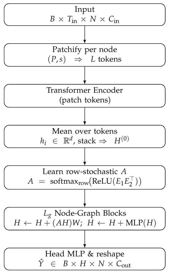
Figure 1. PTSTG overview: patch-level temporal encoding, learned adjacency A, lightweight node-graph refinement, and single-pass multi-horizon head.

3.5. Algorithmic Description

• Notation

The overall training and inference procedure of PTSTG is summarized in Algorithm 1, which outlines the patch-based temporal encoding, adaptive adjacency learning, and graph refinement loop. To highlight the differences between our method and a strong temporal baseline, a direct side-by-side comparison of PatchTST and PTSTG is provided in Table 1.

Table 1. Side-by-side comparison of PatchTST and the proposed PTSTG.

Aspect	PatchTST (Baseline)	PTSTG (Ours)
Input handling	Channel-independent temporal encoder per node/series	Same temporal encoder per node, then node embeddings are refined spatially
Temporal tokens	Fixed-length overlapping patches; positional encodings; Transformer encoder	Identical patching and encoder; outputs pooled to node-level embeddings
Spatial modeling	None explicitly (temporal-only)	Learned row-stochastic adjacency with lightweight node-graph refinement
Adjacency source	Not used	Data-driven, trainable, optionally sparsified at inference
Spatial operation	Not applicable	Linear neighbor aggregation plus position-wise MLP with residuals
Decoder strategy	Single-pass multi-horizon head	Single-pass multi-horizon head (identical usage)
Primary objective	Efficient long-range temporal pattern extraction	Temporal efficiency plus data-driven spatial coupling
Complexity trend	Dominated by patch attention over time	Adds inexpensive cross-node mixing; can use top-k sparsification
Training behavior	Stable optimization via patching	Similarly stable; adjacency learning converges quickly in practice
Inference mode	Single forward pass	Single forward pass; scalable with sparse adjacency
Interpretability	Temporal attention patterns only	Temporal attention and interpretable learned adjacency over nodes

We use P (patch length), s (stride), L (number of patches), d (width), r (graph rank), and $L_g$ (graph depth). Softmax is row-wise unless specified.

Algorithm 1 PTSTG forward pass and training loop

Input:  Training set $\mathcal{D}=\left\{\right(X,Y\left)\right\}$; patch length P; stride s; embedding size d; number of graph layers $L_g$; optimizer Adam; loss $\mathcal{L}$. Output:  Multi-horizon prediction $\widehat{Y}$.   1: Initialize Transformer encoder, projection layers, graph embeddings $E_1, E_2$, graph-block weights $\left\{W_{\mathsf{\ell }}\right\}$, and head.   2: for each minibatch $(X,Y)$ do   3:   Temporal encoding:  for each node i, $U_i\leftarrow \mathcal{P}(X[:,:,i,:];P,s)$; $Z_i\leftarrow \mathrm{TransformerEncoder}\left(\mathrm{LN}(U_i{W}_p+b_p+\mathrm{PE})\right)$; $h_i\leftarrow {\displaystyle \frac{1}{L}}{\sum }_{\mathsf{\ell }}{Z}_{i\mathsf{\ell }}$.   4:    $H^{\left(0\right)}\leftarrow \mathrm{Stack}(h_1,\dots ,h_N)$.   5:    Adaptive adjacency: $S\leftarrow \mathrm{ReLU}\left(E_1{E}_2^{\top }\right)$; $\tilde{S}\leftarrow \frac{1}{2}(S+S^{\top })$; $A\leftarrow {\mathrm{softmax}}_{\mathrm{row}}\left(\tilde{S}\right)$.   6:   Graph refinement: for $\mathsf{\ell }=0,\dots ,L_g-1$: $\widehat{H}\leftarrow H^{(\mathsf{\ell })}+\left(A{H}^{(\mathsf{\ell })}\right)W_{\mathsf{\ell }}$; $\tilde{H}\leftarrow \mathrm{LN}\left(\widehat{H}\right)$; $H^{(\mathsf{\ell }+1)}\leftarrow \tilde{H}+\mathrm{MLP}\left(\tilde{H}\right)$.   7:    Prediction: $\widehat{Y}\leftarrow \mathrm{Reshape}\left({\mathrm{MLP}}_{\mathrm{head}}\left(\mathrm{LN}\left(H^{\left(L_g\right)}\right)\right)\right)$.   8:    Compute $\mathcal{J}=\mathcal{L}(\widehat{Y},Y)$ and update parameters.   9: end for

3.6. Complexity and Practical Considerations

• Computational complexity.

Let $L=\lfloor (T_{\mathrm{in}}-P)/s\rfloor +1$ be the number of patch tokens. One temporal layer costs $\mathcal{O}\left(BN{L}^{2}d\right)$ for self-attention and $\mathcal{O}\left(BNL{d}^2\right)$ for the feed-forward sublayer; the dominant activation memory is $\mathcal{O}\left(BN{L}^{2}d\right)$. Learning the adaptive graph requires an $E_1{E}_2^{\top }$ product of cost $\mathcal{O}\left(N^{2}r\right)$. Each node-graph block costs $\mathcal{O}\left(B{N}^{2}d\right)$ for $\left(AH\right)$ and $\mathcal{O}\left(BN{d}^2\right)$ for its MLP. With row-wise top-k sparsification, the spatial term reduces to $\mathcal{O}\left(BNkd\right)$ and storage $\mathcal{O}\left(Nk\right)$. Empirical efficiency curves (latency, throughput, and peak memory vs. N) will be included in the artifact.

• Training objective.

We use a direct multi-horizon objective,

$$\mathcal{L}(\widehat{Y},Y)=\sum _{t=1}^H{w}_t{\parallel {\widehat{Y}}_{(:,t,:,:)}-Y_{(:,t,:,:)}\parallel }_p,p\in \{1,2\},$$

(15)

with nonnegative weights $w_t$ (uniform unless stated). Optimization choices (optimizer, schedules, and regularization) are orthogonal to the architecture and specified in the experimental section.

• Properties of the learned adjacency.

Row-stochasticity:$A\mathbf{1} = \mathbf{1}$ by construction in (9). Asymmetry: The row-softmax generally breaks symmetry; if needed, symmetric normalization $D^{-1/2}A{D}^{-1/2}$ or Sinkhorn projections can be applied, or mutual top-k selection can enforce symmetric sparsity. Stability: Row-stochastic mixing corresponds to convex combinations of neighbor embeddings and helps numerical stability.

• Implementation notes.

We use pre-norm Transformers with GELU; linear layers are initialized with truncated normal; sinusoidal positional encodings are added before the encoder. Mean pooling over patch tokens is the default; attention pooling is a drop-in replacement under the same interface. For large N, we recommend top-k sparsification of A at train and test time with row re-normalization.

• Exogenous variables.

PTSTG readily accommodates exogenous covariates without architectural changes. Node-wise time-varying features $Z\in {\mathbb{R}}^{B\times T_{\mathrm{in}}\times N\times C_{\mathrm{exo}}}$ (e.g., per-sensor weather or incident flags) can be concatenated with X along the channel dimension and encoded by the same patch encoder. Global covariates $G\in {\mathbb{R}}^{B\times T_{\mathrm{in}}\times C_g}$ (e.g., city-level weather, calendar/event indicators) are projected with a small MLP and broadcast-added to patch tokens; static node attributes $S\in {\mathbb{R}}^{N\times C_s}$ are embedded and added to $H^{\left(0\right)}$. Optionally, these covariates can condition the learned adjacency by FiLM-style modulation of the node-embedding matrices $(E_1, E_2)$ that construct A, enabling context-aware spatial coupling.

• Limitations.

Without sparsification, $\left(AH\right)$ scales quadratically in N. Mean pooling may discard fine-grained temporal cues for highly nonstationary series. The learned A is input-agnostic in this formulation; time-varying graphs and multi-scale patching are compatible extensions but are outside the core design.

• Dynamic (input-conditioned) adjacency.

In the current form, the learned adjacency A is input-agnostic (static across samples), which trades flexibility for stability and efficiency. This may limit the ability to capture regime-dependent spatial couplings (e.g., incidents, rush hours). A natural extension is an input-conditioned graph: produce $A_t$ from the current window by modulating the node-embedding factors $(E_1, E_2)$ with a small hypernetwork $f_{\varphi }$ that summarizes the temporal encoder outputs $\left\{h_i\right\}$:

$$A_t={\mathrm{softmax}}_{\mathrm{row}}\left({\displaystyle \frac{\mathrm{ReLU}\left({\tilde{E}}_1{\tilde{E}}_2^{\top }\right)}{\tau }}\right).$$

(16)

4. Experiments

We evaluate PTSTG on widely used traffic speed benchmarks against strong temporal, graph-based, and hybrid baselines. We report accuracy at short/medium horizons and analyze the effect of patch-based temporal encoding and adaptive adjacency, along with efficiency considerations.

4.1. Datasets

We follow the established protocol of Li et al. [4], Wu et al. [16].

METR–LA. Traffic speed recorded every 5 min by $N=207$ loop detectors in Los Angeles, spanning March–June 2012. Sequences are time-aligned; missing values are imputed by linear interpolation within short gaps and masked when gaps exceed a preset threshold.

PEMS–BAY. Traffic speed from $N=325$ sensors in the Bay Area, sampled every 5 min between January–May 2017. Preprocessing mirrors METR–LA (alignment, short-gap interpolation, masking of long gaps).

LargeST. A large-scale benchmark suite of urban road networks across multiple cities, with tens of thousands of sensors per city and 5-min sampling. It provides standardized train/validation/test splits and graph construction (e.g., geo-kNN) for consistent comparison at scale. We adopt the official splits and evaluation protocol.

All series are standardized (z-score) per node and channel using training statistics only. We use the conventional chronological split of $70\%/10\%/20\%$ into train/validation/test for METR–LA and PEMS–BAY; for LargeST we use the official splits. Unless stated otherwise, we report horizons $\{3,6,12\}$ steps (15, 30, 60 min).

4.2. Evaluation Metrics

We report mean absolute error (MAE) and root mean square error (RMSE). Let $\{{\widehat{y}}_{t,n},y_{t,n}\}$ denote predictions and ground truth for time t and node n, aggregated over all test timestamps $\mathcal{T}$ and nodes $\mathcal{N}$ ($M = \left|\mathcal{T}\right|\left|\mathcal{N}\right|$):

$$\mathrm{MAE}={\displaystyle \frac{1}{M}}\sum _{t\in \mathcal{T}}\sum _{n\in \mathcal{N}}\left|{\widehat{y}}_{t,n}-y_{t,n}\right|,\mathrm{RMSE}=\sqrt{{\displaystyle \frac{1}{M}}{\sum }_{t\in \mathcal{T}}{\sum }_{n\in \mathcal{N}}{\left({\widehat{y}}_{t,n}-y_{t,n}\right)}^2}.$$

(17)

For mean absolute percentage error (MAPE) we clamp the denominator to avoid division by near-zero values (we use $\epsilon =1.0$ in speed units for our runs):

$$\mathrm{MAPE}=100\times {\displaystyle \frac{1}{M}}\sum _{t\in \mathcal{T}}\sum _{n\in \mathcal{N}}\left|{\displaystyle \frac{{\widehat{y}}_{t,n}-y_{t,n}}{max\left(\right|y_{t,n}|,\epsilon )}}\right|.$$

(18)

Because reported baselines often differ in $\epsilon$ and missing-value handling, MAE/RMSE are prioritized for cross-paper comparability, and MAPE is provided for reference only.

4.3. Baselines

We compare against representative methods spanning temporal-only, graph-only, and hybrid spatio–temporal modeling paradigms. When official code is available, we use it with recommended settings; otherwise, we re-implement according to the papers and tune on the validation set.

Classical/temporal baselines. Historical Average (HA), ARIMA (with Kalman filtering), Vector Auto-Regression (VAR), Support Vector Regression (SVR), Feedforward Neural Network (FNN), and FC-LSTM.

Graph spatio–temporal baselines. STGCN [3], DCRNN [4], Graph WaveNet (GWNET) [16], AGCRN [18], GMAN [19], DGCRN [27].

Hybrid/attention baselines. STTN [22], ASTGNN [24], ${\mathrm{D}}^2$STGNN [30], and a channel-independent PatchTST variant [8] as a strong temporal encoder without explicit graph coupling.

This set covers temporal Transformers, fixed-graph and adaptive/dynamic-graph paradigms. On METR–LA and PEMS–BAY we report a representative subset with stable, widely reused baselines to avoid confounding implementation details; a broader set of strong hybrids is included on the large-scale LargeST benchmark. We do not claim strict SOTA across all datasets; instead, we position PTSTG as a compact, competitive alternative with clear headroom under capacity scaling.

4.4. PTSTG Training Setup

Optimization and regularization. We use the Adam optimizer with cosine learning-rate decay and linear warm-up, early stopping on validation MSE, gradient clipping by value, weight decay, and dropout in the feed-forward sublayers. Unless noted, results are single-run point estimates obtained with a fixed random seed (2023). We do not conduct statistical significance tests in this version.

Input/output. A fixed look-back window $T_{\mathrm{in}}$ is fed per node; the model outputs the full horizon H in a single pass. Per-node/channel z-score standardization is fit on training data and inverted at evaluation.

Model configuration. PTSTG comprises a channel-independent patch-based Transformer encoder, a learnable low-rank adaptive adjacency with row-wise temperature $\tau = 1.0$, and a lightweight stack of node graph blocks. Unless stated otherwise, we do not sparsify A during training; at inference we optionally apply top-k row-wise sparsification with re-normalization (we report k when used). The multi-horizon loss in Equation (15) uses uniform weights $w_t = 1$.

4.5. Main Results

• METR–LA.

PTSTG provides competitive MAE/RMSE/MAPE across 15/30/60 min without outperforming the strongest diffusion-based baseline (DCRNN) in our point-estimate runs (Table 2). The gap remains moderate at 15–30 min and increases at 60 min.

Table 2. Performance on METR–LA at 15/30/60 min (lower is better). Baseline values are taken verbatim from the literature(e.g., [4,16]); we did not rerun these baselines. PTSTG values are our single-run point estimates (seed = 2023). Minor discrepancies across publications may stem from preprocessing choices and MAPE conventions ($\epsilon$). Best numbers in bold.

Horizon (T)	Metric	HA	${\mathrm{ARIMA}}_{\mathbf{Kal}}$	VAR	SVR	FNN	FC-LSTM	DCRNN	Ours
15 min	MAE	4.16	3.99	4.42	3.99	3.99	3.44	2.77	2.85
	RMSE	7.80	8.21	7.89	8.45	7.94	6.30	5.38	5.33
	MAPE	13.0%	9.60%	10.2%	9.3%	9.9%	9.6%	7.3%	7.7%
30 min	MAE	4.16	5.15	5.41	5.05	4.23	3.77	3.15	3.39
	RMSE	7.80	10.45	9.13	10.87	8.17	7.23	6.45	6.41
	MAPE	13.0%	12.7%	12.7%	12.1%	12.9%	10.9%	8.8%	9.7%
1 h	MAE	4.16	6.90	6.52	6.72	4.49	4.37	3.60	4.19
	RMSE	7.80	13.23	10.11	13.76	8.69	8.69	7.59	7.69
	MAPE	13.0%	17.4%	15.8%	16.7%	14.0%	13.2%	10.5%	12.67%

• PEMS–BAY.

A similar pattern holds: PTSTG is competitive among recent graph–temporal models but does not surpass the strongest baseline (Table 3). Short-horizon differences are small, while the one-hour horizon exhibits a larger margin.

Table 3. Performance on PEMS–BAY at 15/30/60 min (lower is better). Baseline values are taken verbatim from the literature (e.g., [4,16]); we did not rerun these baselines. PTSTG values are our single-run point estimates (seed = 2023). Due to heterogeneous MAPE definitions in prior work, MAE/RMSE should be taken as the primary basis for comparison. Best numbers in bold.

Horizon (T)	Metric	HA	${\mathrm{ARIMA}}_{\mathbf{Kal}}$	VAR	SVR	FNN	FC-LSTM	DCRNN	Ours
15 min	MAE	2.88	1.62	1.74	1.85	2.20	2.05	1.38	1.55
	RMSE	5.59	3.30	3.16	3.59	4.42	4.19	2.95	3.12
	MAPE	6.8%	3.5%	3.6%	3.8%	5.19%	4.8%	2.9%	3.43%
30 min	MAE	2.88	2.33	2.32	2.48	2.30	2.20	1.74	2.08
	RMSE	5.59	4.76	4.25	5.18	4.63	4.55	3.97	4.28
	MAPE	6.8%	5.4%	5.0%	5.5%	5.43%	5.2%	3.90%	4.84%
1 h	MAE	2.88	3.38	2.93	3.28	2.46	2.37	2.07	2.81
	RMSE	5.59	6.50	5.44	7.08	4.98	4.96	4.74	5.54
	MAPE	6.8%	8.3%	6.50%	8.0%	5.89%	5.7%	4.90%	6.81%

• LargeST.

On a large-scale city network, PTSTG achieves favorable average RMSE/MAE and a compact parameterization (Table 4). It remains behind the top hybrid (e.g., ${\mathrm{D}}^2$STGNN) on some individual horizons, but attains competitive average performance and efficiency.

Table 4. Results on the LargeST benchmark (SD) with horizons $\{3, 6, 12\}$ (lower is better). Baseline values are taken verbatim from official LargeST reports and follow-up papers (e.g., [31] for ${\mathrm{D}}^2$STGNN); we did not rerun these baselines. PTSTG values are our single-run point estimates (seed = 2023). Numbers can vary across city coverage, graph construction, and MAPE denominator clamping. Best numbers in bold.

Method	Param	Horizon 3				Horizon 6				Horizon 12				Average
		MAE	RMSE	MAPE		MAE	RMSE	MAPE		MAE	RMSE	MAPE		MAE	RMSE	MAPE
HL	–	33.61	50.97	20.77%		57.80	84.92	37.73%		101.74	140.14	76.84%		60.79	87.40	41.88%
LSTM	98K	19.03	30.53	11.81%		25.84	40.87	16.44%		37.63	59.07	25.45%		26.44	41.73	17.20%
DCRNN	373K	17.14	27.47	11.12%		20.99	33.29	13.95%		26.99	42.86	18.67%		21.03	33.37	14.13%
AGCRN	761K	15.71	27.85	11.48%		18.06	31.51	13.06%		21.86	39.44	16.52%		18.09	32.01	13.28%
STGCN	508K	17.45	29.99	12.42%		19.55	33.69	13.68%		23.21	41.23	16.32%		19.67	34.14	13.86%
GWNET	311K	15.24	25.13	9.86%		17.74	29.51	11.70%		21.56	36.82	15.13%		17.74	29.62	11.88%
ASTGCN	2.2M	19.56	31.33	12.18%		24.13	37.95	15.38%		30.96	49.17	21.98%		23.70	37.63	15.65%
STTN	114K	16.22	26.22	10.63%		18.76	30.98	12.80%		22.62	39.09	16.14%		18.69	31.11	12.82%
STGODE	729K	16.75	28.04	11.00%		19.71	33.56	13.16%		23.67	42.12	16.58%		19.55	33.57	13.22%
DSTAGNN	3.9M	18.13	28.96	11.38%		21.71	34.44	13.93%		27.51	43.95	19.34%		21.82	34.68	14.40%
DGCRN	243K	15.34	25.35	10.01%		18.05	30.06	11.90%		22.06	37.51	15.27%		18.02	30.09	12.07%
${\mathrm{D}}^2$STGNN	406K	14.92	24.95	9.56%		17.52	29.24	11.36%		22.62	37.14	14.86%		17.85	29.51	11.54%
Ours	880K	16.42	26.42	11.04%		18.86	30.37	12.93%		22.69	36.42	16.59%		17.50	28.18	11.07%

As summarized in Table 5, PTSTG demonstrates its computational footprint on a single consumer GPU.

Table 5. PTSTG computational footprint on a single consumer GPU. Hardware: NVIDIA GeForce RTX 4060 Ti (8 GB), FP32; PyTorch v2.8.0 setup as in Section 4.7. Input: batch $B=32$, $\mathrm{Seq}\text{\_}\mathrm{len}=36$, $\mathrm{Horizon}=12$. FLOPs are per forward pass at $B=1$; latency/throughput(THPT) are per mini-batch ($B=32$).

Model	Params (M)	FLOPs (G)	Train/Epoch (min)	Infer Mean (ms)	Infer p95 (ms)	THPT (seq/s)	Peak VRAM (GB)
PTSTG (ours)	0.88	119.163	3.101	56.44	61.54	564.04	3.492

4.6. Ablations and Efficiency

We qualitatively assess three design choices—(i) patch tokens vs. step-wise tokens, (ii) learned vs. fixed-distance adjacency, and (iii) graph depth $L_g$. In our experiments, patching stabilized optimization and improved short/medium-range accuracy; learned adjacency consistently outperformed a distance kNN graph; and increasing $L_g$ benefited 30–60 min horizons. Numeric ablations (no-patch vs. patch; learned-A vs. distance-A vs. none; sweeps over $L_g$ and graph rank; sensitivity to top-k) and efficiency profiles (latency/throughput/VRAM at $N\in \{200, 1\mathrm{k}, 10\mathrm{k}\}$) will be released with the public artifact to ensure exact reproducibility without space constraints.

4.7. Implementation Details

PTSTG is implemented in PyTorch. We standardize each node/channel with z-scores computed on the training split and invert the transform at evaluation. Models are trained with Adam optimizer, cosine learning-rate decay with linear warm-up, early stopping on validation MSE, gradient clipping by value, dropout in the feed-forward sublayers, and weight decay. The model consumes a fixed look-back window ($\mathrm{Seq}\text{\_}\mathrm{len}$) and outputs the full horizon (Horizon) in a single pass. All experiments use a 5-min sampling step. Exact training/optimization and architectural hyperparameters per dataset are given in Table 6 and Table 7.

Table 6. Training and optimization hyperparameters for PTSTG. $\mathrm{Seq}\text{\_}\mathrm{len}$ is the look-back window in 5-min steps; Horizon is the prediction length in steps.

Dataset	Seq_len	Horizon	Step	Batch	MaxEp	Pat.	LR	WD	GradClip	Dropout	Loss	Seed
METR–LA	36	12	5 min	32	50	5	$1 \times {10}^{-4}$	$1 \times {10}^{-3}$	5.0	0.30	MSE	2023
PEMS–BAY	36	12	5 min	64	50	5	$1 \times {10}^{-4}$	$1 \times {10}^{-3}$	5.0	0.30	MSE	2023
LargeST (SD)	36	12	5 min	32	50	5	$1 \times {10}^{-4}$	$1 \times {10}^{-3}$	5.0	0.30	MSE	2023

Table 7. Architectural hyperparameters of PTSTG. $d_{\mathrm{model}}$ is the embedding width; n_heads/n_layers refer to the PatchTST encoder; patch_len/stride defines temporal tokenization; graph_rank parameterizes the low-rank adaptive adjacency; graph_layers is the number of node-graph blocks.

Dataset	${\mathit{d}}_{\mathbf{model}}$	n_heads	n_layers	patch_len	stride	graph_rank	graph_layers	Input_dim	Output_dim	Dropout
METR–LA	128	4	2	8	4	12	3	1	1	0.30
PEMS–BAY	128	4	2	12	6	16	3	1	1	0.30
LargeST (SD)	128	4	2	8	4	12	3	1	1	0.30

• Reporting choices and protocol clarifications.

MAPE is computed on de-normalized speeds with a denominator clamp $\epsilon =1.0$ (speed unit) to avoid division by near-zero values. Row-wise softmax temperature for the learned adjacency is $\tau =1$. Unless stated otherwise, no top-k sparsification is applied to A during training or evaluation in the reported numbers (i.e., k is not used). Missing values are linearly interpolated within short gaps and masked when gaps exceed a predefined threshold, following prior work.

• Statistical reporting.

All reported numbers are single-run point estimates with a fixed random seed (2023) under a unified training/evaluation protocol. While multi-seed reporting (mean ± std) is preferable, it was beyond our computing budget for this manuscript. To facilitate replication, we release training scripts and configs that support multi-seed runs out-of-the-box; future work will include aggregated statistics.

• Reproducibility and artifact availability.

All code and configuration files needed to reproduce our experiments are publicly available at https://github.com/mtuciru/PTSTG (accessed on 23 September 2025).

Societal and Deployment Considerations

Fairness across road types and regions. Model errors can vary systematically across functional classes (e.g., freeways vs. arterials) and neighborhoods. To avoid reinforcing inequities (e.g., systematically worse travel-time estimates on minor roads), we recommend stratified evaluation by road class and district, reporting per-stratum MAE/RMSE and gap metrics, and rebalancing training where harmful gaps are observed.

Robustness to sensor failures and missing data. Real-world networks exhibit outages, drift, and asynchronous timestamps. Although PTSTG tolerates short gaps via interpolation and masking, deployment should include robustness tests that randomly mask nodes/intervals at inference time, impute with model-based or graph-aware methods, and maintain fallbacks (historical profiles, neighbor-based heuristics) when coverage drops.

Distribution shift and incidents. The learned, input-agnostic adjacency may encode spurious correlations and under-react to regime shifts (incidents, events, weather). Mitigations include regularization and sparsification of A, periodic retraining with recent data, input-conditioned or time-varying graphs, explicit exogenous covariates, and online monitoring of calibration and error drift.

Interpretability and accountability. While row-stochastic A is amenable to inspection, links need not correspond to physical roads. We advocate publishing qualitative audits (e.g., top-k neighbors per node with geographic overlays) and documenting changes to A over time to support operator review.

5. Conclusions

We introduced PTSTG, a compact hybrid forecaster that combines a PatchTST-style, channel-independent temporal encoder with a learned row-stochastic adjacency and a small stack of node-graph refinement blocks. The model performs single-pass, multi-horizon decoding and cleanly separates temporal tokenization from spatial aggregation. Across METR–LA, PEMS–BAY, and LargeST (SD), PTSTG delivers competitive accuracy while emphasizing efficiency (short-attention over patch tokens, no auto-regressive rollout), compactness, and scalability to large sensor sets. Capacity sweeps indicate predictable gains with modest increases in embedding width and graph depth, suggesting headroom without changing the architecture.

Our contribution is positioned primarily in terms of practical trade-offs rather than universal accuracy dominance: PTSTG offers a lightweight temporal path, a data-driven spatial coupling that avoids fixed topologies, and a restrained parameter budget that accelerates training and reduces memory usage. Limitations remain. Dense inter-node mixing scales quadratically with the number of sensors (mitigated by top-k sparsification). The learned adjacency is currently input-agnostic and may under-react to sudden regime shifts. Mean pooling over patch tokens can lose fine-grained temporal detail in highly non-stationary segments.

Regarding future work vis-à-vis existing literature, several themes are related but distinct in scope. Multi-scale temporal modeling has been explored via decomposition/frequency designs (e.g., Autoformer, FEDformer, ETSformer, Crossformer) [7,9,10,12]; our aim is a PatchTST-native multi-scale tokenization (short/long patches in parallel) that reuses the same lightweight learned graph, with scale-specific pooling and a minimal cross-scale gating head to preserve the model’s simplicity. For dynamic spatial relations, prior dynamic/adaptive graphs exist (e.g., Graph WaveNet, AGCRN, DGCRN) [16,18,27]; our extension will keep the row-stochastic parameterization but modulate it with low-cost, input-conditioned factors (e.g., a small hypernetwork) to maintain efficiency. Finally, we plan to incorporate exogenous variables (weather, calendar/events, incidents) through additive or cross-attention side paths that feed both the temporal encoder and the graph learner, and to provide uncertainty estimates via lightweight distributional heads or ensembling. Together, these steps target improved robustness and interpretability while retaining PTSTG’s core advantages in efficiency and deployability for intelligent transportation systems.

References

- Hochreiter, S.; Schmidhuber, J. Long Short-Term Memory. Neural Comput. 1997, 9, 1735–1780. [Google Scholar] [CrossRef] [PubMed]
- Cho, K.; van Merriënboer, B.; Gulcehre, C.; Bahdanau, D.; Bougares, F.; Schwenk, H.; Bengio, Y. Learning phrase representations using RNN encoder–decoder for statistical machine translation. In Proceedings of the Conference on Empirical Methods in Natural Language Processing (EMNLP), Doha, Qatar, 25–29 October 2014; pp. 1724–1734. [Google Scholar]
- Yu, B.; Yin, H.; Zhu, Z. Spatio-Temporal Graph Convolutional Networks: A Deep Learning Framework for Traffic Forecasting. In Proceedings of the Twenty-Seventh International Joint Conference on Artificial Intelligence (IJCAI-2018), Stockholm, Sweden, 13–19 July 2018; pp. 3634–3640. [Google Scholar] [CrossRef]
- Li, Y.; Yu, R.; Shahabi, C.; Liu, Y. Diffusion Convolutional Recurrent Neural Network: Data-Driven Traffic Forecasting. arXiv 2017, arXiv:1707.01926. [Google Scholar]
- Vaswani, A.; Shazeer, N.; Parmar, N.; Uszkoreit, J.; Jones, L.; Gomez, A.N.; Kaiser, L.; Polosukhin, I. Attention is all you need. arXiv 2017, arXiv:1706.03762. [Google Scholar]
- Zhou, H.; Zhang, S.; Peng, J.; Zhang, S.; Li, J.; Xiong, J.; Xiong, Z.; Zhang, W. Informer: Beyond Efficient Transformer for Long Sequence Time-Series Forecasting. In Proceedings of the AAAI Conference on Artificial Intelligence, Vancouver, BC, Canada, 2–9 February 2021; Volume 35, pp. 11106–11115. [Google Scholar]
- Wu, H.; Xu, J.; Wang, J.; Long, M.; Jiang, J.; Wang, C. Autoformer: Decomposition Transformers with Auto-Correlation for Long-Term Series Forecasting. In Proceedings of the Advances in Neural Information Processing Systems 34 (NeurIPS 2021), Online, 6–14 December 2021; Volume 34, pp. 22419–22430. [Google Scholar]
- Nie, Y.; Nguyen, N.H.; Sinthong, P.; Kalagnanam, J. A Time Series is Worth 64 Words: Long-Term Forecasting with Transformers. arXiv 2022, arXiv:2211.14730. [Google Scholar]
- Zhou, T.; Ma, Z.; Wen, Q.; Wang, X.; Sun, L.; Jin, R. FEDformer: Frequency Enhanced Decomposed Transformer for Long-Term Series Forecasting. In Proceedings of the International Conference on Machine Learning (ICML), Baltimore, MD, USA, 17–23 July 2022; pp. 27268–27286. [Google Scholar]
- Zhang, Y.; Yan, J. Crossformer: Transformer Utilizing Cross-Dimension Dependency for Multivariate Time Series Forecasting. In Proceedings of the International Conference on Learning Representations (ICLR), Kigali, Rwanda, 1–5 May 2023. [Google Scholar]
- Liu, D.; Zhou, H.; Wu, J.; Deng, W.; Chen, W.; Zhang, C.; Ma, Z.; Sun, L. Non-stationary Transformers: Exploring the Stationarity in Time Series Forecasting. In Proceedings of the International Conference on Learning Representations (ICLR), Virtual, 25 April 2022. [Google Scholar]
- Woo, G.; Liu, C.; Sahoo, D.; Kumar, A.; Hoi, S.C. ETSformer: Exponential Smoothing Transformers for Time-Series Forecasting. arXiv 2022, arXiv:2202.01381. [Google Scholar] [CrossRef]
- Zeng, A.; Chen, M.; Zhang, L.; Xu, Q.; Yu, Y.; Wang, L. Are Transformers Effective for Time Series Forecasting? In Proceedings of the AAAI Conference on Artificial Intelligence, Washington, DC, USA, 7–14 February 2023; Volume 37, pp. 14800–14808. [Google Scholar]
- Yu, C.; Lin, H.; Dong, W.; Fang, S.; Yuan, Q.; Yang, C. TripChain2RecDeepSurv: A Novel Framework to Predict Transit Users’ Lifecycle Behavior Status Transitions for User Management. Transp. Res. Part C Emerg. Technol. 2024, 167, 104818. [Google Scholar] [CrossRef]
- Song, C.; Lin, Y.; Guo, S.; Wan, H. Spatial-Temporal Synchronous Graph Convolutional Networks: A New Framework for Spatial-Temporal Network Data Forecasting. In Proceedings of the AAAI Conference on Artificial Intelligence, New York, NY, USA, 7–12 February 2020; Volume 34, pp. 914–921. [Google Scholar]
- Wu, Z.; Pan, S.; Long, G.; Jiang, J.; Chang, X.; Zhang, C. Graph WaveNet for Deep Spatial-Temporal Graph Modeling. In Proceedings of the International Joint Conference on Artificial Intelligence (IJCAI), Macao, China, 10–16 August 2019; pp. 1907–1913. [Google Scholar]
- Wu, Z.; Pan, S.; Long, G.; Jiang, J.; Chang, X.; Zhang, C. Connecting the Dots: Multivariate Time Series Forecasting with Graph Neural Networks. In Proceedings of the 26th ACM SIGKDD Conference on Knowledge Discovery and Data Mining, Virtual, 6–10 July 2020; pp. 753–763. [Google Scholar]
- Bai, L.; Yao, L.; Li, C.; Wang, X.; Wang, C. Adaptive Graph Convolutional Recurrent Network for Traffic Forecasting. In Proceedings of the Annual Conference on Neural Information Processing Systems 2020 (NeurIPS 2020), Virtual, 6–12 December 2020; Volume 33, pp. 17804–17815. [Google Scholar]
- Zheng, C.; Fan, X.; Wang, C.; Qi, J. GMAN: A Graph Multi-Attention Network for Traffic Prediction. In Proceedings of the AAAI Conference on Artificial Intelligence, New York, NY, USA, 7–12 February 2020; Volume 34, pp. 1234–1241. [Google Scholar]
- Cao, D.; Wang, Y.; Li, J.; Zhou, H.; Li, L. Spectral Temporal Graph Neural Network for Multivariate Time-Series Forecasting. In Proceedings of the Annual Conference on Neural Information Processing Systems 2020 (NeurIPS 2020), Virtual, 6–12 December 2020; Volume 33, pp. 17766–17778. [Google Scholar]
- Grigsby, J.; Wang, Z.; Nguyen, N.H.; Qi, Y. Long-Range Transformers for Dynamic Spatiotemporal Forecasting. arXiv 2021, arXiv:2109.12218. [Google Scholar]
- Xu, K.; Liu, X.; Zheng, H.; Guan, H. Spatial-Temporal Transformer Networks for Traffic Flow Forecasting. arXiv 2020, arXiv:2001.02908. [Google Scholar]
- Feng, A.; Tassiulas, L. Adaptive Graph Spatial-Temporal Transformer Network for Traffic Flow Forecasting. In Proceedings of the 31st ACM International Conference on Information and Knowledge Management (CIKM), Atlanta, GA, USA, 17–21 October 2022; pp. 3933–3937. [Google Scholar]
- Guo, S.; Lin, Y.; Wan, H.; Li, X.; Cong, G. Attention Based Spatio-Temporal Graph Neural Network for Traffic Forecasting. IEEE Trans. Knowl. Data Eng. 2021, 34, 5415–5428. [Google Scholar] [CrossRef]
- Liu, H.; Dong, Z.; Jiang, R.; Deng, J.; Chen, Q.; Song, X. STAEformer: Spatio-Temporal Adaptive Embedding Makes Vanilla Transformer SOTA for Traffic Forecasting. In Proceedings of the 32nd ACM International Conference on Information and Knowledge Management, Birmingham, UK, 21–25 October 2023. [Google Scholar]
- Zhou, J.; Liu, E.; Chen, W.; Zhong, S.; Liang, Y. Navigating Spatio-Temporal Heterogeneity: A Graph Transformer Approach for Traffic Forecasting. arXiv 2024, arXiv:2408.10822. [Google Scholar] [CrossRef]
- Li, F.; Wu, J.; Xu, J.; Long, M.; He, D. Dynamic Graph Convolutional Recurrent Network for Traffic Prediction: Benchmark and Solution. ACM Trans. Knowl. Discov. Data 2023, 17, 1–21. [Google Scholar] [CrossRef]
- Shang, C.; Chen, J.; Bi, J. Discrete Graph Structure Learning for Forecasting Multiple Time Series. arXiv 2021, arXiv:2101.06861. [Google Scholar] [CrossRef]
- Li, M.; Zhu, Z. Spatial-Temporal Fusion Graph Neural Networks for Traffic Flow Forecasting. In Proceedings of the AAAI Conference on Artificial Intelligence, Virtual, 2–9 February 2021; Volume 35, pp. 4189–4196. [Google Scholar]
- Shao, Z.; Zhang, Z.; Wei, W.; Wang, F.; Xu, Y.; Cao, X.; Jensen, C.S. Decoupled Dynamic Spatial-Temporal Graph Neural Network for Traffic Forecasting. Proc. Vldb Endow. (PVLDB) 2022, 15, 2733–2746. [Google Scholar] [CrossRef]
- Fang, Y.; Liang, Y.; Hui, B.; Shao, Z.; Deng, L.; Liu, X.; Jiang, X.; Zheng, K. Efficient Large-Scale Traffic Forecasting with Transformers: A Spatial Data Management Perspective. In Proceedings of the 31st ACM SIGKDD Conference on Knowledge Discovery and Data Mining, Toronto, ON, Canada, 3–7 August 2025. [Google Scholar]
Disclaimer/Publisher’s Note: The statements, opinions and data contained in all publications are solely those of the individual author(s) and contributor(s) and not of MDPI and/or the editor(s). MDPI and/or the editor(s) disclaim responsibility for any injury to people or property resulting from any ideas, methods, instructions or products referred to in the content. |
© 2025 by the authors. Licensee MDPI, Basel, Switzerland. This article is an open access article distributed under the terms and conditions of the Creative Commons Attribution (CC BY) license (https://creativecommons.org/licenses/by/4.0/).