Uncertainty Propagation for Vibrometry-Based Acoustic Predictions Using Gaussian Process Regression

Abstract

Shell-like housing structures for motors and compressors can be found in everyday products. Consumers significantly evaluate acoustic emissions during the first usage of products. Unpleasant sounds may raise concerns and cause complaints to be issued. A prevention strategy is a holistic acoustic design, which includes predicting the emitted sound power as part of end-of-line testing. The hybrid experimental-simulative sound power prediction based on laser scanning vibrometry (LSV) is ideal in acoustically harsh production environments. However, conducting vibroacoustic testing with laser scanning vibrometry is time-consuming, making it difficult to fit into the production cycle time. This contribution discusses how the time-consuming sampling process can be accelerated to estimate the radiated sound power, utilizing adaptive sampling. The goal is to predict the acoustic signature and its uncertainty from surface velocity data in seconds. Fulfilling this goal will enable integration into a product assembly unit and final acoustic quality control without the need for an acoustic chamber. The Gaussian process regression based on PyTorch 2.6.0 performed 60 times faster than the preliminary reference implementation, resulting in a regression estimation time of approximately one second for each frequency bin. In combination with the Equivalent Radiated Power prediction of the sound power, a statistical measure is available, indicating how the uncertainty of a limited number of surface velocity measurement points leads to predictions of the uncertainty inside the acoustical signal. An adaptive sampling algorithm reduces the prediction uncertainty in real-time during measurement. The method enables on-the-fly error analysis in production, assessing the risk of violating agreed-upon acoustic sound power thresholds, and thus provides valuable feedback to the product design units.

1. Introduction

Quantifying the sound generation of highly integrated products is essential during design and production. The overall goal is to enhance product quality and meet contractual and legal requirements. For any device with direct user interaction, noise emissions can negatively affect both the user and the user’s environment [1]. Therefore, tools [2] to predict and quantify sound emissions should be integrated early in the design process and aligned with production-ready methods for quality control and production-based design feedback [3]. A production-ready system for acoustic end-of-line testing to meet vibroacoustic requirements is presented in [4]. Ref. [4] requires an acoustically treated environment for accurate sound measures, whereas the used acoustic measurement method [5] does not rely on a specific treatment of the acoustics in the production facility.

We identify the following specifications of the system [4]: firstly (specification 1), the system should be ready to perform measurements at different locations, contactless, and without any additional assembly cost, in a harsh acoustic environment such as a production facility. Secondly (specification 2), the system should select observation points based on the data prediction accuracy and uncertainty calculated by a self-learned data-driven method. Thirdly (specification 3), the technique should provide data that gives the maximum valuable insight into specific characteristics where the deviations occurred over time. Fourthly and finally (specification 4), the measurement time should align with the production cycle of a production line and the performance test of the end test before delivery.

The objective of the work is to establish an acoustic measurement technique for acoustic end-of-line testing that fulfills system specification 1 and 2, and establish the necessary pre-conditions for system specification 3 and 4. The development of experimental sound prediction methods with far-field prediction based on the boundary element method (BEM) was found to provide accurate results even in non-favorable acoustic environments [5] (realizing specification 1 through being contactless). This method is well-suited to fulfill specification two by utilizing data-driven mapping techniques, such as Gaussian process regression (GPR) [6], to minimize the overall uncertainty of the sound prediction method [7]. The benefit of using GPR is a direct estimate of the uncertainty quantification and risk estimation of exceeding limits is possible [8]. For instance, the next best training points are collected based on where the data is most likely to be the most informative. This Bayesian optimization strategy [9,10] is beneficial in situations where data acquisition is costly or slow, and can improve convergence. It is an iterative search (adaptive) of the next best sampling point based on previous samples. The sampling is updated to focus on areas of the input space that are expected to yield the most significant improvement of the model [11].

In the data acquisition process of surface motion data, GPR was used in various applications of robotics and biomechanics [12,13,14], including real-time [15,16]. In general, the main advantage of GPR over other existing interpolation methods is that it provides a maximum of information of the statistical description from the given data [11,17]. This maximum information gain is well-suited to the stated specifications in the introduction and can further benefit from the sequential design of experiments. However, specification 4 represents a significant obstacle in industrial integration for acoustic testing. Therefore, the contribution of this publication is that it presents the first application of GPR-based uncertainty predictions in vibroacoustics based on descriptive statistics and it discusses the potential speed-up of the Monte Carlo simulation method used in [7]. Firstly, the sampling will be discussed, starting with a minimum number of sampling points and then iteratively refining the number of sampling points. Secondly, the GPR routine of GPyTorch [18] will significantly improve the training and prediction speed of the GPR while continuously updating the model. Thirdly, the far-field prediction will be replaced by the low-fidelity and rapid Equivalent Radiated Power (ERP) method, which is known to be as accurate as the boundary element method (BEM) for high frequencies. Based on the uncertainty estimates from the GPR of the surface velocity, uncertainty in the resulting acoustic signal can be described by the ERP method presented in this work. The usage of BEM would require either the eigenvalues of the correlation matrix of the data points or a Monte Carlo Simulation [19].

In [20], the GPR was performed using scikit-learn 1.6.1 [21], considering 30 restarts to guarantee a robust minimum of the marginal log likelihood cost function. Therewith, at each frequency step (for 32 frequencies), an independent GPR was fitted separately to both the real and imaginary parts of the surface normal velocity frequency response. For each frequency step, 2 GPRs were trained, and restarted 30 times, for 128 sampling points. Subsequently, the two converged GPRs were evaluated using a Monte Carlo method 100 times to compute the mean of the radiated sound power at each vibration frequency. The computation of the radiated sound power was performed using three-dimensional conventional collocational BEM using the Burton–Miller method. The total sound power (BEM) estimation time of this computation was composed of 188.6 s for the GPR training (in total 2 × 32, 64 GPR were executed), 1072 s for drawing the Monte Carlo samples (in total 2 × 32 × 100, 6400 samples were drawn) and 387.9 s to evaluate the BEM (in total 32 BEM systems were solved and 100 × 32 BEM result calculations were performed) on the reference machine (2× Intel Xeon G 5218-16 cores, Intel, Santa Clara, CA, USA). All three steps (GPR training, sample drawing, and the BEM simulations) consume a significant amount of time and consume a large fraction of the process time. In this article, statistical measures for the sound power uncertainty are derived, the speed-up potential of the workflow is discussed, and an adaptive refinement scheme to reduce the uncertainty in the predicted sound power is presented. To show the accuracy of the uncertainty propagation, the statistical sampling is compared to a Monte Carlo (BEM)-simulated reference acoustic prediction.

In summary, integrating GPR into the experimental sound field estimation provides a new perspective on assessing surface vibration measurements for acoustical quantification. In Section 2.1, the GPR details are discussed. Section 3 describes the experimental sound field estimation using laser scanning Doppler vibrometry (LSV). It is followed by the results Section 5, which reports the accuracy, performance, and adaptive refinement procedure of the proposed workflow. Concluding remarks are given in Section 6.

2. Methodology

Figure 1 depicts the proposed workflow schematically. It is based on the workflow presented in [5], where the boundary element method (BEM) was used to predict the radiated sound field based on the structural dynamic. At first, the surface velocity will be obtained from a region of interest (ROI) by data acquisition at a limited number of probing locations, by means of e.g., Laser Scanning Vibrometry (LSV) and Finite Element (FE) simulation. The data is then mapped by a standard interpolation technique [5] or Gaussian process regression (GPR) [20] onto the geometry and the evaluation points for the sound power prediction. Finally, the sound propagation is simulated. The radiated sound field can be predicted in various ways, such as using finite element method, BEM, or comparably fast low-fidelity methods. In this work, GPR is used on a dataset at given sample points to obtain a statistical description of the normal velocity field on the whole structure. Therewith, a statistical description of the sound emission based on the Equivalent Radiated Power (ERP) is computed based on either the Monte Carlo method or direct evaluation as proposed in Section 2.4. The statistical description of the ERP can then be used to assess the quality of the prediction and, finally, additional sample points can be defined in an adaptive refinement step based on an expected improvement function as described in Section 2.5.

2.1. Interpolation Based on Gaussian Process Regression

In this article, the Gaussian process regression (GPR) is selected as an interpolation technique to provide both a mean and an uncertainty quantification [22] of the underlying physical process. If it cannot explain the data, the GPR has a noise level that increases, which may be used as an indication of such an event. It is known to reconstruct statistical distributions from noisy observations without overfitting [23], making it an ideal method for this experimental sound power estimate. The output is modeled at different input points with a mean and a covariance function. It has cubic complexity $O\left(n^3\right)$ in terms of the input data points n, which limits its application to large datasets. As a consequence, a variational Gaussian process is chosen to reduce the computational complexity [24,25] based on approximate inference [26]. The radial basis function (RBF) kernels are a valid choice for a spatially decreasing correlation and may improve the computational speed due to the sparsity of the correlation function. In [20], the complex-valued normal surface velocity ${\mathit{v}}_{\mathrm{s}}·\mathit{n}:=v_{\mathrm{n}}\left(\mathit{x}\right)$ was expressed as Gaussian processes (GP) $v_{\mathrm{n}}\sim \mathcal{GP}\left\{\mu ,k\right\}$ for both real and imaginary part. Sampling this distribution of functions, this results in the Gaussian vector

$$\begin{array}{c}\hfill {\mathit{v}}_{\mathrm{n}}\sim \mathcal{GP}\left\{\mathsf{\mu },\mathit{K}\right\}.\end{array}$$

(1)

where $\mathsf{\mu }:=\mu \left(\mathit{x}\right)$ defines the GP’s mean and $\mathit{K}:=\mathrm{cov}\left(\mathit{x},{\mathit{x}}^{\prime },\mathsf{\theta }\right)$ the covariance matrix, with $\mathsf{\theta }$ denoting hyper-parameters. The radial basis kernel function used to evaluate the covariance matrix reads

$$\begin{array}{c}\hfill \mathit{K}={\sigma }_x^{2}exp\left(-{\displaystyle \frac{1}{2}}\sum _{j=1}^d{\displaystyle \frac{{∥\mathit{d}∥}_2^2}{l^2}}\right).\end{array}$$

(2)

Here, $\mathit{d}=\mathit{x}-{\mathit{x}}^{\prime }$ is the distance vector, l length scale of the automatic relevance determination (ARD) for adjustable length scales for different input dimensions d [27], and ${\sigma }_x^2$ is a gain parameter. The hyperparameters $\mathsf{\theta }$ of the Gaussian process are adapted by optimization to minimize the negative log marginal likelihood objective function $L(\mathit{y},\mathsf{\theta })$ [28]

$$\begin{array}{c}\hfill \underset{\mathsf{\theta }}{\mathrm{argmin}}\left\{-logL(\mathit{v},\mathsf{\theta })\right\}\end{array}$$

(3)

from an initial prior distribution (zero-mean Gaussian process $\sim \mathcal{N}\left(\mathbf{0},\mathit{K}\right)$). Thereafter, the interpolation operation using GPR can be performed by making a prediction ${\mathit{v}}_{\mathrm{n}}^{\ast }$ at location ${\mathit{x}}^{\ast }$ based on the set of training data ${\mathit{v}}_{\mathrm{n}}$ at $\mathit{x}$ as described in [28]. The joint distribution reads

$$\left[\begin{array}{c}{\mathit{v}}_{\mathrm{n}}\\ {\mathit{v}}_{\mathrm{n}}^{\ast }\end{array}\right]\sim \mathcal{N}\left(\left[\begin{array}{c}\mathsf{\mu }\left(\mathit{x}\right)\\ \mathsf{\mu }\left({\mathit{x}}^{\ast }\right)\end{array}\right],\left[\begin{array}{cc}\mathit{K}(\mathit{x},\mathit{x})+{\sigma }_{\ast }^2\mathit{I}& \mathit{K}(\mathit{x},{\mathit{x}}^{\ast })\\ \mathit{K}({\mathit{x}}^{\ast },\mathit{x})& \mathit{K}({\mathit{x}}^{\ast },{\mathit{x}}^{\ast })\end{array}\right]\right)$$

(4)

with the predictive uncertainty ${\sigma }_{\ast }^2$ and leads to the predictive equation

$$\begin{array}{cc}\hfill {\mathit{v}}_{\mathrm{n}}^{\ast }\sim \mathcal{N}& \left(\mathsf{\mu }\left({\mathit{x}}^{\ast }\right)+\mathit{K}({\mathit{x}}^{\ast },\mathit{x}){\left[\mathit{K}(\mathit{x},\mathit{x})+{\sigma }_{\ast }^2\mathit{I}\right]}^{-1}\left[{\mathit{v}}_{\mathrm{n}}-\mathsf{\mu }\left(\mathit{x}\right)\right],\right.\hfill \\ & \left.\mathit{K}({\mathit{x}}^{\ast },{\mathit{x}}^{\ast })-\mathit{K}({\mathit{x}}^{\ast },\mathit{x}){\left[\mathit{K}(\mathit{x},\mathit{x})+{\sigma }_{\ast }^2\mathit{I}\right]}^{-1}\mathit{K}(\mathit{x},{\mathit{x}}^{\ast })\right).\hfill \end{array}$$

(5)

Typically, to improve the condition of the numerical optimization, the input and output data are normalized independently. The mean of the training data ${\mu }_{\mathrm{scaler}}$ is subtracted and it is scaled to unit variance by $X={\displaystyle \frac{x-{\mu }_{\mathrm{scaler}}}{{\sigma }_{\mathrm{scaler}}}}$. Consequently, due to $E\left({\displaystyle \frac{X-{\mu }_{\mathrm{scaler}}}{{\sigma }_{\mathrm{scaler}}}}\right)={\displaystyle \frac{E\left(X\right)-{\mu }_{\mathrm{scaler}}}{{\sigma }_{\mathrm{scaler}}}}$ and $COV\left({\displaystyle \frac{X-{\mu }_{\mathrm{scaler}}}{{\sigma }_{\mathrm{scaler}}}}\right)={\displaystyle \frac{COV\left(X\right)}{{\sigma }_{\mathrm{scaler}}^2}}$ the fitted Gaussian process has to be rescaled as

$$\begin{array}{c}\hfill {\mathcal{GP}}_x\left\{\mathsf{\mu },\mathit{K}\right\}={\mathcal{GP}}_X\left\{{\sigma }_{\mathrm{scaler}}\mathsf{\mu }+{\mu }_{\mathrm{scaler}}\mathit{e},{\sigma }_{\mathrm{scaler}}^2\mathit{K}\right\}\end{array}$$

(6)

with $\mathit{e}$ defining a vector of ones with the size of $\mathsf{\mu }$. In doing so, the predictive uncertainty of the GPR on the normalized dataset can be defined as the sum of the model variance and the noise variance.

2.2. Sound Power Estimates

As presented in [5], the sound propagation is solved using the open-source BEM library NiHu [29]. It solves the Helmholtz boundary integral equation for smooth boundaries [2]

$$\begin{array}{c}\hfill p_{\mathrm{a}}={\displaystyle \frac{1}{2}}{\int }_{{\mathsf{\Gamma }}_{\mathrm{s}}}\left(p_{\mathrm{a}}{\displaystyle \frac{\partial G}{\partial y_i}}-G{\displaystyle \frac{\partial p_{\mathrm{a}}}{\partial y_i}}\right)·\mathit{n}\mathrm{d}\mathsf{\Gamma },\end{array}$$

(7)

where $p_{\mathrm{a}}$ is the fluctuating acoustic pressure and $G\left(\mathit{x}\right|\mathit{y},k)$ the three-dimensional free-field Green’s function. The Neumann boundary condition for the acoustic pressure (7) can be expressed by Euler’s equation of motion

$$\begin{array}{c}\hfill {\mathsf{\Gamma }}_{\mathrm{s}}:{\displaystyle \frac{\partial p_{\mathrm{a}}}{\partial y_i}}{n}_i={\rho }_{0}j\omega v_{\mathrm{n}},\end{array}$$

(8)

with angular frequency $\omega =2\pi f$ and mean density of air at ambient conditions ${\rho }_0=1.225{\displaystyle \frac{\mathrm{kg}}{{\mathrm{m}}^3}}$. The Burton–Miller method [30] was used to solve the Helmholtz boundary integral equation. The radiated sound power

$$\begin{array}{c}\hfill P_{\mathrm{a}}={\displaystyle \frac{1}{2}}{\int }_{{\mathsf{\Gamma }}_{\mathrm{s}}}\Re \left\{p_{\mathrm{a}}{v}_{\mathrm{n}}^{\ast }\right\}\mathrm{d}\mathsf{\Gamma },\end{array}$$

(9)

with the complex conjugate being denoted by the superscript * was computed as an integral metric of the acoustic far field. Whenever the radiation efficiency is one, typically encountered at higher frequency vibrations, the BEM simulation can be approximated by the ERP accurately as mentioned, e.g., in [31]. In contrast to the BEM, no system of equations has to be solved, which makes it computationally efficient. The ERP sound power estimate is defined as

$$\begin{array}{c}\hfill P_{\mathrm{ERP}}={\displaystyle \frac{1}{2}}{c}_0{\rho }_0{\int }_{{\mathsf{\Gamma }}_{\mathrm{s}}}{\parallel v_{\mathrm{n}}\parallel }^2\mathrm{d}\mathsf{\Gamma }\approx {\displaystyle \frac{1}{2}}{c}_0{\rho }_0\sum _i{A}_i{v}_{\mathrm{n},i}{v}_{\mathrm{n},i}^{\ast }\end{array}$$

(10)

with $A_i$ denoting the area of element i. The major benefit of the ERP estimate is its fast computation. Assuming constant-valued elements on the boundary ${\mathsf{\Gamma }}_{\mathrm{s}}$, the surface integral simplifies to a summation of the corresponding element values.

The ERP gives a good approximation of the radiated sound power for convex rigid bodies and at high frequencies [32]. This is due to modeling all sources with a constant radiation efficiency of 1, which gives an upper bound for the structure-induced acoustical field in most cases [32]. A good indicator for the appropriate frequency range to use the ERP is the coincidence frequency, which is sometimes referred to as the critical frequency. The coincidence frequency indicates the frequency at which the phase speed of bending and acoustic waves is equal [33]. Below the frequency, the radiation efficiency is expected to be low, and cancellation effects must be considered for predicting the radiated sound power, as mentioned in, e.g., [34]. For frequencies larger than $f_c$, the radiation efficiency is high, and the ERP gives a good approximation of the radiated sound power.

2.3. Confidence of the Sound Power Prediction

For each frequency $\omega$, the real and the imaginary parts of the Fourier transformed normal velocity are fit to a Gaussian process

$$\begin{array}{cc}\hfill \Re \left\{v_n(\mathit{x},\omega )\right\}& \sim \mathcal{GP}\left\{{\mathsf{\mu }}_{\omega ,\Re },{\mathit{K}}_{\omega ,\Re }\right\},\hfill \end{array}$$

(11)

$$\begin{array}{cc}\hfill \Im \left\{v_n(\mathit{x},\omega )\right\}& \sim \mathcal{GP}\left\{{\mathsf{\mu }}_{\omega ,\Im },{\mathit{K}}_{\omega ,\Im }\right\},\hfill \end{array}$$

(12)

The Gaussian process can be used with Monte Carlo simulation to estimate the ERP of the surface velocity for every frequency and evaluation point, and then estimate the variance $VAR\left[ERP\right]$ and the expected value $E\left[ERP\right]$ of the acoustic signal. This brute force technique can also be performed for the sound power estimate of the BEM. In each sampling location $\mathit{X}\in {\mathbb{R}}^{2\times m}\to \mathsf{\Re }\left\{V_n\left(\omega \right)\right\}\in {\mathbb{R}}^m$ and $\mathit{X}\in {\mathbb{R}}^{2\times m}\to \mathsf{\Im }\left\{V_n\left(\omega \right)\right\}\in {\mathbb{R}}^m$. The evaluation is that of a multivariate normal distribution $\mathit{x}\sim \mathcal{N}(\mathsf{\mu },\mathit{K})$ with a symmetric, real-valued, and positive definite covariance matrix $\mathit{K}$. A computationally efficient draw of samples can be performed by

$$\begin{array}{c}\hfill \mathit{x}=\mathsf{\mu }+\mathit{L}\mathit{z}\end{array}$$

(13)

with the standard normal random vector $\mathit{z}\sim \mathcal{N}(\mathbf{0},\mathit{I})$ and the lower triangular matrix $\mathit{L}$ defined as $\mathit{K}=\mathit{L}{\mathit{L}}^{\top }$. $\mathit{L}$ can be computed efficiently by Cholesky decomposition.

This brute force technique is relatively inefficient, since a large number of GP realizations have to be computed.

Alternatively, the collective normal velocity can be described by the descriptive statistics of a multivariate normal distribution with a given mean and covariance $\Re \left\{V_n\left(\omega \right)\right\}\sim \mathcal{N}({\mathsf{\mu }}_{\Re },{\mathit{K}}_{\Re })$, $\Im \left\{V_n\left(\omega \right)\right\}\sim \mathcal{N}({\mathsf{\mu }}_{\Im },{\mathit{K}}_{\Im })$ connected to the Gaussian processes, respectively. The

$$\begin{array}{c}\hfill ERP\sim {(\Re \left\{V_n\left(\omega \right)\right\})}^{\mathrm{T}}(\Re \left\{V_n\left(\omega \right)\right\})+{(\Im \left\{V_n\left(\omega \right)\right\})}^{\mathrm{T}}(\Im \left\{V_n\left(\omega \right)\right\})\sim {\chi }_{gen,\Re }^2+{\chi }_{gen,\Im }^2\end{array}$$

(14)

which is proportional to the surface motion energy, being proportional to the square of the collective normal velocities. The individual distributions of the two terms are uncorrelated general chi-squared distributions. The collective expected value and variance are the sum of the individual expected value and variance

$$\begin{array}{cc}\hfill E[{\chi }_{gen,\Re }^2+{\chi }_{gen,\Im }^2]& =E\left[{\chi }_{gen,\Re }^2\right]+E\left[{\chi }_{gen,\Im }^2\right]\hfill \end{array}$$

(15)

$$\begin{array}{cc}\hfill VAR[{\chi }_{gen,\Re }^2+{\chi }_{gen,\Im }^2]& =VAR\left[{\chi }_{gen,\Re }^2\right]+VAR\left[{\chi }_{gen,\Im }^2\right]\hfill \end{array}$$

(16)

The individual terms are computed as follows [35]: given a column vector $\mathit{x}\sim \mathcal{N}(\mathsf{\mu },\mathit{K})$, which could be the normal velocity, find the probability of the squared sum of the individual samples

$$\begin{array}{c}\hfill q\left(\mathit{x}\right)={\mathit{x}}^{\mathrm{T}}\mathbf{I}\mathit{x}>0.\end{array}$$

(17)

With $\mathbf{I}$ being the identity matrix. This can be viewed as the multi-dimensional integral or sum of the energy of a multivariant normally distributed function, $\mathit{x}=\sqrt{\mathbf{K}}\mathit{z}+\mathsf{\mu }$. $\sqrt{\mathbf{K}}={\mathit{V}}^{\mathrm{T}}\sqrt{\mathbf{D}}\mathit{V}$, where $\mathbf{D}$ is the diagonal of the eigenvalues and $\mathit{V}$ the respective eigenvectors of the eigenvalues. Now, we can transform the expression to $\mathit{z}\sim \mathcal{N}(\mathbf{0},\mathit{I})$ by the inverse $\mathit{z}={\mathbf{K}}^{-1/2}(\mathit{x}-\mathsf{\mu })$. This decorrelates the variables $\mathit{x}$, and transforms the integration domain to a different quadratic form (bilinear form ):

$$\begin{array}{c}\hfill \begin{array}{cc}\hfill \tilde{q}\left(\mathit{z}\right)& ={\mathit{z}}^{\mathrm{T}}\mathbf{K}\mathit{z}+2\left({\mathbf{K}}^{1/2}\mathsf{\mu }\right)\mathit{z}+{\mathsf{\mu }}^{\mathrm{T}}\mathsf{\mu }>0\hfill \end{array}\end{array}$$

(18)

Now the problem is to find the probability of the standard normal $\mathit{z}$ in this domain. We can start at the eigen-decomposition $\mathbf{K}={\mathbf{V}}^{\mathrm{T}}\mathbf{DV}$ of $\mathbf{K}$. The transformed variable $\mathit{y}=\mathbf{V}\mathit{z}$ is also standard normal, and in this space the quadratic is given by the following:

$$\begin{array}{c}\hfill \begin{array}{cc}\hfill \widehat{q}\left(\mathit{y}\right)& ={\mathit{y}}^{\mathrm{T}}\mathbf{D}\mathit{y}+2\left({\mathbf{K}}^{1/2}\mathsf{\mu }\right)\mathbf{V}\mathit{y}+{\tilde{q}}_0\left({\mathit{b}}^{\mathrm{T}}=2\left({\mathbf{K}}^{1/2}\mathsf{\mu }\right)\mathbf{V}\right)\hfill \\ \hfill & =\sum _i\left(D_i{y}_i^2+b_i{y}_i\right)+\sum _{i^{\prime }}{b}_{i^{\prime }}{y}_{i^{\prime }}+{\mathsf{\mu }}^{\mathrm{T}}\mathsf{\mu }\hfill \\ \hfill & =\sum _i{D}_i{\left(y_i+{\displaystyle \frac{b_i}{2D_i}}\right)}^2+\sum _{i^{\prime }}{b}_{i^{\prime }}{y}_{i^{\prime }}+{\mathsf{\mu }}^{\mathrm{T}}\mathsf{\mu }-\sum _i{D}_i{\left({\displaystyle \frac{b_i}{2D_i}}\right)}^2\hfill \\ \hfill & =\sum _i{D}_i{\chi }_{1,{(b_i/2D_i)}^2}^2+\mathcal{N}(m,s^2),\hfill \end{array}\end{array}$$

here, i and $i^{\prime }$ index the nonzero and zero eigenvalues of the eigenvalue decomposition. Finally, we obtain a weighted sum of non-central chi-square variables ${\chi }^2$, each with 1 degree of freedom, and a normal variable $\mathcal{N}(m,s^2)$. So this is a generalized chi-square variable ${\tilde{\chi }}_{\mathit{w},\mathit{k},\mathsf{\lambda },s,m}$, where we merge the non-central chi-square variables with the same weights, so that the vector of their weights $\mathit{w}=diag\left(\mathit{D}\right)\forall D_i\ne 0$ are the unique eigenvalues among $D_i$, their degrees of freedom $\mathit{k}$ are the numbers of times the eigenvalues occur, and their non-centralities and the normal parameters are as follows:

$$\begin{array}{c}\hfill {\lambda }_j={\displaystyle \frac{1}{4w_j^2}}\sum _{i=0:D_i=w_j}^k{b}_i^2,s=\sqrt{\sum _{i^{\prime }=0:D_i=0}{b}_{i^{\prime }}^2},m={\mathsf{\mu }}^{\mathrm{T}}\mathsf{\mu }-\mathit{w}.\mathsf{\lambda }.\end{array}$$

The : in the summation index describes that we iterate over the indices i from zero to k, only for the entries where the weight $w_j$ and the iterated $D_i$ are equal. The mean estimate can be described over a sum of j distinct eigenvalues occurring $k_j$ times in the diagonal matrix $\mathit{D}$

$${\mu }_q=\sum _j{w}_j(k_j+{\lambda }_j)+m$$

(19)

and the variance estimate

$${\sigma }_q^2=2\sum _j{w}_j^2(k_j+2{\lambda }_j)+s^2.$$

(20)

Note that this sound power estimate can be also performed using the system matrix of the BEM. The main drawback of this method is that based on the number of points, an eigenvalue problem (algorithmic complexity of $O\left(n^3\right)$) has to be solved that slows down the prediction of the sound power estimate drastically.

2.4. Approximation of the ${\chi }^2$ Expected Value and ${\chi }^2$ Variance to Describe the Sound Power

In general, the expected value and the variance of the bilinear form (18) can be calculated by

$${\mu }_q=E[{\mathit{z}}^{\mathrm{T}}\mathbf{K}\mathit{z}+2\left({\mathbf{K}}^{1/2}\mathsf{\mu }\right)\mathit{z}+{\mathsf{\mu }}^{\mathrm{T}}\mathsf{\mu }]=E\left[{\mathit{z}}^{\mathrm{T}}\mathbf{K}\mathit{z}\right]+{\mathsf{\mu }}^{\mathrm{T}}\mathsf{\mu }=\sum _i{K}_{ii}+{\mathsf{\mu }}^{\mathrm{T}}\mathsf{\mu }$$

(21)

and the variance by

$$VAR[{\mathit{z}}^{\mathrm{T}}\mathbf{K}\mathit{z}+2\left({\mathbf{K}}^{1/2}\mathsf{\mu }\right)\mathit{z}+{\mathsf{\mu }}^{\mathrm{T}}\mathsf{\mu }]=E\left[{({\mathit{z}}^{\mathrm{T}}\mathbf{K}\mathit{z}+2\left({\mathbf{K}}^{1/2}\mathsf{\mu }\right)\mathit{z}+{\mathsf{\mu }}^{\mathrm{T}}\mathsf{\mu }-{\mu }_q)}^2\right].$$

(22)

This expression can be further expanded by the expected value into

$$E\left[{({\mathit{z}}^{\mathrm{T}}\mathbf{K}\mathit{z}-\sum _i{K}_{ii}+2\left({\mathbf{K}}^{1/2}\mathsf{\mu }\right)\mathit{z})}^2\right]=VAR\left[{\mathit{z}}^{\mathrm{T}}\mathbf{K}\mathit{z}\right]+VAR\left[2\left({\mathbf{K}}^{1/2}\mathsf{\mu }\right)\mathit{z}\right].$$

(23)

where the covariance of the normally distributed variables and the square of it is zero. Furthermore, we can utilize the details of the variance of the first and last expression for the positive definite covariance matrix $\mathit{K}$

$$VAR\left[{\mathit{z}}^{\mathrm{T}}\mathbf{K}\mathit{z}\right]=2\sum _i{\left({\mathbf{K}}^T\mathbf{K}\right)}_{ii}=2\sum _{i,j}{K}_{ij}^2.$$

(24)

$$VAR\left[2\left({\mathbf{K}}^{1/2}\mathsf{\mu }\right)\mathit{z}\right]=4{\mathsf{\mu }}^T\mathbf{K}\mathsf{\mu }.$$

(25)

Finally, we obtain a simple expression for the variance

$${\sigma }_q^2=2\sum _{i,j}{K}_{ij}^2+4{\mathsf{\mu }}^T\mathbf{K}\mathsf{\mu }.$$

(26)

The predictive uncertainty ${\sigma }_{\ast }^2={\sigma }_q^2/{\sigma }_{\mathrm{scaler}}^2$ of the ERP can be defined concerning the normalized GPR output data, such that it will have a value close to zero for low variance in the prediction and a value close to one for uncertain predictions.

2.5. Adaptive Refinement Procedure

To improve the regression quality, additional sampling points can be defined based on an adaptive refinement procedure. The procedure follows the schematic given in Figure 1. It starts by performing a variational GPR, and as long as a stopping criterion is not met, the adaptive refinement procedure is carried out. Therefore, a potential improvement function is defined to estimate the optimal locations for describing the GPR with reduced noise. The idea is to target the maxima of the function and accurately predict them using the GPR. We define the improvement function $I\left(x\right)$ at a new point x as the probability that it is located at a maximum of the absolute value of the underlying process

$$I\left(x\right)=max(\mid f(x)\mid ).$$

The expectation of this improvement $EI\left(x\right)$ is defined by

$$EI\left(x\right)=\mathbb{E}[max(\mid f\left(x\right)\mid \left)\right]$$

Based on the $Z={\displaystyle \frac{\mu \left(x\right)}{\sigma \left(x\right)}}$, the $EI\left(x\right)$ is given by

$$EI\left(x\right)=\mu \left(x\right)(1-2\mathsf{\Phi }(-Z\left)\right)+2\sigma \left(x\right)\varphi \left(Z\right)$$

where $\mathsf{\Phi }\left(·\right)$ is the Cumulative Distribution Function (CDF) and $\varphi \left(·\right)$ is the Probability Density Function (PDF) of the standard normal distribution. Now we select locations x that maximize this $EI\left(x\right)$ value. Finally, we select the best 500 points from all adaptive refinement samples that improve the GPR, and then randomly select 20 points. This process is carried out independently for both the real and imaginary parts. Both new locations are added to obtain new measurements, as with one measurement, we obtain both the real and the imaginary parts. With that procedure, we minimize the noise in the final ERP values.

3. Application

The method was tested using a vibrating plate benchmark test (see Figure 2a). It comprises a thin square-shaped steel plate with dimensions $\left(1\mathrm{m}\times 1\mathrm{m}\times 0.01\mathrm{m}\right)$ and material properties (density $\rho =7872 \mathrm{k}\mathrm{g} {\mathrm{m}}^3$, Young’s modulus $E=200 G\mathrm{Pa}$, and Poisson number $\nu =0.29$) [5]. The plate was clamped at the edge ${\mathsf{\Gamma }}_{\mathrm{fix}}$ and was free to move on the other edges. A time-harmonic point force of strength $F_z=1\mathrm{N}$ is applied at position ${\mathit{x}}_0={\left[0.1,0.2,0.01\right]}^{\top }\mathrm{m}$ in the z-direction, exciting a vibrating motion in the structure.

A time-harmonic finite element simulation was conducted using openCFS [36] to obtain the plate’s surface vibration at each frequency. This finite element simulation served as pseudo-measurement data. At each vertex of the black grid depicted in Figure 2, the normal velocity is known and used for sampling the reference data as a training dataset. In Figure 3a, some eigenmodes of the benchmark problem are visualized. The coincidence frequency is $f_c=1233 \mathrm{Hz}$. For frequencies larger than $f_c$, the radiation efficiency is high, and the ERP gives a good approximation of the radiated sound power as shown in Figure 3b.

Two sampling strategies were tested: (i) Latin hypercube (LHC) sampling and (ii) uniform grid sampling. In the case of the LHC sampling as depicted in Figure 2b, the closest node to each sample was used as a measurement point. For the uniform grid sampling depicted in Figure 2c, equally spaced nodes are selected. In Figure 2, two exemplary sets of measurement points are indicated in red and blue color, respectively. To emulate the effect of noisy observations, uncorrelated noise was added to the simulated pseudo-measurement data ${\widehat{v}}_{\mathrm{n},\omega }\left(\mathit{x}\right)=v_{\mathrm{n},\omega }\left(\mathit{x}\right)+{ϵ}_{\omega }\left(\mathit{x}\right)$. The added noise ${ϵ}_{\omega }\sim N(0,{\sigma }_{ϵ,\omega }^2)$ was defined as spatially normally distributed noise with scaled variance based on the mean velocity amplitude ${\sigma }_{ϵ,\omega }=k_{\mathrm{noise}}\overline{v_{\mathrm{n},\omega }\left(\mathit{x}\right)}$. The factor was chosen as $k_{\mathrm{noise}}=0.001$.

3.1. Exact Gaussian Process Regression

In [20], the prediction capabilities of exact Gaussian process regression are discussed. It is shown that the rule of thumb, that six points per wavelength are sufficient for a respective estimate [37], can be used to give a limit of the minimum number of sampling points required for the interpolation. As shown in [20], as soon as the vibration is under-resolved, it does not matter which interpolation method is used, and the result is poor. In contrast, as long as the experimental resolution is given, the radial basis function kernel GPR outperformed standard linear interpolation significantly. Similar to GPR, ordinary radial basis function interpolation [38] based on the same geometric length scale reaches a comparable level of accuracy.

At higher frequencies, the mode shapes become more complex, and the number of measurement points required to prevent under-resolution increases. Consequently, the dimensionality of the GPR gets high which first results to badly conditioned optimization problems and therefore significant numerical errors and secondly comes with substantial computational cost as the cost for inference scales at $\mathcal{O}\left(N^3\right)$ due to the need to invert the covariance matrix. Therefore, for the regression of high-frequency oscillation shapes, approximate inference can be the superior method.

3.2. Stochastic Variational Gaussian Process Regression

The exact GPRs complexity scales with the number of input data points N cubed $\mathcal{O}\left(N^3\right)$. To address this, we employ the stochastic variational Gaussian process (SVGP) framework introduced in [39]. This method combines variational inference with sparse GPs, reducing the cost from $\mathcal{O}\left(N^3\right)$ to $\mathcal{O}\left(N{M}^2\right)$, where $M\ll N$ is the number of inducing points.

Stochastic variational Gaussian process regression is based on variational Bayesian inference. An introduction to variational inference can be found in [40]. Bayesian inference derives the posterior distribution $p\left(\mathit{f}\right|\mathit{x})$ using Bayes’ rule

$$p\left(\mathit{f}\right|\mathit{x})={\displaystyle \frac{p(\mathit{x},\mathit{f})}{p\left(\mathit{x}\right)}}={\displaystyle \frac{p\left(\mathit{x}\right|\mathit{f}\left)p\right(\mathit{f})}{p\left(\mathit{x}\right)}}$$

(27)

from the prior distribution $p\left(\mathit{f}\right)$, the likelihood $p\left(\mathit{x}\right|\mathit{f})$, and the evidence also referred to as marginal likelihood $p\left(\mathit{x}\right)$. The evidence is defined as

$$p(\mathit{x})=\int p(\mathit{x}|\mathit{f})p(\mathit{f})\mathrm{d}\mathit{f}$$

(28)

To obtain computationally efficient inference, the integration in Equation (28) is typically approximated as direct integration is intractable in most cases. This can be achieved through Monte Carlo integration or by utilizing variational inference. In variational inference, an approximation

$$q\left(\mathit{f}\right)\approx p\left(\mathit{f}\right|\mathit{x})$$

for most $\mathit{f},\mathit{x}$ is desired such that $\mathit{x}$ can be inferred from $\mathit{f}$ cheaply. The Kullback–Leibler divergence can be used to quantify the similarity between both distributions, the truth and its approximation. The according optimization problem describes finding the best approximation $q_{\ast }\left(\mathit{f}\right)$

$$q_{\ast }\left(\mathit{f}\right)=\underset{q\left(\mathit{f}\right)}{\mathrm{argmin}}\mathtt{KL}\left(q\left(\mathit{f}\right)\right|\left|p\left(\mathit{f}\right|\mathit{x})\right)$$

(29)

Unfortunately, the Kullback–Leibler divergence [41] $\mathtt{KL}\left(q\right(\mathit{f})\parallel p(\mathit{f}\left|\mathit{x}\right))$ comes with the same flaw as the evidence integral because it requires the evidence $logp\left(\mathit{x}\right)$ in its evaluation. However, a lower bound of the objective can be stated

$$\mathtt{ELBO}=E[logp(\mathit{f},\mathit{x}\left)\right]-E[logq(\mathit{f}\left)\right]\le logp\left(\mathit{x}\right)$$

(30)

This function is called evidence lower bound (ELBO). Maximizing the ELBO is equivalent to minimizing the KL divergence [40] and ensures that the approximate posterior $q\left(\mathit{f}\right)$ is close to the true posterior $p\left(\mathit{f}\right|\mathit{x})$ while avoiding the intractable computation of the evidence.

While variational inference provides a way to efficiently approximate the posterior distribution, sparse GPs alleviate the computational bottleneck of handling all training points. Combining these two approaches yields scalable inference. Sparse Gaussian processes rely on inducing point methods [42] where the inducing variables $\mathit{u}$ are used paired with the inducing inputs $\mathbf{Z}$. The distribution augmented with inducing points reads

$$p(\mathit{f},\mathit{u})=\mathcal{N}\left(\left.\left[\begin{array}{c}\mathit{f}\hfill \\ \mathit{u}\hfill \end{array}\right]\right|\mathbf{0},\left[\begin{array}{cc}{\mathbf{K}}_{nn}\hfill & {\mathbf{K}}_{nm}\hfill \\ {\mathbf{K}}_{nm}^{\top }\hfill & {\mathbf{K}}_{mm}\hfill \end{array}\right]\right)$$

(31)

with indices n representing the data points $x_n\in \mathbf{X}$ and m the inducing point indices $z_m\in \mathbf{Z}$. Again, Bayesian inference can be written as

$$p\left(\mathit{u}\right|\mathit{x})={\displaystyle \frac{p(\mathit{x},\mathit{f},\mathit{u})}{p\left(\mathit{x}\right)}}={\displaystyle \frac{p\left(\mathit{x}\right|\mathit{f}\left)p\right(\mathit{f}\left|\mathit{u}\right)p\left(\mathit{u}\right)}{p\left(\mathit{x}\right)}}$$

with $p\left(\mathit{u}\right)\sim \mathcal{N}(\mathbf{0},{\mathbf{K}}_{mm})$, $p\left(\mathit{f}\right|\mathit{u})\sim \mathcal{N}({\mathbf{K}}_{nm}{\mathbf{K}}_{mm}^{-1}\mathit{u},{\mathbf{K}}_{nn}-{\mathit{Q}}_{nn})$, and ${\mathit{Q}}_{nn}={\mathbf{K}}_{nm}{\mathbf{K}}_{mm}^{-1}{\mathbf{K}}_{nm}^{\top }$.

Using the Fully Independent Training Conditional (FITC) method to approximate the integration over $\mathit{f}$, one arrives at a tractable bound on the marginal likelihood for the Gaussian case [24]

$$\begin{array}{cc}\hfill logp\left(\mathit{x}\right)\ge & log\mathcal{N}\left(\mathbf{0},{\mathbf{K}}_{nm}{\mathbf{K}}_{mm}^{-1}{\mathbf{K}}_{nm}^{\top }+{\sigma }^2\mathbf{I}\right)\hfill \\ \hfill & -{\displaystyle \frac{1}{2{\sigma }^2}}tr\left({\mathbf{K}}_{nn}-{\mathbf{Q}}_{nn}\right)\hfill \end{array}$$

(32)

This bound on the marginal likelihood, also referred to as evidence, can be used as an objective function in optimizing the covariance function parameters as well as the inducing input points $\mathit{Z}$. The advantage of this approach is the reduced computational cost of Equation (32) to $\mathcal{O}\left(N{M}^2\right)$. Combining this approach of sparse GPs with the variational inference [43] yields

$$\begin{array}{cc}\hfill logp\left(\mathit{x}\right)\ge & log\mathcal{N}\left({\mathbf{K}}_{nm}{\mathbf{K}}_{mm}^{-1}\mathbf{m},{\sigma }^2\mathbf{I}\right)\hfill \\ \hfill & -{\displaystyle \frac{1}{2{\sigma }^2}}tr\left({\mathbf{K}}_{nm}{\mathbf{K}}_{mm}^{-1}\mathbf{S}{\mathbf{K}}_{mm}^{-1}{\mathbf{K}}_{mn}\right)\hfill \\ \hfill & -{\displaystyle \frac{1}{2{\sigma }^2}}tr\left({\mathbf{K}}_{nn}-{\mathbf{Q}}_{nn}\right)-\mathrm{KL}[q\left(\mathit{u}\right)\parallel p\left(\mathit{u}\right)]\hfill \end{array}$$

(33)

with the variational parameters $\mathit{m},\mathit{S}$ such that $q\left(\mathit{u}\right)\sim \mathcal{N}(\mathit{m},\mathit{S})$.

In the following, this combined approach of sparse GPs and variational inference will be referred to as variational GPR. Its key advantage lies in enabling scalable optimization in both stochastic [43] and distributed settings [44,45].

4. Hypotheses

The core part of this article is the investigation of the predictive capabilities of Gaussian process regression for the interpolation task, specifically concerning the mean and variance of surface vibration fields. The primary interest is how the variability in terms of the mapped variance is translated into the sound emission predictions. In general, a significant variability results in a large variability in the predicted sound signal. There are two common methods to compute the standard deviation of the radiated sound power. First, a Monte Carlo simulation of the sound field using the boundary element method or the ERP. Another method, and a faster prediction method, is the estimate based on statistics of stochastic processes described in the previous sections. Both methods are suitable and can be used to update the number of sampling points and refine the underlying Gaussian process. Therefore, the following seven hypotheses are formulated to address the research questions regarding the usage of GPRs in acoustic end-of-line testing:

H1. 

The algorithm derived can provide real-time capability regarding the sampling cycle of the laser scanning vibrometry system with fixed sample averaging and fixed measurement uncertainty thresholds.

H2. 

The number of training points for the Gaussian process regression positively correlates with the upper frequency limit at which the Gaussian process can accurately model the surface normal velocity and sound prediction.

H3. 

The interpolation error to the ground truth velocity correlates with the noise of the velocity prediction from the GPR.

H4. 

The Latin hypercube sampling with the same number of sampling points as regular grid sampling results in a lower level of error (of the mean compared to the ground truth) and variance of the predicted GP after the same number of training epochs.

H5. 

There exists an adaptive refinement method that reduces the (integrated) modeled noise of the velocity prediction and hence improves the accuracy in the sound power estimate.

H6. 

The ERP-based estimates based on the statistical theory have higher computational performance than the Monte Carlo with BEM, while maintaining the accuracy of the predicted sound power above a specific frequency where the radiation efficiency approaches one.

H7. 

The computational performance can be significantly increased using transfer learning, based on pre-trained models.

H8. 

The proposed method can handle different levels of noise contained in the measurement data.

5. Results

The interpolation based on GPR has the unique advantage of quantifying uncertainty of a model, which is estimated based on experimental data. The model uncertainty is described by a mean, a covariance, and a likelihood variance estimate. This result provides the opportunity to model the variance of the surface velocity estimate, which can be translated into the variability of the radiated sound power. It serves as an informed approach to reducing uncertainty in the measurement procedure.

5.1. Computational Performance Improvement

One focus of this work was to reduce the time required for GPR training (Hypothesis 1). Thereby, the alterations from the preliminary setup [20] were twofold. First, the core framework for the training process was replaced by GPyTorch 1.14 [18], a highly efficient and modular implementation of GPs. GPU acceleration may become attractive as we approach several tens of thousands of training points. The framework used is implemented in PyTorch 2.6.0 [46]. On the reference setup using 3600 training points, an improvement of computational time by a factor of 60 was obtained comparing the variational GPR setup in GPyTorch compared to the exact GPR in scikit-learn (see

Table 1. Comparison of computation time (in seconds) for $n=3600$ uniformly distributed data points on the reference measurement grid. The mean time of an optimization run is presented in seconds. For the Monte Carlo Simulation 100 samples are drawn on a 60 × 60 evaluation grid. Computations were performed on a reference machine (Apple M4).

Task of Sound Prediction	BEM			ERP
	(Monte Carlo)			( ${\chi }^{\mathit{2}}$-EV-Based)		( ${\chi }^{\mathit{2}}$)
Exact GPR [20]				scikit-learn
Training (L-BFGS)				535.0
Variational GPR				GPyTorch
Training (L-BFGS)				9.93
Training (Adam)				7.96
Draw samples		0.20			-	-
Evaluate radiated power distribution	5.49		0.004		3.15	0.04
Total time (Adam)	13.65		8.16		10.11	8.00

). We tested two commonly used optimizers, the L-BFGS optimization algorithm and the Adam optimizer [47] in GPyTorch. The L-BFGS optimizer (learning rate of 0.01, with a maximum of 20 iterations and 10 previous gradients stored) took longer than the Adam optimizer (learning rate of 0.01) to reach a comparable accurate minimum. The exact GPR implementation was even faster when it converged. This was only the case at oscillations with very low frequency and using only a few training points (below 100). In other cases (when the number of training points increases), the exact GPR implementation in GPyTorch did not converge well.

Inspecting the computation times of the preliminary investigations [20], the drawing of samples from the GP represents a significant contribution to the overall computation time. The comparably slow drawing of samples from the GP using the scikit-learn library was due to the used algorithm in the package, which computes the samples by singular value decomposition $\mathit{K}=\mathit{U}\mathsf{\Sigma }{\mathit{V}}^{\top }$ and $\mathit{x}=\mathsf{\mu }+\mathit{U}{\mathsf{\Sigma }}^{{\displaystyle \frac{1}{2}}}\mathit{z}.$ As the covariance matrix of any multivariate normal distribution has to be positive definite, a computationally more efficient method to draw samples is the use of Cholesky decomposition $\mathit{K}=\mathit{L}{\mathit{L}}^{\top }$ and Equation (13). By using this modified algorithm, we were able to reduce the computational time of the sample drawing in these cases (see Table 1) from over 16.7 s (scikit-learn [20]) to 0.20 s, which is a significant reduction.

The computation of the radiated sound field using the BEM represents a significant computational cost of 5.49 s (see Table 1) and 4.9 GB of RAM. As the number of required measurement points is dominated by the high-frequency oscillation patterns showing smaller length scale mode shapes, a high-frequency ERP approximation of the radiated sound power can be used instead. Compared to the radiated sound power of the BEM, the ERP-based method assumes a uniform radiation efficiency of one for any frequency of interest. These assumptions lead to significant deviations at low frequencies (below the coincidence frequency), while minor deviations occur for high frequencies of the signal (details will be provided in Section 5.6).

Therefore, the ERP was considered as an alternative for quality assessment using Monte Carlo simulation. It reduces the computational effort required to solve a system of algebraic equations (evaluation time of radiated sound power with BEM of 9.52 s) to a matrix-vector product (evaluation time of radiated sound power with ERP of 0.004 s). Furthermore, the explicit nature of the ERP makes it possible to reformulate it in a Bayesian sense to avoid the Monte Carlo simulation altogether, as shown in Section 2.4. There exist two estimates of the mean and variance, one being an exact estimate (${\chi }^2$-EV-based) involving the eigenvalues of the covariance matrix and another approximate (${\chi }^2$) by directly acting on the covariance matrix and the mean vector. The inverse of the covariance matrix for a large number of sampling points is computationally costly and results in 3.15 s of computational time for the exact ERP estimate given in Section 2.3. In contrast, the ERP (${\chi }^2$) calculation using the covariance matrix and the mean vector directly outperforms all computations (resulting in a computational time of 0.04 s).

It then results in an overall time of 8.00 s for one prediction of a GPR and the evaluation of the sound power. In doing so, the computational time for a comparable number of support points was reduced by a factor of 60 from the previous implementation [20] to 8.00 s on the same architecture.

5.2. Expected Value and Variance of the Sound Power

In this section, we investigate the predictive capability of the GPR for estimating the sound power as a function of the frequency (Hypothesis 2). For the exact GPR, when increasing the number of training points, the numerical implementation and data fitting became unstable. The expected trend, that a higher amount of training data allows for modeling plate vibrations at higher oscillation frequencies, was not provided. Therefore, we switched to a variational Gaussian process regression method (see Section 3.2) instead of the exact Gaussian process regression method. The overall setup remains unchanged. It was implemented in GPyTorch using the algorithms described in [39]. The number of inducing points was set to 1/10 of the total number of data points.

We selected a Gaussian prior for the length scales in each direction $\mathcal{l}\sim \mathcal{N}({\mathsf{\mu }}_{\mathcal{l}},{\mathsf{\sigma }}_{\mathcal{l}})$ (e.g., ${\mathsf{\mu }}_{\mathcal{l}}={(0.1,0.1)}^{\top }$, ${\mathsf{\sigma }}_{\mathcal{l}}={10}^{-3}\mathbf{I}$), which is updated during the training. The homoscedastic Gaussian noise on the scaled target vibration velocity of the real and imaginary parts is learned independently. For the sparse variational inference, we provided initial M inducing points (one tenth of the provided training points) $\mathbf{Z}={\left\{{\mathbf{z}}_m\right\}}_{m=1}^M$ selected by k-means classification on the training points. The locations of the inducing points are learned during training. A Cholesky distribution parametrizes the variational posterior. The variational ELBO specifies the loss function, and mini-batch training is used with the Adam optimizer. The model and the likelihood parameters are trained jointly. Early stopping is implemented as soon as the noise is sufficiently small and no further improvement is visible on a validation set.

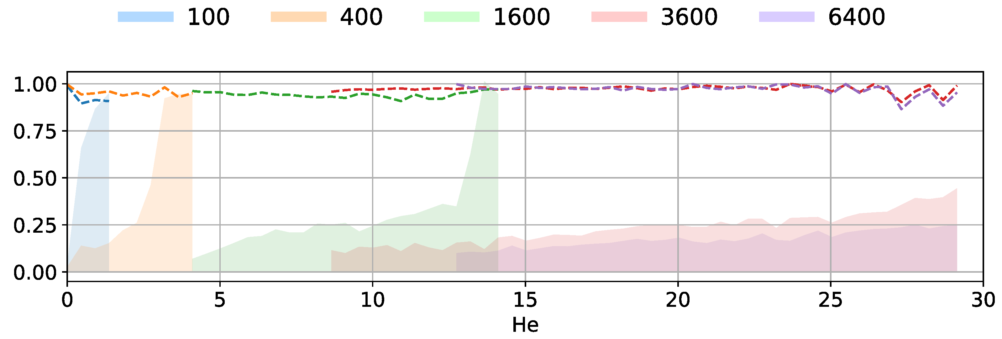
In Figure 4, the radiated sound power estimate compared to the ground truth is compared to the ERP estimation based on a generalized ${\chi }^2$ distribution. Several dashed lines and shaded areas are shown in the plot, describing the results of different the uniform resolution of a total of 100, 400, 1600, 3600, and 6400 points. Firstly, in blue, the relative accuracy ${\eta }_{{\chi }^2}$ of the (true) ERP (estimated by the reference solution data) and the ERP predicted by ${\chi }^2$ distribution descriptive statistics of the velocity data from the GPR

$${\eta }_{{\chi }^2}=1-|\frac{P_{\mathrm{a}},\mathrm{ERP}}{P_{\mathrm{a},\mathrm{ERP},{\chi }^2}}-1|=1-{ϵ}_{{\chi }^2}.$$

Secondly, the blue-shaded band visualizes the predictive uncertainty ${\sigma }_{\ast }^2$ of the GPR. The mean and variance of statistical ERP prediction methods are in good agreement with the Monte Carlo simulation ${\eta }_{MC}$ (mean deviations less than ${10}^{-5}$ for each study), suggesting that fast computations using descriptive statistics based on the ${\chi }^2$ distribution are a valuable and computationally efficient alternative.

It is noticeable that the quality of the GPR interpolation is strongly governed by the predictive uncertainty ${\sigma }_{\ast }^2$, which indicates how much can be described by the deterministic part of the GPR. In the case of a value of zero, the deterministic part can accurately describe the data. However, as the value increases towards 1, the descriptive capabilities of the GPR decrease, and one can see large deviations in the field plots compared to the ground truth. It means that the mean of the GPR is significantly different from the provided velocity data. In such a case, the modes of vibration cannot be explained by the GPR anymore. Figure 4 clearly shows that with an increasing number of training points, the limit where the variational GPR can still explain the surface vibration velocity rises monotonically. For a resolution of 100 points, vibration characteristics below a Helmholtz number of ${\mathrm{He}}_{\mathrm{crit}}=0.25$ can be resolved. For 400 points, this limit increases to a Helmholtz number of ${\mathrm{He}}_{\mathrm{crit}}=2.5$, for 1600 points to about a Helmholtz number of ${\mathrm{He}}_{\mathrm{crit}}=13$, for 3600 and 6400 points above the maximum Helmholtz number of interest ${\mathrm{He}}_{\mathrm{crit}}>29$. It is observed, that the predictive uncertainty is larger for 3600 in the whole frequency range compared to a 6400 points resolution.

Figure 4. Evolution of the relative accuracies ${\eta }_{{\chi }^2}$ (dashed line) and predictive uncertainties ${\sigma }_{\ast }^2$ (shaded area) of the corresponding GPR as a function of the Helmholtz number, for different uniform resolutions of a total of 100 (blue), 400 (orange), 1600 (green), 3600 (magenta), 6400 (violet) points. The SNR level is 1000/1.

Figure 4. Evolution of the relative accuracies ${\eta }_{{\chi }^2}$ (dashed line) and predictive uncertainties ${\sigma }_{\ast }^2$ (shaded area) of the corresponding GPR as a function of the Helmholtz number, for different uniform resolutions of a total of 100 (blue), 400 (orange), 1600 (green), 3600 (magenta), 6400 (violet) points. The SNR level is 1000/1.

5.3. Correlation Between Sound Power Error $ϵ$ and Predicted Uncertainty ${\sigma }_{\ast }^2$

In this section, we will investigate Hypothesis 3. According to Figure 4, there is no direct correlation between the interpolation error of the surface velocity and the predictive uncertainty ${\sigma }_{\ast }^2$ of the GPR visible. As soon as the GPR cannot explain the data by its deterministic part anymore, the predictive uncertainty ${\sigma }_{\ast }^2$ increases sharply, indicating that there are too few training points for the GPR. However, the error in the sound power (equal to the integrated surface velocity) increases only slightly.

Even at high GPR noise levels, the error of the predicted ERP is low. There is no clear trend whether the uniform or the Latin hypercube sampling performs better.

For a detailed analysis of the training time, the individual timings were separated into datasets, where the predictive uncertainty ${\sigma }_{\ast }^2$ is low and another where it is high. The separation was performed based on a critical Helmholtz number ${\mathrm{He}}_{\mathrm{crit}}$ as a selector; everything below was judged as low noise, and everything above was regarded as a high noise region. In the respective ranges, the mean over all GPRs is computed. The means of the training times for each investigated set of are reported in

Table 2. GPR mean training times $t_{\mathrm{tran}}$ of the individual GPRs of the real and imaginary part.

Run	${\overline{\mathit{t}}}_{\mathbf{tran},\mathbf{real}}$	${\overline{\mathit{t}}}_{\mathbf{tran},\mathbf{real}}$	${\overline{\mathit{t}}}_{\mathbf{tran},\mathbf{imag}}$	${\overline{\mathit{t}}}_{\mathbf{tran},\mathbf{imag}}$
	$>{\mathbf{He}}_{\mathbf{crit}}$	$<{\mathbf{He}}_{\mathbf{crit}}$	$>{\mathbf{He}}_{\mathbf{crit}}$	$<{\mathbf{He}}_{\mathbf{crit}}$
100, uni	2.626	0.428	2.589	0.256
400, uni	4.380	4.951	4.288	2.764
1600, uni	43.244	7.982	45.849	9.108
3600, uni	-	28.952	-	38.339
6400, uni	-	68.506	-	58.513

, with training iterations over 1500 epochs to reach the low noise levels (Apple M4 Chip 10 Cores, 32 GB RAM, Apple Inc., Cupertino, CA, USA). The means are computed over all GPRs fulfilling the condition of the critical Helmholtz number ${\mathrm{He}}_{\mathrm{crit}}$. For a high number of training points and as soon as the GPR noise level increases, the training time increases substantially. There was no significant difference between the Latin hypercube sampling and the uniform sampling.

5.4. Uniform Sampling Versus Latin-Hypercube Sampling for the Surface Velocity

This section discusses two types of common (automated) data sampling strategies in connection with the underlying process specification (Hypothesis 4). The sampling strategies are as follows: first, a regular fit onto the geometry for uniform plate-like domains; second, a commonly used sampling strategy for arbitrary sampling spaces. The first strategy of uniform sampling is ideal in the case of uniform plate stiffness and the coordinate-sampling-aligned mode shapes. However, the results might deteriorate for inhomogeneous material, inhomogeneous plate thickness, non-rectangular geometries, non-uniform clamping at the boundaries, and other effects that produce modes with localized gradients and non-alignment with the sampling strategy. Therefore, we look into the details of the surface velocity predictions based on the two sampling strategies (using an exact GPR, which works for a low number of training points).

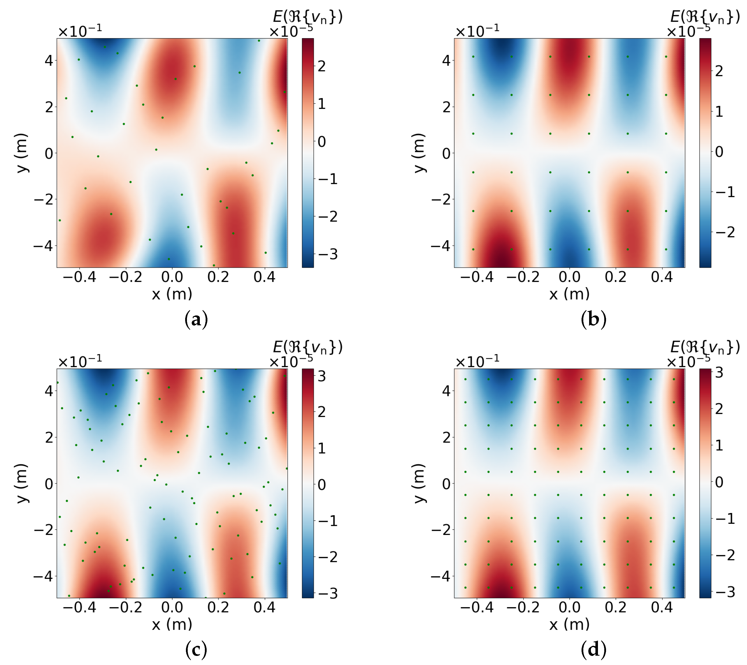
Figure 5 depicts the expected value and Figure 6 the standard deviation of the real part of the normal velocity for the respective sampling strategies for a frequency of 313 Hz.

The expected value is in close range to the ground truth of the reference data for both sampling strategies. For the standard deviations, uniform sampling leads to a significantly lower overall standard deviation between the sampling points compared to Latin hypercube sampling. For the Latin hypercube sampling, some blind spots on the geometry arise, where no support points of the GP are present, leading to a larger standard deviation in the prediction. These increased standard deviation spots could be used for adaptive refinement; however, they typically are located on the boundaries of the domain. This naive approach can be improved by using the variance-based refinement strategy presented in [48]. Another possibility is a modified version of the expected improvement [49].

5.5. Design of Experiement Using Adaptive Refinement

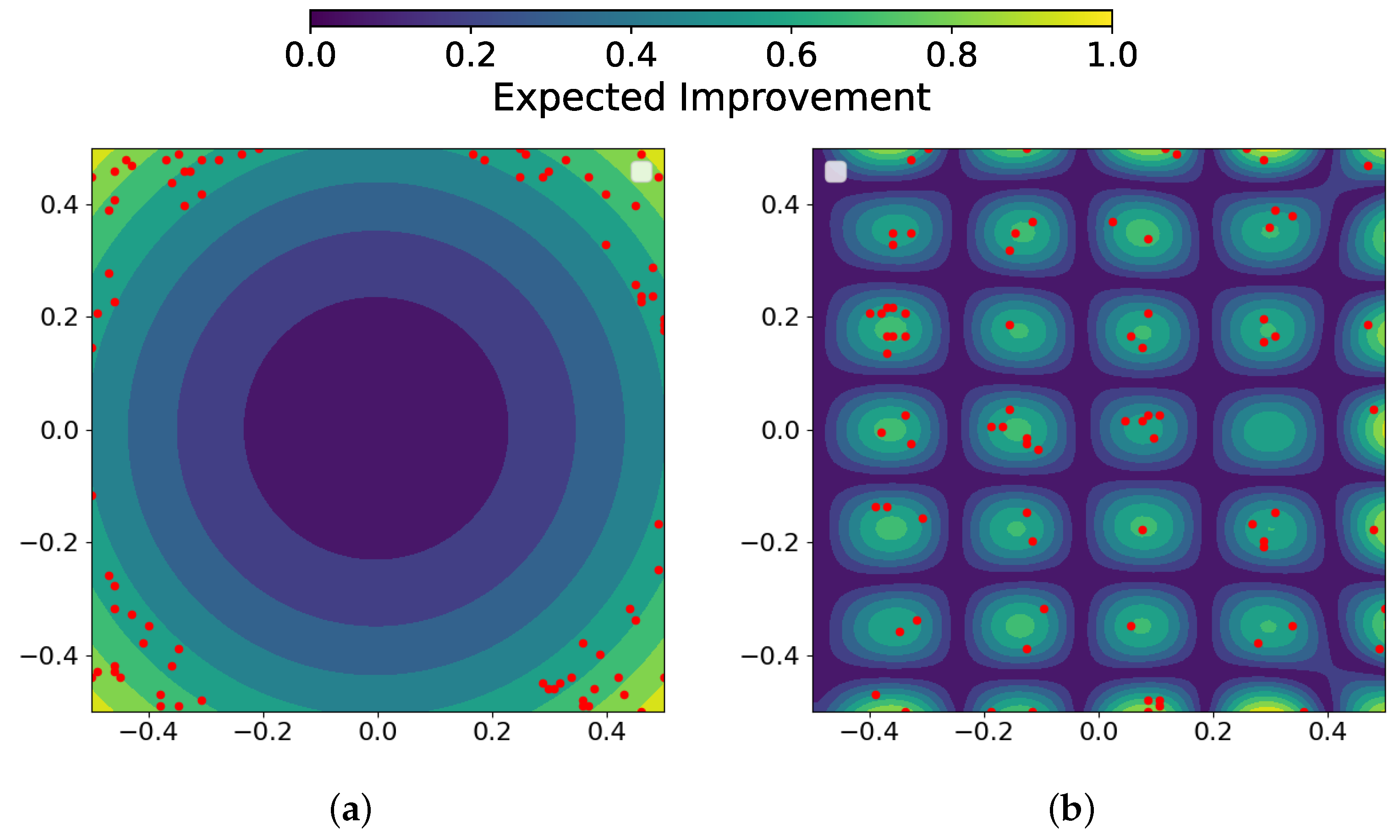
To test Hypothesis 5, an adaptive refinement procedure as described in Section 2.5 was performed. As a stopping criterion, the normalized noise of the GPR exceeds was used with a threshold of 0.01. Figure 7 shows the frequency of 1250 Hz, the $EI\left(x\right)$ at the start of the adaptive refinement iterations, and at the third stage of the adaptive refinement iterations for the real part of the surface normal velocity field. At the first stage (Figure 7a), the GP is not able to resolve the velocity field adequately, and the EI suggests adding points at the domain corners. This is expected as at this stage the field is mostly described by noise everywhere. Due to the intended randomness in the point selection, the procedure remains robust and at the third stage (Figure 7b).

Figure 8 shows the effects of the adaptive refinement procedure on the sound power error and GPR predictive uncertainty as a function of the Helmholtz number. At the initial stage, before the refinement, 400 uniform training points were considered. As a comparison, this setup without adaptive refinement predicted a low noise in the function output until a Helmholtz number of about 2.5 (see Figure 4). In comparison, with the adaptive refinement procedure, a robust prediction was possible up to a Helmholtz number of 11. This accuracy is comparable to that of predictions provided by 1600 uniform training points, despite using only 1200 data points. It is observed that during the adaptive refinement, the predictive uncertainty is lower in the converged region (He < 11) compared to the predictions using 1600 uniform training points. However, the ERP estimate is slightly less accurate compared to the estimations based on 1600 uniform training points due to the early stopping criterion selected. The estimates were robust regarding the initial training distribution; when using a Latin hypercube sampling initially, comparable results were obtained.

5.6. Detailed Comparison of Sound Power Estimates

In Figure 9, the sound power estimate based on the ERP is compared to the one using BEM (Hypothesis 6). For the current case, below the coincidence frequency ${\mathrm{He}}_{\mathrm{co}}$ (red line in Figure 9), the ERP estimate is not an accurate measure for the radiated sound power. Typically, with increasing frequency, the radiation efficiency increases, and as soon as it turns to one, the ERP and the BEM estimate coincide. Under this condition, the ERP measure is preferable, as the statistical estimation presented in this article enables the statistical description and estimates to be carried out. Regarding the simulation time, at low frequencies, a relatively coarse training point distribution is sufficient, allowing for the computation of the Monte Carlo simulation within a reasonable time frame. As indicated by the results in Figure 4, the statistical values estimated by 100 simulations are sufficiently close to the analytically derived ones.

5.7. Computational Performance Using Pre-Trained Models

Finally, we tested if a significant speedup of the training time is possible using a pre-trained model (Hypothesis 7). Typically, during production, each product will not deviate much from the previous one (as long as it is of high quality); therefore, it might be interesting to use a pre-trained model.

Table 3. GPR mean training times below the critical Helmholtz number $\mathrm{He}<{\mathrm{He}}_{\mathrm{crit}}$. The abbreviation uni stands for uniform sampling.

Run	$\mathit{E}\left[{\mathit{t}}_{\mathbf{tran}}\right]$	$\sqrt{\mathit{VAR}\left[{\mathit{t}}_{\mathbf{tran}}\right]}$	Training Epochs	Pre-Trained Model Used
1600, uni	5.57	1.94	1500	no
1600, uni	3.59	0.91	1500	yes
1600, uni	2.23	0.09	150	yes
1600, uni	1.14	0.12	75	yes

compares the training times for several configurations. When using 1600 training points with the GPR setup, 1500 epochs of training, and a batch size of 1024, it took on average 5.57 s to train from scratch (in the region where convergence is achieved). When using a pre-trained GPR, the training time was reduced to 3.6 s (a nearly 36% reduction from 5.57 s to 3.6 s) with a standard deviation of 0.91 s. By relaxing the number of epochs (while still obtaining a converged GPR), the training time was reduced by approximately 68% from 3.6 s to 1.14 s. Overall, the mean training time was reduced from 5.57 s to 1.14 s, which yields an increase in computational performance of 79%.

5.8. Influence of Measurement Noise

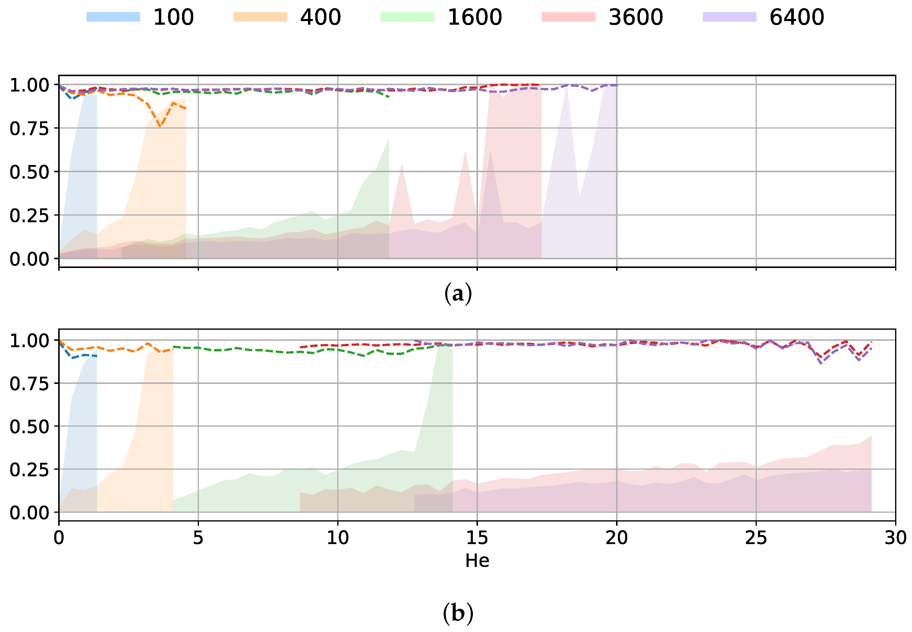
All previous investigations were based on a laser vibrometry measurement with a signal-to-noise ratio (SNR) of 1000/1, which represents a level of measurement quality that can be achieved for many applications. To test the effect of increased measurement noise on the proposed workflow (Hypothesis 8), the noise factor introduced in Section 3 was increased to $k_{\mathrm{noise}}=0.1$, representing a signal-to-noise ratio (SNR) of 10/1. Figure 10 depicts the evolution of the relative accuracy ${\eta }_{{\chi }^2}$ and the predictive uncertainty ${\sigma }_{\ast }^2$ as a function of the Helmholtz number for the increased noise level. One can observe that the method remains robust despite the increased measurement noise, and the GPR can interpolate the normal velocity field accurately for an adequate number of samples. Especially at a high number of samples, the results show a decreased critical Helmholtz number. Consequently, more samples are required to describe noisy measurement data in contrast to data with low SNR.

6. Conclusions

Initially, we identify four specifications for a measurement system for acoustic end-of-line testing to meet vibroacoustic requirements. Specification 1, to perform measurements at different locations, both contactless and without any additional assembly cost, was realized by a Laser scanning vibrometer setup. Specification 2 of the measurement system, which measures the accuracy and uncertainty of data prediction using a self-learned data-driven method, was achieved by the demonstration of the adaptive refinement method in combination with the underlying GPR. Specification 3, that the technique should provide data that give the maximum valuable insight into specific characteristics where deviations occurred over time, was not within the scope of the current investigation; however, it can be inferred through a comparative evaluation using the pre-trained models. The fourth specification that measurement and processing times should fit into the production cycle of a production line was demonstrated by the investigated hypotheses. The outcome of Hypothesis 1 is that the algorithm derived provides real-time capability regarding the sampling cycle of the laser scanning vibrometry system with fixed sample averaging and fixed measurement uncertainty thresholds. We demonstrated that the number of training points for Gaussian process regression positively correlates with the upper frequency limit at which the deterministic part of the Gaussian process can accurately model the surface normal velocity and sound prediction. We found that the ERP error with respect to the ground truth does not correlate with the noise in the velocity prediction from the GPR for the benchmark problem used. We found that Latin hypercube sampling, with the same number of sampling points, does not show better performance in training compared to uniform sampling. We also demonstrated the limitations of the ERP-based estimates by comparing them to sound power predictions using BEM. At higher oscillation frequencies, the ERP predicted sound power delivers accurate results. The computational performance was significantly increased (79% less time consumed) using transfer learning, based on pre-trained models. Overall, the use of GPyTorch over scikit-learn reduced the processing time by a factor of 60. Furthermore, we investigated the influence of uncorrelated noise on the measurement data, where we observed an increased number of measurement points to describe noisy measurement data.

Finally, we want to point out perspectives to improve the GPR modeling, including a spatially varying measurement noise distribution and improvement of the adaptive refinement strategy. The measurement uncertainty based on the local measurement point of the experimental setup can be modeled within the GPR and, therefore, considered by the sound prediction method. A direct extension to measurement noise distribution in space (variation in input locations) can be undertaken via Variational Heteroscedastic Gaussian process regression [50]. Another direction would be to develop an improved adaptive refinement strategy that eliminates oscillatory behavior as soon as the predictive uncertainty increases. Ghosh et al. [51] propose a framework that partitions prediction uncertainty based on fidelity levels, allowing for a more nuanced approach to experimental design that considers both the cost and the expected information gain from various data sources. This strategy not only enhances the efficiency of the design process but also provides a systematic method for integrating information from different fidelity levels, thereby enriching the overall understanding of the system under investigation.

References

1. Kumar, S.; Forster, H.M.; Bailey, P.; Griffiths, T.D. Mapping Unpleasantness of Sounds to Their Auditory Representation. J. Acoust. Soc. Am. 2008, 124, 3810–3817. [Google Scholar] [CrossRef]
2. Marburg, S. Boundary Element Method for Time-Harmonic Acoustic Problems. In Computational Acoustics; Kaltenbacher, M., Ed.; CISM International Centre for Mechanical Sciences; Springer International Publishing: Cham, Switzerland, 2018; pp. 69–158. [Google Scholar] [CrossRef]
3. Vachálek, J.; Bartalskỳ, L.; Rovnỳ, O.; Šišmišová, D.; Morháč, M.; Lokšík, M. The digital twin of an industrial production line within the industry 4.0 concept. In Proceedings of the 2017 21st International Conference on Process Control (PC), Štrbské Pleso, Slovakia, 6–9 June 2017; pp. 258–262. [Google Scholar]
4. Klippel, W. End-of-line testing. In Assembly Line-Theory and Practice; Grzechca, W., Ed.; Books on Demand: Norderstedt, Germany, 2011; pp. 181–206. [Google Scholar]
5. Wurzinger, A.; Kraxberger, F.; Maurerlehner, P.; Mayr-Mittermüller, B.; Rucz, P.; Sima, H.; Kaltenbacher, M.; Schoder, S. Experimental Prediction Method of Free-Field Sound Emissions Using the Boundary Element Method and Laser Scanning Vibrometry. Acoustics 2024, 6, 65–82. [Google Scholar] [CrossRef]
6. Rasmussen, C.E. Gaussian processes in machine learning. In Summer School on Machine Learning; Springer: Berlin/Heidelberg, Germany, 2003; pp. 63–71. [Google Scholar]
7. Wurzinger, A.; Kraxberger, F.; Mayr-Mittermüller, B.; Rucz, P.; Sima, H.; Kaltenbacher, M.; Schoder, S. Assessment of vibro-acoustic sound emissions based on structural dynamics. In Proceedings of the Proceedings of DAGA 2024, Hannover, Germany, 18–21 March 2024. [Google Scholar]
8. Li, J.; Wang, H. Gaussian Processes Regression for Uncertainty Quantification: An Introductory Tutorial. arXiv 2025, arXiv:2502.03090. [Google Scholar] [CrossRef]
9. Schulz, E.; Speekenbrink, M.; Krause, A. A Tutorial on Gaussian Process Regression: Modelling, Exploring, and Exploiting Functions. J. Math. Psychol. 2018, 85, 1–16. [Google Scholar] [CrossRef]
10. Tuo, R.; Wang, W. Uncertainty quantification for Bayesian optimization. In Proceedings of the International Conference on Artificial Intelligence and Statistics, Virtual, 28–30 March 2022; pp. 2862–2884. [Google Scholar]
11. Bect, J.; Bachoc, F.; Ginsbourger, D. A Supermartingale Approach to Gaussian Process Based Sequential Design of Experiments. Bernoulli 2019, 25, 2883–2919. [Google Scholar] [CrossRef]
12. Jault, D.; Gillet, N.; Schaeffer, N.; Mandéa, M. Local Estimation of Quasi-Geostrophic Flows in Earth’s Core. Geophys. J. Int. 2023, 234, 494–511. [Google Scholar] [CrossRef]
13. Xia, G.; Han, Z.; Zhao, B.; Wang, X. Unmanned Surface Vehicle Collision Avoidance Trajectory Planning in an Uncertain Environment. IEEE Access 2020, 8, 207844–207857. [Google Scholar] [CrossRef]
14. Kocev, B.; Hahn, H.K.; Linsen, L.; Wells, W.M.; Kikinis, R. Uncertainty-Aware Asynchronous Scattered Motion Interpolation Using Gaussian Process Regression. Comput. Med. Imaging Graph. 2019, 72, 1–12. [Google Scholar] [CrossRef]
15. Jahanandish, M.H.; Fey, N.P.; Hoyt, K. Lower Limb Motion Estimation Using Ultrasound Imaging: A Framework for Assistive Device Control. IEEE J. Biomed. Health Inform. 2019, 23, 2505–2514. [Google Scholar] [CrossRef]
16. Omainska, M. Visual Pursuit With Switched Motion Estimation and Rigid Body Gaussian Processes. Trans. Inst. Syst. Control Inf. Eng. 2023, 36, 327–335. [Google Scholar] [CrossRef]
17. Binois, M.; Huang, J.; Gramacy, R.B.; Ludkovski, M. Replication or Exploration? Sequential Design for Stochastic Simulation Experiments. Technometrics 2018, 61, 7–23. [Google Scholar] [CrossRef]
18. Gardner, J.; Pleiss, G.; Weinberger, K.Q.; Bindel, D.; Wilson, A.G. Gpytorch: Blackbox matrix-matrix gaussian process inference with gpu acceleration. Adv. Neural Inf. Process. Syst. 2018, 31. [Google Scholar]
19. Raychaudhuri, S. Introduction to monte carlo simulation. In Proceedings of the 2008 Winter Simulation Conference, Miami, FL, USA, 7–10 December 2008; pp. 91–100. [Google Scholar]
20. Wurzinger, A.; Heidegger, P.; Kraxberger, F.; Mayr-Mittermüller, B.; Sima, H.; Kaltenbacher, M.; Schoder, S. Prediction of vibro-acoustic sound emissions based on mapped structural dynamics. In Proceedings of the INTER-NOISE and NOISE-CON Congress and Conference Proceedings, Nantes, France, 25–29 August 2024; Volume 270, pp. 8251–8260. [Google Scholar] [CrossRef]
21. Pedregosa, F.; Varoquaux, G.; Gramfort, A.; Michel, V.; Thirion, B.; Grisel, O.; Blondel, M.; Prettenhofer, P.; Weiss, R.; Dubourg, V.; et al. Scikit-Learn: Machine Learning in Python. J. Mach. Learn. Res. 2011, 12, 2825–2830. [Google Scholar]
22. Bilionis, I.; Zabaras, N. Multi-Output Local Gaussian Process Regression: Applications to Uncertainty Quantification. J. Comput. Phys. 2012, 231, 5718–5746. [Google Scholar] [CrossRef]
23. Mones, L.; Bernstein, N.; Csányi, G. Exploration, Sampling, And Reconstruction of Free Energy Surfaces with Gaussian Process Regression. J. Chem. Theory Comput. 2016, 12, 5100–5110. [Google Scholar] [CrossRef]
24. Titsias, M. Variational learning of inducing variables in sparse Gaussian processes. In Proceedings of the Artificial Intelligence and Statistics, Clearwater Beach, FL, USA, 16–18 April 2009; pp. 567–574. [Google Scholar]
25. Maddox, W.J.; Stanton, S.; Wilson, A.G. Conditioning Sparse Variational Gaussian Processes for Online Decision-making. In Proceedings of the Advances in Neural Information Processing Systems; Ranzato, M., Beygelzimer, A., Dauphin, Y., Liang, P., Vaughan, J.W., Eds.; Curran Associates, Inc.: New York, NY, USA, 2021; Volume 34, pp. 6365–6379. [Google Scholar]
26. Bauer, M.; Van der Wilk, M.; Rasmussen, C.E. Understanding probabilistic sparse Gaussian process approximations. Adv. Neural Inf. Process. Syst. 2016, 29. [Google Scholar]
27. Williams, C.; Rasmussen, C. Gaussian processes for regression. Adv. Neural Inf. Process. Syst. 1995, 8. [Google Scholar]
28. Rasmussen, C.E.; Williams, C.K.I. Gaussian Processes for Machine Learning, 3rd ed.; Adaptive Computation and Machine Learning; MIT Press: Cambridge, MA, USA, 2008. [Google Scholar]
29. Fiala, P.; Rucz, P. NiHu: An Open Source C++ BEM Library. Adv. Eng. Softw. 2014, 75, 101–112. [Google Scholar] [CrossRef]
30. Burton, A.J.; Miller, G.F. The Application of Integral Equation Methods to the Numerical Solution of Some Exterior Boundary-Value Problems. Proc. R. Soc. Lond. 1971, 323, 201–210. [Google Scholar] [CrossRef]
31. Luegmair, M.; Münch, H. Advanced Equivalent Radiated Power (ERP) Calculation for Early Vibro-acoustic Product Optimization. In Proceedings of the The 22nd International Congress on Sound and Vibration, Florence, Italy, 12–16 July 2015. [Google Scholar]
32. Fritze, D.; Marburg, S.; Hardtke, H.J. Estimation of radiated sound power: A case study on common approximation methods. Acta Acust. United Acust. 2009, 95, 833–842. [Google Scholar] [CrossRef]
33. Cremer, L.; Heckl, M.; Petersson, B. Sound Radiation from Structures. In Structure-Borne Sound: Structural Vibrations and Sound Radiation at Audio Frequencies; Springer: Berlin/Heidelberg, Germany, 2005; pp. 449–535. [Google Scholar] [CrossRef]
34. Kvist, K.; Sorokin, S.V.; Larsen, J.B. Radiation Efficiency Varying Equivalent Radiated Power. J. Acoust. Soc. Am. 2025, 157, 169–177. [Google Scholar] [CrossRef] [PubMed]
35. Das, A.; Geisler, W.S. Methods to integrate multinormals and compute classification measures. arXiv 2020, arXiv:2012.14331. [Google Scholar]
36. Schoder, S.; Roppert, K. openCFS: Open Source Finite Element Software for Coupled Field Simulation—Part Acoustics. arXiv 2022, arXiv:2207.04443. [Google Scholar] [CrossRef]
37. Langer, P.; Maeder, M.; Guist, C.; Krause, M.; Marburg, S. More Than Six Elements Per Wavelength: The Practical Use of Structural Finite Element Models and Their Accuracy in Comparison with Experimental Results. J. Comput. Acoust. 2017, 25, 1750025. [Google Scholar] [CrossRef]
38. Schoder, S.; Roppert, K.; Weitz, M.; Junger, C.; Kaltenbacher, M. Aeroacoustic source term computation based on radial basis functions. Int. J. Numer. Methods Eng. 2020, 121, 2051–2067. [Google Scholar] [CrossRef]
39. Hensman, J.; Matthews, A.; Ghahramani, Z. Scalable Variational Gaussian Process Classification. arXiv 2014, arXiv:1411.2005. [Google Scholar] [CrossRef]
40. Blei, D.M.; Kucukelbir, A.; McAuliffe, J.D. Variational Inference: A Review for Statisticians. J. Am. Stat. Assoc. 2017, 112, 859–877. [Google Scholar] [CrossRef]
41. Kullback, S.; Leibler, R.A. On information and sufficiency. Ann. Math. Stat. 1951, 22, 79–86. [Google Scholar] [CrossRef]
42. Snelson, E.; Ghahramani, Z. Sparse Gaussian processes using pseudo-inputs. Adv. Neural Inf. Process. Syst. 2005, 18. [Google Scholar]
43. Hensman, J.; Fusi, N.; Lawrence, N.D. Gaussian Processes for Big Data. arXiv 2013, arXiv:1309.6835. [Google Scholar] [CrossRef]
44. Dai, Z.; Damianou, A.; Hensman, J.; Lawrence, N. Gaussian Process Models with Parallelization and GPU acceleration. arXiv 2014, arXiv:1410.4984. [Google Scholar] [CrossRef]
45. Gal, Y.; van der Wilk, M.; Rasmussen, C.E. Distributed Variational Inference in Sparse Gaussian Process Regression and Latent Variable Models. In Proceedings of the Advances in Neural Information Processing Systems; Ghahramani, Z., Welling, M., Cortes, C., Lawrence, N., Weinberger, K., Eds.; Curran Associates, Inc.: New York, NY, USA, 2014; Volume 27. [Google Scholar]
46. Paszke, A.; Gross, S.; Massa, F.; Lerer, A.; Bradbury, J.; Chanan, G.; Killeen, T.; Lin, Z.; Gimelshein, N.; Antiga, L.; et al. PyTorch: An Imperative Style, High-Performance Deep Learning Library. In Advances in Neural Information Processing Systems 32; Curran Associates, Inc.: New York, NY, USA, 2019; pp. 8024–8035. [Google Scholar]
47. Kingma, D.P.; Ba, J. Adam: A method for stochastic optimization. arXiv 2014, arXiv:1412.6980. [Google Scholar]
48. Krause, A.; Singh, A.; Guestrin, C. Near-optimal sensor placements in Gaussian processes: Theory, efficient algorithms and empirical studies. J. Mach. Learn. Res. 2008, 9, 235–284. [Google Scholar]
49. Jones, D.R.; Schonlau, M.; Welch, W.J. Efficient global optimization of expensive black-box functions. J. Glob. Optim. 1998, 13, 455–492. [Google Scholar] [CrossRef]
50. Lázaro-Gredilla, M.; Titsias, M.K. Variational Heteroscedastic Gaussian Process Regression. In Proceedings of the ICML, Washington, DC, USA, 28 June–2 July 2011; pp. 841–848. [Google Scholar]
51. Ghosh, S.; Kristensen, J.; Zhang, Y.; Subber, W.; Wang, L. A Strategy for Adaptive Sampling of Multi-Fidelity Gaussian Processes to Reduce Predictive Uncertainty; American Society of Mechanical Engineers: New York, NY, USA, 2019. [Google Scholar] [CrossRef]
Figure 1. Schematic of the presented workflow predicting the radiated sound field based on surface velocity measurements, including an adaptive refinement procedure.
Applsci 15 10652 g001
Figure 2. Top view of the investigated plate with an exemplary set of 36 (red) and 100 (blue) measurement points, based on Latin hypercube (b) and uniform (c) sampling, respectively. (a) Simulation setup, with force F z and boundary conditions [5]. (b) Latin hypercube sampling. (c) Uniform sampling.
Applsci 15 10652 g002
Figure 3. Solution of the benchmark problem. Indicated eigenmodes at He = 0.024, 0.06, 0.22, 0.38, 0.43, 0.98, 1.43, 1.85. The coincidence frequency for this setup is He = 3.6 . (a) Real part of the mode shape for selected structural eigenmodes. (b) Radiated sound power based on BEM ( P a ) and ERP.
Applsci 15 10652 g003
Figure 5. Mean of the real value of the normal velocity v n at f = 313 Hz , Latin hypercube sampling, and uniform sampling for n = 36 and n = 100 pseudo measurement points indicated in green. (a) Latin hypercube sampling with n = 36 . (b) Uniform sampling with n = 36 . (c) Latin hypercube sampling with n = 100 . (d) Uniform sampling with n = 100 .
Applsci 15 10652 g005
Figure 6. Standard deviation of the real value of the normal velocity v n at f = 313 Hz , latin hypercube and uniform sampling for n = 36 and n = 100 pseudo measurement points indicated in green. (a) Latin hypercube sampling with n = 36 . (b) Uniform sampling with n = 36 . (c) Latin hypercube sampling with n = 100 . (d) Uniform sampling with n = 100 .
Applsci 15 10652 g006
Figure 7. Two snapshots of E I ( x ) during the adaptive refinement procedure for the real part of the surface normal velocity. The red dots indicate the added training pairs to the GPR training for both the real and imaginary parts. (a) First stage. (b) Third stage.
Applsci 15 10652 g007
Figure 8. Evolution of the relative accuracy η χ 2 and the predictive uncertainty σ 2 as a function of the Helmholtz number. An initially uniform resolution of 400 was used, with random adaptive refinement. At the final stage, 1200 training points were considered.
Applsci 15 10652 g008
Figure 9. Comparison of the radiation efficiency, the relative ERP accuracy η χ 2 , and the predictive uncertainty σ 2 as a function of the Helmholtz number for the adaptive refinement case in Figure 8.
Applsci 15 10652 g009
Figure 10. Evolution of the relative accuracy η χ 2 and the predictive uncertainty σ 2 as a function of the Helmholtz number with an increased SNR. (a) Increased SNR: k noise = 0.1 . (b) Reference SNR: k noise = 0.001 .
Applsci 15 10652 g010