Authenticity at Risk: Key Factors in the Generation and Detection of Audio Deepfakes ^†

Abstract

Detecting audio deepfakes is crucial to ensure authenticity and security, especially in contexts where audio veracity can have critical implications, such as in the legal, security or human rights domains. Various elements, such as complex acoustic backgrounds, enhance the realism of deepfakes; however, their effect on the processes of creation and detection of deepfakes remains under-explored. This study systematically analyses how factors such as the acoustic environment, user type and signal-to-noise ratio influence the quality and detectability of deepfakes. For this study, we use the WELIVE dataset, which contains audio recordings of 14 female victims of gender-based violence in real and uncontrolled environments. The results indicate that the complexity of the acoustic scene affects both the generation and detection of deepfakes: classifiers, particularly the linear SVM, are more effective in complex acoustic environments, suggesting that simpler acoustic environments may facilitate the generation of more realistic deepfakes and, in turn, make it more difficult for classifiers to detect them. These findings underscore the need to develop adaptive models capable of handling diverse acoustic environments, thus improving detection reliability in dynamic and real-world contexts.

1. Introduction

In recent years, advances in machine learning (ML) technologies have led to the development of deepfakes, a technique that uses generative neural networks to create highly realistic fake multimedia content [1]. Deepfakes can manipulate images as well as video and audio, generating content that can deceive even trained observers. When combined with the Internet of Things (IoT), a wealth of new opportunities in uncountable applications such as personalized healthcare, manufacturing, transportation, smart homes, agriculture, or public safety is expected to impact our daily lives [2].

However, this combination also known as AIoT (Artificial Internet of Things), amplifies the potential risks posed by generative artificial intelligence, and in particular, of deepfakes: a vast network of cyberphysical devices (intelligent household gadgets, wearable devices including pulse sensors, accelerometers, microphones, and every other form of sensor) can serve as both a breeding ground for creating highly realistic deepfakes and a platform for their dissemination.

Audio deepfakes (AD), in particular, represent a significant evolution in media manipulation technology. Synthetic voice generation, also known as voice cloning, imitation or spoofing, is conducted by using advanced algorithms that can imitate a person’s voice with great precision, replicating not only pitch and timbre but also speech patterns and intonation. This technology has found applications in a variety of areas, from the entertainment industry to customer service automation. However, it has also opened the door to new types of fraud and manipulation, such as the creation of fake recordings that can be used to impersonate or commit scams.

The risks associated with deepfakes are many and varied. In general, they can be used to spread disinformation, influence public opinion, and perpetrate financial fraud. Malicious actors could exploit AIoT devices to collect data for generating deepfake content, while the interconnectedness of the network could facilitate rapid and widespread distribution of these fabricated media. This convergence of technologies exacerbates the challenges of detecting and mitigating the harmful impacts of deepfakes on individuals, organizations, and society as a whole [3] but even more on vulnerable persons, such as gender-based violence victims. In the context of cyberbullying, deepfakes can be particularly harmful, as they allow the creation and dissemination of false and compromising content that can damage the reputation of victims. Women, in particular, are a vulnerable group to such attacks, where audio deepfakes can be used to generate false recordings of an intimate or incriminating nature, exacerbating harassment and perpetuating gender-based violence in the digital sphere. This manipulative capacity not only affects privacy and personal safety but can also have serious psychological and social consequences for victims.

On the other hand, the problem of detecting audio deepfakes or antispoofing can be regarded as the task of verifying the identity of a speaker, and therefore, belongs to the field of speaker recognition, a specific application of biometrics, i.e., the science of identifying individuals based on unique physical or behavioral characteristics [4]. Again, the new generative artificial intelligence technologies bring singularities and challenges to this task [5].

The motivation for this research lies in the development of systems capable of detecting risk situations where a victim could be impersonated. To this end, we have used recordings obtained through a system called bindi [6] designed to assess a woman’s affective state through a set of intelligent wearable devices powered by ML, which capture her biosignals, including speech. However, in this paper, we will not be concerned with the modules regarding the affective state determination but only with the plausibility of generating credible audio deepfakes using voices recorded in similar circumstances. Thus, the choice of this dataset is based on the fact that the aforementioned recordings were made in realistic environments, without any constraints, and under authentic acoustic and emotional conditions. This is relevant for investigating the factors that may influence both the generation and detection of deepfakes, thus allowing us to identify in which real contexts it is easier to be fooled by deepfakes.

The main contribution of this work is a structured analysis of the impact of acoustic environments on both the generation and detection of deepfakes, an aspect that has not been systematically explored so far. In particular, we have evaluated (1) the influence of the speakers, (2) the type of acoustic environment, (3) the signal-to-noise ratio of speech over the background environment and (4) the models chosen for the detection. A highlight of our analysis is that we employ a real-life dataset, which allows the conditions of the generated audio to resemble real-world situations. However, the fact that this dataset is totally unconstrained and only weakly labeled compounds the analysis of the aforementioned factors since first, both the type of environment and the signal-to-noise (SNR) ratio had to be empirically estimated and second, a high imbalance of the classes of environments and SNRs appears.

This paper is organized as follows. We review the existing literature on the generation and detection of deepfakes in Section 2. Section 3, describes our chosen dataset–WELIVE–, explaining in detail how these data were collected. Section 4 explains the methodology employed including how the different factors used to interpret the results were obtained followed by the experimental settings specifications in Section 5 including pre-processing data, as well as the systems employed for the generation and detection of deepfakes in the recorded audios. In the Section 6, the findings of the experiments are presented. Finally, in the Section 7 and Section 8, we discuss the implications of the results obtained and propose directions for future research to improve the detection of deepfakes when they are generated from real acoustic environments, in order to protect victims of gender-based violence from impersonation attacks.

2. Related Work

Methods for generating audio include Text-To-Speech (TTS) synthesis and voice conversion (impersonation), as well as non-ML-generated audio (replay attacks), which involve replaying a victim’s voice recordings. While TTS converts text to speech using linguistic rules [7], voice conversion modifies the voice signal to sound like another person [8]. Current voice cloning methods can learn speech features from very few samples, producing speech that is almost indistinguishable from the original.

In 2016 The Voice Conversion Challenge 2016 [9] was released to compare different voice conversion techniques using a common dataset. The task to be solved was to transform the voice identity of a source speaker into that of a target speaker while preserving the linguistic content. Both speech conversion systems and TTS have advanced to the present day with approaches such as Deep Voice 3 [10], Fastspeech 2 [11] or Cyclegan-vc2 [12]. Among them, StarGANvc-v2 [13], a non-parallel and many-to-many speech conversion method that uses a generative adversarial network (GAN), is trained with only 20 English speakers, and outperforms previous models by being able to perform cross-language conversions, not requiring text labels and using Parallel WaveGAN [14] as a vocoder. These advances have led to the creation of numerous deepfake datasets such as H-voice [15], FakeAVCeleb [16], or Half-truth Speech [17], a dataset that used a text-to-speech model to generate and replace various words in audio clips.

The risk arises when, as the technology for generating audio deepfakes becomes more complex and accessible, non-experts can easily create fake audio. While this technology can be used for legitimate purposes, it can also be misused for disinformation and fraud [18,19,20]. To mitigate this impact, recent research has explored techniques for detecting audio deepfakes, a task also addressed in challenges such as ADD challenge 2022 [21] which sought to differentiate between various types of audio deepfakes and in ADD challenge 2023 [22] that reached further than the previous binary classification of real/fake, to locate manipulated intervals in partially fake speech, as well as to identify the source that generated the fake audio.

For the detection of these deepfakes, different techniques have been tested such as models based on logistic regression [23], quadratic SVMs [24], Res2Net [25], convolutional recurrent neural networks [26], EfficientCNN [27] or Deep4SNet, a model designed by [28] that seeks to turn the problem of fake audio detection into a computer vision task, by transforming audio data into the corresponding histogram images.

Some recent studies highlighting the scarcity of research focused on general audio, which encompasses all types of auditory content, including ambient sounds or speech, among others. In the absence of specific approaches in this field, the FakeSound dataset was developed [29]. For its creation, an audio-text model [30] was initially used to identify key audio segments whose modification could have a considerable impact. These segments were then masked and regenerated using generation models such as AudioSR [31], integrating them back into the original audio. To generate this dataset, they used AudioCaps [32] where they generated subtitles for audios in the wild.

However, to our knowledge, the generation and detection of such audios in real uncontrolled environments that were weakly labeled, as in our dataset, had not been previously investigated further than our preliminary results in [1] that we further develop in this paper.

3. The WELIVE Dataset

In this paper, we have used WELIVE (“Women and Emotion in real LIfe affectiVE computing dataset”), a multimodal affective computing dataset designed to address Gender-Based Violence (GBV) in real-world scenarios [33].

WELIVE contains multimodal contextual information about the daily routines of 14 Gender-Based Violence Victims (GBVV), aged 25–59 [34]. These women wore the bindi system for 7–10 days [6], which included a pendant that recorded audio, and a bracelet that measured physiological signals that were sent to a smartphone via a Bluetooth^® link. Global Positioning System (GPS) was also available but due to its high battery consumption, it was only activated sparsely. Finally, all this information captured was transmitted to a secure and encrypted server [6,35].

In addition, a smartphone application was available to report their location and emotions felt at any time of the day. Using this application, users could also send audio notes to verbally explain the situations that had triggered their tagged emotions. These audio notes were the data that we employed in this paper to generate the deepfakes. This application was included for the purpose of providing labels for the fine-tuning and adaptation of the models during a personalization stage and also provided a means of obtaining weak labels to train the ML models.

Before participating, the volunteers were interviewed by a psychologist specialized in GBV and completed a questionnaire to document their daily routines [33,36] (as well as a standardized test to assess their mental health status and specifically if they suffered from post-traumatic stress disorder). All the procedures were approved by the ethics and data protection committee of University Carlos III Madrid. Overall, WELIVE aims to investigate the impact of real-world environments on emotions and how these emotional states are reflected in vocal expressions and physiological responses [36]. Analyzing the impact of these real environments on the creation and detection of deepfakes can be essential for legal interventions aimed at enhancing the safety of GBVV.

4. Methodology

Since our aim was to quantify the influencing factors in the generation and detection of deepfakes in real-life situations, we characterized each audio note of WELIVE automatically with an estimated acoustic environment categorical label and an estimated Signal-to-Noise Ratio (SNR). The information about the user it belonged to is already available. Note that, since WELIVE is totally unconstrained, there is no balance of environments, speakers, or SNRs. In the following paragraphs, we explain the methods employed. A block diagram of the process followed to generate and detect audio deepfakes is provided in Figure 1 and detailed in Section 4.1 and Section 4.2. On the other hand, the process followed to obtain the influential factors in the generation and detection of audio deepfakes is outlined in Figure 2 and detailed in Section 4.3 and Section 4.4.

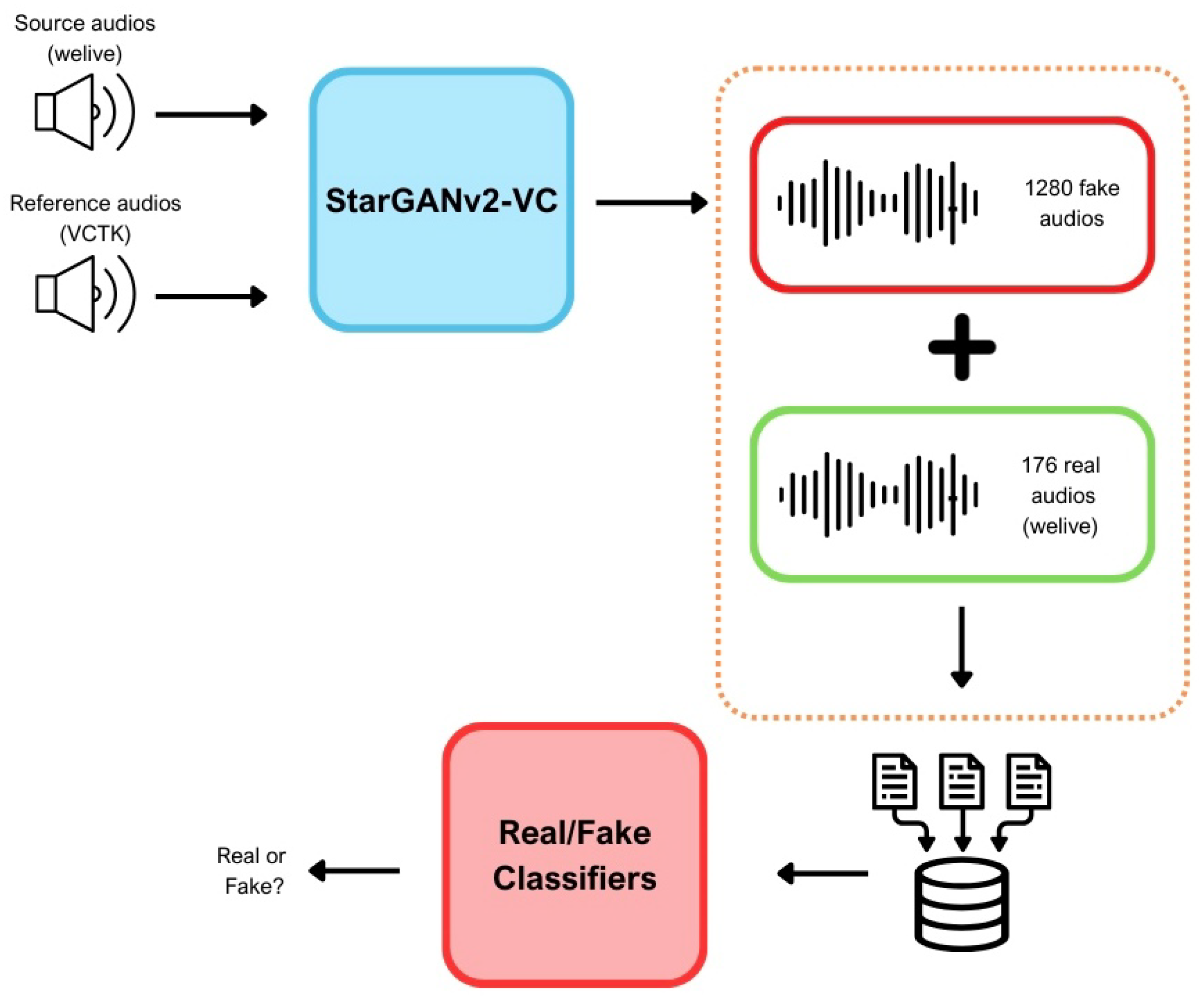
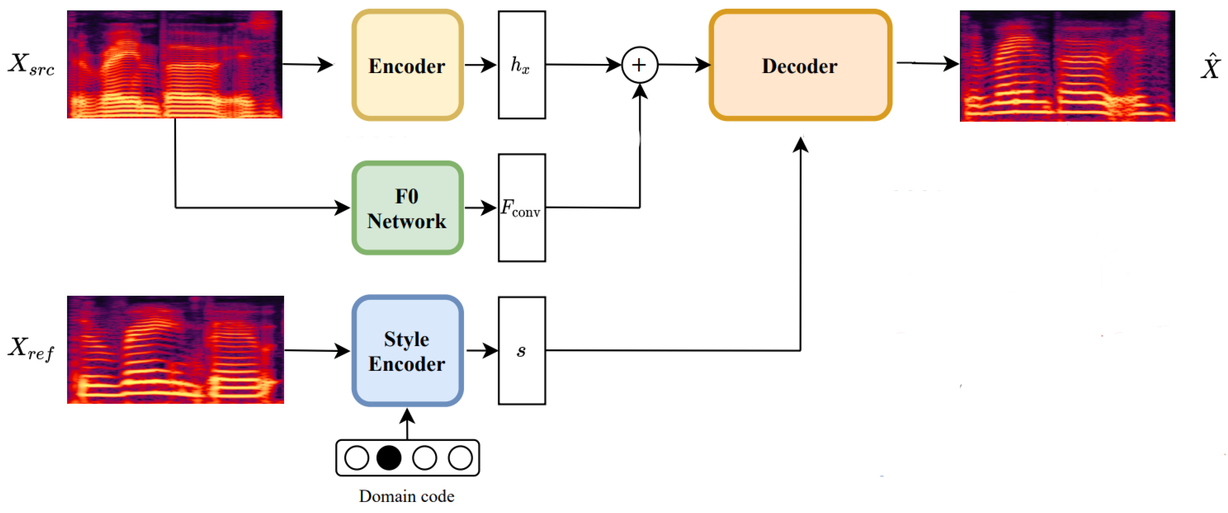
4.1. Generation of Deepfakes

In our study, audio sample generation was performed using the StarGANv2-VC [13], an unsupervised speech conversion (VC) model based on Generative Adversarial Networks (GANs), designed to perform speech conversions between multiple speakers without requiring parallel pairs of samples. One of its most outstanding features is its ability to transform the speech identity of one speaker into that of another while keeping the linguistic content intact. Despite being trained only on a limited dataset of 20 English speakers, the model is able to generalize to a variety of speech conversion tasks, such as one-to-many conversion, cross-lingual conversion, and voice style modification, such as falsetto or emotional voices.

The main components used for model inference are shown in Figure 3 adapted from [13]. To generate deepfakes, we have used the provided Python 3.12.3 inference notebook. The model is available for training at https://github.com/yl4579/StarGANv2-VC/tree/main (accesed on 6 November 2024).

• Generator (G): an encoder–decoder architecture that receives a mel-spectrogram as input and transforms it into one that reflects the vocal style and fundamental frequency (F0) of the target speaker. The style is obtained through a style encoder, while the fundamental frequency (F0) is derived through a network specialized in its detection.
• Style encoder (S) and mapping network (M): The style encoder extracts the stylistic features from a reference spectrogram, allowing conversion between different vocal styles.
• F0 extraction network: In order to preserve tonal consistency in the converted voice, the model uses a pre-trained F0 detection (JDC) network [37], which extracts the fundamental frequency, important to avoid distortions in the generated voice and ensures the pitch remains true to the target speaker.

An innovative feature of this model is the perceptual loss, which incorporates an automatic speech recognition (ASR) network and an F0 extraction system [37]. In addition, StarGANv2-VC is fully convolutional and, when integrated with an efficient vocoder such as Parallel WaveGAN [14], is capable of real-time speech conversions. The advantage of this system is that it achieves the conversion without the dependence on textual labels.

The source and reference audios to generate the deepfakes were extracted from WELIVE and VCTK [38] datasets, respectively, as will be detailed in Section 5.

4.2. Detection of Deepfakes

For deepfake detection, a Voice Activity Detection (VAD) method is employed to select the segments that contain speech. Then, the well-known Mel-Cepstral Frequency Coefficients (MFCC) [39] of the audios are extracted. The classifiers used include SVM [40] with a linear kernel, RF [41], KNN [42] and, Naive Bayes [43].

In this work, although most of our references employ deep learning techniques, these simple classifiers are chosen since the focus of this paper is to analyze the influential factors in both generation and detection in real-life situations and not to obtain the best classifier, despite the limited size of our dataset. Deep learning models, which rely on extracting complex patterns from large volumes of data, typically require a considerable number of samples to train effectively and generalize well to new inputs. Given that our dataset is small, these models could overfit, which would compromise their performance. Furthermore, simpler models already demonstrated satisfactory performance in our task, making the application of more advanced techniques unnecessary at this stage. Therefore, we leave the implementation of deep learning models for future work, for when we will have a larger dataset available.

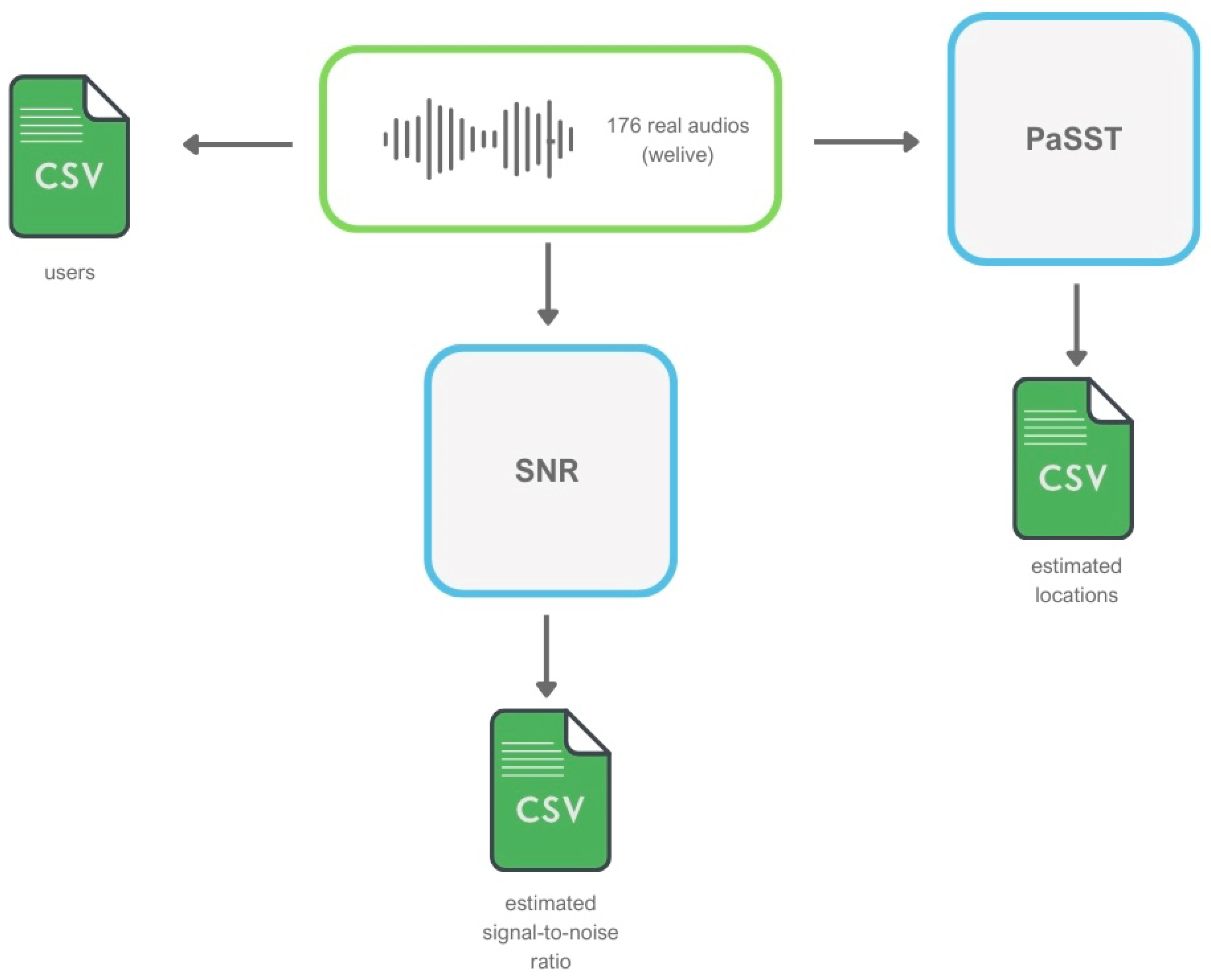
4.3. Automatic Determination of the Acoustic Context

To acoustically characterize the places where audio notes were recorded, we performed Acoustic Scene Classification (ASC). We used the PaSST (Patchout faSt Spectrogram Transformer) [44], a transformer-based model optimized for audio spectrogram processing, which addresses the limitations of traditional transformers in audio applications due to the quadratic growth in memory and computational requirements as the length of the input sequence increases. For this purpose, the authors introduced Patchout, a technique that significantly reduces the input sequence during training by randomly removing parts of it, which decreases both memory consumption and computational complexity. In addition, it introduces variants such as PaSST-U, where patches are removed in an unstructured manner, and PaSST-S, where entire rows or columns of patches are removed, based on approaches such as SpecAugment [45].

The PaSST architecture is depicted in Figure 4 and is extracted from [44], where the input spectrogram is first divided into small patches, to which positional encodings representing time and frequency are added. Then, a patch-out masking strategy is applied, and two special tokens are summed up to the resulting sequence: one for classification (C) and one for distillation (D). Subsequently, the sequence passes through several layers of self-attention and feed-forward networks (FFN), where the relationships between patches are processed. Finally, the processed tokens are combined and prediction is performed with a multi-layer perceptron (MLP).

PaSST has several applications in audio classification and labeling tasks, among which is the classification of acoustic scenes. In audio tagging in Audioset [46], it outperforms the AST transformer [47] and Convolutional Neural Networks (CNNs), improving the training speed and memory usage due to the patch-out process. In addition, it can be used in polyphonic musical instrument recognition.

We had previously trained the model for this task on a subset of WELIVE for which we had previous information about the location of the user. Note that there is no overlapping of these training audios with the audio notes mentioned before. The model was fine-tuned using five-fold stratified cross-validation, resulting in five models trained on different data partitions [36].

Then, the last layer of the PaSST Transformer was replaced by one with eight outputs and it was fine-tuned during 50 epochs using the stochastic gradient descend optimizer with a Nesterov momentum of $0.9$ and a learning rate of $0.0001$. Early-stopping was used on the F1-score macro, and the model performance reached the criteria at 30 epochs.

For each real-life audio note file, inference was performed using all five models. Predictions were considered valid if at least three of the models agreed on the classification. On the other hand, only seven audios were close to the decision boundary, i.e., for which at least three models did not agree with their prediction. These were listened to and re-labeled. The uncertainty was found to be due to audio files belonging to a category not accounted for in the labeling options, Street. Finally, audio notes were classified into nine different acoustic environments: Home, Work, Transport, Medical Center, Street, Bar, Restaurant, School and Cafeteria. More details about the training of this model are provided in [36].

4.4. Automatic Determination of the SNR

To calculate the SNR, the speech segments of the audio notes were selected as the ‘signal’ and the silent segment as ‘noise’. To separate these two signals, the PYANNOTE VAD [48] was used, which is able to accurately identify the parts where a speaker is active and those where she is not. Of the 176 audios analyzed, this system worked properly in 166 cases. In the remaining 10 audios, the VAD failed to locate speech, classifying all the time instances as silences. In this situation, we also tried to use PyPI’s VAD (https://github.com/MorenoLaQuatra/vad) (accessed on 1 August 2024), but the results were similar to those previously obtained, which led us to separate the speech signal manually in those particular cases. On the other hand, for the audios containing only speech, we used the immediately previously recorded audio signal as the associated noise signal since it had presumably been collected under similar conditions, thus ensuring consistency in the ambient noise conditions for the SNR calculation. Then, for the calculation of the SNR, we used the formula shown in the Equation (1), where $P_{\mathrm{signal}}$ represents the signal power and $P_{\mathrm{noise}}$ the noise power.

$$\mathrm{SNR}=10{\log }_{10}\left({\displaystyle \frac{P_{\mathrm{signal}}}{P_{\mathrm{noise}}}}\right)$$

(1)

Finally, the power of the signals was calculated following the Equation (2) where N is the total number of samples and $x_i$ is the value of the ith audio sample.

$$\mathrm{P}={\displaystyle \frac{1}{N}}\sum _{i=1}^N{x}_i^2$$

(2)

5. Experimental Settings

In this section, we detail the experimental procedures and settings used in the present study for the generation and detection of deepfakes. Our approach covers several key stages: data preparation, the process of generating synthetic audios using a speech conversion model, and the subsequent evaluation of deepfake detection using different classifiers. Additionally, in order to understand how different factors may influence the detection of deepfakes, we performed a comparison using two datasets: WELIVE, which contained both the deepfakes and real recordings captured in natural conditions without any constraints, and HABLA [49], a dataset with already synthesized fake audios.

5.1. Data Preprocessing

The audio notes from WELIVE were used as the source audios for deepfake generation, i.e., those for which the linguistic content would be preserved.

As detailed in Section 3, participants could record audio notes associated with emotion and location tags using the smartphone application. The audio notes were captured by the pendant, encoded using the OPUS codec [6], and transmitted to the mobile phone via Bluetooth^®. Then, the compressed data were sent to the server.

To conduct this research, we decoded the audio notes, which resulted in 252 audio files from 13 different users, all of whom were women. All audios were recorded using a sampling rate of 16 kHz. These audio files were organized according to the user and the day of recording, ranging in length from $2.5$ s to 45 s approximately. In each recording, the user described the situation that led her to select a specific emotion in the application. Of the 252 audio notes available in the dataset, only 176 were used because the rest contained no speech data (only background noise), or could not be decoded at all, since their duration was less than 1 s. The latter is probably due to the fact that the user pressed the record button accidentally, without the intention of making a recording. The remaining audios were used to preserve the linguistic content.

Table 1. Dataset information.

User	Number of Audios	Length
P007	10	2 min 13 s
P008	4	29 s
P041	12	2 min 40 s
P059	4	40 s
T01	16	5 min 33 s
T02	28	10 min 29 s
T03	17	3 min 30 s
T05	8	3 min 6 s
V042	4	46 s
V104	5	38 s
V110	51	6 min 48 s
V124	5	2 min 22 s
V134	13	1 min 33 s

shows the information about the duration of the dataset and the number of samples per user.

As for the reference audios, i.e., the voices we want to convert to, audios from different datasets were used for different tests. Initially, recordings of audio notes from a user other than the source voice were used in the WELIVE dataset. Subsequently, tests were performed using the CSS10 Spanish: Single Speaker Speech Dataset [50], sampled at 22 kHz. Finally, eight of the audios from the VCTK corpus [38] were used, which were randomly chosen and sampled at 96 kHz, and downsampled at 48 kHz. This dataset was the one we finally used to generate the audio, as it was the one with which we obtained the best results. To perform the conversion, each of the selected voice notes was converted using eight different audios: four with male voices and four with female voices. This approach made it possible to evaluate the model’s ability to preserve linguistic content while adapting to different vocal characteristics.

It is important to note that StarGAN is a pre-trained network using the VCTK Corpus, a dataset in English. In addition, this dataset was used as the reference audio in the conversion, while our source audios, coming from the WELIVE dataset, are in Spanish. For the detection process, all the analysis has been carried out with Spanish audio, initially using the HABLA dataset and subsequently, the WELIVE dataset, which includes both real and synthetic audio.

5.2. Generation of Deepfakes

In our study, deepfake generation was performed using the StarGANv2-VC speech conversion model, an unsupervised many-to-many speech conversion method that employs GANs, explained in Section 4.1. This model was selected due to its ability to perform high-quality speech conversions between multiple domains without requiring parallel data.

On the other hand, HABLA is a dataset of Latin accents that included both real voices that were recorded in a portable acoustic vocal booth in an office recreational music room [51], and synthetically generated voices using various techniques: CycleGAN [12], StarGAN [13], diffusion modeling [52], TTS, TTS with StarGAN and TTS with CycleGAN. A selection was made based on a subjective evaluation by two human judges, who rated the conversion based on their own perceptions. After the evaluation process, the three aforementioned architectures were selected. It is important to note that a similar subjective evaluation is not possible in the case of WELIVE due to data privacy restrictions, which prevent us from directly interacting with or analyzing personal data in this way.

5.3. Detection of Deepfakes

For HABLA, 103 real and 111 synthetic audio samples were used, while for WELIVE 176 real versus 1280 synthetic audio samples were available. Due to this imbalance in the WELIVE, dataset, it was decided to split the dataset into eight separate experiments. This technique ensures that each subset of data, both training and test, retains the same proportion of real and synthetic audios as in the original set. The entire dataset was divided into eight parts, as eight synthetic versions were generated from each real audio. In each experiment, both real and synthetic audio were included in the splits. In the first experiment, one of these eight parts was used as the test set and the remaining seven as the training set. In the second experiment, another subset was selected for test and the remaining ones were used for training, repeating this process until all eight experiments were completed. In each experiment, the proportion of real and synthetic audio was maintained, ensuring that each subset had an equal representation of both types of audio, which allowed for a robust and balanced evaluation of the model. On the other hand, for the HABLA dataset, a partition was performed in which 80% of the data was allocated to the training set and the remaining 20% was used for the test set. The rest of the process is common for both datasets.

First, the audios were pre-processed to remove silent segments using a silence removal process based on VAD in order to analyze the voiced part of the audio only. Then, in order to compactly and robustly represent the acoustic characteristics of each audio, 20 MFCC coefficients were extracted, condensing the most important information from the audio into a more manageable and efficient format for the model. These 20 coefficients were averaged over time to obtain a fixed-size feature vector. Finally, a labeled dataset was created.

Since our goal was to understand the influence of the acoustic context, vanilla implementations from scikit-learn [53] of the following methods were employed: Support Vector Machines (SVM) with linear kernel, Random Forest, K-Nearest Neighbours (KNN) and Naive Bayes. For each classifier, a five-fold cross-validation strategy was applied. In the case of SVM the optimal values of the C parameter were calculated for each of the partitions using GridSearchCV from Scikit-learn [53]. For Random Forest, 100 estimators were used, while for KNN, 5 neighbours were selected. For Naive Bayes, the GaussianNB classifier was used. The evaluation metric used was scikit-learn F1-score, with both mean and standard deviation calculated for each classifier.

6. Results and Discussion

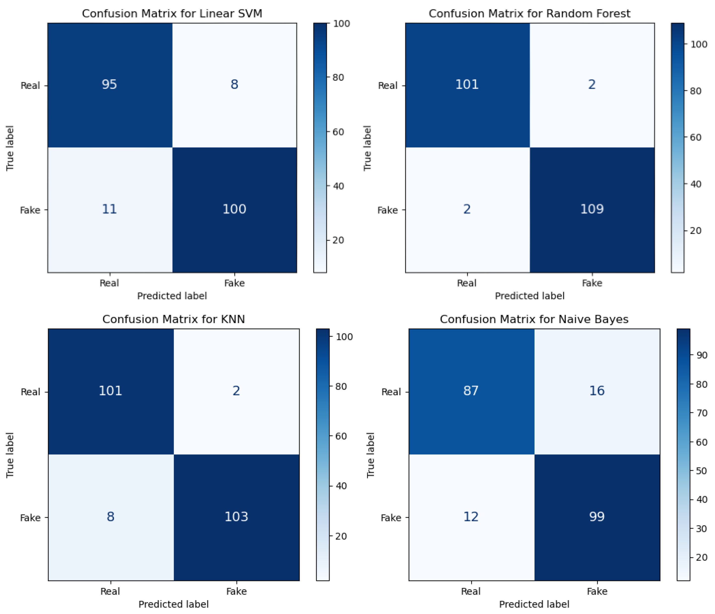
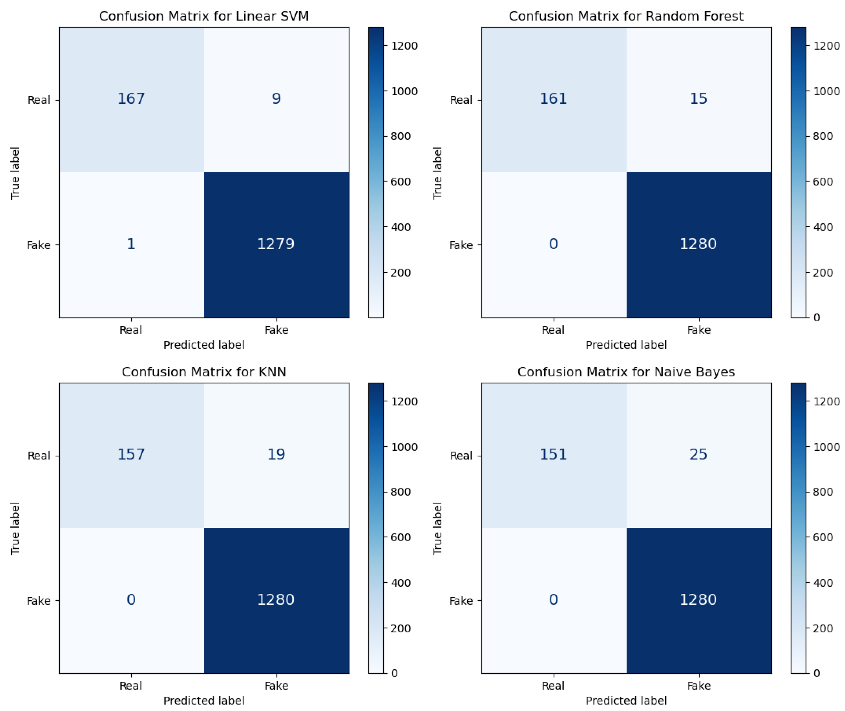
6.1. Results of the Classification of Deepfakes

In this work, we have used the F1 metric to evaluate the performance of our models, which combines precision and recall into a single value. The choice of this metric is based on its usefulness in scenarios with imbalanced data, as is the case of our dataset, where one class is represented in greater proportion than the other. By balancing the consideration of both false positives and false negatives, the F1 metric avoids favoring the prediction of the majority class, thereby capturing the overall performance of the model more accurately.

The summary of the F1 score results for each of the classifiers, together with their corresponding standard deviation for each of the two datasets, is presented in

Table 2. F1-scores and their corresponding standard deviation for each dataset.

Dataset	Classifier	F1-Score	Standard Deviation
WELIVE	Linear SVM	98.34%	0.36%
	Random Forest	97.41%	0.84%
	KNN	96.71%	0.82%
	Naive Bayes	95.53%	1.24%
HABLA	Linear SVM	93.67%	1.20%
	Random Forest	94.60%	1.63%
	KNN	94.01%	0.68%
	Naive Bayes	85.33%	1.29%

. From this table, it can be seen that, in general, the performance of the classifiers is higher for WELIVE than for HABLA. While for WELIVE, the Linear SVM classifier achieves the best F1 score with a value of $98.34$ and a low standard deviation of $0.36$, in the HABLA dataset, the Random Forest classifier stands out with the best F1 score of $94.60$, albeit with a relatively high standard deviation of $1.63$. On the other hand, the Naive Bayes classifier shows the lowest performance in both datasets, with an F1 score of $85.33$ and a standard deviation of $1.29$ for HABLA and an F1 of $95.53$ with a deviation of $1.24$ for WELIVE, the highest of all classifiers for that dataset. The results in this table indicate that there is a difference in the stability of classifier performance between the two datasets, reflected in the respective standard deviations. On the other hand, the difference between the classifier with the highest F1 value and the one with the lowest performance is $2.81$ in the WELIVE dataset. In the case of HABLA, three of the classifiers obtain similar F1 values; however, the difference between the classifier with the highest F1 and the one with the lowest performance reaches $9.27$. Due to these results, we can conclude that the detection of deepfakes is easier in WELIVE than in HABLA and we believe that this is due to the greater difficulty in creating them when the acoustic context is more complex. It should be noted, however, that the results of the two datasets are not directly comparable as both the number of samples used and the recording conditions of the audios are very different.

Figure 5 and Figure 6 present the confusion matrix corresponding to each classifier for both datasets. The main difference between these matrices lies in the fact that, for WELIVE, all the audios that are not correctly labeled correspond to real audios that were classified as false, with the exception of the linear SVM classifier, which, among the seven misclassified audios, records one false audio, erroneously labeled as real. On the other hand, when analyzing the confusion matrix of HABLA, it is observed that the percentage of misclassified audios, both false labeled as real and real labeled as false, is approximately balanced. Even for the KNN classifier, of the 10 misclassified audios, eight are fakes that were labeled as real. Since we have balanced the two classes in terms of the number of audios, these observations suggest that it is more difficult to trick a classifier into labeling fake audios as real when the deepfakes contain acoustic context.

Additionally, we have estimated the quality of both HABLA and WELIVE, using the model proposed by [54], which is designed to predict speech quality with a focus on distortions specific to communication networks. This model not only predicts overall speech quality but also evaluates specific dimensions such as Noise, Coloration, Discontinuity, and Loudness. The results show that for HABLA, the mean opinion score (MOS) of the audio is $4.37$, while for WELIVE it is $1.68$. This indicates that the audio corresponding to HABLA with a high MOS exhibits a significantly superior quality, which could favor the generation of deepfakes with a higher level of realism. In contrast, the audio from WELIVE with a low MOS shows significant deficiencies that will likely negatively impact the quality of the generated deepfakes.

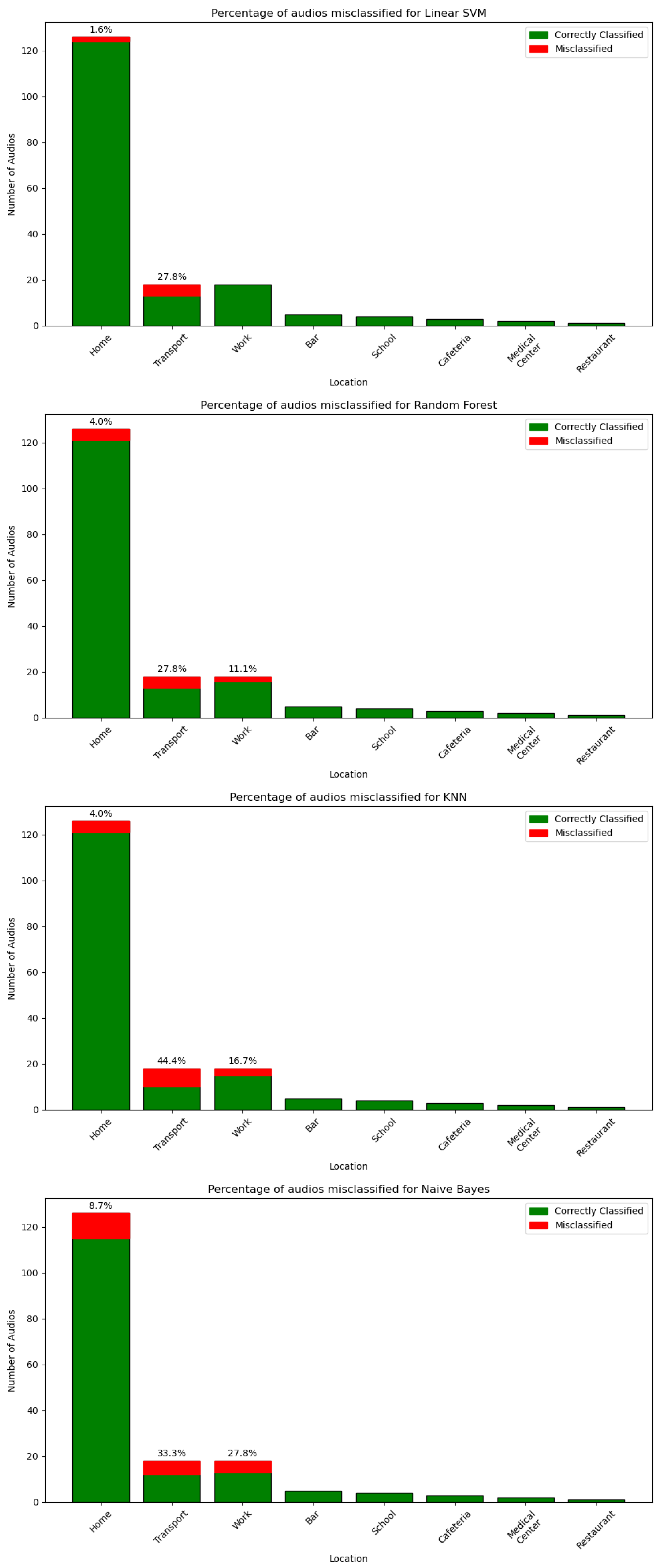
6.2. The Influence of the Acoustic Context

To analyze the factors that may influence detection, several aspects were evaluated. First, as detailed in Section 4, the acoustic context of each voice note was examined. The results regarding the percentage of audios misclassified based on their location are presented in

Table 3. Percentage of misclassified audios based on locations.

	Linear SVM	Random Forest	KNN	Naive Bayes
Home	28.57%	41.66%	31.25%	50%
Transport	71.42%	41.66%	50%	27.27%
Work	0%	16.66%	18.75%	27.27%
Bar	0%	0%	0%	0%
School	0%	0%	0%	0%
Cafeteria	0%	0%	0%	0%
Medical Center	0%	0%	0%	0%
Restaurant	0%	0%	0%	0%

. These results reveal a significant variability in classifier performance as a function of audio location. In particular, it is observed that in the locations Bar, School, Cafeteria, Medical Center and Restaurant, the percentage of misclassified audios is $0\%$, indicating perfect performance in these contexts for all classifiers. The Linear SVM classifier stands out for its flawless performance in the Work category, although it shows poor performance in Transport, with the highest percentage of errors. In contrast, the Naive Bayes classifier, despite its lower accuracy in Home, shows higher efficiency in Transport and Work, with the lowest percentage of errors in these categories. Analysis of the KNN results reveals low performance in Transport, where half of the classification errors are concentrated, while the other 50% is distributed between Home and Work. A similar pattern is observed in the Random Forest classifier, where almost half of the errors correspond to the Transport category. These results suggest that, with the exception of Naive Bayes, classifying audios in the Transport category is more challenging for the other classifiers. Figure 7 shows, for the four classifiers, the percentage of misclassified audios in each location relative to the total number of audios in that context. It is observed that in the Transport category, $27.7\%$ of the total number of audios in that context were misclassified by the Linear SVM and Random Forest classifiers, while in Naive Bayes this percentage amounts to $33.3\%$ and in KNN to $44.4\%$. It is important to note that this location analysis was carried out only for the real audio, since in the case of the synthetic audio, all locations were classified as Home.

6.3. The Influence of the User

Another aspect that was considered was the user to whom the voice memo corresponded. The percentages of incorrectly classified audios, according to the user, are shown in

Table 4. Percentage of misclassified audios based on the user.

	Linear SVM	Random Forest	KNN	Naive Bayes
V11O	28.57%	50%	37.50%	68.18%
T02	14.28%	0%	6.25%	4.54%
T03	0%	0%	0%	0%
T01	28.57%	16.66%	12.50%	4.54%
V134	0%	0%	0%	4.54%
P041	0%	0%	0%	0%
P007	28.57%	25%	18.75%	4.54%
T05	0%	0%	12.50%	4.54%
V104	0%	0%	0%	4.54%
V124	0%	0%	0%	0%
P008	0%	0%	0%	0%
V042	0%	8.33%	12.50%	4.54%
P059	0%	0%	0%	0%

. It shows that, for all classifiers, most of the audios that were not correctly labeled belong to the user V110. Likewise, in the cases of users T03, P041, V124, P008 and P059, all the classifiers manage to correctly label all the audios. As for the rest of the users, the classification errors are relatively evenly distributed. On the other hand, Figure 8 illustrates the percentage of misclassified audios in relation to the total number of audios belonging to each user. From that graph, it can be seen, for example, that in the case of the Naive Bayes classifier, almost one third of the audios of user V110 are misclassified. This suggests that, for certain users, the correct classification of the audio presents greater difficulties.

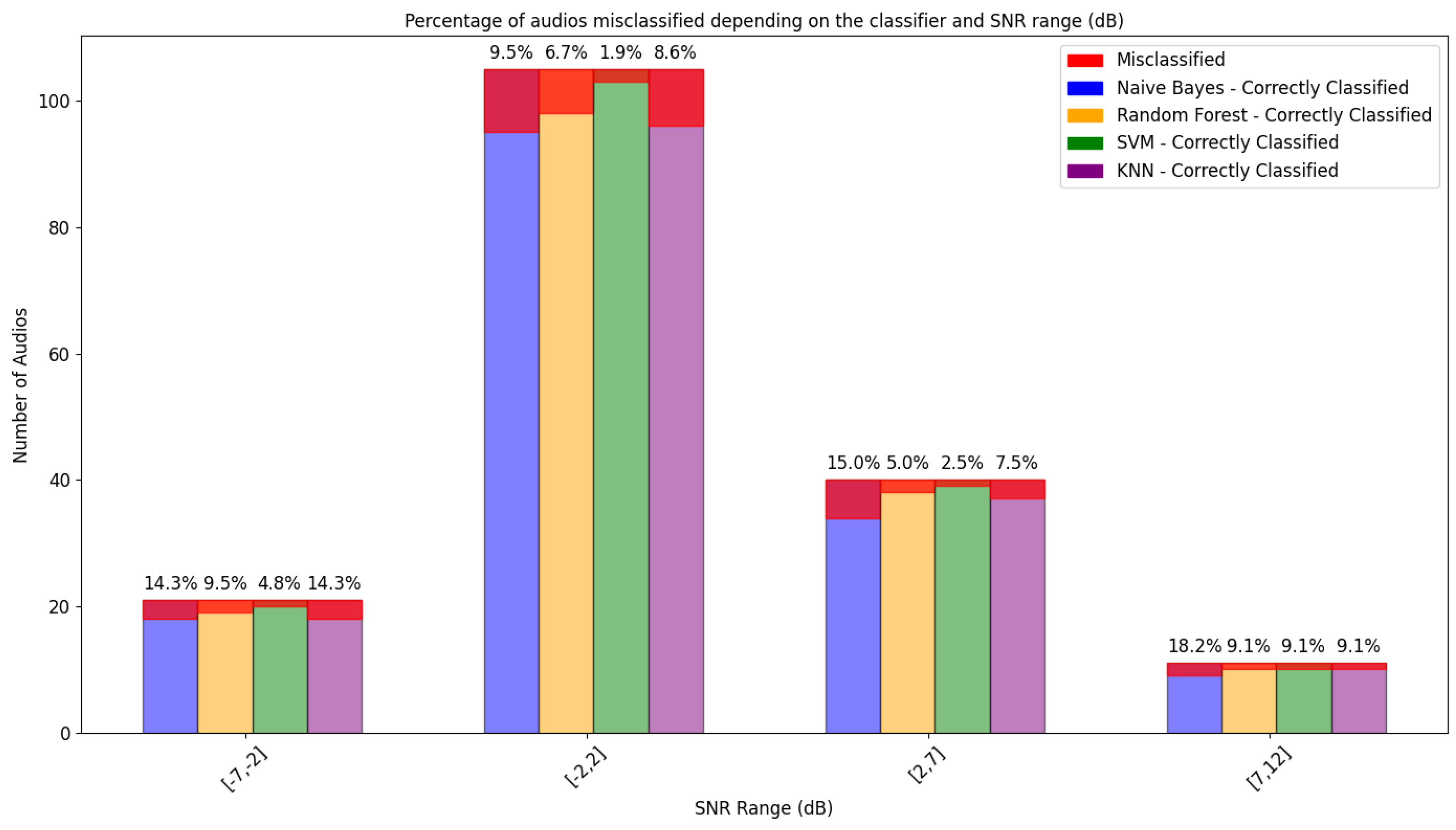
6.4. The Influence of the SNR

Figure 9 illustrates the variation of the percentage of hits as a function of the SNR of the audios. We can observe that most of the audio notes are in the [−2 dB, 2 dB] range. Although it is difficult to find clear trends in terms of the evolution of the SNR hit rate, we can observe that it is in the middle ranges ([−2 dB, 7dB]) when it is easier to detect deepfakes. The extreme values (ranges [−7 dB, 2 dB] and [7 dB, 12 dB]) have the highest number of misclassified samples. This occurs for all classifiers except for the Naive Bayes case, where the range ([2 dB, 7dB]) has a higher percentage of misclassified audios than the range [−7 dB, −2 dB]. From the results obtained, it can be observed that the SNR has a significant impact on the accuracy of the classifiers.

6.5. The Influence of Other Factors

Finally, the duration of the audios was ruled out as an influential factor, since the duration of the misclassified audios ranged approximately from $2.5$ s to $45.0$ s, similar to that of the correctly classified ones.

7. Conclusions

The focus of this paper is to identify and quantify the influence of different factors in the generation and detection of audio deepfakes in real-life unconstrained environments. In particular, we have analyzed the influence of first, the acoustic context type represented by eight different locations; second, the speaker and third, the signal-to-noise ratio.

We have concluded that deepfake detection models are more effective in the presence of real-life acoustic contexts such as in WELIVE, than in their absence like in HABLA, underlying the difficulties of state-of-the-art deepfake generators to reproduce realistic acoustic environments. Remarkably, the acoustic environment that facilitates the detection of deepfakes is transport. This finding underscores the importance of environmental features in the effectiveness of detection models and that these contexts influence the classification of audios. Moreover, there are some locations in our dataset that are underrepresented, where the detection is perfect, that need to be further investigated due to the difficulties in obtaining significant results with such few examples.

Regarding the influence of the user, we can also observe important variabilities, with V110 being the one that eases deepfake generation more, as can be observed by the higher number of errors in their detection. The connections to the preferred acoustic context in which the different subjects recorded speech should be further investigated.

Finally, our research on the influence of the SNR is not conclusive but the results hint that medium SNRs facilitate detection while very low or very high SNRs hinder it.

8. Future Work

Despite the progress made in our study, several restrictions remain to be addressed in future research. The main limitation of our project is the size of the dataset available; therefore, although the main results are significant attending to their standard deviations, some of the factors influencing the generation and detection could benefit from a larger dataset evaluation. Furthermore, it is still unclear whether deepfakes in WELIVE are more easily detected compared to those in HABLA, due to the lower quality in the generation of these audios, or due to higher ease of detection when a singular acoustic context is present. As part of future lines of work, we propose the development of models that integrate contextual and personalized features in order to improve both the generation and detection of audios in various scenarios. It would be valuable to explore other acoustic contexts and consider additional factors, such as the different emotions reflected in the voice, to create a more realistic approach. Another important aspect to improve is the quality of the audio generation since when using StarGANv2-vc, trained in controlled environments, the recordings obtained with our data do not reach an optimal level of realism. Also, training the PaSST model to identify the locations of the deepfakes, and not only of the real audios, is another goal we set ourselves. In addition, we plan to expand the dataset to include male voices, since our current study has focused exclusively on female voices. We are also interested in exploring the use of deepfakes with sentences not uttered by female users but with their voices, with the aim of detecting such cases, as they could be used as false evidence in a trial. In addition, we believe that it could be beneficial to conduct a subjective evaluation in which some people listen to the audios and determine whether they perceive them to be genuine or fake, in order to compare the classifiers’ hit rate with that of the users. Finally, evaluating the performance of the classifiers using full audio recordings, as described in Section 3, is part of our ongoing work. The goal is to analyze its effectiveness in more complex scenarios. To facilitate this analysis, we plan to implement a speaker recognition system, which will allow us to more accurately and efficiently identify the segments that correspond to the primary user. This approach will provide a more rigorous evaluation of the classifiers’ ability to handle a greater diversity of data and acoustic contexts.

References

1. Martínez-Serrano, A.; Montero-Ramírez, C.; Peláez-Moreno, C. The Influence of Acoustic Context on the Generation and Detection of Audio Deepfakes. In Proceedings of the Iberspeech 2024, Aveiro, Portugal, 11–13 November 2024. [Google Scholar]
2. Zhang, J.; Tao, D. Empowering Things with Intelligence: A Survey of the Progress, Challenges, and Opportunities in Artificial Intelligence of Things. IEEE Internet Things J. 2021, 8, 7789–7817. [Google Scholar] [CrossRef]
3. Gambín, Á.F.; Yazidi, A.; Vasilakos, A.; Haugerud, H.; Djenouri, Y. Deepfakes: Current and future trends. Artif. Intell. Rev. 2024, 57, 64. [Google Scholar] [CrossRef]
4. Hu, H.R.; Song, Y.; Liu, Y.; Dai, L.R.; McLoughlin, I.; Liu, L. Domain robust deep embedding learning for speaker recognition. In Proceedings of the ICASSP 2022—2022 IEEE International Conference on Acoustics, Speech and Signal Processing (ICASSP), Singapore, 23–27 May 2022; pp. 7182–7186. [Google Scholar]
5. Mcuba, M.; Singh, A.; Ikuesan, R.A.; Venter, H. The effect of deep learning methods on deepfake audio detection for digital investigation. Procedia Comput. Sci. 2023, 219, 211–219. [Google Scholar] [CrossRef]
6. Miranda Calero, J.A.; Rituerto-González, E.; Luis-Mingueza, C.; Canabal Benito, M.F.; Ramírez Bárcenas, A.; Lanza Gutiérrez, J.M.; Peláez-Moreno, C.; López-Ongil, C. Bindi: Affective Internet of Things to Combat Gender-Based Violence. IEEE Internet Things J. 2022, 9, 21174–21193. [Google Scholar] [CrossRef]
7. Salvi, D.; Hosler, B.; Bestagini, P.; Stamm, M.C.; Tubaro, S. TIMIT-TTS: A text-to-speech dataset for multimodal synthetic media detection. IEEE Access 2023, 11, 50851–50866. [Google Scholar] [CrossRef]
8. Sun, C.; Jia, S.; Hou, S.; Lyu, S. Ai-synthesized voice detection using neural vocoder artifacts. In Proceedings of the IEEE/CVF Conference on Computer Vision and Pattern Recognition, Vancouver, BC, Canada, 17–24 June 2023; pp. 904–912. [Google Scholar]
9. Toda, T.; Chen, L.H.; Saito, D.; Villavicencio, F.; Wester, M.; Wu, Z.; Yamagishi, J. The Voice Conversion Challenge 2016. In Proceedings of the Interspeech, San Francisco, CA, USA, 8–12 September 2016; Volume 2016, pp. 1632–1636. [Google Scholar]
10. Ping, W.; Peng, K.; Gibiansky, A.; Arik, S.O.; Kannan, A.; Narang, S.; Raiman, J.; Miller, J. Deep voice 3: Scaling text-to-speech with convolutional sequence learning. arXiv 2017, arXiv:1710.07654. [Google Scholar]
11. Ren, Y.; Hu, C.; Tan, X.; Qin, T.; Zhao, S.; Zhao, Z.; Liu, T.Y. Fastspeech 2: Fast and high-quality end-to-end text to speech. arXiv 2020, arXiv:2006.04558. [Google Scholar]
12. Kaneko, T.; Kameoka, H.; Tanaka, K.; Hojo, N. Cyclegan-vc2: Improved cyclegan-based non-parallel voice conversion. In Proceedings of the ICASSP 2019—2019 IEEE International Conference on Acoustics, Speech and Signal Processing (ICASSP), Brighton, UK, 12–17 May 2019; pp. 6820–6824. [Google Scholar]
13. Li, Y.A.; Zare, A.; Mesgarani, N. Starganv2-vc: A diverse, unsupervised, non-parallel framework for natural-sounding voice conversion. arXiv 2021, arXiv:2107.10394. [Google Scholar]
14. Yamamoto, R.; Song, E.; Kim, J.M. Parallel WaveGAN: A Fast Waveform Generation Model Based on Generative Adversarial Networks with Multi-Resolution Spectrogram. arXiv 2020, arXiv:1910.11480. [Google Scholar]
15. Ballesteros, D.M.; Rodriguez, Y.; Renza, D. A dataset of histograms of original and fake voice recordings (H-Voice). Data Brief 2020, 29, 105331. [Google Scholar] [CrossRef]
16. Khalid, H.; Tariq, S.; Kim, M.; Woo, S.S. FakeAVCeleb: A novel audio-video multimodal deepfake dataset. arXiv 2021, arXiv:2108.05080. [Google Scholar]
17. Yi, J.; Bai, Y.; Tao, J.; Ma, H.; Tian, Z.; Wang, C.; Wang, T.; Fu, R. Half-truth: A partially fake audio detection dataset. arXiv 2021, arXiv:2104.03617. [Google Scholar]
18. Barni, M.; Campisi, P.; Delp, E.J.; Doërr, G.; Fridrich, J.; Memon, N.; Pérez-González, F.; Rocha, A.; Verdoliva, L.; Wu, M. Information Forensics and Security: A quarter-century-long journey. IEEE Signal Process. Mag. 2023, 40, 67–79. [Google Scholar] [CrossRef]
19. Kalpokas, I.; Kalpokiene, J. Deepfakes: A Realistic Assessment of Potentials, Risks, and Policy Regulation; Springer: Berlin/Heidelberg, Germany, 2022. [Google Scholar]
20. Tolosana, R.; Vera-Rodriguez, R.; Fierrez, J.; Morales, A.; Ortega-Garcia, J. Deepfakes and beyond: A survey of face manipulation and fake detection. Inf. Fusion 2020, 64, 131–148. [Google Scholar] [CrossRef]
21. Martín-Doñas, J.M.; Álvarez, A. The vicomtech audio deepfake detection system based on wav2vec2 for the 2022 add challenge. In Proceedings of the ICASSP 2022—2022 IEEE International Conference on Acoustics, Speech and Signal Processing (ICASSP), Singapore, 23–27 May 2022; pp. 9241–9245. [Google Scholar]
22. Yi, J.; Tao, J.; Fu, R.; Yan, X.; Wang, C.; Wang, T.; Zhang, C.Y.; Zhang, X.; Zhao, Y.; Ren, Y.; et al. Add 2023: The second audio deepfake detection challenge. arXiv 2023, arXiv:2305.13774. [Google Scholar]
23. Rodríguez-Ortega, Y.; Ballesteros, D.M.; Renza, D. A machine learning model to detect fake voice. In International Conference on Applied Informatics; Springer: Berlin/Heidelberg, Germany, 2020; pp. 3–13. [Google Scholar]
24. Singh, A.K.; Singh, P. Detection of ai-synthesized speech using cepstral & bispectral statistics. In Proceedings of the 2021 IEEE 4th International Conference on Multimedia Information Processing and Retrieval (MIPR), Tokyo, Japan, 8–10 September 2021; pp. 412–417. [Google Scholar]
25. Li, X.; Li, N.; Weng, C.; Liu, X.; Su, D.; Yu, D.; Meng, H. Replay and synthetic speech detection with res2net architecture. In Proceedings of the ICASSP 2021—2021 IEEE International Conference on Acoustics, Speech and Signal Processing (ICASSP), Toronto, ON, Canada, 6–11 June 2021; pp. 6354–6358. [Google Scholar]
26. Gomez-Alanis, A.; Peinado, A.M.; Gonzalez, J.A.; Gomez, A.M. A light convolutional GRU-RNN deep feature extractor for ASV spoofing detection. In Proceedings of the Interspeech, Graz, Austria, 15–19 September 2019; Volume 2019, pp. 1068–1072. [Google Scholar]
27. Subramani, N.; Rao, D. Learning efficient representations for fake speech detection. In Proceedings of the AAAI Conference on Artificial Intelligence, New York, NY, USA, 7–12 February 2020; Volume 34, pp. 5859–5866. [Google Scholar]
28. Ballesteros, D.M.; Rodriguez-Ortega, Y.; Renza, D.; Arce, G. Deep4SNet: Deep learning for fake speech classification. Expert Syst. Appl. 2021, 184, 115465. [Google Scholar] [CrossRef]
29. Xie, Z.; Li, B.; Xu, X.; Liang, Z.; Yu, K.; Wu, M. FakeSound: Deepfake General Audio Detection. arXiv 2024, arXiv:2406.08052. [Google Scholar]
30. Xu, X.; Ma, Z.; Wu, M.; Yu, K. Towards Weakly Supervised Text-to-Audio Grounding. arXiv 2024, arXiv:2401.02584. [Google Scholar] [CrossRef]
31. Liu, H.; Chen, K.; Tian, Q.; Wang, W.; Plumbley, M.D. AudioSR: Versatile audio super-resolution at scale. In Proceedings of the ICASSP 2024-2024 IEEE International Conference on Acoustics, Speech and Signal Processing (ICASSP), Seoul, Republic of Korea, 14–19 April 2024; pp. 1076–1080. [Google Scholar]
32. Kim, C.D.; Kim, B.; Lee, H.; Kim, G. Audiocaps: Generating captions for audios in the wild. In Proceedings of the 2019 Conference of the North American Chapter of the Association for Computational Linguistics: Human Language Technologies, Volume 1 (Long and Short Papers), Minneapolis, MN, USA, 2–7 June 2019; pp. 119–132. [Google Scholar]
33. Rituerto González, E. Multimodal Affective Computing in Wearable Devices with Applications in the Detection of Gender-Based Violence; Programa de Doctorado en Multimedia y Comunicaciones, Universidad Carlos III de Madrid: Madrid, Spain, 2023. [Google Scholar]
34. Montero-Ramírez, C.; Rituerto-González, E.; Peláez-Moreno, C. Evaluation of Automatic Embeddings for Supervised Soundscape Classification in-the-wild. In Proceedings of the Iberspeech 2024, Aveiro, Portugal, 11–13 November 2024. [Google Scholar]
35. Rituerto-González, E.; Miranda, J.A.; Canabal, M.F.; Lanza-Gutiérrez, J.M.; Peláez-Moreno, C.; López-Ongil, C. A Hybrid Data Fusion Architecture for BINDI: A Wearable Solution to Combat Gender-Based Violence. In Multimedia Communications, Services and Security; Dziech, A., Mees, W., Czyżewski, A., Eds.; Communications in Computer and Information Science; Springer International Publishing: Cham, Switzerland, 2020; pp. 223–237. [Google Scholar]
36. Montero-Ramírez, C.; Rituerto-González, E.; Peláez-Moreno, C. Building Artificial Situational Awareness: Soundscape Classification in Daily-life Scenarios of Gender based Violence Victims. Eng. Appl. Artif. Intell. 2024; submitted for publication. [Google Scholar]
37. Kum, S.; Nam, J. Joint detection and classification of singing voice melody using convolutional recurrent neural networks. Appl. Sci. 2019, 9, 1324. [Google Scholar] [CrossRef]
38. Veaux, C.; Yamagishi, J.; MacDonald, K. Superseded-CSTR VCTK Corpus: English Multi-Speaker Corpus for CSTR Voice Cloning Toolkit. 2016. Available online: http://datashare.is.ed.ac.uk/handle/10283/2651 (accessed on 13 May 2024).
39. Rabiner, L.; Schafer, R. Theory and Applications of Digital Speech Processing, 1st ed.; Prentice Hall Press: Hoboken, NJ, USA, 2010. [Google Scholar]
40. Cortes, C.; Vapnik, V. Support-Vector Networks. Mach. Learn. 1995, 20, 273–297. [Google Scholar] [CrossRef]
41. Breiman, L. Random Forests. Mach. Learn. 2001, 45, 5–32. [Google Scholar] [CrossRef]
42. Cover, T.; Hart, P. Nearest Neighbor Pattern Classification. IEEE Trans. Inf. Theory 1967, 13, 21–27. [Google Scholar] [CrossRef]
43. Friedman, N.; Geiger, D.; Goldszmidt, M. Bayesian Network Classifiers. Mach. Learn. 1997, 29, 131–163. [Google Scholar] [CrossRef]
44. Koutini, K.; Schlüter, J.; Eghbal-Zadeh, H.; Widmer, G. Efficient training of audio transformers with patchout. arXiv 2021, arXiv:2110.05069. [Google Scholar]
45. Park, D.S.; Chan, W.; Zhang, Y.; Chiu, C.C.; Zoph, B.; Cubuk, E.D.; Le, Q.V. Specaugment: A simple data augmentation method for automatic speech recognition. arXiv 2019, arXiv:1904.08779. [Google Scholar]
46. Gemmeke, J.F.; Ellis, D.P.; Freedman, D.; Jansen, A.; Lawrence, W.; Moore, R.C.; Plakal, M.; Ritter, M. Audio set: An ontology and human-labeled dataset for audio events. In Proceedings of the 2017 IEEE International Conference on Acoustics, Speech and Signal Processing (ICASSP), New Orleans, LA, USA, 5–9 March 2017; pp. 776–780. [Google Scholar]
47. Gong, Y.; Chung, Y.A.; Glass, J. Ast: Audio spectrogram transformer. arXiv 2021, arXiv:2104.01778. [Google Scholar]
48. Bredin, H.; Laurent, A. End-to-end speaker segmentation for overlap-aware resegmentation. In Proceedings of the Interspeech 2021, Brno, Czech Republic, 30 August–3 September 2021. [Google Scholar]
49. Tamayo Flórez, P.A.; Manrique, R.; Pereira Nunes, B. HABLA: A Dataset of Latin American Spanish Accents for Voice Anti-spoofing. In Proceedings of the Interspeech, Dublin, Ireland, 20–24 August 2023; pp. 1963–1967. [Google Scholar] [CrossRef]
50. Park, K.; Mulc, T. CSS10: A Collection of Single Speaker Speech Datasets for 10 Languages. arXiv 2019, arXiv:1903.11269. [Google Scholar]
51. Guevara-Rukoz, A.; Demirsahin, I.; He, F.; Chu, S.H.C.; Sarin, S.; Pipatsrisawat, K.; Gutkin, A.; Butryna, A.; Kjartansson, O. Crowdsourcing Latin American Spanish for Low-Resource Text-to-Speech. In Proceedings of the Twelfth Language Resources and Evaluation Conference, Marseille, France, 11–16 May 2020; Calzolari, N., Béchet, F., Blache, P., Choukri, K., Cieri, C., Declerck, T., Goggi, S., Isahara, H., Maegaard, B., Mariani, J., et al., Eds.; European Language Resources Association: Paris, France, 2020; pp. 6504–6513. [Google Scholar]
52. Popov, V.; Vovk, I.; Gogoryan, V.; Sadekova, T.; Kudinov, M.; Wei, J. Diffusion-based voice conversion with fast maximum likelihood sampling scheme. arXiv 2021, arXiv:2109.13821. [Google Scholar]
53. Pedregosa, F.; Varoquaux, G.; Gramfort, A.; Michel, V.; Thirion, B.; Grisel, O.; Blondel, M.; Prettenhofer, P.; Weiss, R.; Dubourg, V.; et al. Scikit-learn: Machine Learning in Python. J. Mach. Learn. Res. 2011, 12, 2825–2830. [Google Scholar]
54. Mittag, G.; Naderi, B.; Chehadi, A.; Möller, S. NISQA: A deep CNN-self-attention model for multidimensional speech quality prediction with crowdsourced datasets. arXiv 2021, arXiv:2104.09494. [Google Scholar]
Figure 1. Pipeline of the process followed to generate and detect deepfakes. WELIVE audio notes are used as source audio whilst a gender-balanced selection from VCTK is employed as reference. The StarGANv2-VC model provides a set of fake audio to which we add the original non-fake audios. A data resampling method is employed on the dataset to avoid unwanted effects on the classifier models due to imbalance.
Applsci 15 00558 g001
Figure 2. Influential factors in the generation and detection of audio deepfakes. The acoustic context and signal-to-noise ratio of the non-fake audios are estimated with a transformer-based model (PaSST) and a Voice Activity Detector (VAD), respectively. The coded identity (anonymized) of the users is already available from the dataset metadata.
Applsci 15 00558 g002
Figure 3. StarGANv2-VC framework (adapted from [13]). X src is the source input, X ref is the reference input that contains the style information, and X ^ represents the converted mel-spectrogram. h x , F conv and s denote the latent feature of the source, the F O feature from convolutional layers of the source, and the style code of the reference in the target domain, respectively.
Applsci 15 00558 g003
Figure 4. The Patchout transformer (PaSST) architecture (extracted from [44]).
Applsci 15 00558 g004
Figure 5. Confusion matrix of the different classifiers for the HABLA dataset. Each matrix illustrates the classifier’s performance in terms of true positives, false positives, true negatives, and false negatives. The classifiers analyzed are SVM, Random Forest, KNN, and Naive Bayes.
Applsci 15 00558 g005
Figure 6. Confusion matrix of the different classifiers for the WELIVE dataset. Each matrix illustrates the classifier’s performance in terms of true positives, false positives, true negatives, and false negatives. The classifiers analyzed are SVM, Random Forest, KNN, and Naive Bayes. This is the result of the accumulation of all the results of the eight balanced partitions as explained in the text.
Applsci 15 00558 g006
Figure 7. Percentage of audios misclassified for each classifier by location. The values displayed in red represent the percentage of audio samples incorrectly classified relative to the total number of samples for that location. For example, for Naive Bayes, in the “Home” location, if the classifier displays 8.7% in red, it means that 8.7% of the total audio samples in that category are misclassified.
Applsci 15 00558 g007
Figure 8. Percentage of audio misclassified for each classifier by user. The values displayed in red represent the percentage of audio samples incorrectly classified relative to the total number of samples for that user. For example, for Naive Bayes, for user V110, if the classifier displays 28.8% in red, it means that 28.8% of the total audio samples for that user are misclassified.
Applsci 15 00558 g008
Figure 9. Percentage of misclassified audio samples based on four distinct ranges of estimated signal-to-noise ratio (SNR). Each classifier is represented by a different color, and the values in red indicate the percentage of misclassified audio samples relative to the total number of samples in that SNR interval. The represented ranges are [−7, −2] dB, [−2, 2] dB, [2, 7] dB, and [7, 12] dB.
Applsci 15 00558 g009