
A Case Study of Using Numerical Analysis to Assess the Slope Stability of National Freeways in Northern Taiwan †


Abstract
:1. Introduction
2. Literature Review
2.1. Factors Affecting Slope Stability
- Geological material: The slope stratum is mainly composed of single or multiple geological materials. The cementation, particle size, and composition of the geological materials directly affect the stability of the slope.
- Geological structure: Weak planes (such as strike and dip angle) and slope surfaces (such as dip slope, anti-dip slope, and cross-dip) are the main factors affecting slope stability. Other geological structures, such as faults, joints, folds, layers, and other discontinuous surfaces, transform the slope’s rock and soil into discontinued or fragmented stones. These structures reduce rock and soil strength and increase weathering, affecting the slope’s stability.
- Topographic and environmental conditions: Topography includes the slope’s general form and rough surface terrain. While slope terrain has its own height and gradient, surface terrain relates to the characteristics of the geological structure. Groundwater, earthquakes, and rainfall are examples of environmental elements that affect slope stability.
- Engineering aspects: Slope stability is affected directly or indirectly by human factors such as freeways, tunnel excavation, blasting, overdevelopment of slopes, substandard building or site selection, poor slope drainage systems, and inadequate maintenance of protective structures.
- Class A slope: Slopes classified as class A exhibit clear indications of instability. Appropriate actions must be implemented right away, and cooperation with careful observation and monitoring is needed.
- Class B slope: Due to the possible indication of instability, additional patrols, monitoring, maintenance, reinforcing, and remediation are needed.
- Class C slope: The slope needs regular patrol or maintenance, with monitoring as necessary, even if there are no obvious signs of instability.
- Class D slope: Patrolling is still necessary, even though it is steady.
2.2. Prediction of Slope Stability
3. Overview of the Cases Studied
4. Numerical Analysis Software and Methods Used
4.1. PLAXIS 2D Program
4.2. Soil Material Combination Law
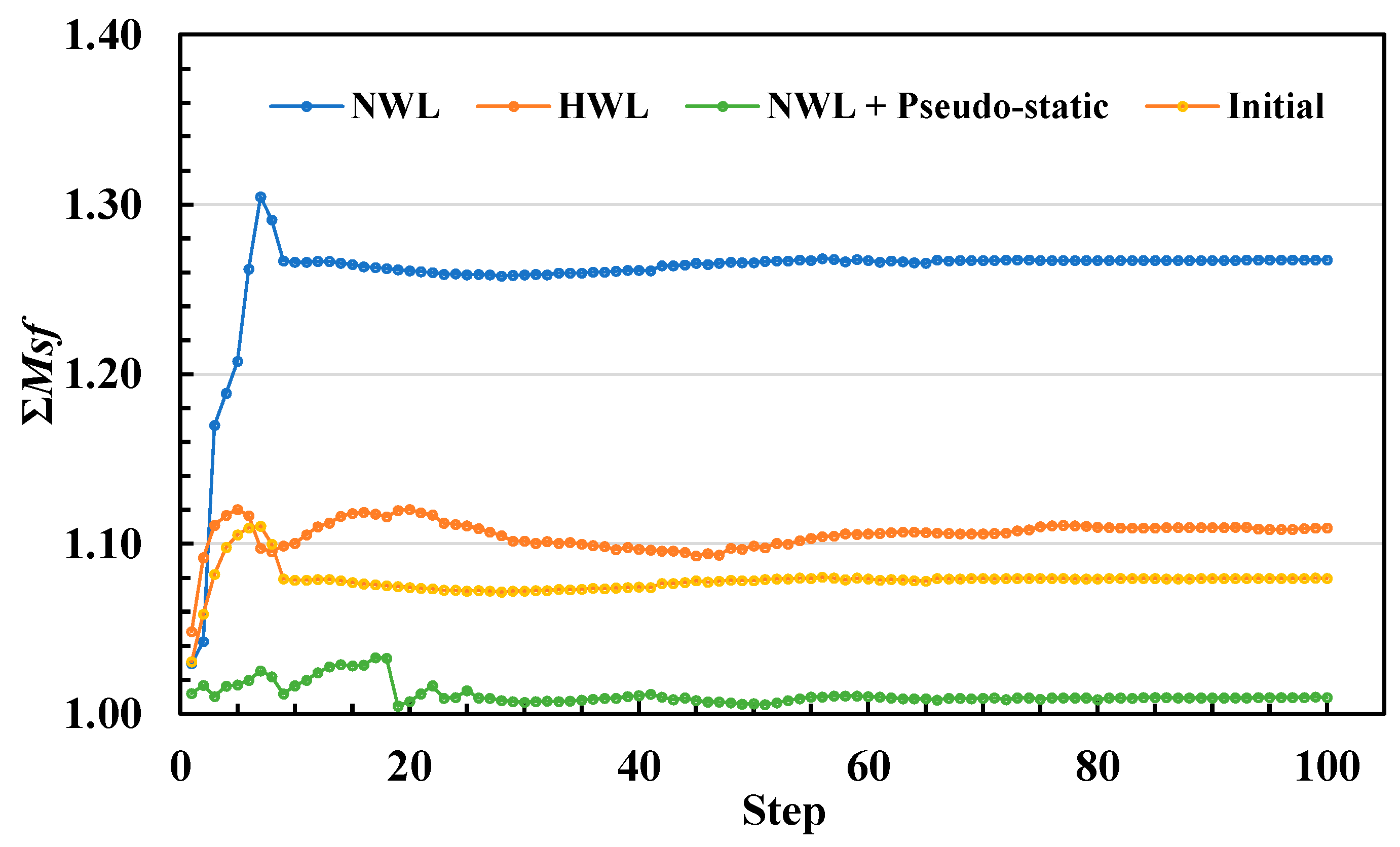
4.3. Safety Calculation
4.4. The Process of Establishing Numerical Models
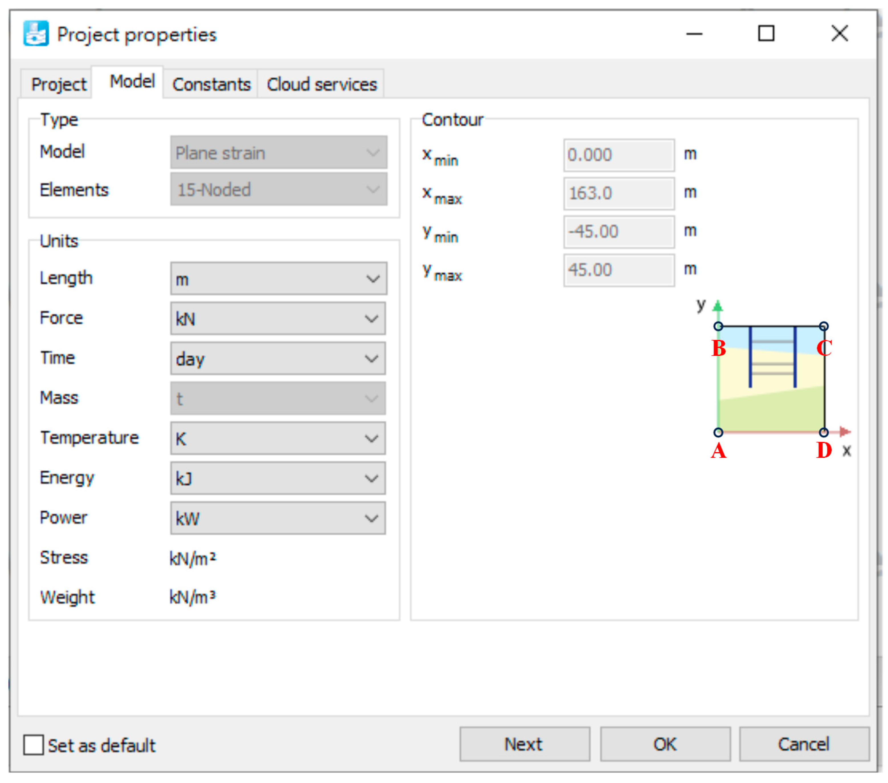
4.4.1. Model Boundary Conditions
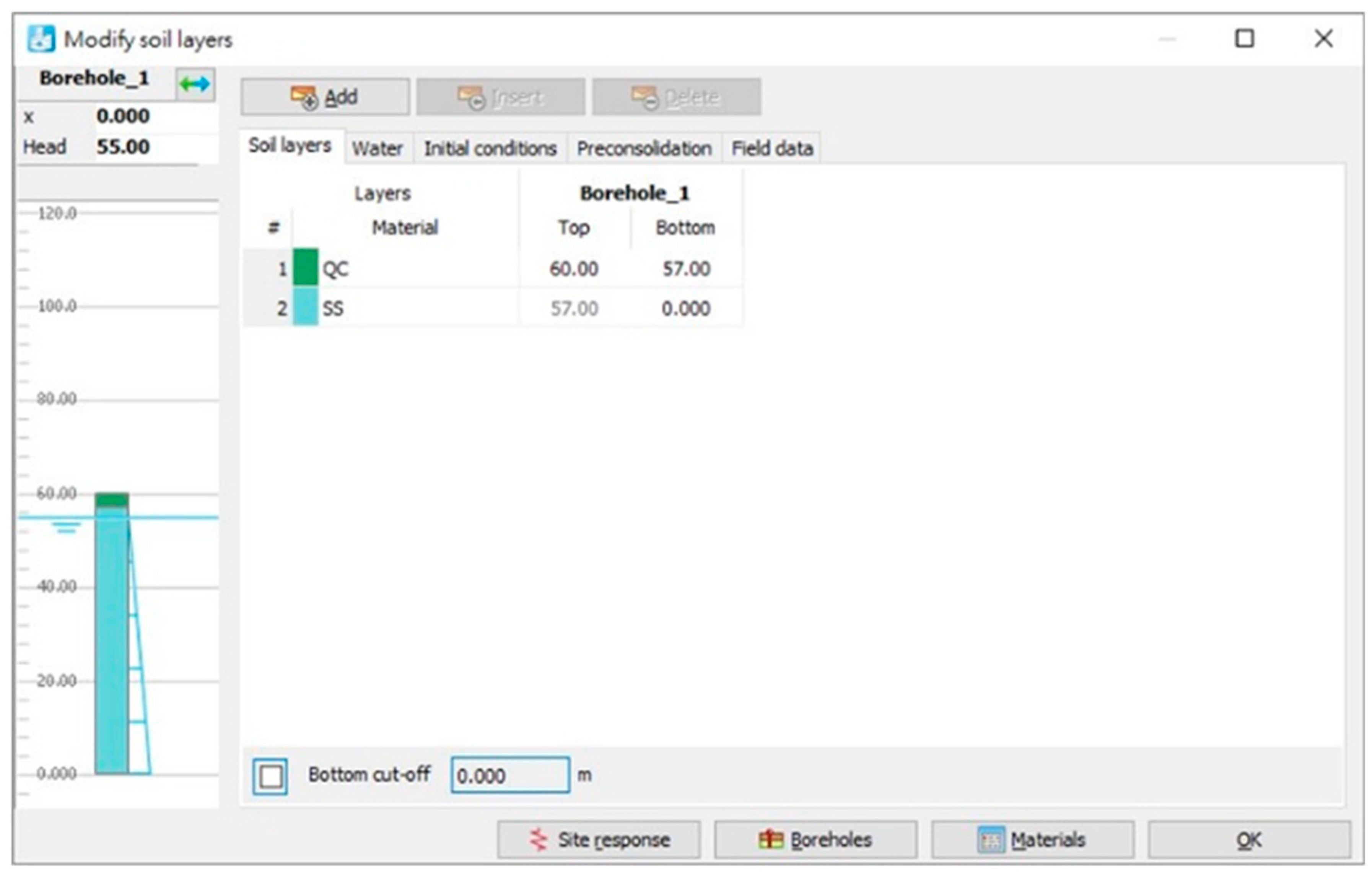
4.4.2. Soil Parameters and Groundwater Levels of Soil Layers
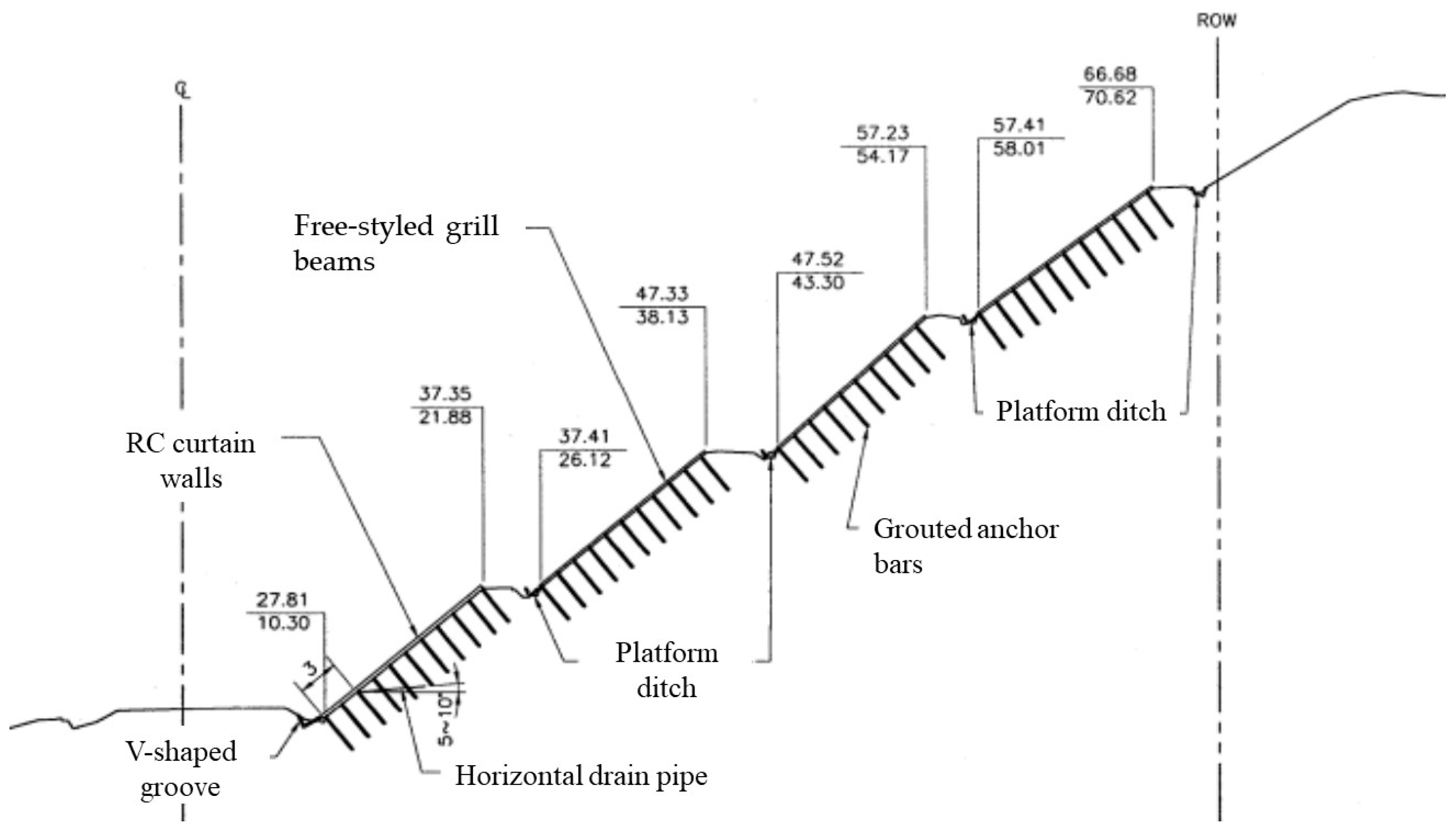
4.4.3. Structural Settings and Material Parameters
4.4.4. Generation of Mesh
4.4.5. Hydraulic Conditions
5. Numerical Analysis Results and Discussion
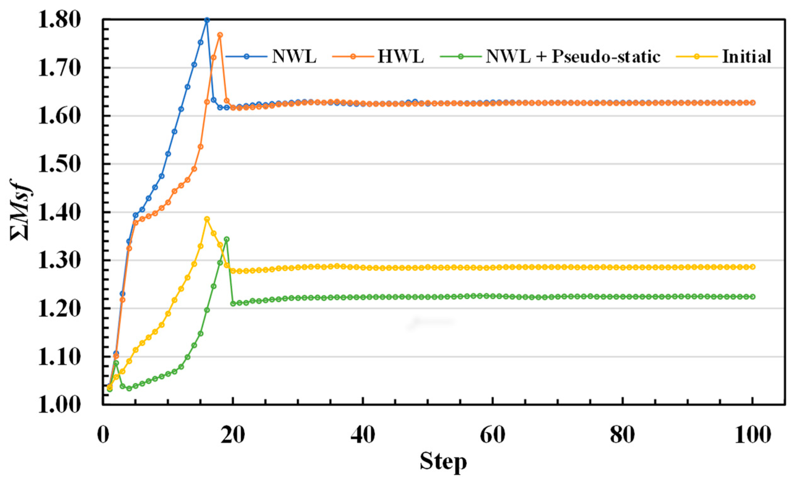
5.1. Normal Groundwater Level and High Groundwater Level
5.2. Seismic Loading in the Pseudo-Static Analysis
5.3. PLAXIS Analysis
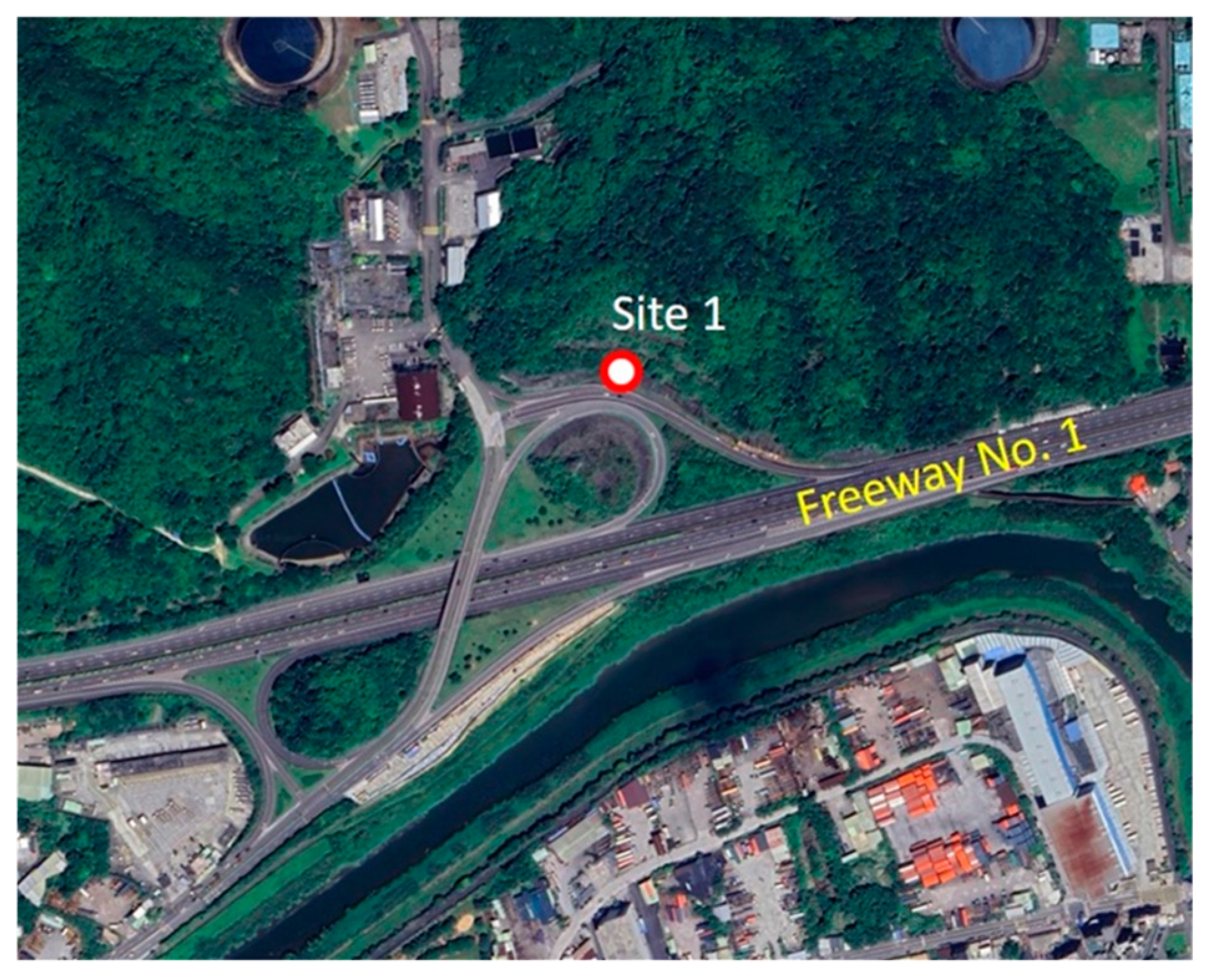
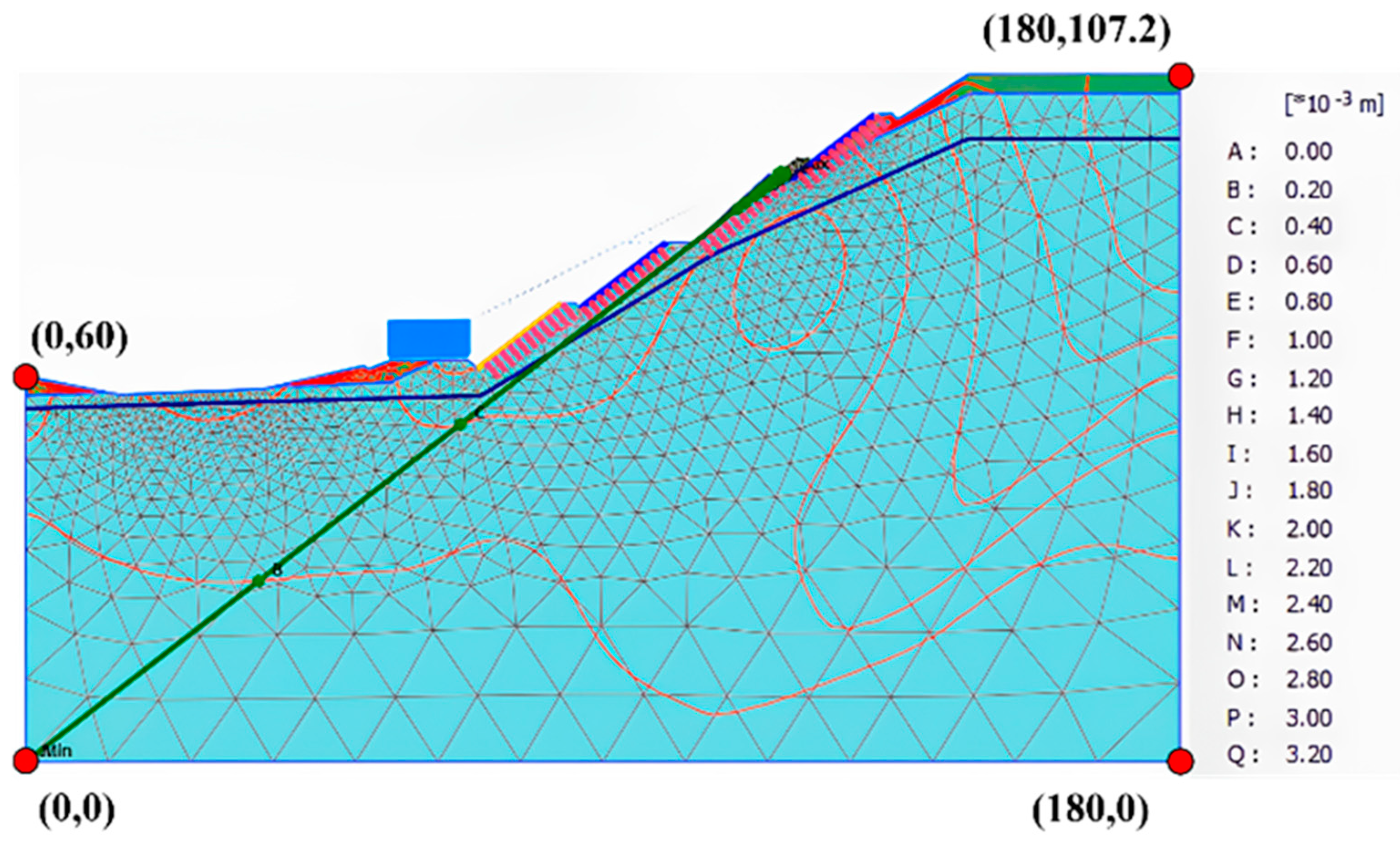
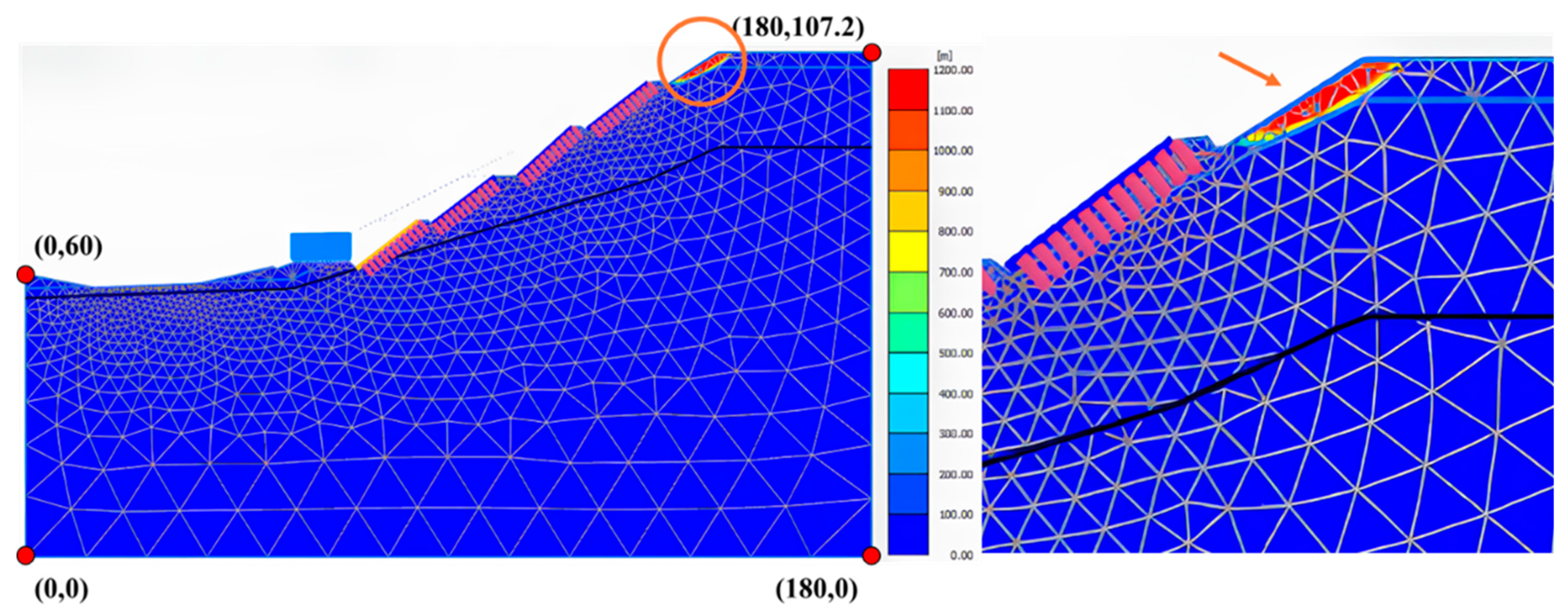
5.3.1. Case Simulation of Site 1
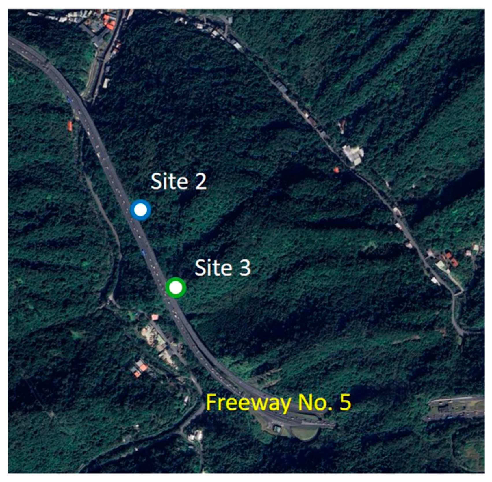
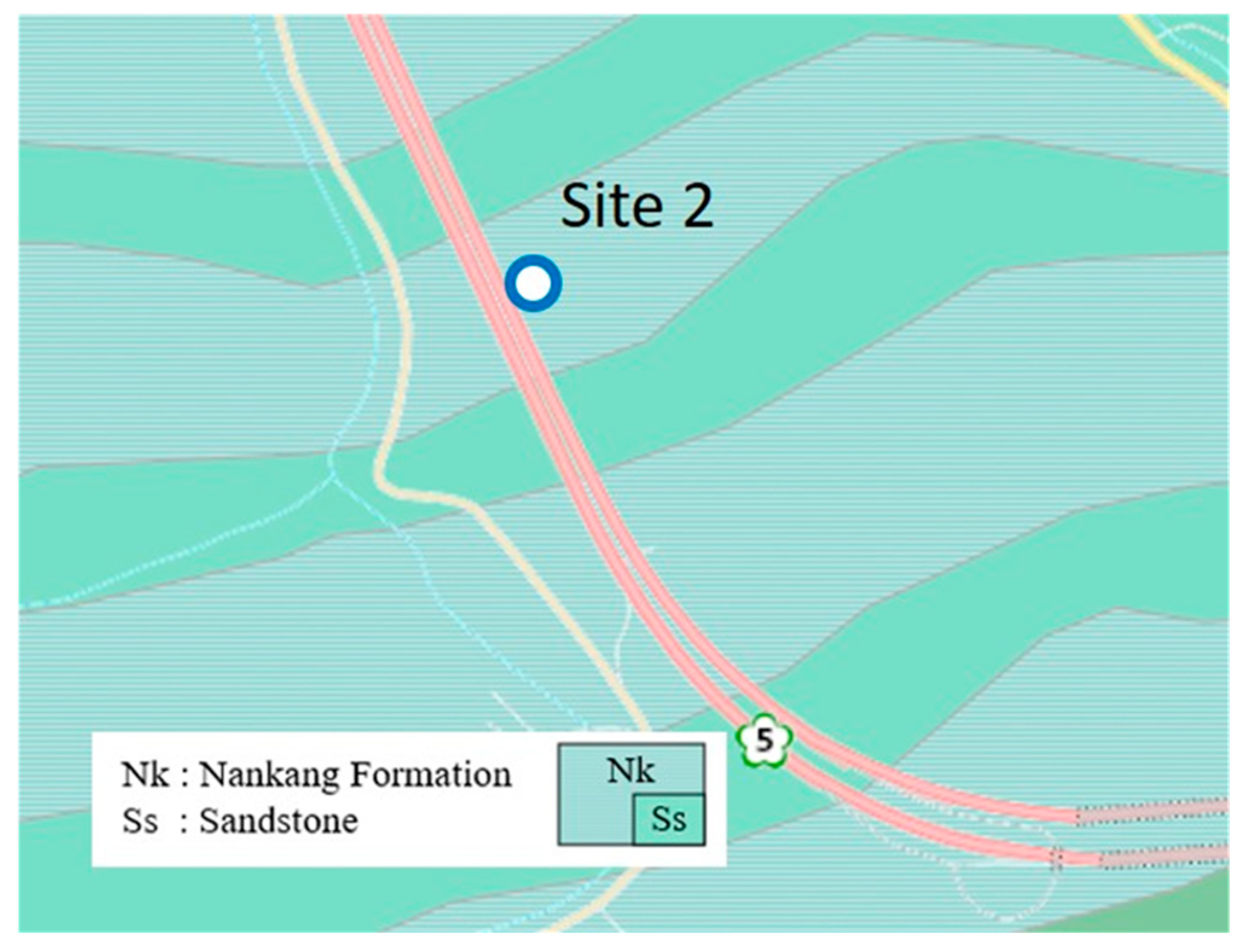
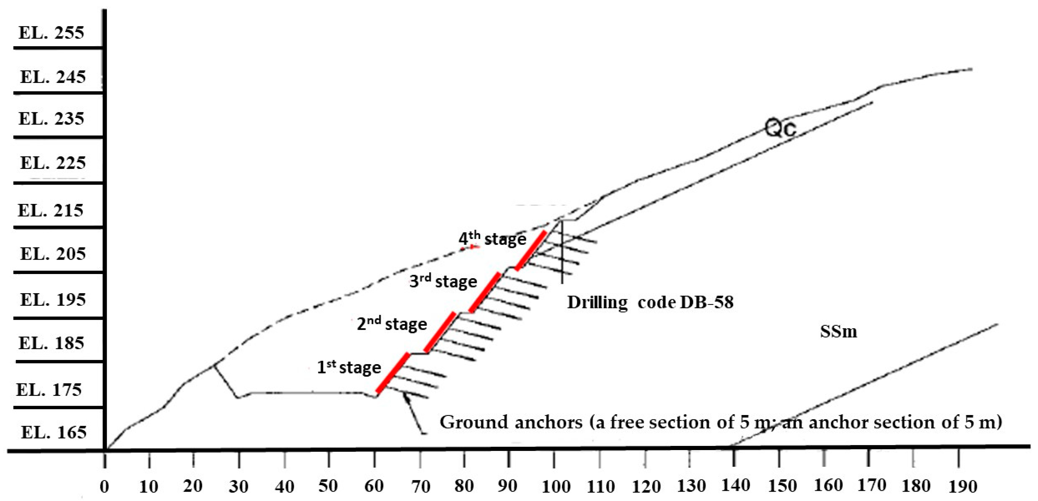
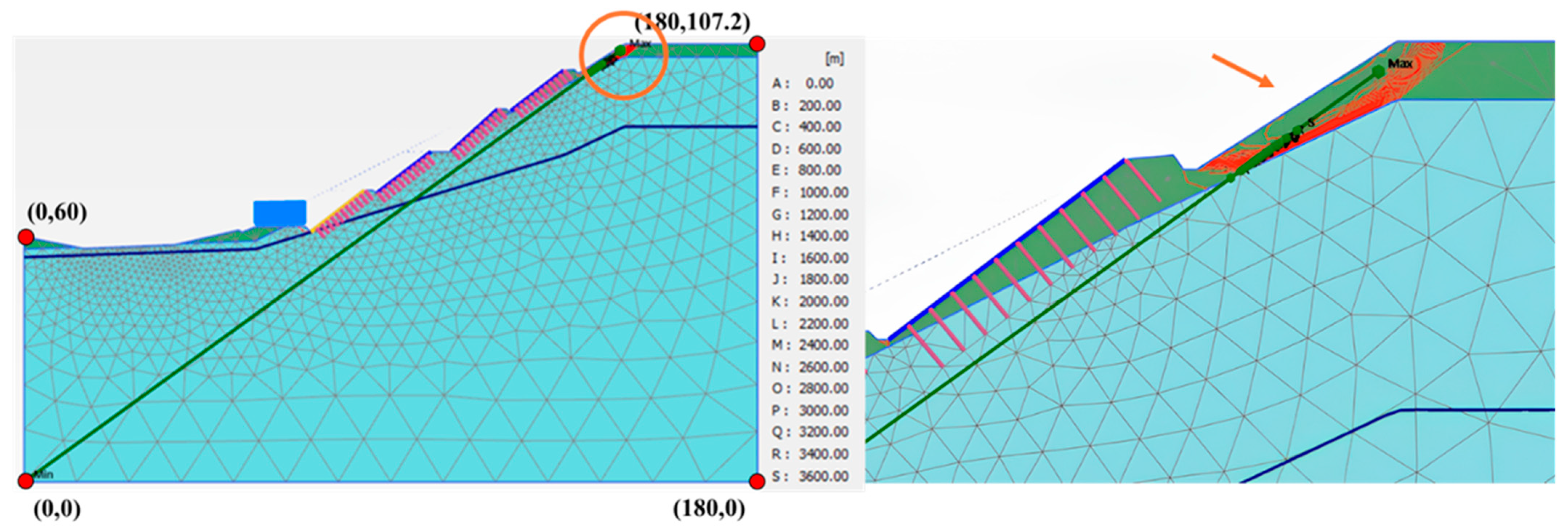
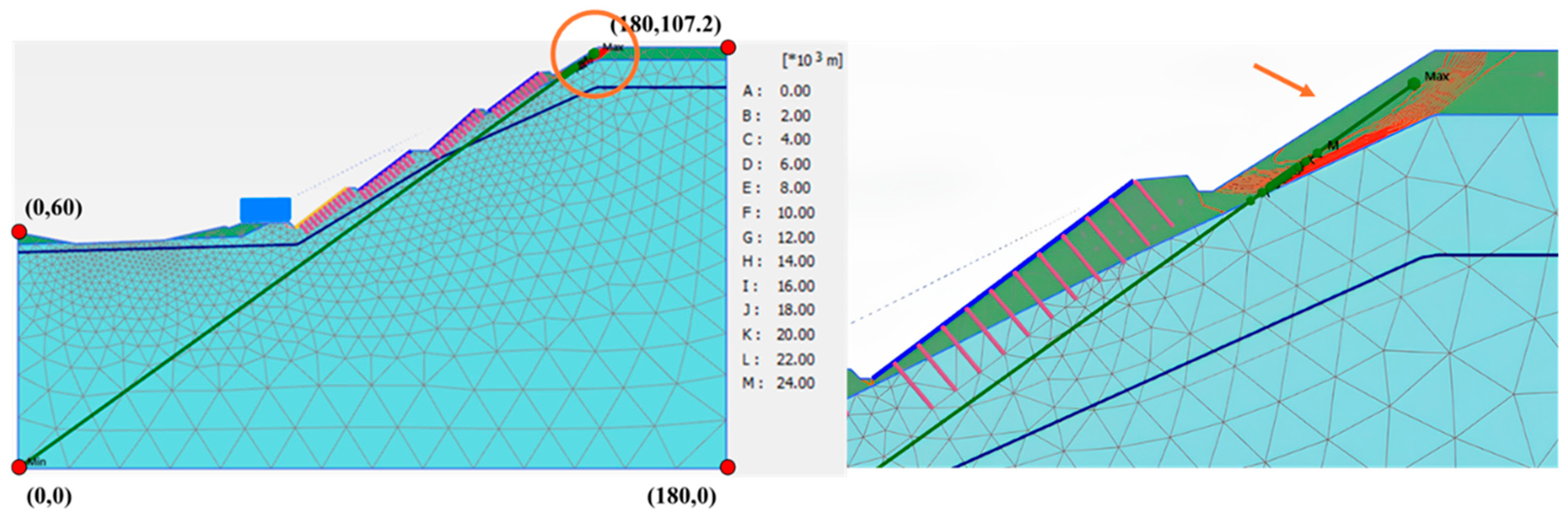
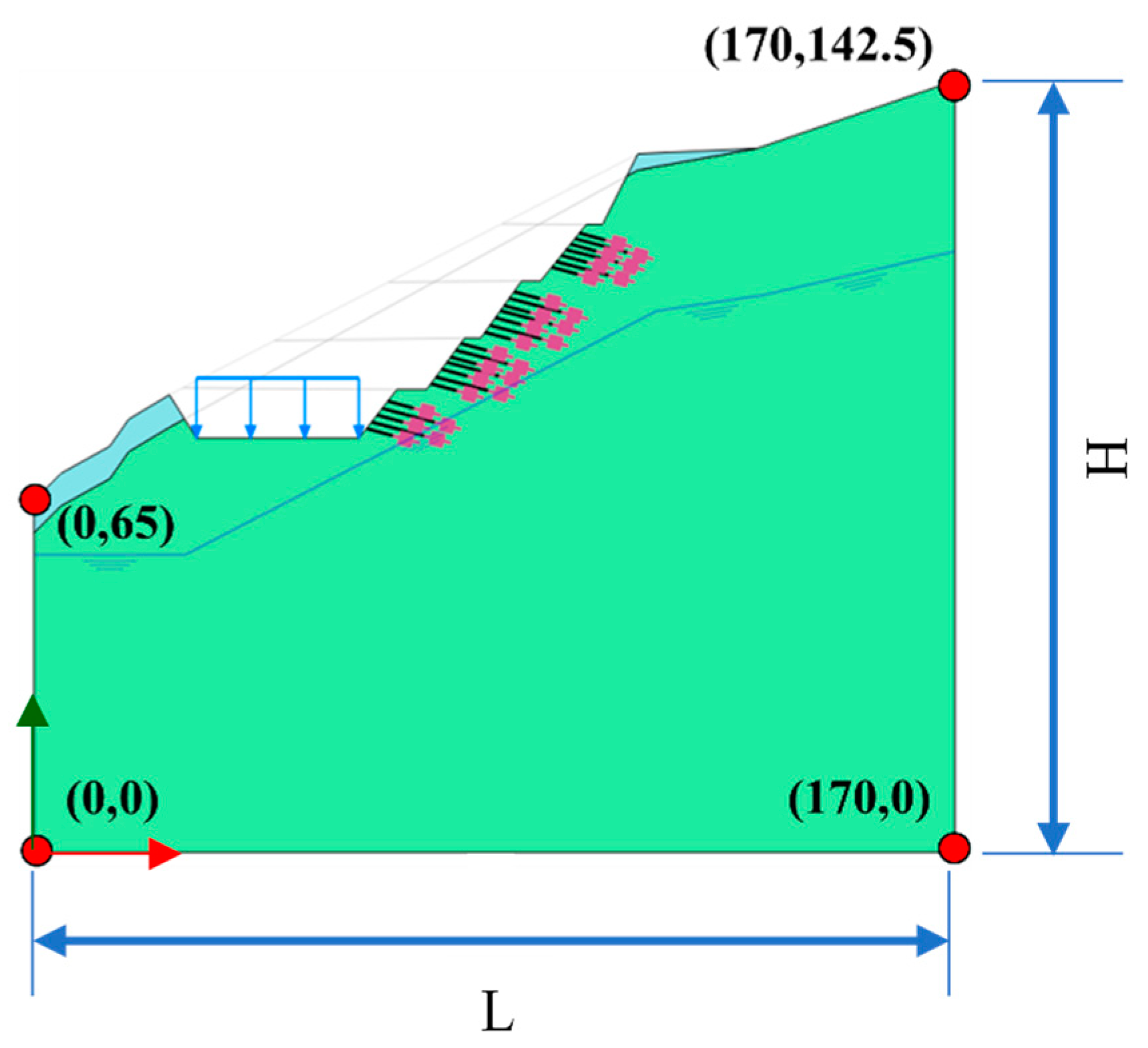
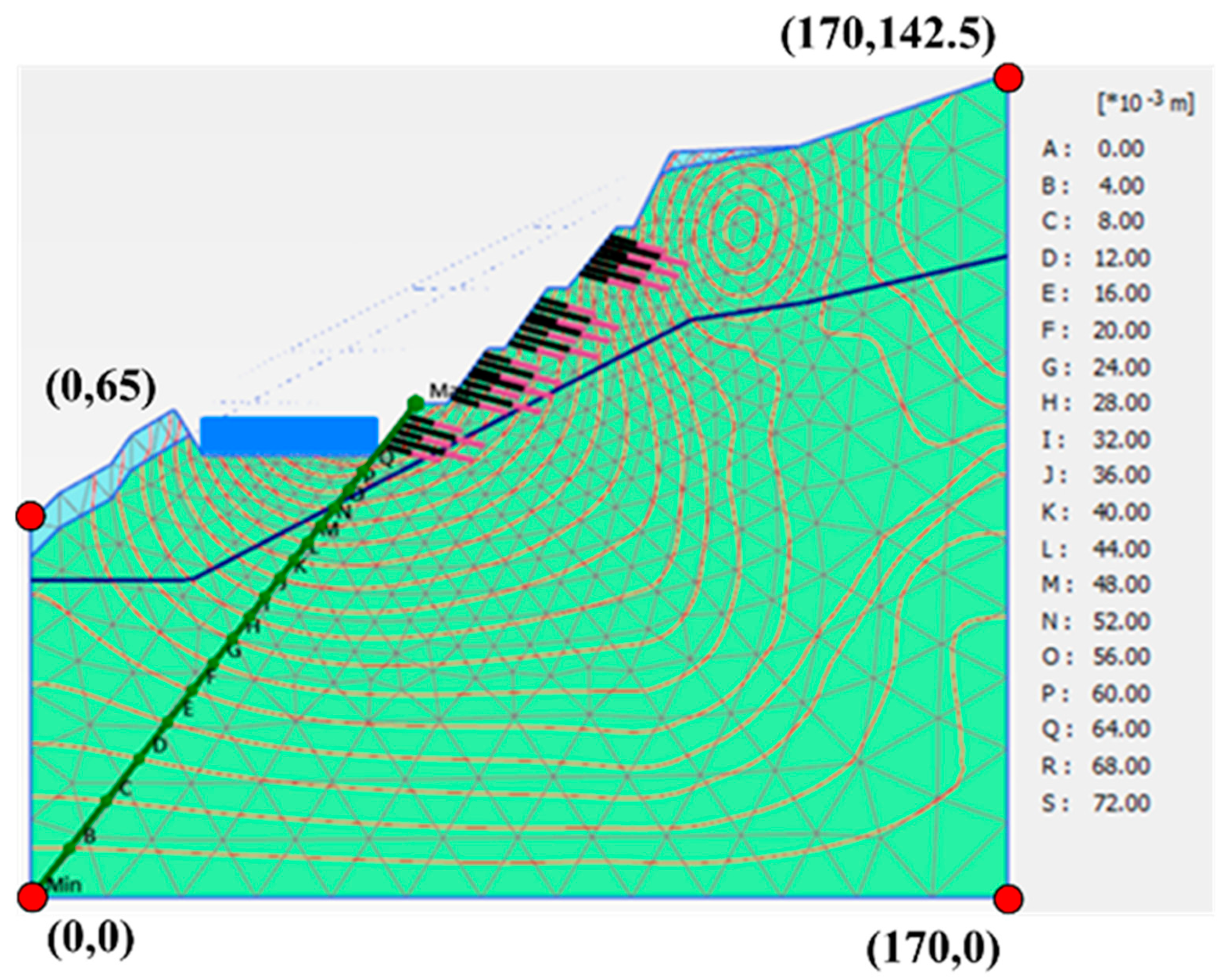
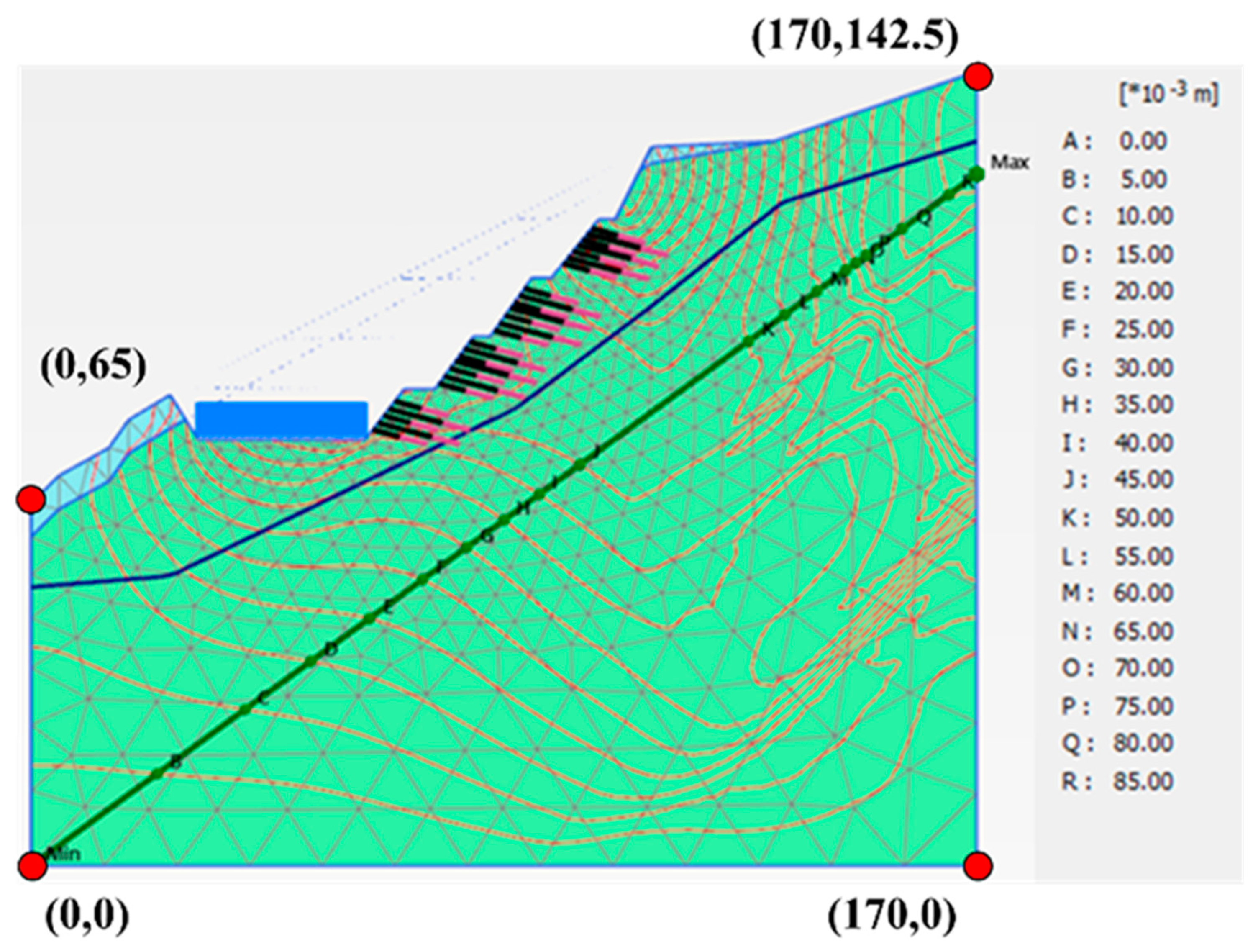
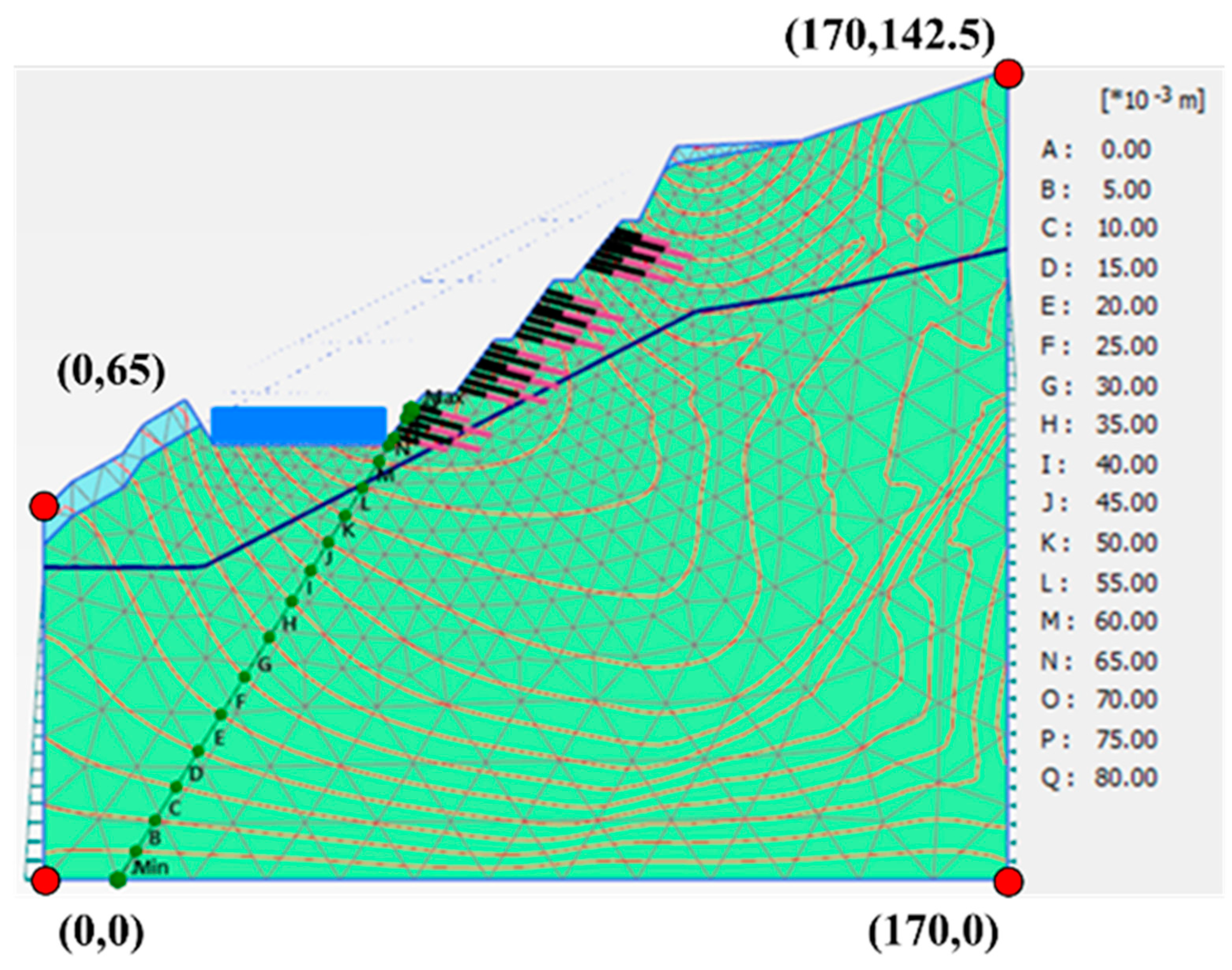
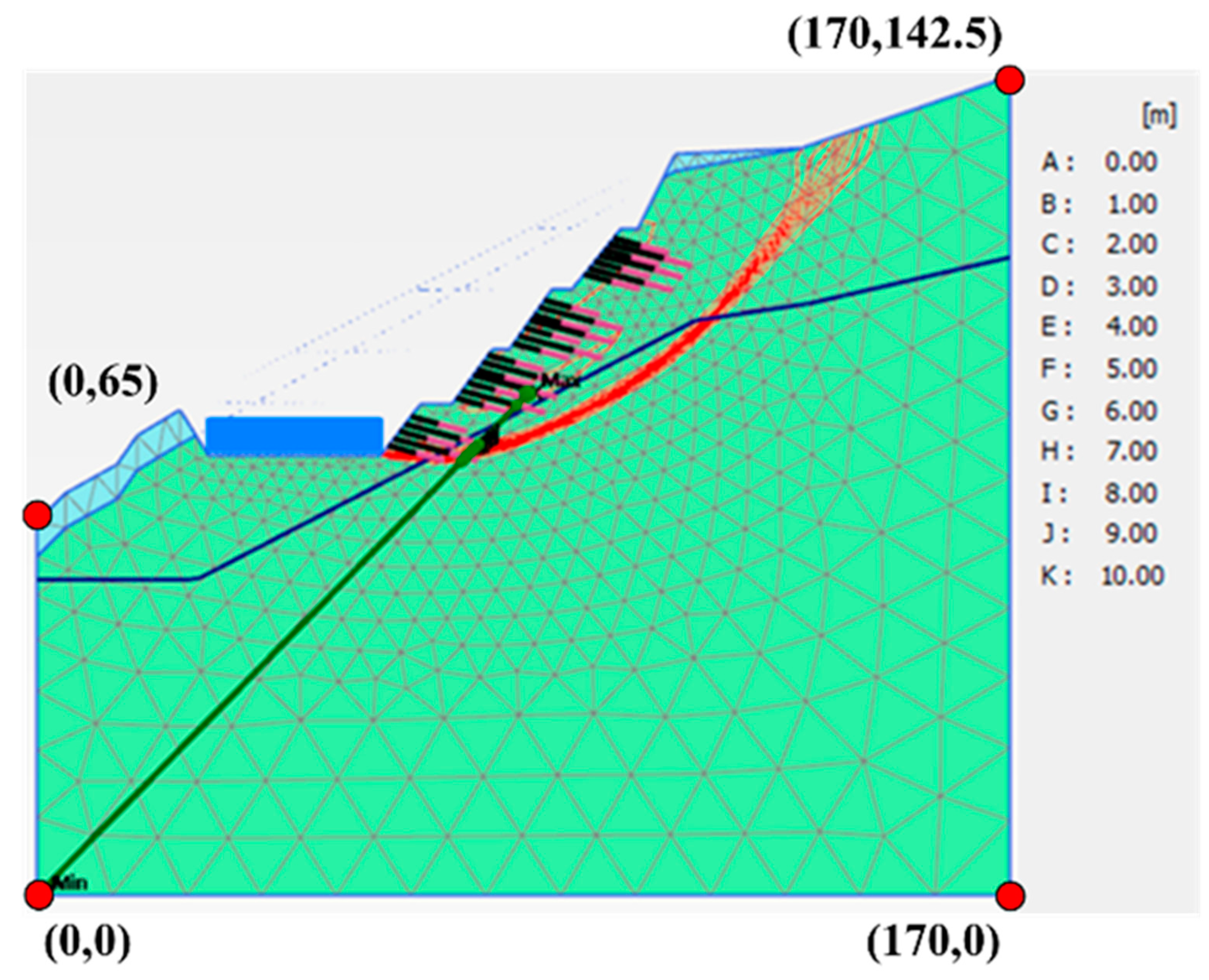
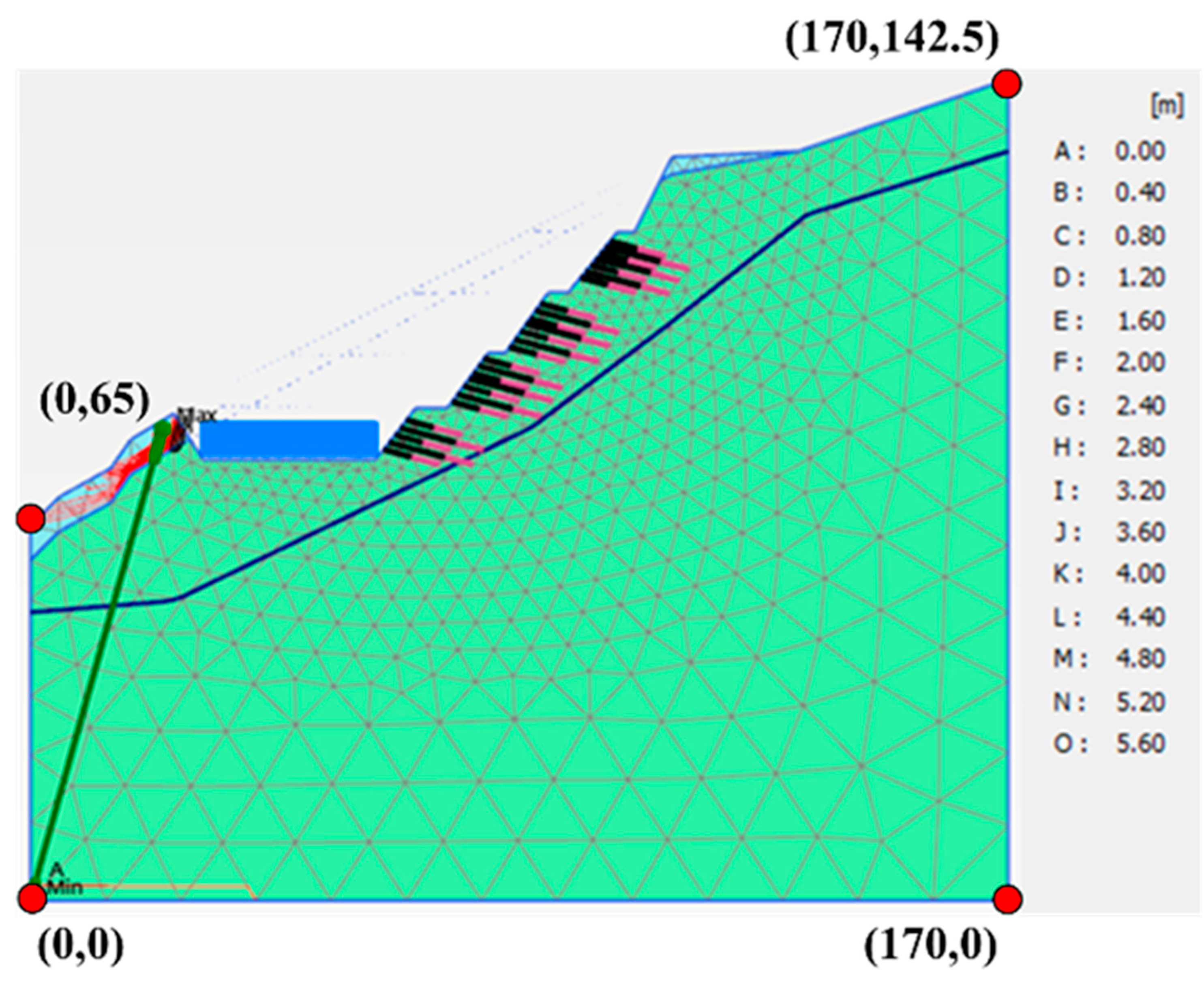
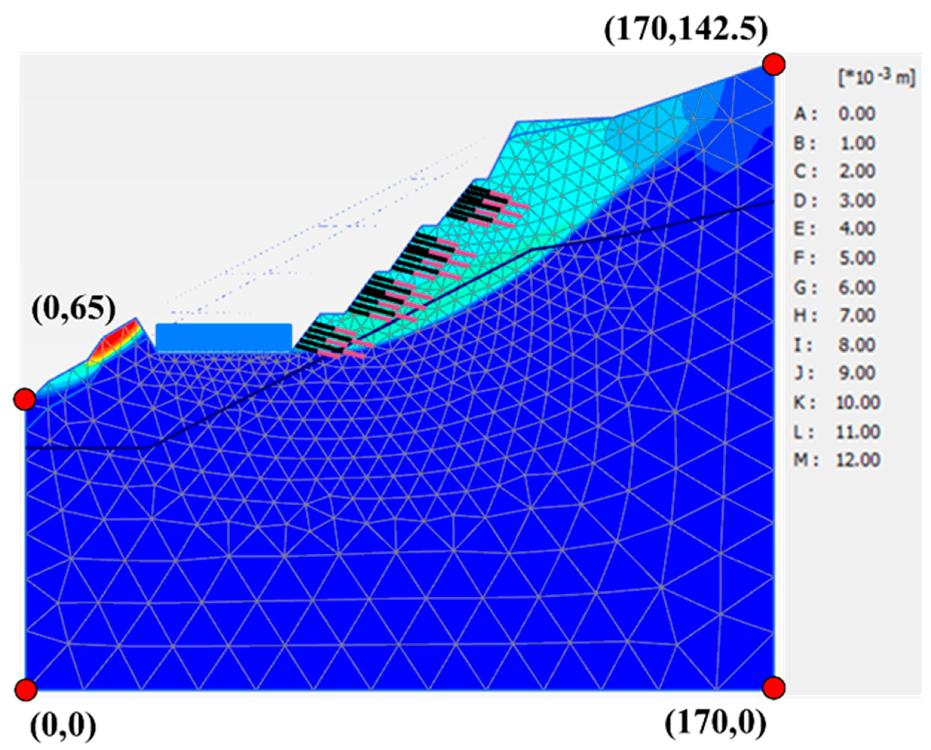
5.3.2. Case Simulation of Site 2
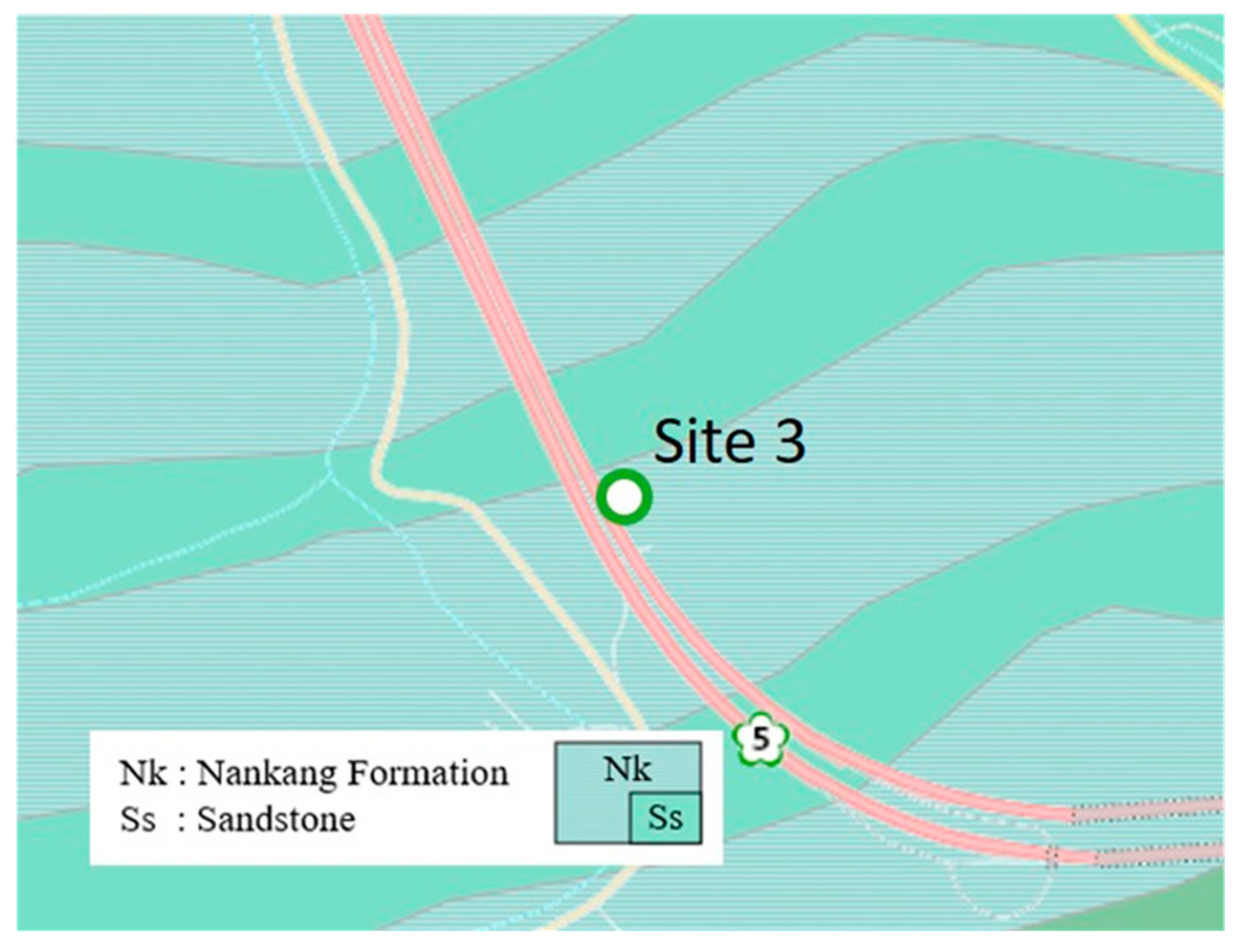
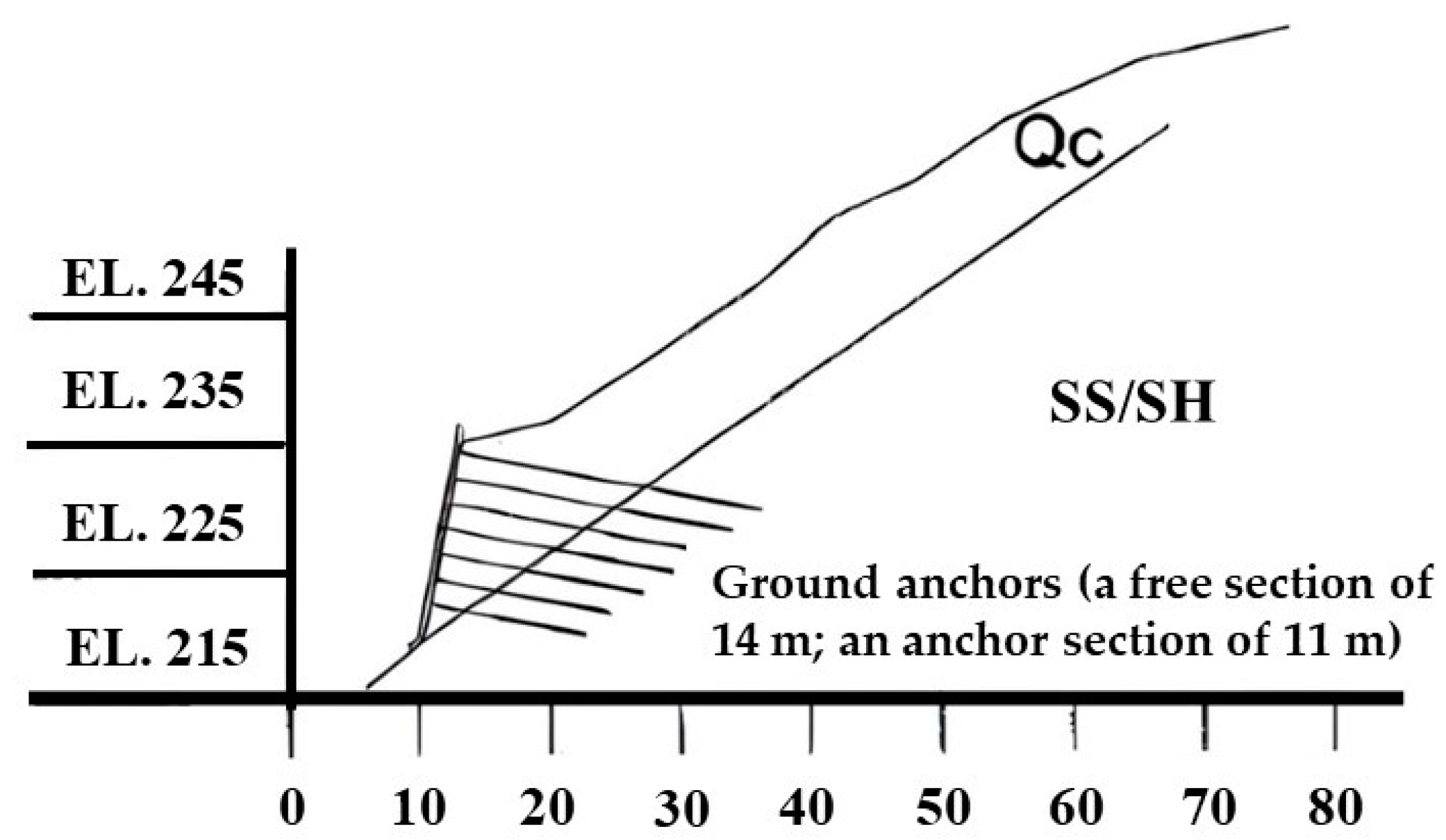
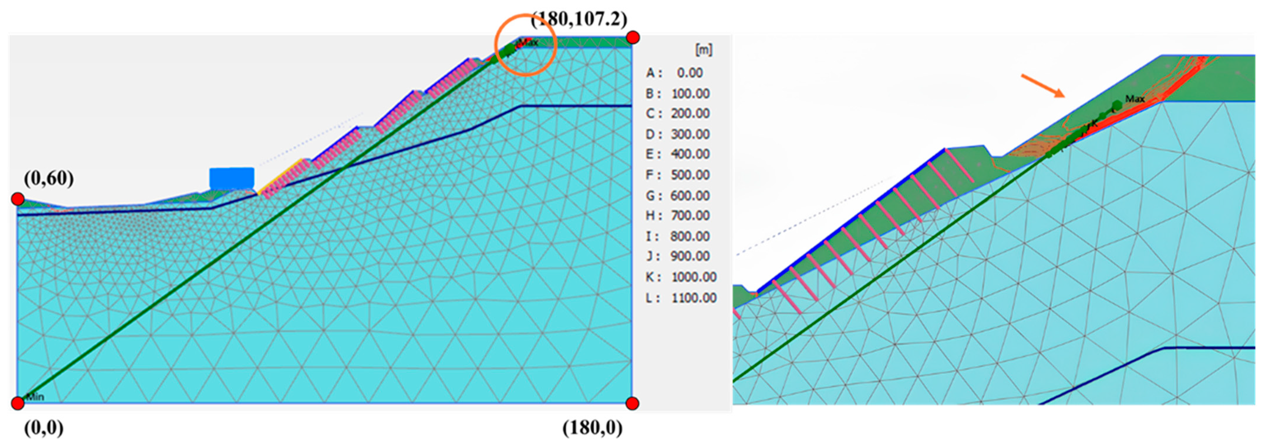
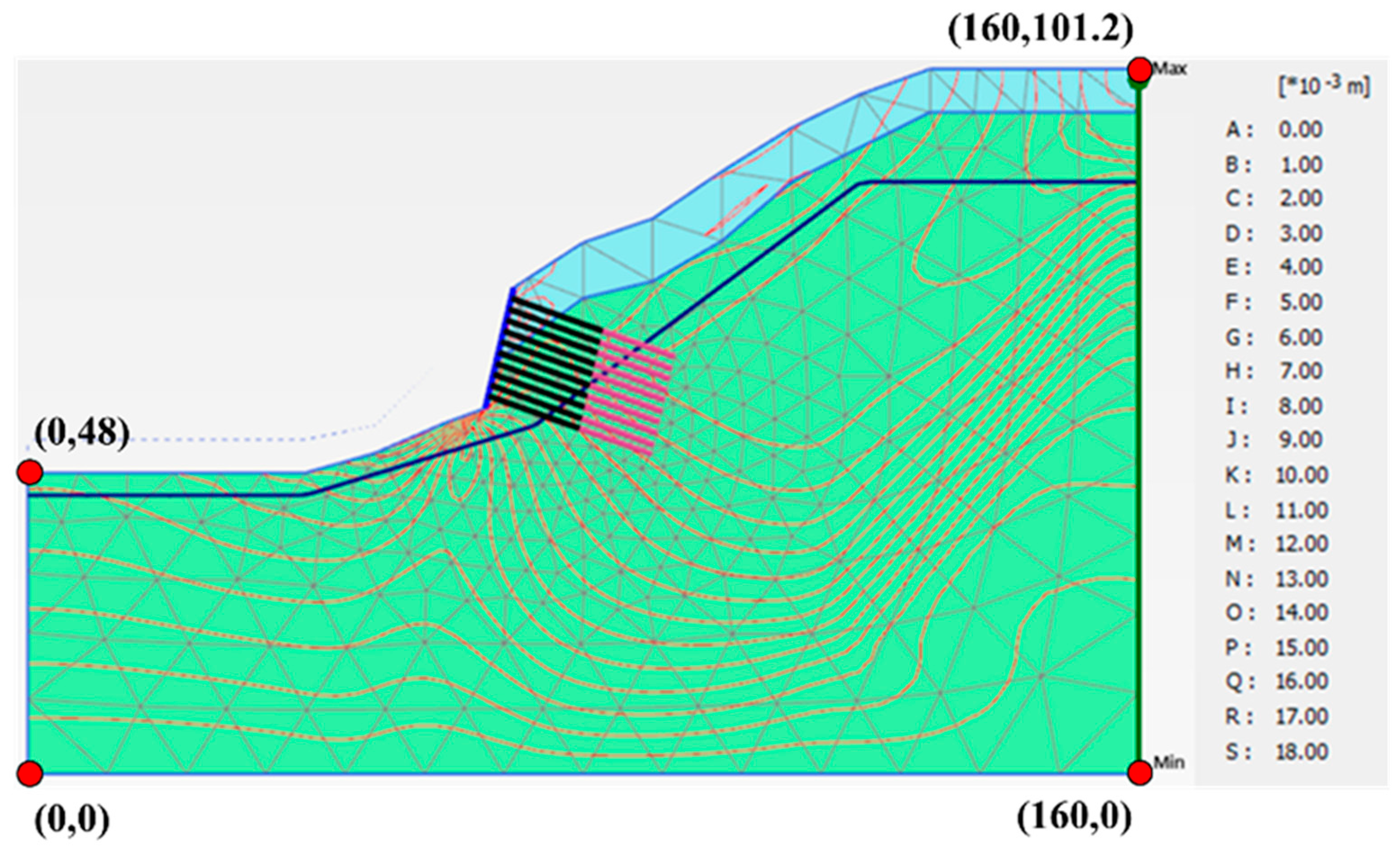
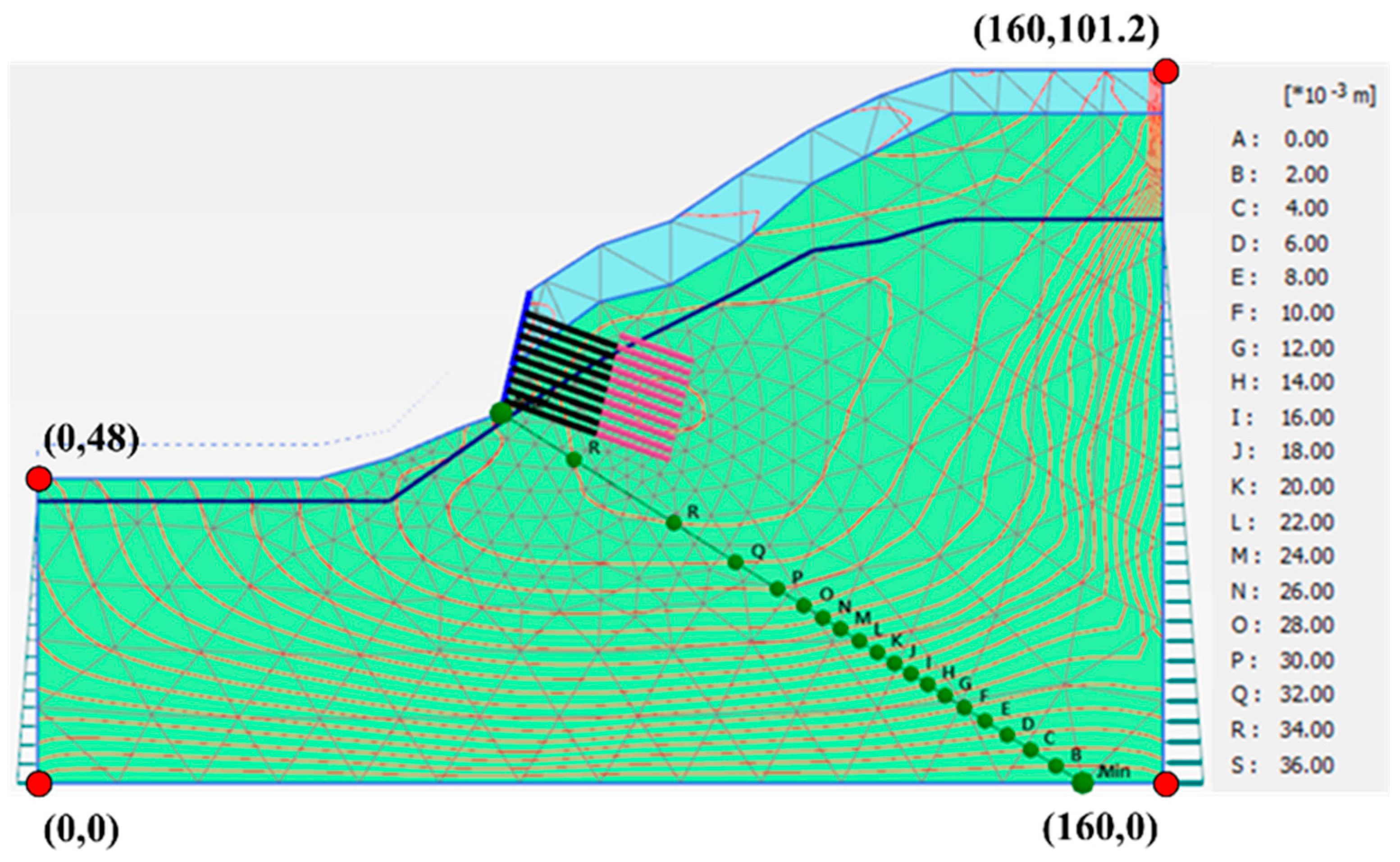
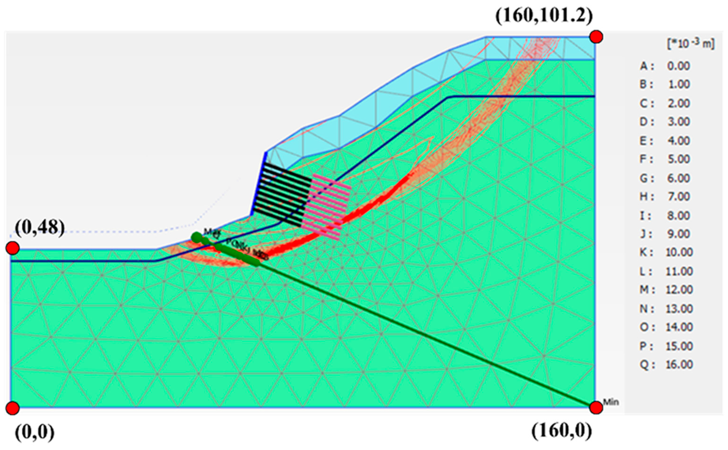
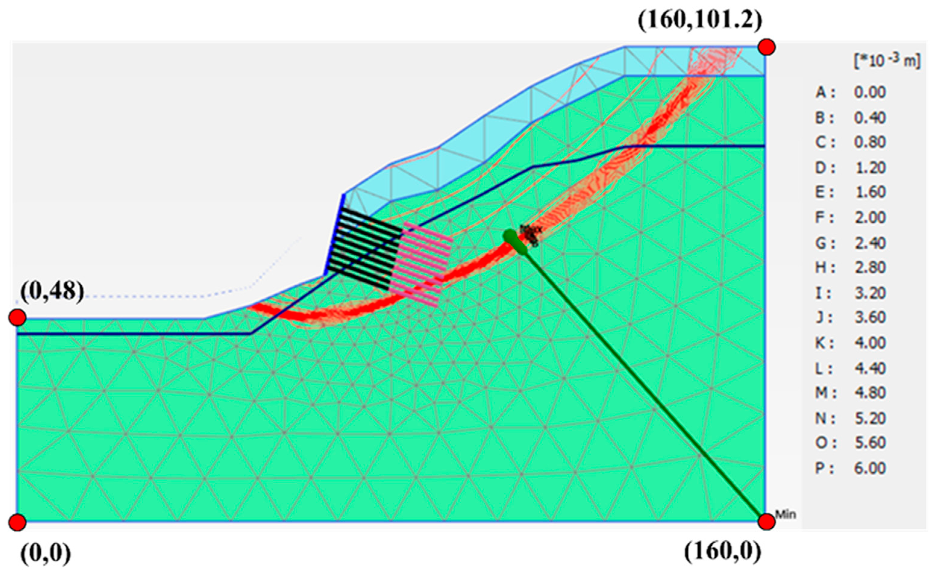
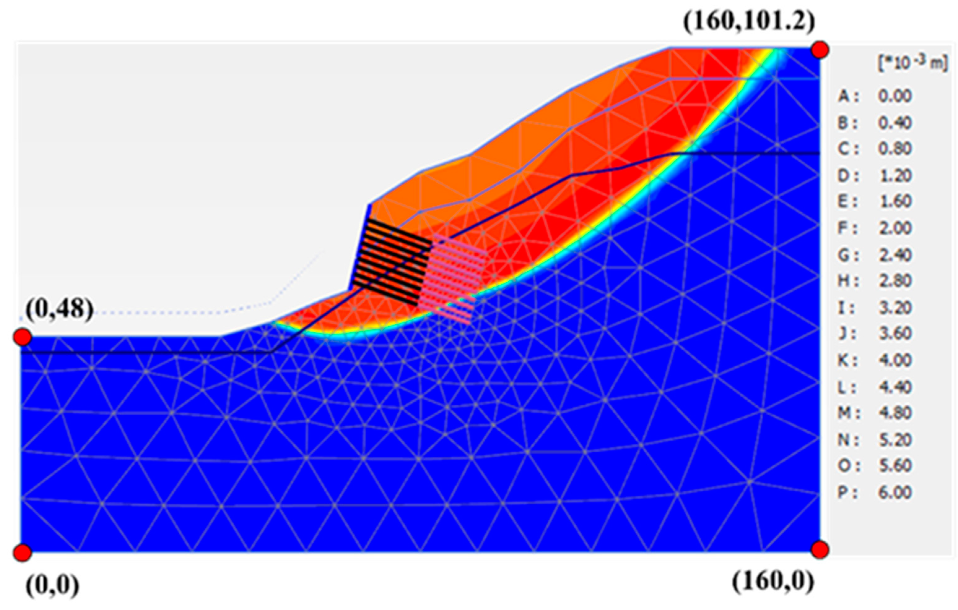
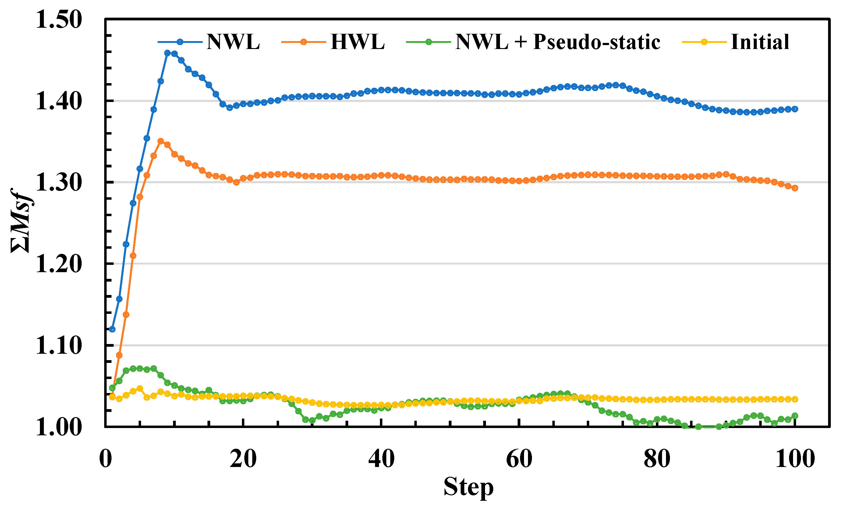
5.3.3. Case Simulation of Site 3
6. Conclusions
- Because the gradients at Sites 1 and 2 were similar, the simulation results showed that, with a normal groundwater level, the force acting on the slope was mostly located at the position of the sliding surface. In the high groundwater level analysis, the force acting on the slope extended to the top.
- Due to the superior strength of the soil, Site 1 saw comparatively little displacement at both normal and high groundwater levels during the analysis.
- The displacement at the top of the slope increased as the groundwater level rose, regardless of whether the slope analysis was conducted with a normal or high groundwater level.
- According to the analysis results, in three different scenarios, the SF value of the slope of Site 1 was greater than the design specification value. This indicates that the slope protection project at Site 1 is working effectively.
- According to the analysis results, the effect of the slope protection project at Sites 2 and 3 needs to be improved.
Author Contributions
Funding
Institutional Review Board Statement
Informed Consent Statement
Data Availability Statement
Conflicts of Interest
References
- Xu, W.J.; Jie, Y.X.; Li, Q.B.; Wang, X.B.; Yu, Y.Z. Genesis, mechanism, and stability of the Dongmiaojia landslide, yellow river, China. Int. J. Rock Mech. Min. Sci. 2014, 67, 57–68. [Google Scholar] [CrossRef]
- Rahman, H.A.; Mapjabil, J. Landslides disaster in Malaysia: An overview. Health 2017, 8, 58–71. [Google Scholar]
- Froude, M.J.; Petley, D.N. Global fatal landslide occurrence from 2004 to 2016. Nat. Hazards Earth Syst. Sci. 2018, 18, 2161–2181. [Google Scholar] [CrossRef]
- Duncan, J.M. State of the art: Limit equilibrium and finite-element analysis of slopes. ASCE J. Geotech. Eng. 1996, 122, 577–596. [Google Scholar] [CrossRef]
- Kardani, N.; Zhou, A.; Nazem, M.; Shen, S.L. Improved prediction of slope stability using a hybrid stacking ensemble method based on finite element analysis and field data. J. Rock Mech. Geotech. Eng. 2021, 13, 188–201. [Google Scholar] [CrossRef]
- Ahmadi, R.; Jahromi, S.G.; Shabakhty, N. Reliability analysis of external and internal stability of reinforced soil under static and seismic loads. Geomech. Eng. 2022, 29, 599–614. [Google Scholar] [CrossRef]
- Chen, S.L.; Tsai, Y.H.; Tang, C.W.; Chu, C.Y.; Chiu, H.W. Case Studies on Numerical Analysis of Slope Stability of National Expressway in Northern Taiwan. In Proceedings of the ACEM22/Structures22, Seoul, Republic of Korea, 16–19 August 2022. [Google Scholar]
- Li, M.; Xiu, Z.; Han, J.; Meng, F.; Wang, F.; Ji, H. Characterization and Stability Analysis of Rock Mass Discontinuities in Layered Slopes: A Case Study from Fushun West Open-Pit Mine. Appl. Sci. 2024, 14, 11330. [Google Scholar] [CrossRef]
- Tang, H.; Wasowski, J.; Juang, C.H. Geohazards in the three Gorges reservoir area, China—Lessons learned from decades of research. Eng. Geol. 2019, 261, 105267. [Google Scholar] [CrossRef]
- Huang, D.; Luo, S.; Zhong, Z. Analysis and modeling of the combined effects of hydrological factors on a reservoir bank slope in the Three Gorges Reservoir area, China. Eng. Geol. 2020, 279, 105858. [Google Scholar] [CrossRef]
- Technical Specifications “Freeway Maintenance Manual”, the National Freeway Bureau, Taiwan District; Ministry of Transportation and Communications: Taipei, Taiwan, 2023. (In Chinese)
- Zhou, J.; Qin, C. Stability analysis of unsaturated soil slopes under reservoir drawdown and rainfall conditions: Steady and transient state analysis. Comput. Geotech. 2022, 142, 104541. [Google Scholar] [CrossRef]
- Hung, J.J. Application of Engineering Geology in Natural Slope Stability (Except Mechanical Factors). J. Geotech. Technol. 1984, 7, 35–42. (In Chinese) [Google Scholar]
- Nie, X.; Chen, K.; Zou, D.; Kong, X.; Liu, J.; Qu, Y. Slope stability analysis based on SBFEM and multistage polytree-based refinement algorithms. Comput. Geotech. 2022, 149, 104861. [Google Scholar] [CrossRef]
- Metya, S.; Chaudhary, N.; Sharma, K.K. Psuedo static stability analysis of rock slope using patton’s shear criterion. Int. J. Geo-Eng. 2021, 12, 7. [Google Scholar] [CrossRef]
- Xu, J.S.; Li, Y.X.; Yang, X.L. Seismic and static 3D stability of two-stage slope considering joined influences of nonlinearity and dilatancy. KSCE J. Civ. Eng. 2018, 22, 3827–3836. [Google Scholar] [CrossRef]
- Pang, H.P.; Nie, X.P.; Sun, Z.B.; Hou, C.Q.; Dias, D.; Wei, B.X. Upper Bound Analysis of 3D-Reinforced Slope Stability Subjected to Pore-Water Pressure. Int. J. Geomech. 2020, 20, 06020002. [Google Scholar] [CrossRef]
- Bishop, A.W. The use of the Slip Circle in the Stability Analysis of Slopes. Géotechnique 1991, 5, 7–17. [Google Scholar] [CrossRef]
- Fredlund, D.G.; Krahn, J. Comparison of slope stability methods of analysis. Can. Geotech. J. 1977, 14, 429–439. [Google Scholar] [CrossRef]
- Zheng, H. A three-dimensional rigorous method for stability analysis of landslides. Eng. Geol. 2012, 145–146, 30–40. [Google Scholar] [CrossRef]
- Kafle, L.; Xu, W.J.; Zeng, S.Y.; Nagel, T. A numerical investigation of slope stability influenced by the combined effects of reservoir water level fluctuations and precipitation: A case study of the Bianjiazhai landslide in China. Eng. Geol. 2022, 297, 106508. [Google Scholar] [CrossRef]
- Kontoe, S.; Summersgill, F.C.; Potts, D.M.; Lee, Y. On the effectiveness of slope stabilising piles for soils with distinct strain-softening behaviour. Géotechnique 2022, 72, 309–321. [Google Scholar] [CrossRef]
- Yang, T.; Rao, Y.; Ma, N.; Feng, J.; Feng, H.; Wang, H. A new method for defining the local factor of safety based on displacement isosurfaces to assess slope stability. Eng. Geol. 2022, 300, 106587. [Google Scholar] [CrossRef]
- Sun, G.; Lin, S.; Zheng, H.; Tan, Y.; Sui, T. The virtual element method strength reduction technique for the stability analysis of stony soil slopes. Comput. Geotech. 2020, 119, 103349. [Google Scholar] [CrossRef]
- Zienkiewicz, O.C.; Humpheson, C.; Lewis, R.W. Associated and Non-Associated Visco-Plasticity and Plasticity in Soil Mechanics. Géotechnique 1975, 25, 671–689. [Google Scholar] [CrossRef]
- Giam, S.K.; Donald, I.B. Determination of Critical Slip Surfaces for Slopes via Stress-Strain Calculations. In Proceedings of the Fifth Australia-New Zealand Conference on Geom, Sydney, Australia, 22–23 August 1988; pp. 461–464. [Google Scholar]
- Ugai, K. A method of calculation of total factor of safety of slopes by elastoplastic FEM. Soils Found. 1989, 29, 190–195. [Google Scholar] [CrossRef]
- Brinkgreve, R.B.J.; Bakker, H.L. Nonlinear finite element analysis of safety factors. Comput. Methods Adv. Geomech. 1991, 7, 1117–1122. [Google Scholar]
- Matsui, T.; San, K.C. Finite Element Slope Stability Analysis by Shear Strength Reduction Technique. Soils Found. 1992, 32, 59–70. [Google Scholar] [CrossRef]
- Ugai, K.; Leshchinsky, D. Three-Dimensional Limit Equilibrium and Finite Element Analysis: A Comparison of Results. Soils Found. 1995, 35, 1–7. [Google Scholar] [CrossRef]
- Griffiths, D.V.; Lane, P.A. Slope Stability Analysis by Finite Elements. Géotechnique 1999, 49, 387–403. [Google Scholar] [CrossRef]
- Okabe, S. General theory of earth pressure. J. Jpn. Soc. Civ. Eng. 1924, 6, 1277–1323. [Google Scholar]
- Mononobe, N.; Matsuo, M. On the Determination of Earth Pressures during Earthquakes. In Proceedings of the World Engineering Congress, Tokyo, Japan, 22–28 October 1929; Volume 9, pp. 179–187. [Google Scholar]
- Geological Data Integrated Query System, Geological Survey and Mining Management Center, Ministry of Economic Affairs, Taiwan. Available online: https://geomap.gsmma.gov.tw/gwh/gsb97-1/sys8a/t3/index1.cfm (accessed on 1 January 2021).
- Safety Assessment Report on Four Slopes from National Freeway No. 1, 5.7 Kilometers to Wuda South, Taiwan District Freeway Bureau, Ministry of Transportation and Communications; T.Y.Lin Taiwan Consulting Engineers Inc.: Taipei, Taiwan, 2021. (In Chinese)
- Project Information on Slope Monitoring and Inspection Commissioned Technical Service Work for the Neihu Section and Toucheng Section in 2020 by the North District Maintenance Engineering Bureau of the Freeway Bureau of the Ministry of Transportation and Communications; Hongyi Engineering Consulting Co., Ltd.: Taipei, Taiwan, 2021. (In Chinese)
- Robert, D.J. A Modified Mohr-Coulomb Model to Simulate the Behavior of Pipelines in Unsaturated Soils. Comput. Geotech. 2017, 91, 146–160. [Google Scholar] [CrossRef]
- Labuz, J.F.; Zang, A. Mohr–Coulomb Failure Criterion. Rock Mech. Rock Eng. 2012, 45, 975–979. [Google Scholar] [CrossRef]
- Plaxis 2D, 2D-2-Reference; Connect Edition V2024.2; Bentley: Harrisburg, PA, USA, 2024.
- Code for Seismic Design of Highway Bridges; Ministry of Transportation and Communications: Taipei, Taiwan, 2019. (In Chinese)
- Technical Specifications “Freeway Slope Engineering Design Specifications l”; Ministry of Transportation and Communications: Taipei, Taiwan, 2015. (In Chinese)
- Das, B.M. Principles of Foundation Engineering, 6th ed.; Thomson Canada, Ltd.: Toronto, ON, Canada, 2007; p. 445. [Google Scholar]
- Yang, T.; Zhou, D.P.; Ma, H.M.; Zhang, Z.P. Point safety factor method for stability analysis of landslide. Rock Soil Mech. 2010, 31, 971–975. (In Chinese) [Google Scholar]
- Stead, D.; Wolter, A. A critical review of rock slope failure mechanisms: The importance of structural geology. J. Struct. Geol. 2015, 74, 1–23. [Google Scholar] [CrossRef]
- Rabi, M. Performance of hybrid MSE/soil nail walls using numerical analysis and limit equilibrium approaches. HBRC J. 2016, 12, 63–70. [Google Scholar] [CrossRef]
- Bowles, J.E. Physical and Geotechnical Properties of Soils, 2nd ed.; McGraw-Hill Book Company: New York, NY, USA, 1989; p. 576. [Google Scholar]


| Drilling Code | Depth (m) | Moisture Content (%) | Unit Weight (t/m3) | Compression Strength (MPa) | Strain (%) | Lithology |
|---|---|---|---|---|---|---|
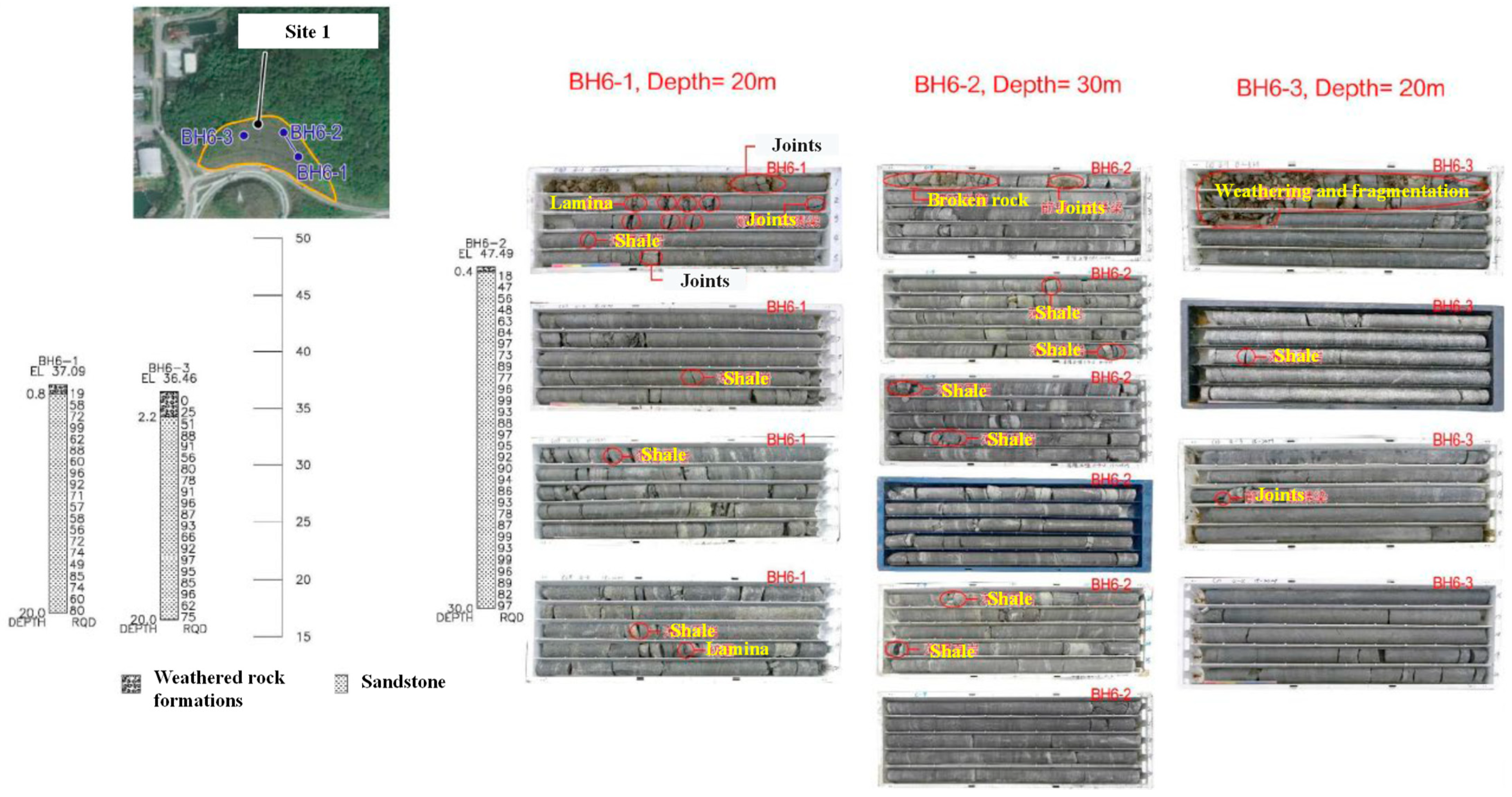
| BH6-1 | 11.1 | 2.6 | 2.63 | 30.9 | 1.44 | Sandstone |
| BH6-2 | 23.1 | 2.5 | 2.60 | 28.4 | 1.38 | Sandstone |
| BH6-3 | 3.1 | 3.1 | 2.61 | 17.2 | 1.59 | Sandstone |
| Drilling Code | Depth (m) | Moisture Content (%) | Peak Strength | Residual Strength | Lithology | ||
|---|---|---|---|---|---|---|---|
| cp (MPa) | φp (°) | cr (MPa) | φr (°) | ||||
| BH6-1 | 3–4 | 3.3–5.5 | 0.70 | 29.6 | 0.34 | 28.8 | Sandstone |
| BH6-2 | 12–13 | 2.5–6.5 | 9.09 | 53.8 | 1.26 | 44.2 | Sandstone |
| BH6-3 | 4–5 | 5–9.3 | 2.50 | 44.6 | 1.21 | 37.5 | Sandstone |
| Site Code | Point A | Point B | Point C | Point D | L (m) | H (m) |
|---|---|---|---|---|---|---|
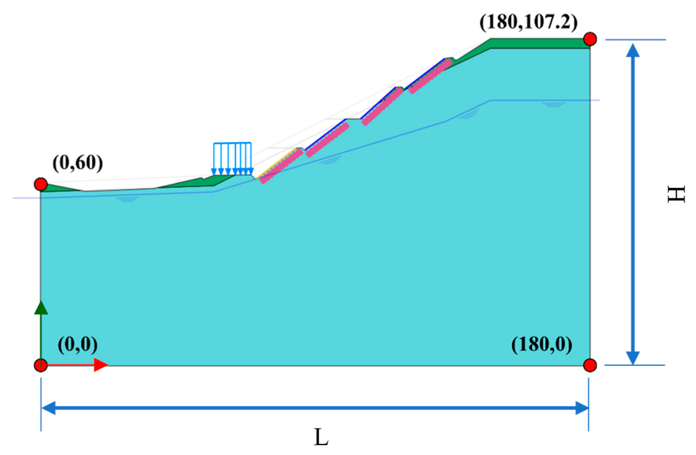
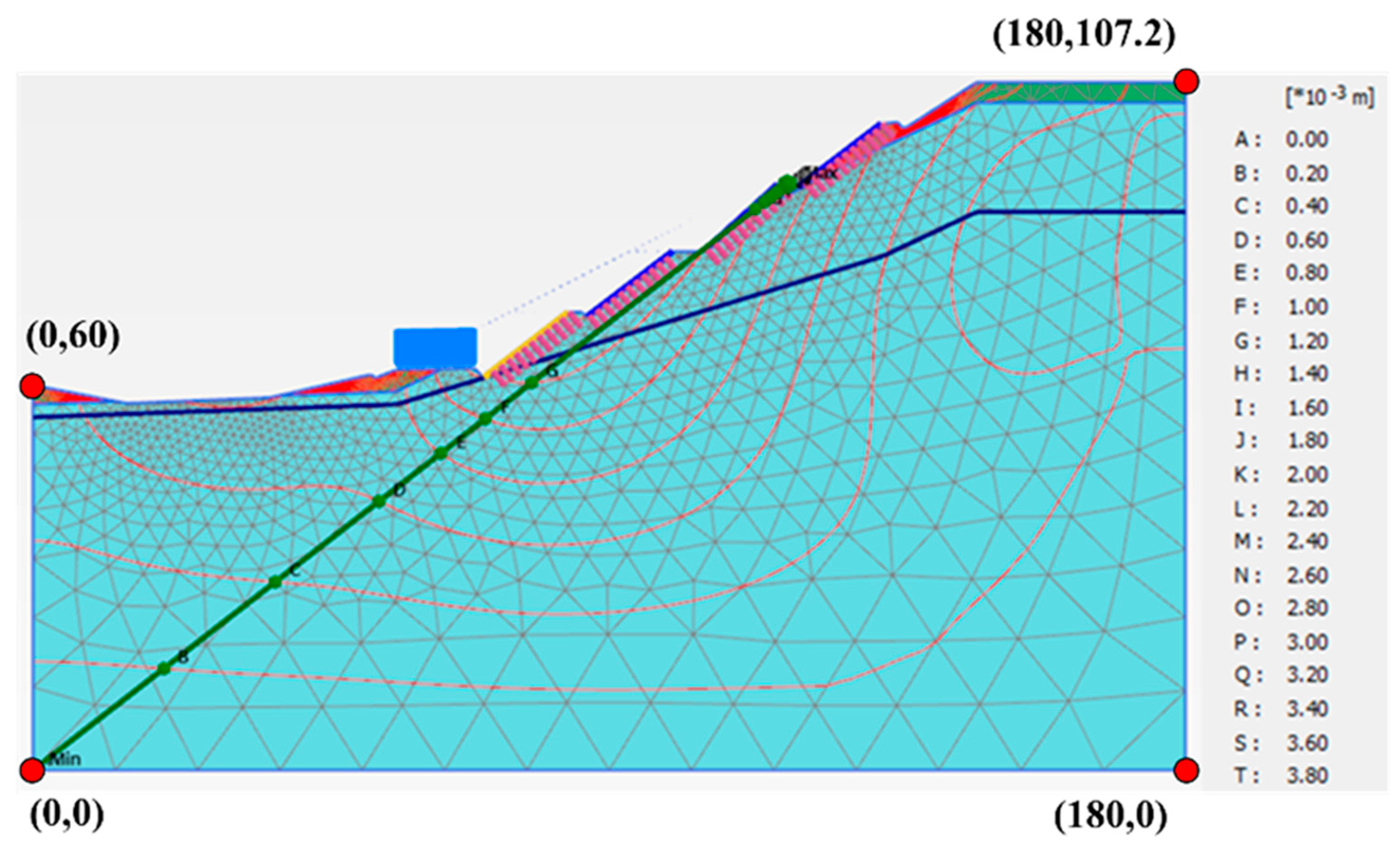
| Site 1 | (0, 0) | (0, 60) | (180, 107.2) | (180, 0) | 180 | 107.2 |
| Site 2 | (0, 0) | (0, 65) | (170, 142.5) | (170, 0) | 170 | 142.5 |
| Site 3 | (0, 0) | (0, 48) | (160, 101.2) | (160, 0) | 160 | 101.2 |
| Soil Layer | Parameters | ||||||
|---|---|---|---|---|---|---|---|
(kN/m3) | (kN/m3) | E (kN/m2) | ν | c (kN/m2) | φ (°) | ψ (°) | |
| Weathered rock layer | 22.0 | 22.5 | 2.5 × 10⁴ | 0.25 | 10 | 28 | 0 |
| Sandstone layer | 25.2 | 25.7 | 4 × 10⁶ | 0.25 | 150 | 26 | 0 |
| Simulation Elements | Young’s Modulus (kN/m2) | Unit Weight (kN/m3) | Diameter (cm) | Horizontal Spacing (m) | Front End Side Friction Resistance (kN/m) | Rear End Side Friction Resistance (kN/m) |
|---|---|---|---|---|---|---|
| Embedded beam row element | 2.5 × 10⁷ | 10 | 25 | 3 | 509 | 509 |
| Simulation Elements | Material Type | Axial Stiffness (kN/m) | Flexural Stiffness (kNm2/m) | Weight (kN/m/m) | ν |
|---|---|---|---|---|---|
| Plate element | Elasticity | 7.53 × 10⁶ | 7.06 | 0.17 |
| scenarios | |u| (mm) | (mm) | (mm) | ||
|---|---|---|---|---|---|
| Max | Min | Max | Min | ||
| Normal groundwater level | 3.86 | 1.62 | −0.30 | 3.56 | −0.50 |
| High groundwater level | 3.26 | 1.69 | −0.47 | 2.82 | −1.13 |
| Normal groundwater level and pseudo-static analysis | 24.10 | 0 | −20.54 | 2.46 | −13.53 |
| Safety Factor | Slope Condition | Meaning |
|---|---|---|
| SF < 1.07 | Frequent occurrence of slope collapse | Labile |
| 1.07 < SF < 1.25 | Slope collapse sometimes occurs | Critical |
| SF > 1.25 | Slope collapse events are rare | Stable |
| Scenarios | Safety Factor | |
|---|---|---|
| Simulation Result | Design Specification | |
| Scenario 1: normal groundwater level | 1.627 | ≧1.5 |
| Scenario 2: high groundwater level | 1.626 | ≧1.2 |
| Scenario 3: normal groundwater level and pseudo-static analysis | 1.223 | ≧1.1 |
| Soil Layer | Parameters | ||||||
|---|---|---|---|---|---|---|---|
(kN/m3) | (kN/m3) | E (kN/m2) | ν | c (kN/m2) | φ (°) | ψ (°) | |
| Colluvium | 19.6 | 20.1 | 7 × 10⁴ | 0.3 | 10 | 28 | 0 |
| Weathered sandstone | 23.5 | 24.0 | 3 × 10⁵ | 0.3 | 50 | 30 | 0 |
| Simulation Elements | Young’s Modulus (kN/m2) | Unit Weight (kN/m3) | Diameter (cm) | Horizontal Spacing (m) | Front End Side Friction Resistance (kN/m) | Rear End Side Friction Resistance (kN/m) |
|---|---|---|---|---|---|---|
| Embedded beam row element | 2.5 × 10⁷ | 10 | 20 | 3 | 95.5 | 95.5 |
| Simulation Elements | Material Type | Axial Stiffness (kN/m) | Horizontal Spacing (m) | Pre-Force (kN/m) |
|---|---|---|---|---|
| Node-to-node anchor element | Elasticity | 2 × 10⁵ | 3 | 300 |
| scenario | |u| (mm) | (mm) | (mm) | ||
|---|---|---|---|---|---|
| Max | Min | Max | Min | ||
| Normal groundwater level | 75.12 | 17.51 | −29.20 | 73.30 | −30.05 |
| High groundwater level | 89.16 | 14.88 | −47.95 | 56.64 | −89.16 |
| Normal groundwater level and pseudo-static analysis | 80.32 | 0 | −58.59 | 64.86 | −47.62 |
| Scenarios | Safety Factor | |
|---|---|---|
| Simulation Result | Design Specification | |
| Scenario 1: Normal groundwater level | 1.265 | ≧1.5 |
| Scenario 2: High groundwater level | 1.105 | ≧1.2 |
| Scenario 3: Normal groundwater level and pseudo-static analysis | 1.009 | ≧1.1 |
| Soil Layer | Parameters | ||||||
|---|---|---|---|---|---|---|---|
(kN/m3) | (kN/m3) | E (kN/m2) | ν | c (kN/m2) | φ (°) | ψ (°) | |
| Colluvial layer | 18.6 | 19.1 | 7 × 10⁴ | 0.3 | 10 | 28 | 0 |
| Interbedded sandstone and shale | 25.5 | 26.0 | 3 × 10⁵ | 0.3 | 50 | 35 | 5 |
| Simulation Elements | Material Type | Axial Stiffness (kN/m) | Flexural Stiffness (kNm2/m) | Weight (kN/m/m) | ν |
|---|---|---|---|---|---|
| Plate element | Elasticity | 7.53 × 10⁶ | 7.2 | 0.17 |
| Simulation Elements | Young’s Modulus (kN/m2) | Unit Weight (kN/m3) | Diameter (cm) | Horizontal Spacing (m) | Front End Side Friction Resistance (kN/m) | Rear End Side Friction Resistance (kN/m) |
|---|---|---|---|---|---|---|
| Embedded beam row element | 2.5 × 10⁷ | 10 | 20 | 2.5 | 86.8 | 86.8 |
| Simulation Elements | Material Type | Axial Stiffness (kN/m) | Horizontal Spacing (m) | Pre-Force (kN/m) |
|---|---|---|---|---|
| Node-to-node anchor element | Elasticity | 2 × 10⁵ | 2.5 | 600 |
| scenario | |u| (mm) | (mm) | |||
|---|---|---|---|---|---|
| Max | Min | Max | Min | ||
| Normal groundwater level | 16.41 | 2.70 | −6.22 | 6.31 | −3.80 |
| High groundwater level | 18.74 | 1.99 | −12.83 | 4.19 | −18.74 |
| Normal groundwater level and pseudo-static analysis | 37.45 | 0 | −36.83 | 9.15 | −25.42 |
| Scenarios | Safety Factor | |
|---|---|---|
| Simulation Result | Design Specification | |
| Scenario 1: Normal groundwater level | 1.405 | ≧1.5 |
| Scenario 2: High groundwater level | 1.306 | ≧1.2 |
| Scenario 3: Normal groundwater level and pseudo-static analysis | 1.021 | ≧1.1 |
Disclaimer/Publisher’s Note: The statements, opinions and data contained in all publications are solely those of the individual author(s) and contributor(s) and not of MDPI and/or the editor(s). MDPI and/or the editor(s) disclaim responsibility for any injury to people or property resulting from any ideas, methods, instructions or products referred to in the content. |
© 2025 by the authors. Licensee MDPI, Basel, Switzerland. This article is an open access article distributed under the terms and conditions of the Creative Commons Attribution (CC BY) license (https://creativecommons.org/licenses/by/4.0/).
Share and Cite
Chiu, H.-W.; Tsai, Y.-H.; Tang, C.-W.; Chu, C.-Y.; Chen, S.-L. A Case Study of Using Numerical Analysis to Assess the Slope Stability of National Freeways in Northern Taiwan. Appl. Sci. 2025, 15, 635. https://doi.org/10.3390/app15020635
Chiu H-W, Tsai Y-H, Tang C-W, Chu C-Y, Chen S-L. A Case Study of Using Numerical Analysis to Assess the Slope Stability of National Freeways in Northern Taiwan. Applied Sciences. 2025; 15(2):635. https://doi.org/10.3390/app15020635
Chicago/Turabian StyleChiu, Hao-Wei, Yi-Hao Tsai, Chao-Wei Tang, Chih-Yu Chu, and Shong-Loong Chen. 2025. "A Case Study of Using Numerical Analysis to Assess the Slope Stability of National Freeways in Northern Taiwan" Applied Sciences 15, no. 2: 635. https://doi.org/10.3390/app15020635
APA StyleChiu, H.-W., Tsai, Y.-H., Tang, C.-W., Chu, C.-Y., & Chen, S.-L. (2025). A Case Study of Using Numerical Analysis to Assess the Slope Stability of National Freeways in Northern Taiwan. Applied Sciences, 15(2), 635. https://doi.org/10.3390/app15020635