Abstract
The lunar calendar is often overlooked in time-series data modeling despite its importance in understanding seasonal patterns, as well as economics, natural phenomena, and consumer behavior. This study aimed to investigate the effectiveness of the lunar calendar in modeling and forecasting rainfall levels using various machine learning methods. The methods employed included long short-term memory (LSTM) and gated recurrent unit (GRU) models to test the accuracy of rainfall forecasts based on the lunar calendar compared to those based on the Gregorian calendar. The results indicated that machine learning models incorporating the lunar calendar generally provided greater accuracy in forecasting for periods of 3, 4, 6, and 12 months compared to models using the Gregorian calendar. The lunar calendar model demonstrated higher accuracy in its prediction, exhibiting smaller errors (MAPE and MBE values), whereas the Gregorian calendar model yielded somewhat larger errors and tended to underestimate the values. These findings contributed to the advancement of forecasting techniques, machine learning, and the adaptation to non-Gregorian calendar systems while also opening new opportunities for further research into lunar calendar applications across various domains.
1. Introduction
The forecasting of time-series data, particularly on a monthly scale, is integral to various sectors, including agriculture, disaster management, and environmental planning. Adjustments to the number of days in a month, whether in the Gregorian or lunar calendar, can influence the accuracy of forecast results [1,2]. Therefore, using the appropriate calendar system for forecasting can lead to more accurate seasonal projections and monthly trends [3]. Additionally, precise monthly forecasting is essential for planning and decision-making, such as disaster mitigation in cases of extreme rainfall [4]. In agriculture, accurate forecasts are especially valuable for the early planning of planting seasons [5,6,7]. In the environmental field, accurate rainfall forecasting is necessary to anticipate disasters such as floods and landslides [8].
Rainfall significantly impacts construction projects by causing delays, increasing safety risks, and affecting material integrity [9,10,11,12]. Accurate rainfall forecasting is necessary for effective project planning and risk management in construction. By predicting rainfall more accurately, construction managers can adjust schedules to avoid delays and allocate resources effectively. This not only ensures the safety of workers but also helps maintain the integrity of materials used in construction. Thus, integrating accurate rainfall forecasts into construction planning is crucial for minimizing disruptions and costs.
Artificial intelligence in virtual design and construction (VDC) enhances these forecasts, allowing for better scheduling and resource allocation [13,14]. The present status of AI in VDC shows promising improvements in predictive modeling and real-time data integration. These advancements enable construction managers to make informed decisions based on accurate weather predictions. Future challenges include further refining these models for greater accuracy and expanding their applications to anticipate and mitigate weather-related disruption in construction [14]. By addressing these challenges, the construction industry can better prepare for and respond to the impacts of rainfall, ensuring safer and more efficient project execution.
In rainfall forecasting, Gregorian and Lunar calendars are two of the world’s most widely used calendar systems, offering distinct advantages and challenges for time-series analysis. Both have an impact on the analysis and prediction of time-series data [15]. The Gregorian calendar, based on the solar cycle, enables consistent scheduling, particularly in the context of international business [16]. In contrast, the lunar calendar, which follows the lunar cycle, is commonly used to plan religious events in Asian and Middle Eastern countries [17,18]. These differences between calendar systems can impact how we forecast seasonal phenomena, such as rainfall or consumption patterns [19].
While both calendar systems provide frameworks for structuring time, their impact on forecasting methodologies varies significantly. The Gregorian calendar’s fixed solar cycle aligns with statistical tools and international standards, making it the default choice for most predictive models [20,21]. However, this alignment can overlook certain seasonal cycles that follow lunar patterns, which are particularly relevant in regions where agricultural or climatic phenomena depend on the lunar calendar. Integrating these unique temporal patterns into forecasting models can yield deeper insights, especially for predicting rainfall and other periodic events. This highlights the importance of tailoring forecasting approaches to the calendar system that is best suited to the natural cycles under study.
The Gregorian calendar is commonly used to model and forecast rainfall levels in various countries. It serves as the basis for modeling time-series data in several statistical models [22,23]. Traditional time-series forecasting methods, including ARIMA (Autoregressive Integrated Moving Average) and Exponential Smoothing, have been widely applied to data structured around the Gregorian Calendar [24,25,26]. The forecasting time interval is adjusted to meet the needs of the research, whether daily, monthly, or yearly. The performance of these statistical models is evaluated using various metrics, such as MAPE (Mean Absolute Percentage Error) and MSE (Mean Squared Error) [27,28].
Forecasting using the Gregorian calendar often involves machine learning models to enhance accuracy. These models can help identify seasonal patterns and trends that may not be immediately apparent [29,30]. Models such as LSTM and Bi-LSTM are commonly used for forecasting based on the Gregorian calendar [31,32,33]. Additionally, the GRU and Bi-GRU models have been shown to refine the parameters of the LSTM model for improved forecasting performance [34,35].
However, forecasting using the Gregorian calendar often yields less accurate results because it does not always align with specific seasonal patterns. One of the main reasons is the incompatibility between the annual cycle of the Gregorian calendar and natural cycles that may follow different patterns, such as the lunar cycle or local climate variations [15]. Additionally, the Gregorian calendar may not always reflect significant seasonal fluctuations [36]. Therefore, forecasting models that rely on the Gregorian calendar should be adjusted or combined with more suitable calendars to improve the accuracy of predictions [37].
The lunar calendar can be used for time-series data modeling, but its application remains limited among researchers. Many prefer the Gregorian calendar because it is more widely used and supported by various analysis software [38]. While the lunar calendar has significant potential to capture unique seasonal patterns, few studies have explored its advantages [39]. Further research is needed to develop more effective methods for utilizing the lunar calendar. In many cultures, especially in parts of Asia, the lunar calendar plays a crucial role in religious and cultural practices. In some regions, climatic phenomena such as monsoons and droughts follow lunar cycles.
The use of lunar calendars in various software, such as R, is still limited. Currently, there is no custom conversion for the lunar calendar months, similar to the built-in functions for the Gregorian calendar [40]. This limitation makes data analysis using the lunar calendar more complicated. Users must either perform manual conversions or rely on additional tools to support monthly calendar-based analysis. The development of an automatic conversion feature for the lunar calendar in R is urgently needed to simplify time-series data forecasting.
Machine learning methods for forecasting have not been widely applied to the lunar calendar. Most research and machine learning applications still focus on the Gregorian calendar [41,42,43]. One of the main obstacles is the lack of datasets that support the lunar calendar. Additionally, existing machine learning algorithms have not been fully adapted for conversion to the lunar months. Therefore, further research is needed to develop more effective methods of lunar calendar-based forecasting.
The urgency of this research arises from the need to improve the accuracy of rainfall forecasting, which has a wide range of applications, including flood prediction, disaster mitigation, and more. To address precipitation forecasting while incorporating the lunar calendar, we propose machine learning-based solutions that integrate historical precipitation data with lunar calendar information to enhance forecast accuracy. The objective of this research is to model and predict rainfall rates using various machine learning models based on the lunar calendar and compare these results with forecasts generated using the Gregorian calendar.
2. Materials and Methods
The techniques used for rainfall prediction in this study include long short-term memory (LSTM) and gated recurrent unit (GRU) models. Specifically, the models employed are vanilla LSTM and GRU, 2-stacked-LSTM and 2-stacked-GRU, dual-directional LSTM and two-directional GRU, and 2-stacked-biLSTM and 2-stacked-biGRU.
The main difference between LSTM and GRU lies in the number of gates and memory cells. LSTM has three gates and two memory cells, while GRU has two gates and one memory cell. BiLSTM, similar to LSTM, uses the same number of gates and memory cells but incorporates two processes: forward and backward. Likewise, BiGRU, which is based on GRU, has two directional processes: forward and backward. The stacked BiLSTM and stacked BiGRU architectures involve a concatenation process, further enhancing their performance.
2.1. Long Short-Term Memory (LSTM)
Long short-term memory (LSTM) networks are an extension of recurrent neural networks (RNNs), originally introduced by [44]. RNNs have a recurrent mechanism that flows through their layers recursively, enabling them to retain information across time steps. This recurrence allows RNNs to store and utilize past information. However, standard RNNs are known to be difficult to train on tasks involving long-term temporal dependencies [38]. This is where LSTMs come into play, as they are specifically designed to maintain long-term dependencies and efficiently store information in memory [44,45,46]. LSTMs address vanishing and exploding gradient problems, making learning through RNNs more effective when dealing with long sequences [47,48]. LSTMs are equipped with a memory cell, which contains three key elements: the forget gate, the input gate, and the output gate, as illustrated in [47].
- Forget gate.
The forget gate equation governs how much of the previous cell state should be discarded:
where,
: Sigmoid activation function.
: Forget gate that determines the extent to which previous cell state information should be forgotten.
: Weight matrix for the forget gate.
: Bias for the forget gate.
: Hidden state from the previous time step.
: Input at time (normalized rainfall data).
- 2.
- Input gate.
The input gate equation determines how much new information should be added to the cell state:
where,
: Input gate controlling the amount of new information to be stored in the cell state.
: Weight matrix for the input gate.
: Bias for the input gate.
The new candidate information to be added to the cell state is computed as follows:
where,
: Candidate cell state, representing new information to be added to the current cell state.
: Weight matrix for updating the cell state.
: Bias for updating the cell state.
tanh: Hyperbolic tangent activation function.
- 3.
- Cell state.
The cell state is updated by combining the information retained by the forget gate and the new information provided via the input gate:
where,
: Previous cell state.
: Updated cell state at a time.
- 4.
- Output gate.
The output gate equation determines how much of the updated cell state should contribute to the new hidden state:
where,
: Weight matrix for the output gate.
: Bias for the output gate.
- 5.
- Hidden state.
The hidden state is computed using the output gate and the updated cell state:
2.2. Gated Recurrent Unit (GRU)
The gated recurrent unit (GRU) is a recent development in RNN architecture, designed as a more straightforward alternative to LSTM [49]. The GRU also aims to address the vanishing gradient problem and handle long-term dependencies in sequential data [50]. Although developed from LSTM, the GRU is considered more efficient due to its simpler structure and fewer parameters [51]. Unlike LSTM, which has separate memory cells and gates, the GRU integrates the forget and input gates into a single update gate, simplifying the architecture and reducing the number of parameters [49,50]. The GRU uses only two gates: the update gate and the reset gate. The reset gate determines how much of the hidden state should be considered [52]. This simpler structure enables the GRU to perform well in tasks involving shorter sequences while remaining robust for longer sequences [53]. Architecture of GRU has significant differences from LSTM [47] and GRU has been successfully applied to machine translation, speech recognition, and other time-series applications [54,55,56].
2.3. Stacked LSTM and GRU
Stacked LSTM and GRU architectures are more sophisticated variants of the LSTM and GRU models, where multiple LSTM or GRU layers are arranged in sequence to enhance the model’s ability to detect complex patterns in the data and improve prediction accuracy [47,57]. These stacked layers integrated the benefits of a single LSTM or GRU layer. In the lower layers, multiple LSTMs or GRUs are stacked to capture short-term dependencies and extract features that reflect the various sources of variance in the input data. These extracted representations are then combined in the higher layers, which capture long-term dependencies [56]. In stacked LSTM and GRU models, the input for each intermediate layer is determined by the computations performed in the preceding layer. Stacking can be achieved by combining two or more layers, with options such as 2-stacked (two layers) or 3-stacked (three layers) [47].
2.4. (Stacked) Bidirectional LSTM and (Stacked) Bidirectional GRU
Bidirectional LSTM and bidirectional GRU networks process input data in both forward and backward directions by considering both future and past context states, offering a more holistic understanding [58,59]. Two separate hidden layers are used in bidirectional models: one processes the input forwards, while the other processes it backward. This approach allows the model to learn dependencies between time steps in both directions.
During the calculation, bidirectional LSTM and GRU would generate two values: for the forward direction and for the backward direction [60]. These two vectors would usually be added or concatenated to obtain the final hidden state. To increase their capacity and performance, bidirectional models can also be stacked, showing a stacked bidirectional LSTM network [61,62].
2.5. Preprocessing Data
Data pre-processing was employed to enhance data processing performance and minimize errors, ensuring high-quality data for the prediction process. The first step in the data pre-processing procedure was data cleaning, which involved filtering the data to improve its quality.
In addition, the second procedure involved splitting the data into training and testing sets. Training data were used to train models, while test data were employed to evaluate the model architecture selection with optimal parameters. The study used a total of 286 data points for the lunar calendar (ranges from 0 to 1137) and 273 data points for the Gregorian calendar (ranges from 0 to 11,374). These data points were categorized into estimated durations of 3, 6, 12, 18, and 24 months.
The third phase involved normalizing the data using a scaling or mapping technique. Min–max normalization was employed to normalize the data. This process generated values ranging from 0 to 1. The equations used for data normalization are as follows:
and data denormalization is
where was the normalized value of the rainfall data, is the maximum value of the entire rainfall data, and was the threshold of the entire rainfall data.
3. Results
3.1. Calendar Conversion Results
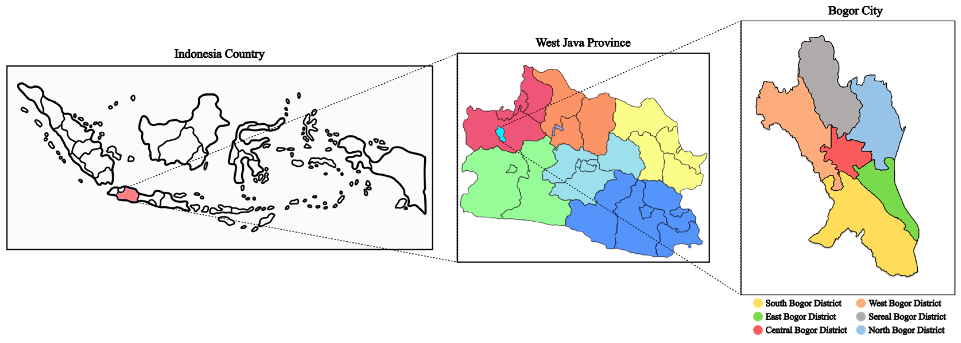
Rainfall data were obtained from Bogor, one of the major cities in Indonesia. Bogor was chosen as the location for rainfall data collection because it is known as the “Rain City”. Rainfall in Bogor can serve as an indicator of potential flooding in Indonesia’s capital, Jakarta. Figure 1 shows Bogor, which is located in West Java, Indonesia.
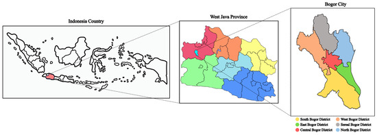
Figure 1.
Bogor maps of where the rainfall data were collected.
Studying rainfall in Bogor is crucial for several reasons beyond its impact on flooding in Jakarta. First, Bogor experiences high rainfall, which significantly affects local agriculture. The patterns of rainfall can help farmers better prepare for planting and harvesting, minimizing crop loss due to unexpected weather events. Second, understanding rainfall is essential for managing water resources, as Bogor’s precipitation contributes to the flow of water to nearby rivers, which are vital for surrounding communities. Understanding rainfall in Bogor helps not only with mitigating the effects on Jakarta but also with ensuring the city’s sustainable development, agricultural stability, and environmental health.
The daily rainfall data were collected from Bogor and converted to monthly data using two types of calendars: the Gregorian and lunar calendars. The conversion to monthly data was performed to capture the seasonal patterns. The monthly rainfall data for both the Gregorian and lunar calendars were analyzed using the spectral regression method. The result revealed that both datasets exhibited distinct seasonal indicated l pattern, with 12 periods, indicating that the rainfall followed a consistent yearly cycle.
Table 1 displays the outcomes of converting daily rainfall data from the Gregorian calendar to the lunar calendar. During the 22-year observation period, the Gregorian calendar consists of 273 months, while the whole lunar calendar consists of 286 months.

Table 1.
Calendar conversion results.
After the daily data were converted to both the Gregorian and lunar calendars, the time-series data for the lunar calendar were longer than that for the Gregorian calendar. The Gregorian calendar has 365 days, while the lunar calendar has only 355 days in a year. This difference results in a longer time series when using the lunar calendar.
3.2. Forecasting Result Comparison
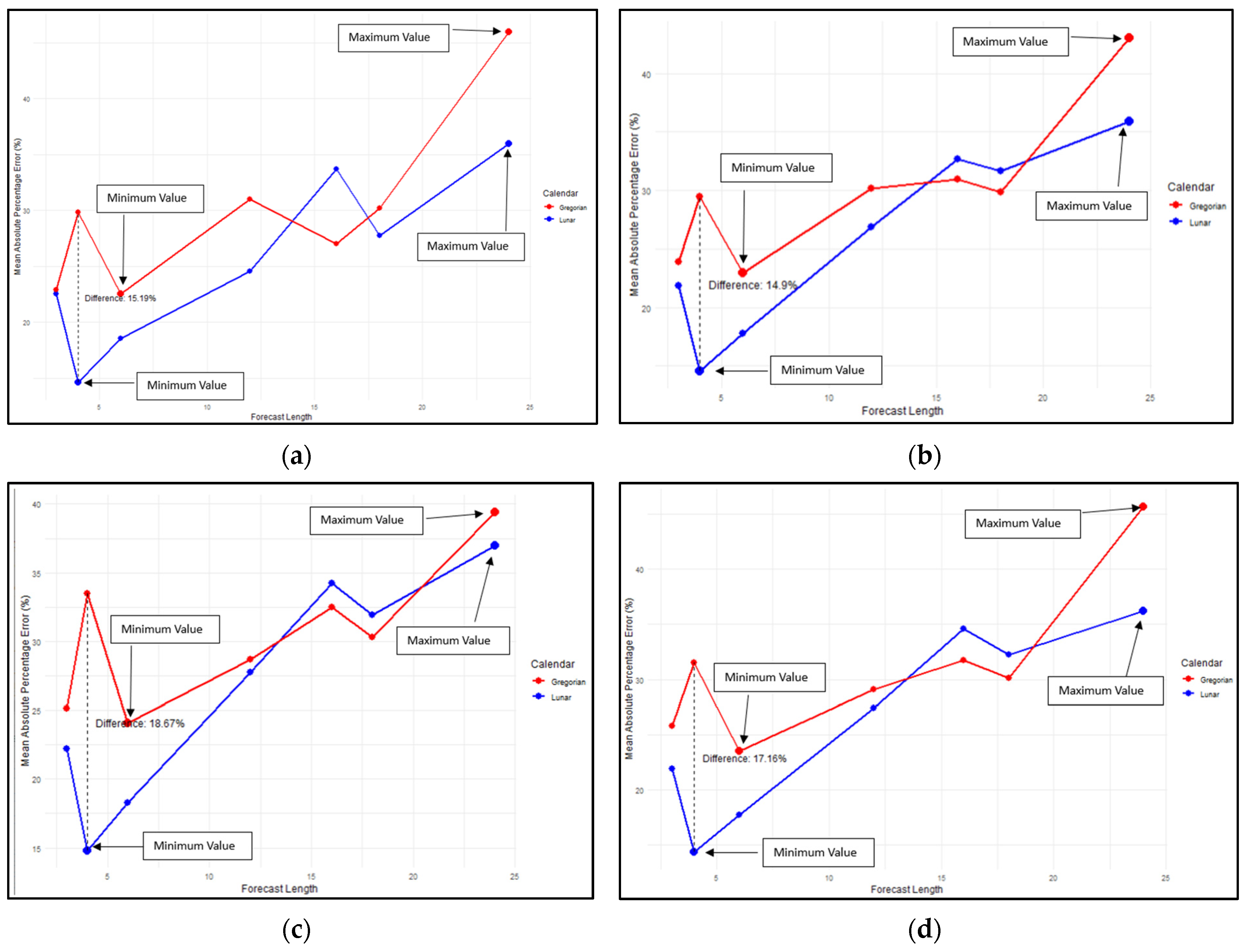
The comparison of forecasting based on two calendar systems is presented in Figure 2. As shown in Figure 2, the MAPE trend for all four methods across both calendar systems tends to increase as the forecast length extends. Forecasts based on the lunar calendar generally exhibited a lower MAPE than those based on the Gregorian calendar. Specifically, the MAPE for the lunar calendar was lower at forecast lengths of 3, 4, 6, and 12 months for the LSTM, 2-stacked LSTM, and 2-stacked BiLSTM methods, as illustrated in Figure 2a–d.
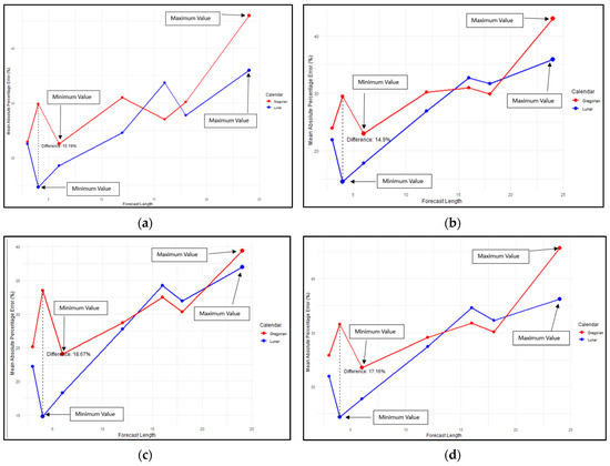
Figure 2.
Comparison of MAPE for lunar calendar-based forecasting and Gregorian calendar for the following: (a) LSTM; (b) 2-stacked LSTM; (c) BiLSTM; (d) 2-stacked BiLSTM methods.
For the BiLSTM method, at a forecast length of 12 months, the MAPE for both the lunar and Gregorian calendars was nearly identical. However, at forecast lengths of 16 and 18 months, the MAPE for the lunar calendar tended to be higher than that of the Gregorian calendar, particularly for the 2-stacked LSTM, BiLSTM, and 2-stacked BiLSTM methods. Interestingly, at a forecast length of 24 months, the lunar calendar exhibited a smaller MAPE.
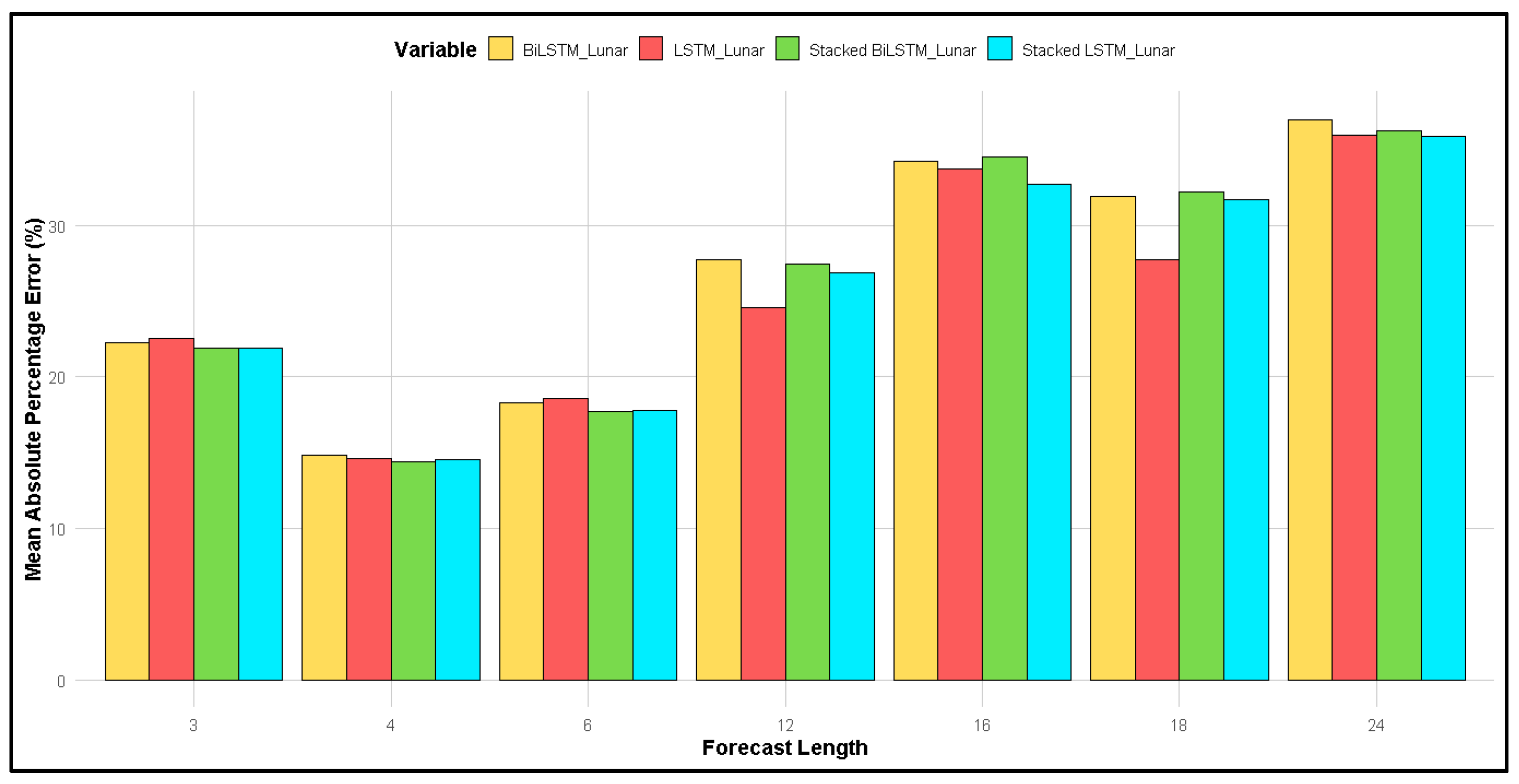
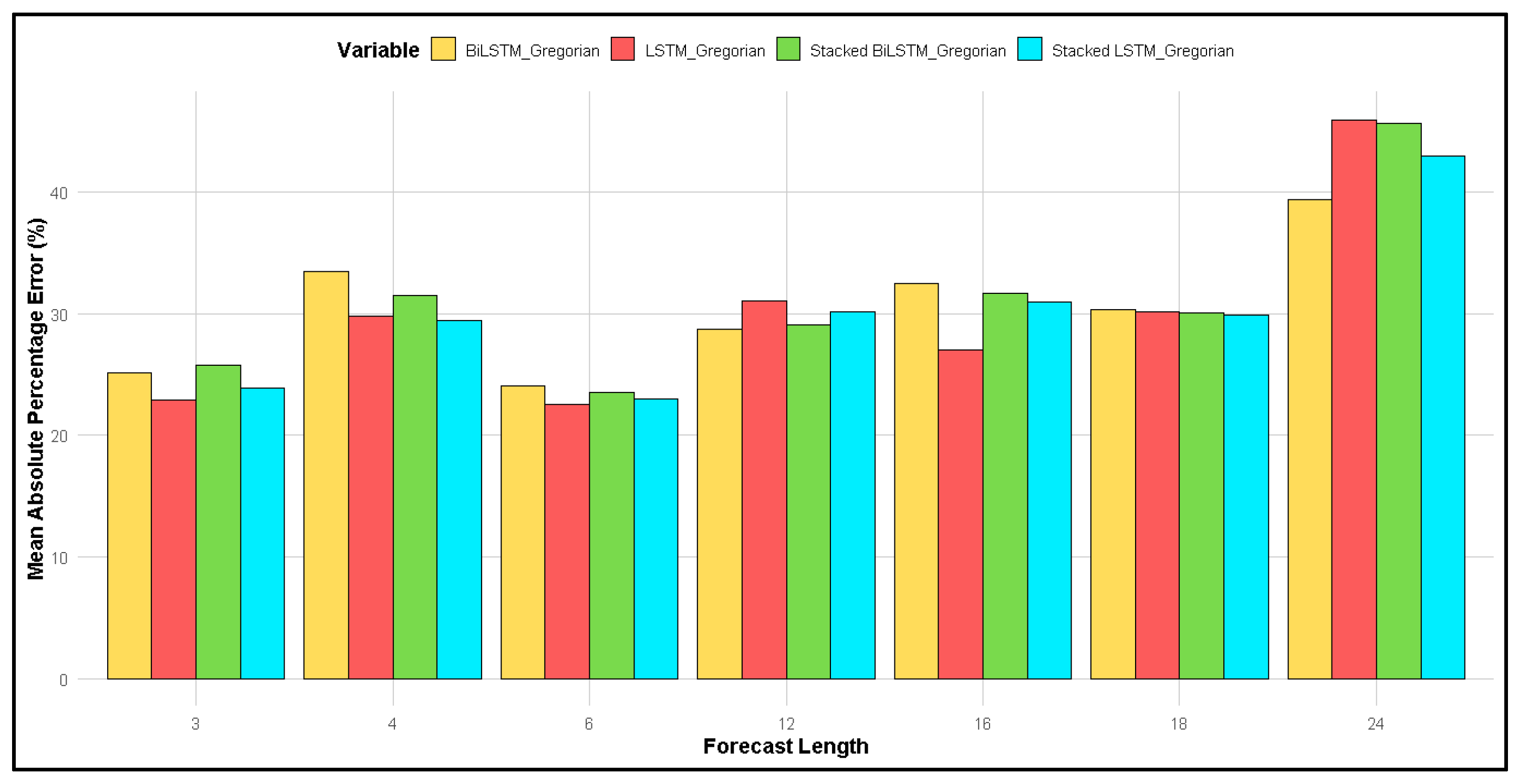
Figure 3 and Figure 4 compare the MAPE for forecasts using two different calendars: (3) the lunar calendar and (4) the Gregorian calendar, across forecast lengths of 3, 4, 6, 12, 16, 18, and 24 months.

Figure 3.
Comparison of MAPE for different forecast lengths for four different LSTM methods for forecasting based on the lunar calendar.

Figure 4.
Comparison of MAPE for different forecast lengths for four different LSTM methods for forecasting based on the Gregorian calendar.
Figure 3 shows that, for a forecast length of 4 months, the MAPE produced via all four methods was the smallest compared to other forecast lengths, while a forecast length of 24 months resulted in the highest MAPE.
On the other hand, for forecasts based on the Gregorian calendar (Figure 4), the smallest MAPE was observed at a forecast length of 6 months for all methods, with the largest MAPE occurring at 24 months. When comparing the two calendars, the MAPE for the lunar calendar was smaller than that for the Gregorian calendar at forecast lengths of 4 and 6 months.
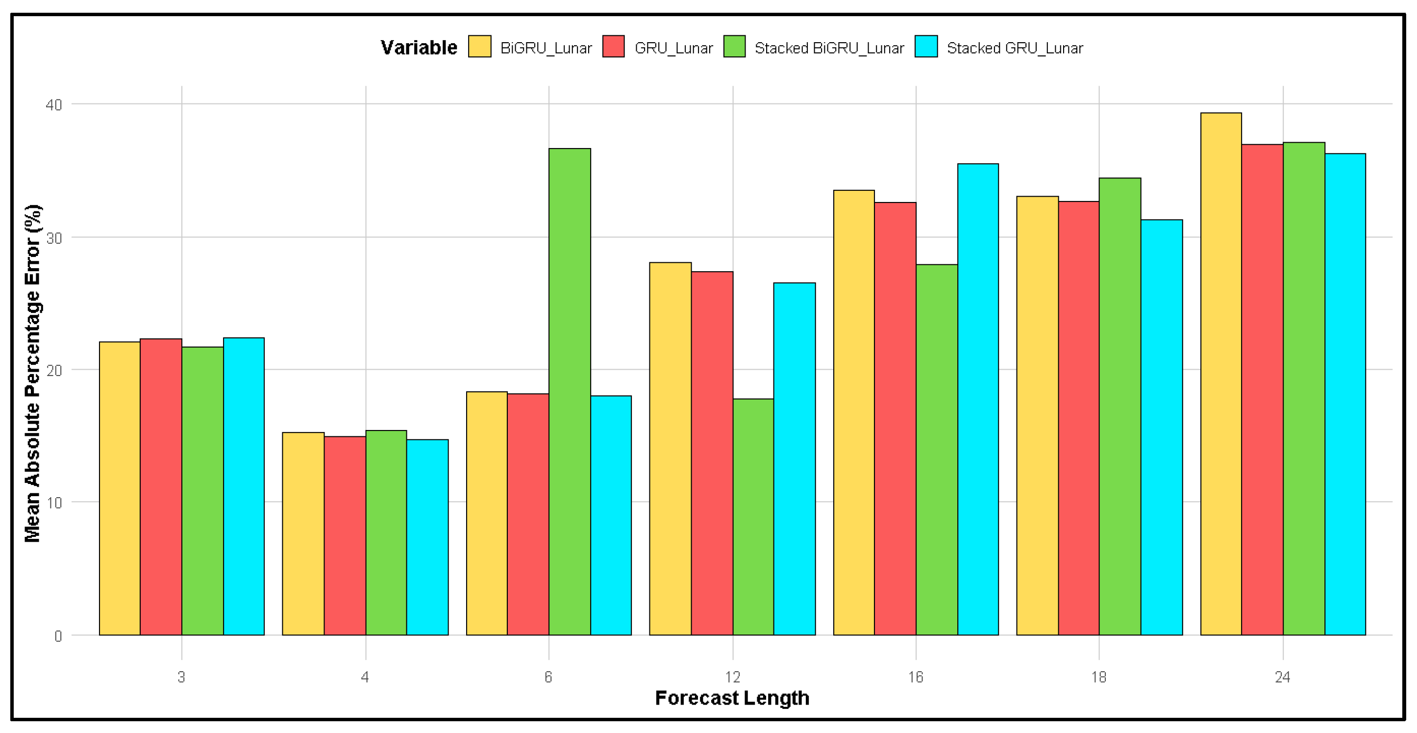
Figure 5 compares the MAPE of different methods: GRU, 2-stacked GRU, BiGRU, and 2-stacked BiGRU. Overall, the MAPE for the lunar calendar approach was generally smaller than that for the Gregorian calendar. Specifically, for forecast lengths of 3, 4, and 6 months, all four methods produced a smaller MAPE with the lunar calendar compared to the Gregorian calendar. For the BiGRU and 2-stacked BiGRU methods, the MAPE at a forecast length of 12 months was similar, typically ranging between 25 and 30%. However, at forecast lengths of 16 and 18 months, the MAPE for the lunar calendar was larger than that for the Gregorian calendar. In contrast, at a forecast length of 24 months, the MAPE for the Gregorian calendar was greater than that for the lunar calendar.
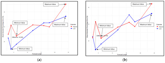
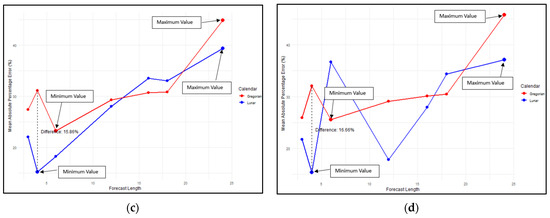
Figure 5.
Comparison of MAPE for lunar calendar-based forecasting and Gregorian calendar for the following: (a) GRU; (b) 2-stacked GRU; (c) BiGRU; (d) 2-stacked BiGRU methods.
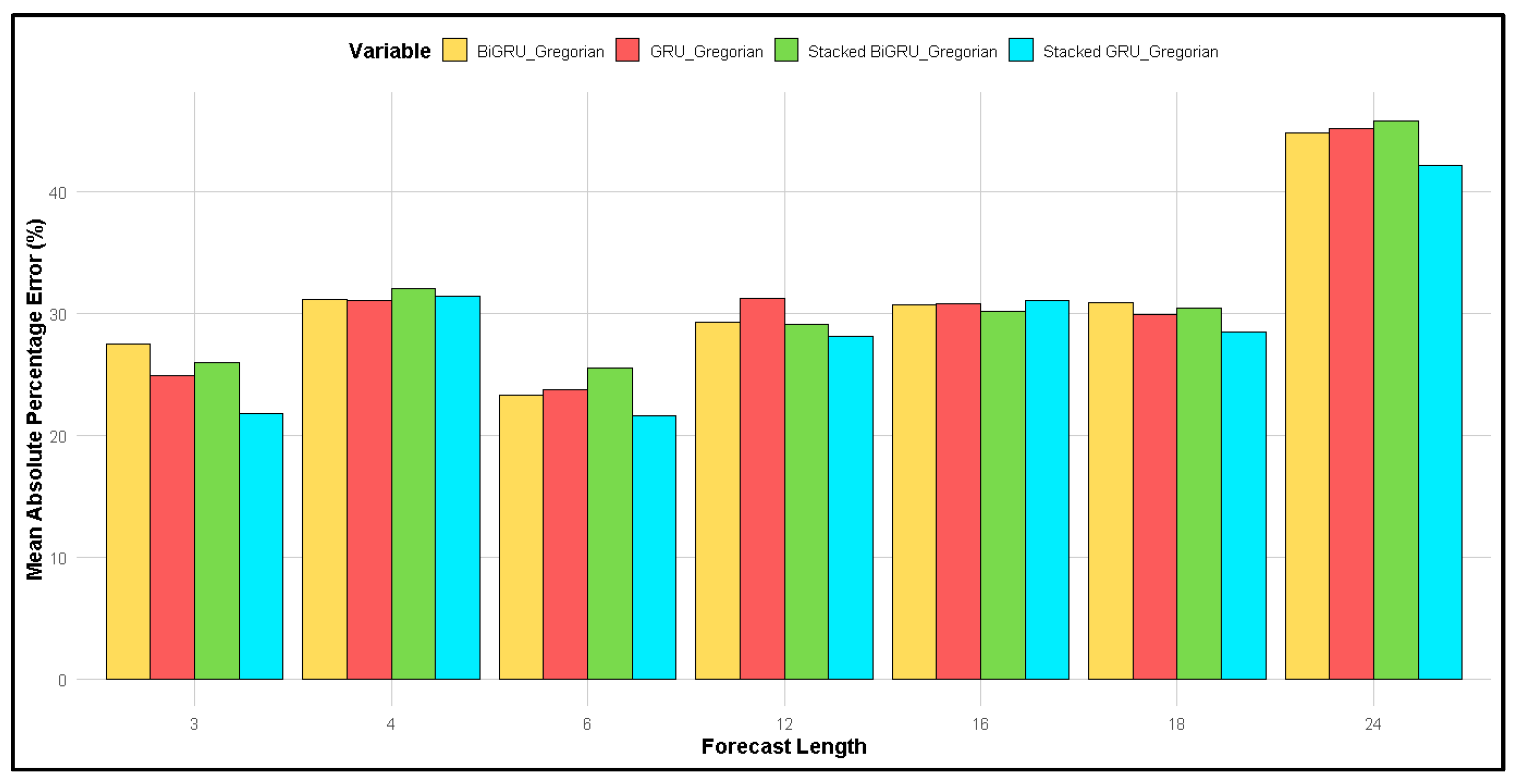
This comparison examines the MAPE for both the lunar and Gregorian calendars across four GRU method types: GRU, BiGRU, 2-stacked GRU, and 2-stacked BiGRU. As shown in Figure 6, the forecast length of 4 months yields the smallest MAPE, around 15%, while the forecast length of 24 months produces the highest MAPE, around 35%. In contrast, for the Gregorian calendar (Figure 7), the smallest MAPE occurs at forecast lengths of 3 and 6 months, approximately 25%, with the largest MAPE at 24 months, exceeding 40%. Overall, the MAPE for the lunar calendar was smaller than that of the Gregorian calendar at forecast lengths of 3, 4, 6, 12, and 24 months. However, at forecast lengths of 16 and 18 months, the MAPE values were relatively similar for both calendars.

Figure 6.
Comparison of MAPE for different forecast lengths for four different GRU methods for forecasting based on the lunar calendar.

Figure 7.
Comparison of MAPE for different forecast lengths for four different GRU methods for forecasting based on the Gregorian calendar.
In comparison (according to Table 2) to the lunar calendar, the forecasted values for the Gregorian calendar are typically larger in magnitude (more negative) for each n, which represents a particular data point. For example, when n = 3, the Gregorian forecasts range from −201.38 to −134.68, while the lunar predictions range from −37.06 to −17.53. This indicates that, compared to the lunar forecasts, the Gregorian predictions generally involve greater errors or discrepancies. When comparing the GRU (gated recurrent unit) and its variants (stacked GRU and BiGRU) to LSTM (long short-term memory) and its variants (stacked LSTM, BiLSTM, and stacked BiLSTM), LSTM models typically produce lower error values. For instance, LSTM yields an error of −37.06 for the lunar column when n = 3, while GRU produces a slightly smaller error of −19.46. In both the lunar and Gregorian calendars, stacked models (stacked LSTM, stacked BiLSTM, and stacked GRU) generally perform better (i.e., result in smaller errors) than their non-stacked counterparts. This suggests that increasing the number of layers in the model can reduce errors and improve accuracy. Although bidirectional models (BiLSTM and BiGRU) do not always outperform conventional LSTM or GRU models in terms of error size, they often provide reasonably acceptable results. However, BiLSTM or BiGRU might perform better than the conventional models at specific data points. For example, while the regular LSTM produces an error of −38.34 at n = 16 in the lunar calendar, BiLSTM and stacked BiLSTM show errors of −24.31 and −31.09, respectively. As the value of n increases, the forecasted values for all models generally show a trend of decreasing errors, indicating better performance at longer forecast horizons. This suggests that the model becomes more accurate when predicting data points farther from the training set.
Table 2.
Comparison of mean bias error (MBE).
The discrepancies across the models (Table 2) are particularly noticeable for the Gregorian calendar, where LSTM and BiLSTM show relatively consistent results, while some models, such as GRU and BiGRU, tend to forecast lower values.
A comparison of these two metrics (Table 3) revealed that the lunar calendar showed a slight overestimation in predictions (positive MBE) but performed with higher accuracy (lower MAPE). However, the Gregorian calendar showed a slight underestimation in prediction (negative MBE) and yielded larger prediction errors (higher MAPE). The lunar calendar model was more accurate in its predictions, with smaller errors, while the Gregorian calendar model had slightly larger errors and showed a tendency to underestimate the values.
Table 3.
Comparison of MBE and MAPE for training data.
4. Conclusions
The lunar calendar model demonstrated higher accuracy in its prediction, exhibiting smaller errors (MAPE and MBE (mean bias error) values), whereas the Gregorian calendar model had somewhat larger errors and tended to underestimate the values. The MAPE trend for the four methods and two calendars increases with forecast length, with lunar calendar-based forecasting generally yielding a lower MAPE than the Gregorian calendar. For the BiLSTM method, the MAPE at a forecast length of 12 months is similar for both calendars. However, at forecast lengths of 16 and 18 months, lunar calendar forecasts tend to show a larger MAPE compared to the Gregorian calendar. This study compares MAPE for forecasting using the lunar and Gregorian calendars across various forecast lengths, with the smallest MAPE observed at a forecast length of 4 months and the largest at 24 months. For the Gregorian calendar, the smallest MAPE occurs at forecast lengths of 3 and 6 months, while the largest is at 24 months. Figure 5 illustrates the MAPE of different methods: GRU, 2-stacked GRU, BiGRU, and 2-stacked BiGRU. The lunar calendar approach consistently shows a smaller MAPE than the Gregorian calendar for forecast lengths of 3, 4, and 6 months, while the BiGRU and 2-Stacked BiGRU methods produce similar MAPE values at the 12-month forecasts. The comparison of MAPE between the two calendars across the four GRU methods reveals that the smallest MAPE (15%) occurs at a forecast length of 4 months, with the largest MAPE (35%) at 24 months. For the Gregorian calendar, the smallest MAPE is observed at forecast lengths of 3 and 6 months, while the largest MAPE is at 24 months. Consequently, the analysis based on the lunar calendar tends to be more accurate, as the longer time-series data it provides offers more detailed insights. Therefore, the lunar calendar may lead to better analysis results compared to the Gregorian calendar. Model performance: Stacked models, such as stacked LSTM and stacked BiLSTM, generally outperform their non-stacked counterparts. Additionally, bidirectional models like BiLSTM and BiGRU frequently outperform conventional LSTM and GRU models. The Gregorian calendar data tend to show greater prediction errors than the lunar calendar, likely due to differences in time patterns or data properties. Although all models exhibit significant prediction errors, the variations among them help identify the most suitable models for this type of data. For these predictions, stacked LSTM and stacked BiLSTM models are likely to yield the best results.
Author Contributions
Conceptualization, G.D.; Methodology, D.Y.F.; Writing—original draft, B.H.; Supervision, G.R.S. All authors have read and agreed to the published version of the manuscript.
Funding
This research was funded by grant number 1652/UN6.3.1/PT.00/2024, and the APC was funded by Universitas of Padjadjaran.
Institutional Review Board Statement
Not applicable.
Informed Consent Statement
Not applicable.
Data Availability Statement
The data presented in this study are available upon request from the corresponding author.
Acknowledgments
The authors would like to acknowledge to Universitas Padjadjaran for funding this research.
Conflicts of Interest
The authors declare no conflicts of interest.
References
- Bartlein, P.J.; Shafer, S.L. Paleo Calendar-Effect Adjustments in Time-Slice and Transient Climate-Model Simulations (PaleoCalAdjust v1.0): Impact and Strategies for Data Analysis. Geosci. Model Dev. 2019, 12, 3889–3913. [Google Scholar] [CrossRef]
- Irfan, I. Comparative Study of Fazilet Calendar and Mabims Criteria on Determining Hijri Calendar. Al-Hilal J. Islam. Astron. 2023, 5, 99–116. [Google Scholar] [CrossRef]
- Hendikawati, P.; Subanar; Abdurakhman; Tarno. Optimal Adaptive Neuro-Fuzzy Inference System Architecture for Time Series Forecasting with Calendar Effect. Sains Malays. 2022, 51, 895–909. [Google Scholar] [CrossRef]
- Tang, T.; Jiao, D.; Chen, T.; Gui, G. Medium- and Long-Term Precipitation Forecasting Method Based on Data Augmentation and Machine Learning Algorithms. IEEE J. Sel. Top. Appl. Earth Obs. Remote Sens. 2022, 15, 1000–1011. [Google Scholar] [CrossRef]
- Archontoulis, S.V.; Castellano, M.J.; Licht, M.A.; Nichols, V.; Baum, M.; Huber, I.; Martinez-Feria, R.; Puntel, L.; Ordóñez, R.A.; Iqbal, J.; et al. Predicting Crop Yields and Soil-plant Nitrogen Dynamics in the US Corn Belt. Crop Sci. 2020, 60, 721–738. [Google Scholar] [CrossRef]
- Ceglar, A.; Toreti, A. Seasonal Climate Forecast Can Inform the European Agricultural Sector Well in Advance of Harvesting. npj Clim. Atmos. Sci. 2021, 4, 42. [Google Scholar] [CrossRef]
- Lala, J.; Tilahun, S.; Block, P. Predicting Rainy Season Onset in the Ethiopian Highlands for Agricultural Planning. J. Hydrometeorol. 2020, 21, 1675–1688. [Google Scholar] [CrossRef]
- Sodnik, J.; Mikoš, M.; Bezak, N. Torrential Hazards’ Mitigation Measures in a Typical Alpine Catchment in Slovenia. Appl. Sci. 2023, 13, 11136. [Google Scholar] [CrossRef]
- Adu-Gyamfi, A.; Poku-Boansi, M.; Darpoh, L.; Asibey, M.O.; Owusu-Ansah, J.K. Rainfall Challenges and Strategies to Improve Housing Construction in Sub-Saharan Africa: The Case of Ghana. Hous. Stud. 2023, 38, 1155–1190. [Google Scholar] [CrossRef]
- Zhang, J.; Zhong, D.; Wu, B.; Lv, F.; Cui, B. Earth Dam Construction Simulation Considering Stochastic Rainfall Impact. Comput. Civ. Infrastruct. Eng. 2018, 33, 459–480. [Google Scholar] [CrossRef]
- Golz, S.; Naumann, T.; Neubert, M.; Günther, B. Heavy Rainfall: An Underestimated Environmental Risk for Buildings? E3S Web Conf. 2016, 7, 08001. [Google Scholar] [CrossRef]
- Waqas, M.; Humphries, U.W.; Wangwongchai, A.; Dechpichai, P.; Ahmad, S. Potential of Artificial Intelligence-Based Techniques for Rainfall Forecasting in Thailand: A Comprehensive Review. Water 2023, 15, 2979. [Google Scholar] [CrossRef]
- Hammad, M.; Shoaib, M.; Salahudin, H.; Baig, M.A.I.; Khan, M.M.; Ullah, M.K. Rainfall Forecasting in Upper Indus Basin Using Various Artificial Intelligence Techniques. Stoch. Environ. Res. Risk Assess. 2021, 35, 2213–2235. [Google Scholar] [CrossRef]
- McGovern, A.; Elmore, K.L.; Gagne, D.J.; Haupt, S.E.; Karstens, C.D.; Lagerquist, R.; Smith, T.; Williams, J.K. Using Artificial Intelligence to Improve Real-Time Decision-Making for High-Impact Weather. Bull. Am. Meteorol. Soc. 2017, 98, 2073–2090. [Google Scholar] [CrossRef]
- Chambers, L.E.; Plotz, R.D.; Lui, S.; Aiono, F.; Tofaeono, T.; Hiriasia, D.; Tahani, L.; Fa'anunu, O.; Finaulahi, S.; Willy, A. Seasonal Calendars Enhance Climate Communication in the Pacific. Weather. Clim. Soc. 2020, 13, 159–172. [Google Scholar] [CrossRef]
- Ferrouhi, E.M.; Kharbouch, O.; Aguenaou, S.; Naeem, M. Calendar Anomalies in African Stock Markets. Cogent Econ. Financ. 2021, 9, 1978639. [Google Scholar] [CrossRef]
- Lessan, N.; Ali, T. Energy Metabolism and Intermittent Fasting: The Ramadan Perspective. Nutrients 2019, 11, 1192. [Google Scholar] [CrossRef]
- Oynotkinova, N.R. Calendar Rites and Holidays of the Altaians and Teleuts: Classification and General Characteristics. Sib. Filol. Zhurnal 2022, 332, 153–165. [Google Scholar] [CrossRef]
- Bell, W.R.; Hillmer, S.C. Modeling Time Series with Calendar Variation. J. Am. Stat. Assoc. 1983, 78, 526–534. [Google Scholar] [CrossRef]
- Ghamariadyan, M.; Imteaz, M.A. Monthly Rainfall Forecasting Using Temperature and Climate Indices through a Hybrid Method in Queensland, Australia. J. Hydrometeorol. 2021, 22, 1259–1273. [Google Scholar] [CrossRef]
- Kumar, D.; Singh, A.; Samui, P.; Jha, R.K. Forecasting Monthly Precipitation Using Sequential Modelling. Hydrol. Sci. J. 2019, 64, 690–700. [Google Scholar] [CrossRef]
- Heddam, S.; Ptak, M.; Zhu, S. Modelling of Daily Lake Surface Water Temperature from Air Temperature: Extremely Randomized Trees (ERT) versus Air2Water, MARS, M5Tree, RF and MLPNN; Elsevier: Amsterdam, The Netherland, 2020; Volume 588, ISBN 0000000280. [Google Scholar]
- Xie, J.; Hong, T. Load Forecasting Using 24 Solar Terms. J. Mod. Power Syst. Clean Energy 2018, 6, 208–214. [Google Scholar] [CrossRef]
- Li, G.; Yang, N. A Hybrid SARIMA-LSTM Model for Air Temperature Forecasting. Adv. Theory Simul. 2023, 6, 220502. [Google Scholar] [CrossRef]
- Sirisha, U.M.; Belavagi, M.C.; Attigeri, G. Profit Prediction Using ARIMA, SARIMA and LSTM Models in Time Series Forecasting: A Comparison. IEEE Access 2022, 10, 124715–124727. [Google Scholar] [CrossRef]
- Smyl, S. A Hybrid Method of Exponential Smoothing and Recurrent Neural Networks for Time Series Forecasting. Int. J. Forecast. 2020, 36, 75–85. [Google Scholar] [CrossRef]
- Darmawan, G.; Handoko, B.; Faidah, D.Y.; Islamiaty, D. Improving the Forecasting Accuracy Based on the Lunar Calendar in Modeling Rainfall Levels Using the Bi-LSTM Method through the Grid Search Approach. Sci. World J. 2023, 2023, 1863346. [Google Scholar] [CrossRef]
- Qiu, G.; Gu, Y.; Chen, J. Selective Health Indicator for Bearings Ensemble Remaining Useful Life Prediction with Genetic Algorithm and Weibull Proportional Hazards Model. Meas. J. Int. Meas. Confed. 2020, 150, 107097. [Google Scholar] [CrossRef]
- Liu, S.; Ji, H.; Wang, M.C. Nonpooling Convolutional Neural Network Forecasting for Seasonal Time Series with Trends. IEEE Trans. Neural Netw. Learn. Syst. 2020, 31, 2879–2888. [Google Scholar] [CrossRef]
- Braga, A.R.; Gomes, D.G.; Freitas, B.M.; Cazier, J.A. A Cluster-Classification Method for Accurate Mining of Seasonal Honey Bee Patterns. Ecol. Inform. 2020, 59, 101107. [Google Scholar] [CrossRef]
- Karevan, Z.; Suykens, J.A.K. Transductive LSTM for Time-Series Prediction: An Application to Weather Forecasting. Neural Netw. 2020, 125, 1–9. [Google Scholar] [CrossRef]
- Roy, D.K.; Sarkar, T.K.; Kamar, S.S.A.; Goswami, T.; Muktadir, M.A.; Al-Ghobari, H.M.; Alataway, A.; Dewidar, A.Z.; El-Shafei, A.A.; Mattar, M.A. Daily Prediction and Multi-Step Forward Forecasting of Reference Evapotranspiration Using LSTM and Bi-LSTM Models. Agronomy 2022, 12, 594. [Google Scholar] [CrossRef]
- Yin, J.; Deng, Z.; Ines, A.V.M.; Wu, J.; Rasu, E. Forecast of Short-Term Daily Reference Evapotranspiration under Limited Meteorological Variables Using a Hybrid Bi-Directional Long Short-Term Memory Model (Bi-LSTM). Agric. Water Manag. 2020, 242, 106386. [Google Scholar] [CrossRef]
- Kong, Z.; Zhang, C.; Lv, H.; Xiong, F.; Fu, Z. Multimodal Feature Extraction and Fusion Deep Neural Networks for Short-Term Load Forecasting. IEEE Access 2020, 8, 185373–185383. [Google Scholar] [CrossRef]
- Li, X.; Ma, X.; Xiao, F.; Xiao, C.; Wang, F.; Zhang, S. Time-Series Production Forecasting Method Based on the Integration of Bidirectional Gated Recurrent Unit (Bi-GRU) Network and Sparrow Search Algorithm (SSA). J. Pet. Sci. Eng. 2022, 208, 109309. [Google Scholar] [CrossRef]
- Johnson, R.K. Gregorian/Julian Calendar; Wiley: Hoboken, NJ, USA, 2011. [Google Scholar]
- Lee, K.W. Analysis of Solar and Lunar Motions in the Seonmyeong Calendar. J. Astron. Space Sci. 2019, 36, 87–96. [Google Scholar] [CrossRef]
- Gajic, N. The Curious Case of the Milankovitch Calendar. Hist. Geo. Space Sci. 2019, 10, 235–243. [Google Scholar] [CrossRef]
- Ando, H.; Shahjahan, M.; Kitahashi, T. Periodic Regulation of Expression of Genes for Kisspeptin, Gonadotropin-Inhibitory Hormone and Their Receptors in the Grass Puffer: Implications in Seasonal, Daily and Lunar Rhythms of Reproduction. Gen. Comp. Endocrinol. 2018, 265, 149–153. [Google Scholar] [CrossRef]
- Neri, C.; Schneider, L. Euclidean Affine Functions and Their Application to Calendar Algorithms. Softw. Pract. Exp. 2023, 53, 937–970. [Google Scholar] [CrossRef]
- Abdul Majid, A. Forecasting Monthly Wind Energy Using an Alternative Machine Training Method with Curve Fitting and Temporal Error Extraction Algorithm. Energies 2022, 15, 8596. [Google Scholar] [CrossRef]
- Meng, J.; Dong, Z.; Shao, Y.; Zhu, S.; Wu, S. Monthly Runoff Forecasting Based on Interval Sliding Window and Ensemble Learning. Sustainability 2023, 15, 100. [Google Scholar] [CrossRef]
- Zhang, H.; Nguyen, H.; Vu, D.-A.; Bui, X.-N.; Pradhan, B. Forecasting Monthly Copper Price: A Comparative Study of Various Machine Learning-Based Methods. Resour. Policy 2021, 73, 102189. [Google Scholar] [CrossRef]
- Hochreiter, S.; Schmidhuber, J. Long Short-Term Memory. Neural Comput. 1997, 9, 1735–1780. [Google Scholar] [CrossRef]
- Hochreiter, S.; Bengio, Y.; Frasconi, P.; Schmidhuber, J. Gradient Flow in Recurrent Nets: The Difficulty of Learning Long-Term Dependencies. In A Field Guide to Dynamical Recurrent Neural Networks; Kremer, S.C., Kolen, J.F., Eds.; IEEE Press: Piscatway, NJ, USA, 2001. [Google Scholar]
- Bengio, Y.; Simard, P.; Frasconi, P. Learning Long-Term Dependencies with Gradient Descent Is Difficult. IEEE Trans. Neural Netw. 1994, 5, 157–166. [Google Scholar] [CrossRef]
- Yu, Y.; Si, X.; Hu, C.; Zhang, J. A Review of Recurrent Neural Networks: LSTM Cells and Network Architectures. Neural Comput. 2019, 31, 1235–1270. [Google Scholar] [CrossRef]
- Dutta, K.K.; Poornima, S.; Sharma, R.; Nair, D.; Ploeger, P.G. Applications of Recurrent Neural Network: Overview and Case Studies. In Recurrent Neural Networks; CRC Press: Boca Raton, FL, USA, 2022; pp. 23–41. [Google Scholar]
- Cho, K.; van Merriënboer, B.; Gulcehre, C.; Bahdanau, D.; Bougares, F.; Schwenk, H.; Bengio, Y. Learning Phrase Representations Using RNN Encoder–Decoder for Statistical Machine Translation. In Proceedings of the 2014 Conference on Empirical Methods in Natural Language Processing (EMNLP), Doha, Qatar, 25–29 October 2014; Moschitti, A., Pang, B., Daelemans, W., Eds.; Association for Computational Linguistics: Stroudsburg, PA, USA; pp. 1724–1734. [Google Scholar]
- Salem, F.M. Gated RNN: The Gated Recurrent Unit (GRU) RNN. In Recurrent Neural Networks: From Simple to Gated Architectures; Springer International Publishing: Cham, Switzerland, 2022; pp. 85–100. ISBN 978-3-030-89929-5. [Google Scholar]
- Mateus, B.C.; Mendes, M.; Farinha, J.T.; Assis, R.; Cardoso, A.M. Comparing LSTM and GRU Models to Predict the Condition of a Pulp Paper Press. Energies 2021, 14, 6958. [Google Scholar] [CrossRef]
- Zhang, W.; Li, H.; Tang, L.; Gu, X.; Wang, L.; Wang, L. Displacement Prediction of Jiuxianping Landslide Using Gated Recurrent Unit (GRU) Networks. Acta Geotech. 2022, 17, 1367–1382. [Google Scholar] [CrossRef]
- Chung, J.; Gulcehre, C.; Cho, K.; Bengio, Y. Empirical Evaluation of Gated Recurrent Neural Networks on Sequence Modeling. arXiv 2014, arXiv:1412.3555. [Google Scholar]
- Bahdanau, D.; Cho, K.; Bengio, Y. Neural Machine Translation by Jointly Learning to Align and Translate. arXiv 2016, arXiv:1412.3555. [Google Scholar]
- Boulanger-Lewandowski, N.; Bengio, Y.; Vincent, P. Modeling Temporal Dependencies in High-Dimensional Sequences: Application to Polyphonic Music Generation and Transcription. arXiv 2012, arXiv:1206.6392. [Google Scholar]
- Mienye, I.D.; Swart, T.G.; Obaido, G. Recurrent Neural Networks: A Comprehensive Review of Architectures, Variants, and Applications. Information 2024, 15, 517. [Google Scholar] [CrossRef]
- Sahar, A.; Han, D. An LSTM-Based Indoor Positioning Method Using Wi-Fi Signals. In Proceedings of the 2nd International Conference on Vision, Image and Signal Processing, Las Vegas, NV, USA, 27–29 August 2018; ACM: New York, NY, USA, 2018; pp. 1–5. [Google Scholar]
- Schuster, M.; Paliwal, K.K. Bidirectional Recurrent Neural Networks. IEEE Trans. Signal Process. 1997, 45, 2673–2681. [Google Scholar] [CrossRef]
- Graves, A.; Schmidhuber, J. Framewise Phoneme Classification with Bidirectional LSTM and Other Neural Network Architectures. Neural Netw. 2005, 18, 602–610. [Google Scholar] [CrossRef] [PubMed]
- Graves, A.; Mohamed, A.-R.; Hinton, G. Speech Recognition with Deep Recurrent Neural Networks. In Proceedings of the 2013 IEEE International Conference on Acoustics, Speech and Signal Processing, Vancouver, BC, Canada, 26–31 May 2013; pp. 6645–6649. [Google Scholar]
- Cui, Z.; Ke, R.; Pu, Z.; Wang, Y. Stacked Bidirectional and Unidirectional LSTM Recurrent Neural Network for Forecasting Network-Wide Traffic State with Missing Values. Transp. Res. Part C Emerg. Technol. 2020, 118, 102674. [Google Scholar] [CrossRef]
- Rathore, M.S.; Harsha, S.P. An Attention-Based Stacked BiLSTM Framework for Predicting Remaining Useful Life of Rolling Bearings. Appl. Soft Comput. 2022, 131, 109765. [Google Scholar] [CrossRef]


Disclaimer/Publisher’s Note: The statements, opinions and data contained in all publications are solely those of the individual author(s) and contributor(s) and not of MDPI and/or the editor(s). MDPI and/or the editor(s) disclaim responsibility for any injury to people or property resulting from any ideas, methods, instructions or products referred to in the content. |
© 2025 by the authors. Licensee MDPI, Basel, Switzerland. This article is an open access article distributed under the terms and conditions of the Creative Commons Attribution (CC BY) license (https://creativecommons.org/licenses/by/4.0/).