Article

BWFER-YOLOv8: An Enhanced Cascaded Framework for Concealed Object Detection

by
Khalid Ijaz
1,
Ikramullah Khosa
1,*,
Ejaz A. Ansari
1,
Syed Farooq Ali
2,
Asif Hussain
3,* and
Faran Awais Butt
4
1
Department of Electrical and Computer Engineering, COMSATS University Islamabad, Lahore 54000, Pakistan
2
Department of Computer Science, School of Systems and Technology, University of Management and Technology, Lahore 54770, Pakistan
3
Department of Electrical Engineering, School of Engineering, University of Management and Technology, Lahore 54770, Pakistan
4
Center for Communication Systems and Sensing, King Fahd University of Petroleum and Minerals, Dhahran 31261, Saudi Arabia
*
Authors to whom correspondence should be addressed.
Appl. Sci. 2025, 15(2), 690; https://doi.org/10.3390/app15020690
Submission received: 5 December 2024 / Revised: 6 January 2025 / Accepted: 7 January 2025 / Published: 12 January 2025

Abstract

:
Contact-free concealed object detection using passive millimeter-wave imaging (PMMWI) sensors is a challenging task due to a low signal-to-noise ratio (SNR) and nonuniform illumination affecting the captured image’s quality. The nonuniform illumination also generates a higher false positive rate due to the limited ability to differentiate small hidden objects from the background of images. Several concealed object detection models have demonstrated outstanding performance but failed to combat the above-mentioned challenges concurrently. This paper proposes a novel three-stage cascaded framework named BWFER-YOLOv8, which implements a new alpha-reshuffled bootstrap random sampling method in the first stage, followed by image reconstruction using an adaptive Wiener filter in the second stage. The third stage uses a novel FER-YOLOv8 architecture with a custom-designed feature extraction and regularization (FER) module and multiple regularized convolution (Conv_Reg) modules for better generalization capability. The comprehensive quantitative and qualitative analysis reveals that the proposed framework outperforms the state-of-the-art tiny YOLOv3 and YOLOv8 models by achieving 98.1% precision and recall in detecting concealed weapons. The proposed framework significantly reduces the false positive rate, by up to 1.8%, in the detection of hidden small guns.

1. Introduction

An impeccable concealed threat detection system delivers contact-free security screening across various places, including airport checkpoints, warehouses, sports stadiums, religious congregations, and concurrent productions [1,2,3]. The detection of concealed weapons and improvised explosive devices employed by terrorists has been a demanding milestone, underscoring the need to strengthen global counter-terrorism efforts to ensure invulnerable public security systems [4]. The Global Terrorism Index report of 2024 indicates that terrorism led to 8352 deaths in 2023, identifying a 22 percent increase from the previous year, especially in two countries, i.e., Burkina Faso and Pakistan, as shown in Figure 1 [5]. Hence, improvements in the efficiency of existing concealed object detection (COD) systems are required to address a diverse array of hidden threats, encompassing weapons, explosives, and contraband.
Traditional security screening equipment, such as X-ray machines, infrared-based imaging systems, and metal detectors, have certain constraints. For example, infrared-based imaging systems fail to detect things hidden behind baggy garments [6,7]. However, X-rays have negative effects on the health of people in real-world scenarios [8,9,10]. Furthermore, metal detectors are vulnerable to insensitivity issues caused by non-metallic or tiny objects [11]. The above shortcomings have been eliminated to a large extent by using a terahertz (THz)-wave imaging system [12]. THz technologies can operate in two modes: passive or active. PMMW imaging technologies have gained a positive reputation since they exert no risk to human health [13,14,15]. PMMW sensors penetrate through non-metallic materials convincingly when compared to the aforementioned screening methods [16,17,18].
Despite the benefits of PMMW systems, PMMW systems experience enormous complications. The performance of PMMW systems deteriorates because the image datasets acquired from PMMW imaging screening systems struggle with low SNR and contrast, resulting in picture fuzziness [12]. Furthermore, PMMW imaging systems suffer from environmental noise and illumination problems due to complex light environments, unconstrained conditions, and view-point variations [19]. The above-stated drawbacks make detection one of the most fundamental and intimidating tasks in computer vision (CV) and artificial intelligence (AI).
Recent advances in CV, AI, and machine learning (ML) approaches have led to novel methods for quick, contact-free, and robust identification of concealed objects in PMMW imaging systems [20,21]. Unfortunately, by addressing one of the above-mentioned issues independently in a single study, the state-of-the-art (SOTA) ML, AI, and CV algorithms boost the performance of the COD system. However, the CV concerns mentioned above may concurrently affect the data obtained from the PMMW imaging equipment. Therefore, the SOTA ML, AI, and CV algorithms can show elevated false positive rates. As a result, this study proposes a novel three-stage cascade idea to develop a new algorithm that combats every CV challenge simultaneously.
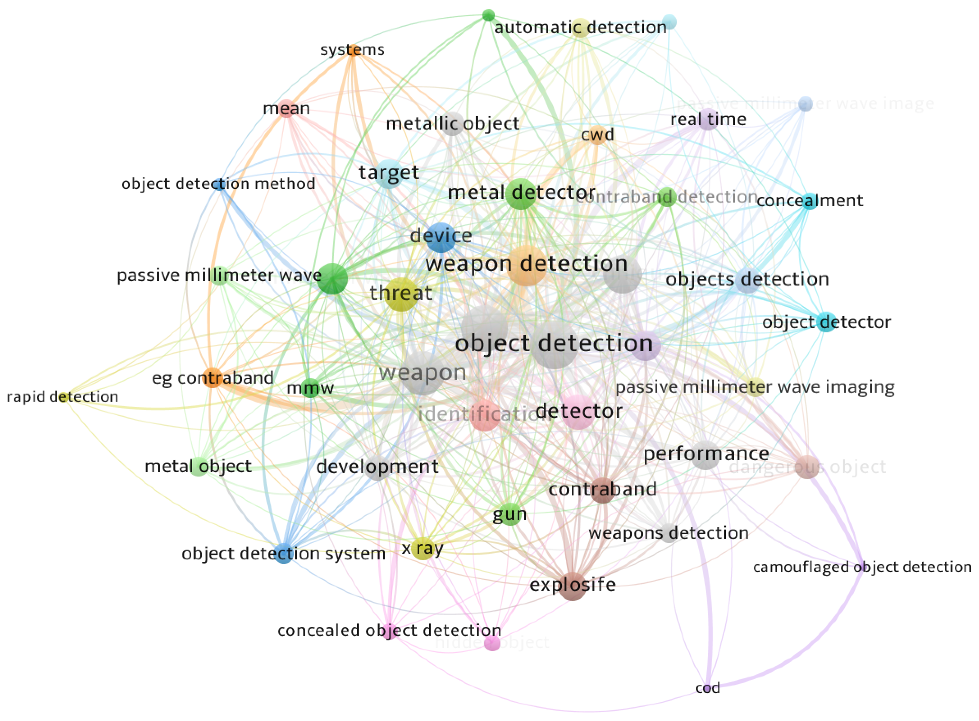
Furthermore, a bibliometric analysis of research articles published after 1990 demonstrates the research gap in the existing literature. The extensive literature survey reveals that few studies on weapon identification have been performed using traditional approaches, as seen in the blue cluster in Figure 2. However, the profound knowledge of the dull brown and dull yellow clusters of the bibliometric analysis emphasizes the severe necessity for rigorous study in the field of concealed weapon detection (CWD) employing PMMW imaging systems, since the words “cwd” and “passive millimeter wave imaging” are very dim as compared to other keywords in the dull brown and dull yellow clusters, respectively. To address the above-stated research gaps, the current work concentrates on CWD, employing a PMMW system, especially on detecting concealed small weapons with more accuracy by overcoming low signal-to-noise ratio, noise, illumination, and view-point variation problems.
The present study develops a unique BWFER-YOLOv8 framework for attaining high true positive (TP) and low false positive (FP) rates by addressing the signal-to-noise ratio, internal noise, and illumination issues. For the first time, the proposed framework exploits the strengths and potential of the adaptive Wiener filter (WF), the novel alpha-reshuffled bootstrap random sampling ( α -R BRS) method, and an improved YOLOv8 architecture for CWD. Extensive experiments reveal that the new framework enhances the TP rate by 6% and lowers the FP rate by up to 1.8% when compared to the tiny SOTA YOLOv3 architecture. Considering the above-mentioned discussion, the main contributions of the research paper can be summarized as follows.
  • Recent studies have demonstrated little emphasis on CWD performance for tiny weapons, allowing opportunity for improvement in the detection of concealed small weapons. The proposed study addresses the common CV challenges to improve CWD performance, such as low SNR, illumination, and view-point variations, concurrently. The above-mentioned issues have never been addressed concurrently.
  • The proposed framework deploys an adaptive WF to remove noise in the CWD dataset. Moreover, the WF efficiently executes data enhancement by improving the SNR and reducing illumination problems. To the best of the authors’ knowledge, the adaptive WF has not yet been applied to CWD systems.
  • A novel α -R BRS method is introduced to expand the CWD dataset. The proposed preprocessing technique enhances the accuracy of the proposed CWD framework.
  • The FER module has been added in the new enhanced YOLOv8 version, which comprises a 1 × 1 convolutional layer and dropout layer. The 1 × 1 convolutional layer is deployed to enhance the capability of feature extraction to detect small guns and to reduce the FP rate.
  • ConvModule in the SOTA YOLOv8 has been replaced by the Conv_Reg module in the recommended FER-YOLOv8 algorithm. The Conv_Reg and FER modules efficiently address the overfitting issue in the detection of small weapons as a dropout layer is instigated in both modules.
  • The proposed framework has been assessed on different evaluation metrics such as TP, FP, and mean average precision (mAP) to demonstrate the superiority of the proposed framework as compared to existing frameworks.
The remainder of the paper is organized as follows: Section 2 describes a detailed literature review; Section 3 presents a comprehensive suggested methodology; Section 4 demonstrates the configurations of various models and hyperparameter settings required for simulations; Section 5 discusses the evaluation metrics used for quantitative and qualitative analyses; Section 6 presents an in-depth quantitative and qualitative analysis of the obtained simulation results; and Section 7 concludes the paper with future research directions.

2. Related Work

The conventional approach to detecting objects is to segregate the three important regions, which are the background, body, and threats, from MMW images by applying K-means clustering. However, the K-means algorithm detects unconnected areas that do not possess metallic threats while detecting potential threats. To remove the problem of detecting unconnected areas as a metallic threat, the Active Shape Model (ASM) was developed to detect concealed objects inside the body [22]. However, the accuracy of the ASM model is not up to the desired level. The accuracy of CWD was improved by implementing the Gaussian mixture model (GMM), which segmented the image and characterized the background, threat regions, and body more accurately as compared to the ASM [23]. But the GMM also generates unconnected body segmentation. Moreover, the ASM and GMM techniques also fail to remove background noise from MMW images.
Furthermore, the accuracy of the CWD process was improved by eliminating noise from MMW images and then performing image segmentation using local binary fitting. The two main algorithms of image denoising, non-local means and iterative steering kernel regression, were also employed. The experiments revealed that the correctness of the segmentation of threats and background regions had been improved as compared to ASM and GMM, surpassing the precision of the COD. Although the precision and detection rate of COD reached up to 93%, the algorithm was computationally inefficient due to higher time complexity and low performance when exposed to high-resolution images [24].
The above-discussed CV and image processing techniques also suffer from diffraction limits and low intensity levels. To combat the above-mentioned drawbacks, global and local segmentation techniques were developed to detect suspicious objects in blurry grayscale images [25]. The above architecture is very complicated and was tested on a small dataset, which consisted of only two types of threats. In contrast to multi-level segmentation, a fast two-stage algorithm based on denoising and mathematical morphology was proposed in [26]. However, the proposed fast two-stage algorithm compromised on the FP rate. To improve the FP rate, a new way of initializing GMM parameter estimation was employed in multi-level concealed object segmentation systems [27,28]. Nevertheless, the above segmentation-based approach did not perform well on low-SNR MMW images with blurred boundaries.
To address the above-stated defect, a patch-based mixture of Gaussian low-rank matrix factorization (patch-based MoG-LRMF) was developed. Still, shadow or uneven illumination generates fusion of the objects and background area, which degrades the COD performance [29]. Wavelet fusion techniques were also presented to improve the quality of MMW images; these removed the uneven illumination problem by decomposing the image into pyramid sequences for CWD [30,31]. The efficacy of the COD algorithm was enhanced by applying a concept of disintegration of “featured regions”, which resolved the drawbacks of conventional methods, even considering low-SNR MMW images with blurred boundaries. However, the above method is not suitable for CWD because of a lower extraction capability for precise information about the contours of hidden objects. To mitigate the above drawback, Otsu’s algorithm and multi-thresholding techniques were used [32,33]. However, the above Otsu’s algorithm and multi-thresholding techniques have a high computational cost and are affected by non-stationary noise.
The development of ML classification algorithms such as support vector machines (SVM), with the integration of Haar filters and LBP, led to remarkable progress in detecting and localizing potential threats accurately. The TP and FP detection rates were also improved to a desirable extent [34,35,36]. Even though the proposed classifiers surpassed previous methods, image noise still has a powerful impact on the ML classifiers, which restricts classifiers to an average detection score no better than 68%. To boost the average detection score and to reduce the FP rate of CWD, deep learning (DL) frameworks were then employed. One of the main techniques of DL involved the attainment of visible imagery (VI) and MMW image datasets as a pre-requisite to achieve highly precise segmentation [17]. The preliminary deep neural network (DNN) models have an issue of becoming stuck in local optima during optimization in the case of binary images present in MMW imagery datasets. In contrast to DNN models, a convolutional neural network (CNN) has a great tendency to separate useful features from the images automatically by converging the optimizer to a minimum loss function [37].
CNN models manifested promising results for the detection of concealed weapons. Other SOTA CNN-based segmentation architectures were also presented, such as Segnet and Multi-scale Segnet CNN, which enhanced the performance of CWD [38,39]. Different region-based CNN architectures, such as faster region-based convolutional neural network (R-CNN), were also presented, in which the CNN was used to extract features and then region proposals were recorded from the input image in the form of anchors and bounding boxes [40,41]. However, an overfitting issue was discovered when CNN models were employed with inadequate parameters. To address the overfitting issue, a semantic segmentation algorithm was developed with expand–contract dilation, which made the effective receptive field larger and reduced a large number of parameters [3,42]. The CNN-based architectures discussed above failed to combat the issue of pose variation in CWD. A symmetry-driven Siamese network was presented for CWD to resolve the issue of pose variation [43].
Although the CNN-based architectures discussed above and different versions of the R-CNN architectures improved the accuracy of concealed object detection, they were ineffective for the detection of forbidden small objects [44,45,46,47]. For the detection of small concealed objects, a multisource aggravation transformer (MATR) model was invented. The MATR model was composed of self-attention and cross-attention mechanisms to extract spatial and contextual details across the images with integration of the selective context module [48]. Though the transformer model paved a new way to raise the COD performance, the distance between the instrument receiver and target led to noise in the image reconstruction. To reduce the effect of noise due to the distance between the target and the receiver, the raw data from frequency-modulated continuous wave (FMCW) radars were captured and trained using ML and DL techniques, which surprisingly enhanced the accuracy of COD [49]. However, the setup of FMCW radars was complicated and costly. Hence, a low-cost MMW radar system of 77 GHz was implemented, using multi-scale filtering and geometric (MSFG) augmentation to detect concealed weapons [50,51,52]. But the interference of environmental noise in the background of the images and the elevated time consumption of the MSFG algorithm restricted the use of the proposed algorithm in a real-life scenario.
To counter the complex background issues and environmental noise and to lessen the time complexity of the algorithm, a combination of transformers and convolutional networks was deployed [53]. A task-aligned detection transformer was also introduced to increase the classification and detection accuracy [54]. However, transformer networks require high computational resources on large training data for faultless CWD systems. Therefore, other approaches, such as weakly supervised 2D pose adaptation-based segmentation, weight label correction, and spatio-temporal weighted methods, were developed. The above methods achieved SOTA performance [55,56,57]. Regarding the above CWD networks, spatio-temporal and weight-labeling models are complex models to capture spatial and temporal features. Moreover, they are more prone to overfitting issues. Hence, new segmentation techniques were introduced using CNN, DL, and transfer learning [58,59,60,61].
The aforementioned segmentation approaches yielded compelling findings for CWD. However, random noise, complex backgrounds, and occlusion all had a negative impact on the effectiveness of segmentation algorithms. As a result, the next revolution in CWD systems relied on SOTA You Only Look Once (YOLO) designs, particularly YOLOv3 and YOLOv7, few-shot learning with YOLO, and wavelet-transform architectures, to reduce the effect of noise and improve TP and FP detection rates [1,62,63,64,65,66,67]. The word cloud shown in Figure 3 depicts the trend in CWD designs and frameworks after 2021. The bigger and bolder words of CNN, R-CNN, segmentation, and transformer networks indicate that the above methods were extensively employed in CWD applications. However, the aforementioned constraints have resulted in the invention of YOLO architectures for efficient CWD systems. The word cloud pattern also indicates that YOLOv3 and YOLOv7 have been investigated to a lesser extent. The YOLOv3 and YOLOv7 models attained higher FP rates (up to 7%), providing the opportunity to develop a new YOLOv8 version. The new proposed FER-YOLO v8 version obtains a higher TP rate while decreasing the FP rate by reducing noise, lighting, and pose variation concerns. The current study aims to use the abilities of the new FER-YOLOv8 version by including the FER module and modifying the convolutional modules in YOLOv8 when applied to grayscale images for CWD.

3. Materials and Methods

The current section describes the suggested method for properly classifying and detecting hidden weapons in an image. The proposed method also improves the efficacy of locating a hidden pistol, having higher precision and accuracy. The proposed method uses the power of the WF, α -R BRS approach, and the new FER-YOLOv8 architecture to extract significant local and global features from the PMMW image dataset in order to identify and localize the concealed gun. The proposed and SOTA models are trained and validated using PMMW imaging datasets collected with the SAIR-U imaging equipment [68]. A description of the dataset is given in the following subsection.

3.1. Materials

3.1.1. Dataset Overview

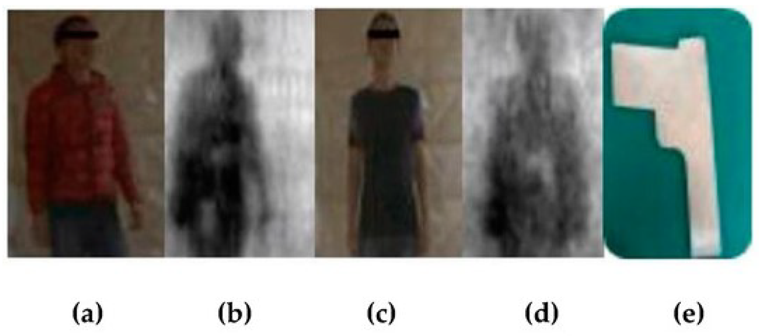
The PMMW imaging dataset comprises 1618 diverse images retrieved from the internet: (www.mdpi.com/1424-8220/20/6/1678/s1, accessed on 20 February 2024). The PMMW real-time imager was used to acquire the aforementioned dataset [68]. Figure 4a,c depict optical pictures of the data gathered by the examinee while wearing various thicknesses of clothes. Figure 4b,d illustrates the corresponding PMMW images. According to the reflection properties of the materials in the ka band, the human body’s reflectivity is lower than that of metal, hence the white block with high reflectivity on the human body in the image is contraband from the examinee’s experimental pistol.
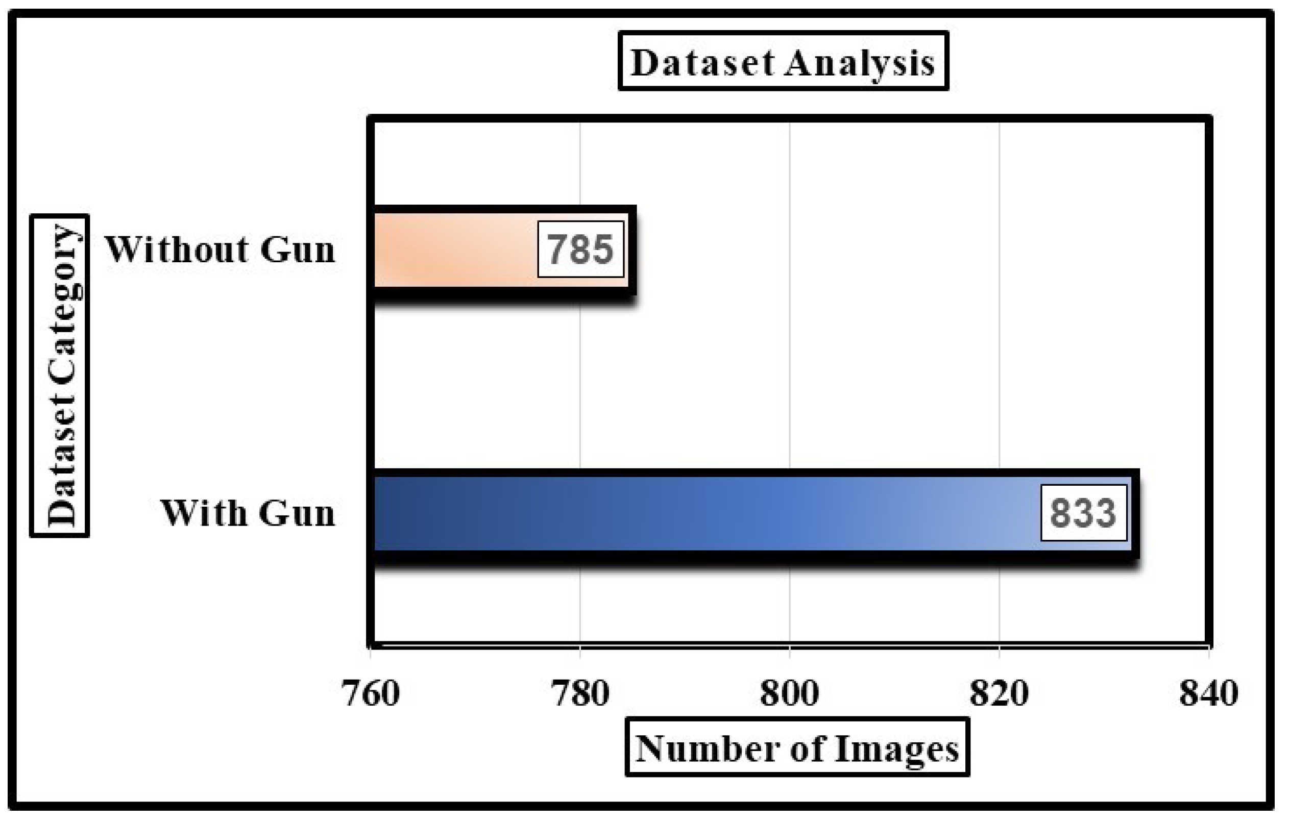
Out of 1618 images, 833 have a metal pistol on the human body. While 785 pictures do not show a metal gun, as shown in Figure 5. To demonstrate the reliability of the proposed technique, the examinee gathered sample data while wearing several layers of clothes and carrying the metal gun item at various temperatures and imaging speeds. This addressed the impacts of temperature, imaging speed, and garment thickness on the target detection, as well as the frequency band. Afterwards, preprocessing was performed to make the dataset utilizable.

3.1.2. Data Preprocessing

To obtain a higher TP rate and accuracy with the suggested framework, noisy and low-quality images were eliminated from the gun category, leaving 1590 useful images. The imbalanced dataset may cause a bias towards the majority class during training, reducing performance for the minority class in the detection and localization problem; the aforementioned dataset was preprocessed further. As a result, 10 images that did not possess a gun were added to the without gun category using a random sampling approach. To address the class imbalance problem, 10 images were removed from the gun category using random sampling. Following preprocessing, each category had 795 images. Algorithm 1 is demonstrated below.
Algorithm 1 Class Balancing using Random Sampling
Require: 
Imbalanced dataset χ ¯
Ensure: 
Balanced dataset with equal number of positive and negative samples χ
  1:
Sorting:  P , N —Positive & Negative samples.
  2:
for i in χ ¯  do
  3:
    P SortPositiveSamples ( χ ¯ )
  4:
    N SortNegativeSamples ( χ ¯ )
  5:
end for
  6:
Balancing:  P , N —Positive & Negative samples.
  7:
for i in P do
  8:
    P RemovePositiveSamples ( P , N p = No . of samples to remove )
  9:
end for
10:
for i in N do
11:
    N AddNegativeSamples ( N , N n = No . of samples to add )
12:
end for
13:
Aggregation: Obtaining Final dataset χ
14:
for each i in ( N + P )  do
15:
    χ CollectPositiveNegativeSamples ( P , N )
16:
end for
Figure 5. Class-imbalanced PMMW image dataset.
Applsci 15 00690 g005

3.2. Methods

3.2.1. Problem Statement

The purpose is to classify an image as class + 1 (positive) if an image includes a concealed gun and class 0 (negative) otherwise. The proposed study also intends to localize where the concealed object is on the human body. Let χ = { X 1 , X 2 , , X n } be the image dataset, where n represents the total number of images present in the dataset. The goal is to learn from all “n” images contained in χ a function f χ ( n ) = M with the lowest generalization error, where M indicates the trained model and parameters.
The function f χ ( n ) allocates each picture a set of pixels, X i , where threats are located, or an empty set if no concealed gun is present. The problem under consideration is related to object detection and localization. The idea is to use deep learning techniques to address the given problem. The function f χ ( n ) has two functionalities: detecting possible threats and determining which regions provide a true hazard. Validation is used to estimate the generalization error of the function learned from the entire dataset χ .

3.2.2. Alpha-Reshuffled Bootstrap Random Sampling Method

The excellence of the proposed framework hinges on the enrichment of the high-quality PMMW imaging dataset. Moreover, deep CNN models, such as YOLOv8, require a large quantity of data to train for accurate detection of concealed guns. Furthermore, to guarantee the accuracy and reliability of the detection model for CWD systems, the old and new enhanced data must be consistent, i.e., the ensembled average of the new enhanced dataset and the old dataset should be the same. The main issue with data augmentation in COD systems is that labels do not always match up with the objects’ updated locations. Inaccurate model training might result from any mismatch between the label and the concealed item. As a result, the PMMW imaging dataset was enlarged fourfold using a novel α -R BRS approach in this study.
The suggested α -R BRS approach randomly resamples image data from the original data source and then adds the resampled data into the original data source. This ensures that the distribution of classes in the new enriched dataset remains the same as in the original. As previously mentioned, χ = { X 1 , X 2 , , X n } is the image dataset, which constitutes positive- and negative-labeled samples. The process of how positive- and negative-sample subsets were extracted from χ , inculcating two subsets, i.e., P i and D i , is shown in Figure 6. Hence, χ = P i D i . P i and D i can be mathematically expressed as in Equations (1) and (2), respectively:
P i = { p p χ ,   p is a positive sample }
D i = { d d χ ,   d is a negative sample }
Assume P i and D i have τ and ϵ samples, respectively. The objective is to improve the data α times so that the new dataset will be α χ . For this, the P i and D i subsets are expanded α times. The data from P i and D i are randomly resampled to create j-sample subsets, with α = j . The resampled positive and negative images are increased to α τ and α ϵ . If P 1 , P 2 ,…, P j represent various subsets of the positive samples, then P j P i .
Similarly, for the negative samples, D 1 , D 2 ,…, D j represent various subsets of negative samples, then D j D i . Afterwards, all the data subsets are aggregated as mathematically demonstrated in Equation (3):
A = j = 1 α P i P j j = 1 α D i D j
The dataset is then reshuffled to avoid short-term biasing in the batches during training. Let A ¯ be the reshuffled data, then A ¯ = shuffle (A). The reshuffled data are mathematically expressed as in Equation (4):
A ¯ = { P 1 * , P 2 * , , P j * , D 1 * , D 2 * , , D j * }
where { P 1 * , P 2 * , , P j * , D 1 * , D 2 * , , D j * } is a permutation of { P 1 , P 2 , , P j , D 1 , D 2 , , D j } .
So, the new enriched PMMW imaging dataset will be α χ and α χ = A ¯ and α χ χ . Suppose the means of χ and α χ is denoted by μ x and μ d , respectively. Therefore, the mean μ d can be calculated as in Equation (5):
μ d = Mean { mean ( P 1 * ) , mean ( P 2 * ) , , mean ( P j * ) , mean ( D 1 * ) , mean ( D 2 * ) , , mean ( D j * ) }
Assume that mean ( P 1 * ) = b 1 , mean ( P 2 * ) = b 2 , , mean ( P j * ) = b n k , mean ( D 1 * ) = b n k + 1 , , mean ( D j * ) = b n . Then, B will be a new set containing subsets b 1 , b 2 , , b n . Hence, B can also be written as B = { b 1 , b 2 , b 3 , , b n } . Then, the arithmetic mean μ d can also be mathematically written as in Equation (6):
μ d = 1 n i = 1 n b i
Theorem 1.
Consider χ to be the original dataset such that χ = { X 1 , X 2 , , X n } , then the new augmented dataset, α χ , resampled from the α-R BRS technique, is consistent with χ.
Proof 
The arithmetic mean of the original dataset can be mathematically demonstrated as μ x = 1 n i = 1 n x i , where n is the number of images and x i is the pixel mean of the ith image in the original dataset. Similarly, the arithmetic mean of the α -R BRS-expanded dataset can be mathematically demonstrated as μ d = 1 n i = 1 n b i , where b i represents the pixel mean of the ith image in the new dataset. The expected value of μ d can be written as in Equation (7):
E [ μ d ] = E 1 n i = 1 n b i
Since each b i is sampled from the original dataset χ , the expected value of b i is approximately the mean of the original dataset χ . The expected value of b i may not be exactly the same as the mean of the original dataset because of randomness in selecting the samples. Thus, Equation (8) is
E [ μ d ] μ x
Hence, on average, the mean of the original dataset will be approximately equal to the mean of the α -R BRS-expanded dataset, as shown in Equation (9):
E [ μ d ] E 1 n i = 1 n b i μ x
Therefore, the above Equation (9) concludes that the new augmented dataset, α χ , resampled from the α -R BRS technique, is consistent with χ . □

3.2.3. Adaptive Wiener Filter

The adaptive Wiener filter alters the filter output based on the image’s local variance. The final objective is to reduce the mean square error between the restored and original images. The adaptive Wiener filter impressively suppresses the internal noise of the sensors, which are perturbed due to the physical limitations of sensors, as compared to other filters. The adaptive Wiener filter also improves the SNR of an image and hence removes the degradation and illumination problem. The adaptive Wiener filtering particularly restores the image’s edges and high-frequency regions. The selection of the optimal kernel size is always inevitable for proper implementation of the adaptive Wiener filter in a CWD system. Therefore, different combinations of kernel sizes were used, such as 1, 2, 3, 4, and 5. Of these, a kernel size of 5 shows better results. Consider the filtering of images distorted by signal-perturbed noise, then the degradation of the images can be described by Equation (10):
y ( i , j ) = x ( i , j ) h ( i , j ) + n ( i , j )
where y ( i , j ) represents the noisy image, x ( i , j ) is the noise-free image, n ( i , j ) is the noise owing to the limits of the physical setup, and h ( i , j ) is the operator matrix of linear spatial distortions with kernel elements of the point spread function (PSF). The linear operator h ( i , j ) is frequently spatially invariant, therefore the distortions can be represented by a convolution operator. The adaptive Wiener filter is then used to solve problem mentioned in the above Equation (10). The working of the adaptive Wiener filter can be realized in the frequency domain as Fourier transform and inverse Fourier transform operations, as expressed in Equation (11):
s ^ = F 1 F { u } H * ( ω ) | H ( ω ) | 2 + P n ( ω ) / P s ( ω )
where H ( ω ) is the Fourier transformation of PSF h ( x , y ) , P n ( ω ) is the spectral density of the noise, and P s ( ω ) is the spectral density of the signal; ( · ) * denotes complex conjugation.
A comparison of filtered and original images is shown in Figure 7. Figure 7a–d depict the ground truth, whereas Figure 7e–h show the filter-enhanced images. Wiener-filtered images have a much higher SNR and eliminate image inhomogeneity. The pictures obtained after implementing the Wiener filter are smooth images.

3.2.4. YOLOv8 Algorithm

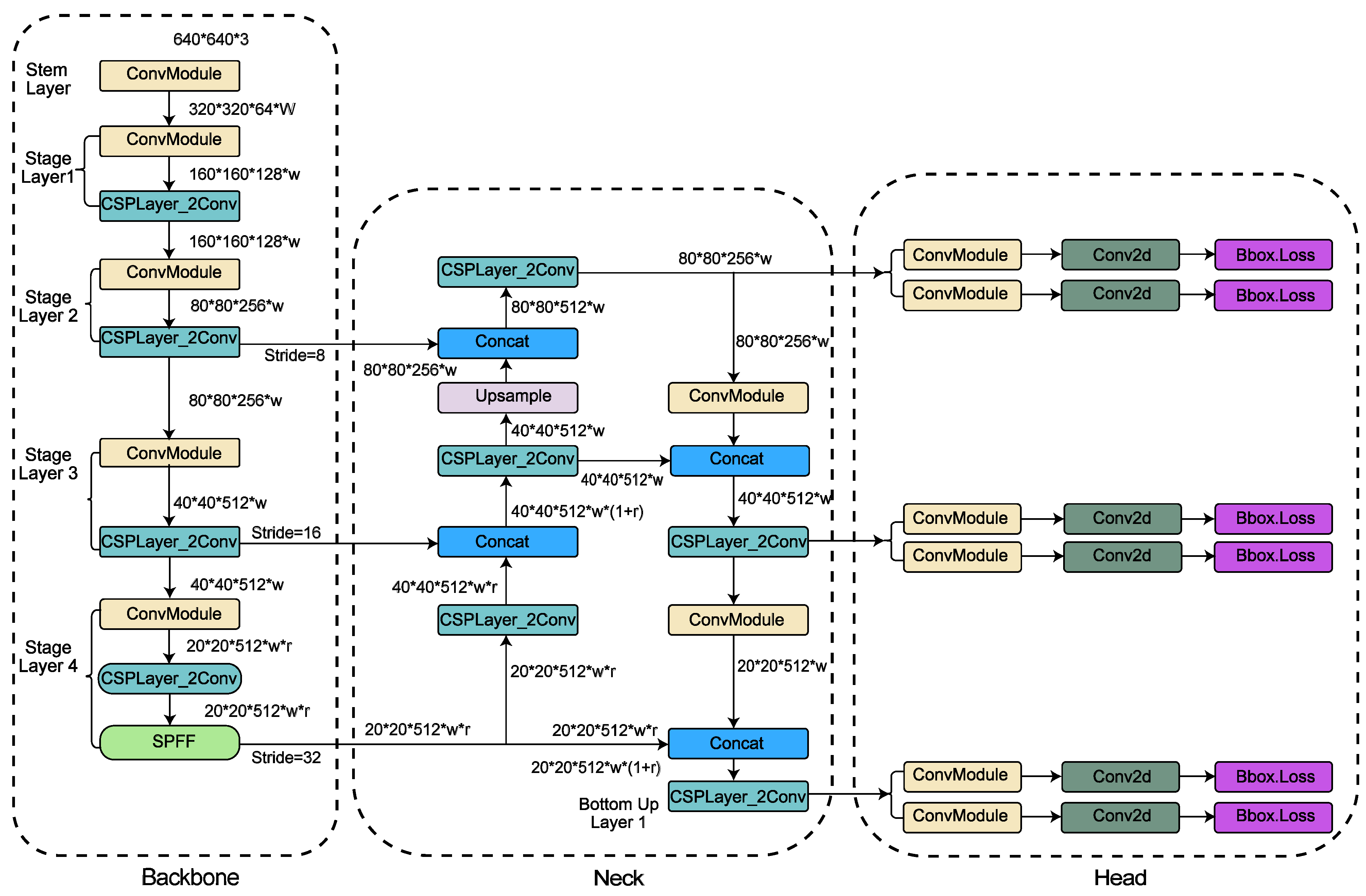
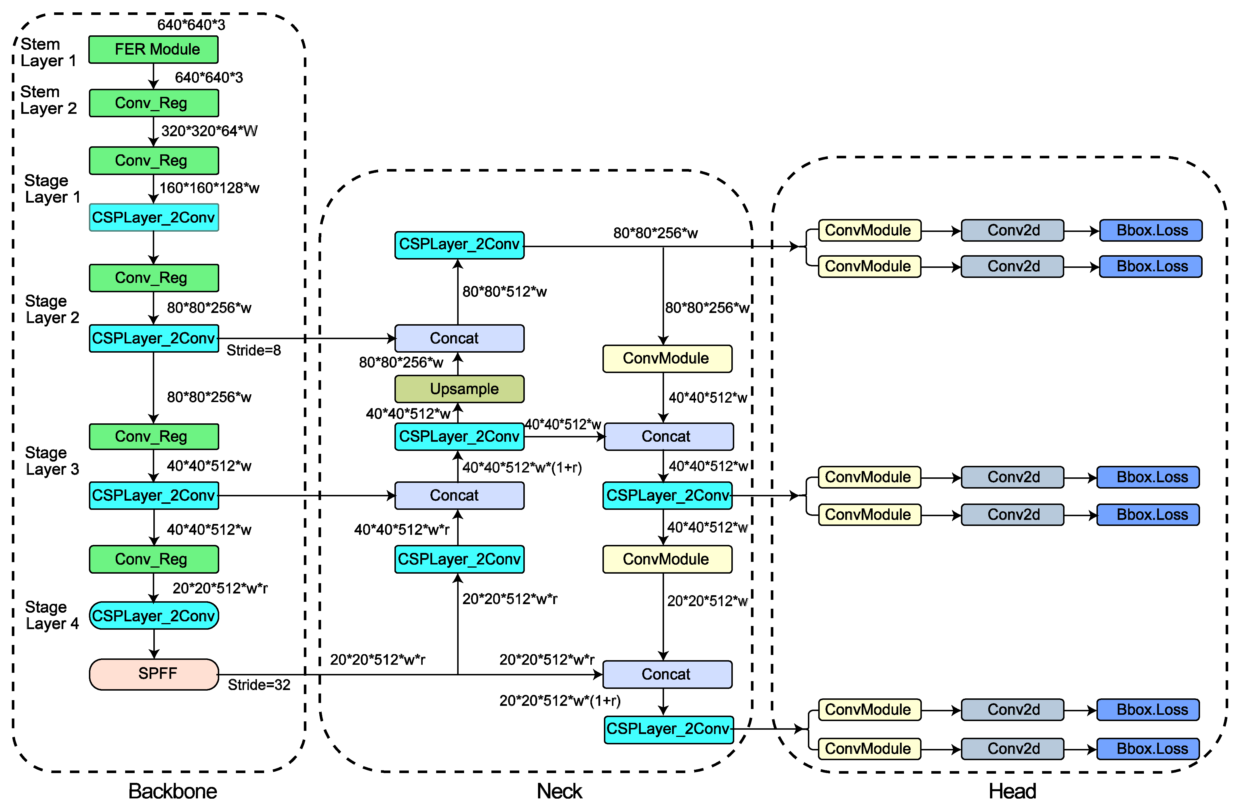
The four primary parts of the SOTA YOLOv8 network architecture are the input, the backbone network, feature enhancement (neck), and the decoupling head (head). An adaptive anchor frame calculation, adaptive grayscale filling, and mosaic data augmentation are some of the main improvements on the input side. The YOLOv8 backbone network uses the CSP (Cross Stage Partial) concept and lightweight CSPLayer_2Conv module. Finally, the widely used SPPF (Spatial Pyramid Pooling with Factorized Convolutions) module completes the backbone network, adding to its strong feature extraction capabilities. The neck section uses PAN-FPN (Path Aggregation Network–Feature Pyramid Network) for feature improvement. PAN-FPN is a bi-directional pathway. Three down-sampled inputs are integrated using this feature pyramid network via channel fusion via up sampling. In the end, three branches receive the output, which is supplied in the direction of the decoupling head. The separation of the prediction and regression branches is the responsibility of the decoupling head. Both the category and localization components are used in the loss computation in the regression branch. The binary cross-entropy loss function is used in the adoption of Varifocal Loss for category loss. The components of loss associated with localization are the CIoU (Complete IoU) and DFL (Distribution Focal Loss). The overall YOLOv8 network architecture is visually depicted in Figure 8.
Using cross-entropy, DFL describes the position of the target detection frame as a global distribution. Equation (12) demonstrates the network’s capacity to rapidly focus on the target spot. Interval orders are denoted by y i and y i + 1 , the output of the network’s sigmoid function is represented by s i and s i + 1 , and y is a label.
DFL S i , S i + 1 = y i + 1 y log S i + y y i log S i + 1

3.2.5. Proposed FER-YOLOv8 Algorithm

The SOTA YOLOv8 architecture increases the capacity for detection but is unable to significantly lower the FP rate. Before entering the ConvModule of the conventional YOLOv8, the pixel representation of the background and the pixel representation of the local region containing suspicious objects can be captured while maintaining the same image size to prevent information loss. Furthermore, when applied to a grayscale PMMW imaging dataset, the excessive number of parameters in the SOTA YOLOv8 architecture may cause an overfitting problem. As a result, this paper suggests a new YOLOv8 model named FER-YOLOv8. The FER module in the new FER-YOLOv8 design is placed at the beginning of the backbone portion. Each ConvModule in the backbone and neck sections is replaced with a new module, named Conv_Reg. Conv_Reg module implants a dropout layer for regularization after convolutional layer. The new advancements in the proposed FER-YOLOv8 architecture are highlighted in the green block in Figure 9.

3.2.6. FER Module

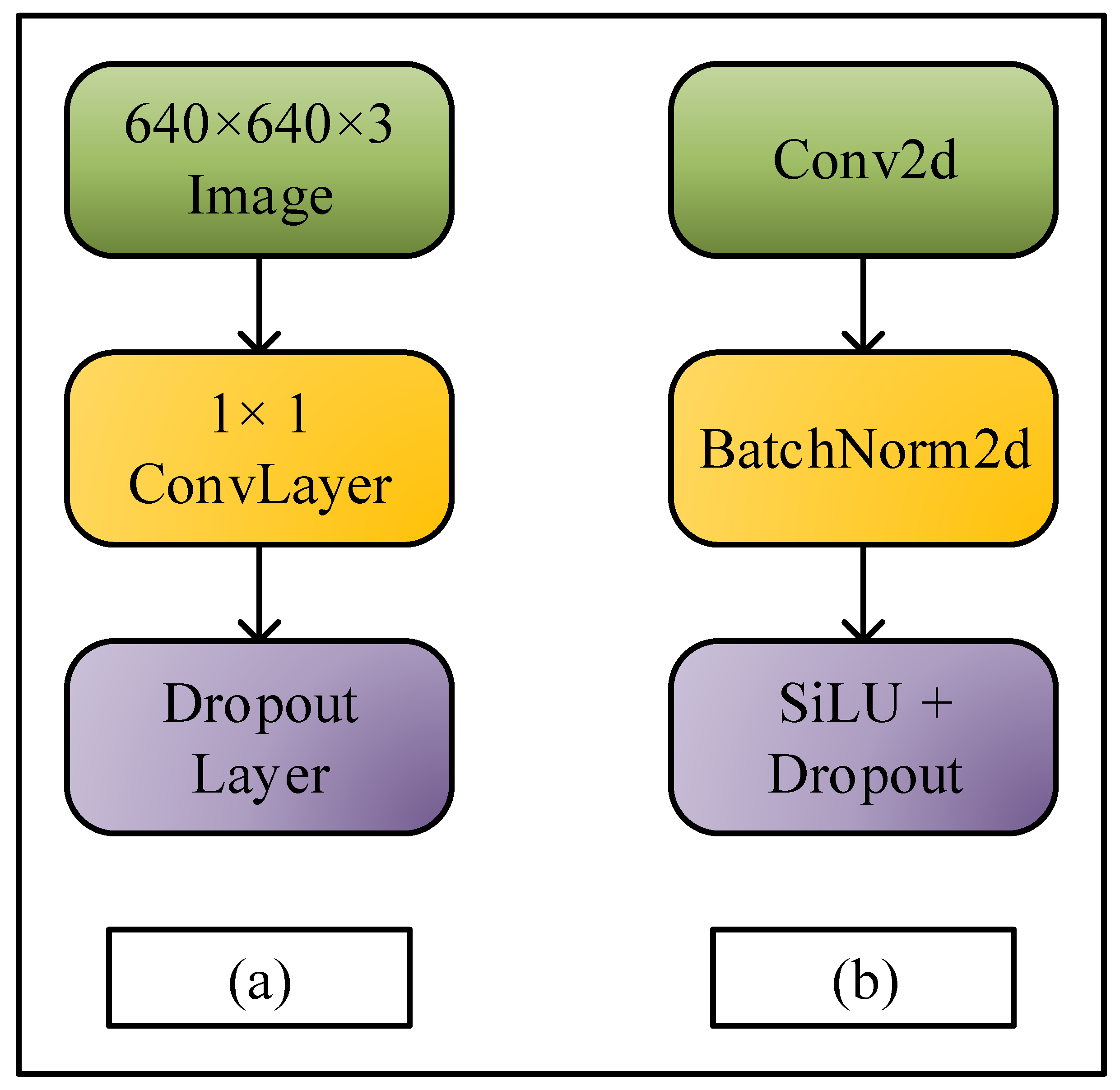
The FER module consists of a lightweight convolutional layer of filter size 1 with 1 filter and a dropout layer, as shown in Figure 10a. The 1 × 1 convolutional layer with sigmoid-weighted linear unit (SiLU) activation function boosts the feature extraction capability by distinguishing the pixel representations (intensities) of the region of interest, which contains the suspicious guns, from the pixel representations of the background. Moreover, the input and output size of the FER module ensure no spatial information loss during capturing the crucial features. In addition to this, the dropout layer after the 1 × 1 convolutional layer in the FER module also combats the overfitting issue in the proposed YOLOv8 architecture. The convolution operation can be mathematically expressed as in Equation (13):
l i , j , 0 = m = K + 1 2 K + 1 2 n = K + 1 2 K + 1 2 c = 0 C 1 X i + m , j + n , c . W m , n , c , o
where Y represents the output tensor, and i, j, and o are the row, column, and output channel indices of the output tensor Y, respectively. As the input image is in grayscale, the output channel is one. W ∈ R K × K × C × O is a 4D tensor, where O is the number of output channels. K is the size of the convolution kernel. This operation is carried out for i = 0 , 1 , 2 , , W ¯ K , j = 0 , 1 , 2 , , H ¯ K , and c = 0 , 1 , 2 , , C 1 , where the filter W can fit into the input tensor X. The simplified convolution procedure can be written as in Equation (14):
Y O = W K , K , C O X K , K , C
For instance, the dropout effect is denoted by D. Y represents L y . The gradients during backpropagation, L W and L X , after considering the effect of dropout are calculated as in Equation (15):
L W = D . Y X K , K , C T , L X = D . W K , K , C O o Y
The output Y O of the convolution layer is passed through the dropout layer to regularize the feature map. For instance, the dropout rate is δ , the output of the FER module is Y, so Y can be written as in Equation (16):
Y = δ . ( Y O ) O R Y = δ . ( W K , K , C O X K , K , C )

3.2.7. Conv_Reg Module

The new Conv_Reg module is displayed in Figure 10b. Again, a dropout layer is added after the ConvModule of the YOLOv8 algorithm to add regularization to enhance the generalization capability of the proposed architecture. The parameters of the convolutional layers such as kernel size, stride, and padding in the Conv_Reg module remain the same as in the backbone and neck sections of the SOTA YOLOv8 algorithm. The SiLU activation function is used to enhance the feature extraction capability of the Conv_Reg module.
The mathematical representations of the convolution and dropout operations in the Conv_Reg module are the same as described in Equations (14)–(16). The updated DFL loss in the proposed FER-YOLOv8 algorithm can be mathematically expressed as in Equation (17):
DFL S i , S i + 1 = D . ( y i + 1 y log S i + y y i log S i + 1 )

3.2.8. Proposed Research Framework

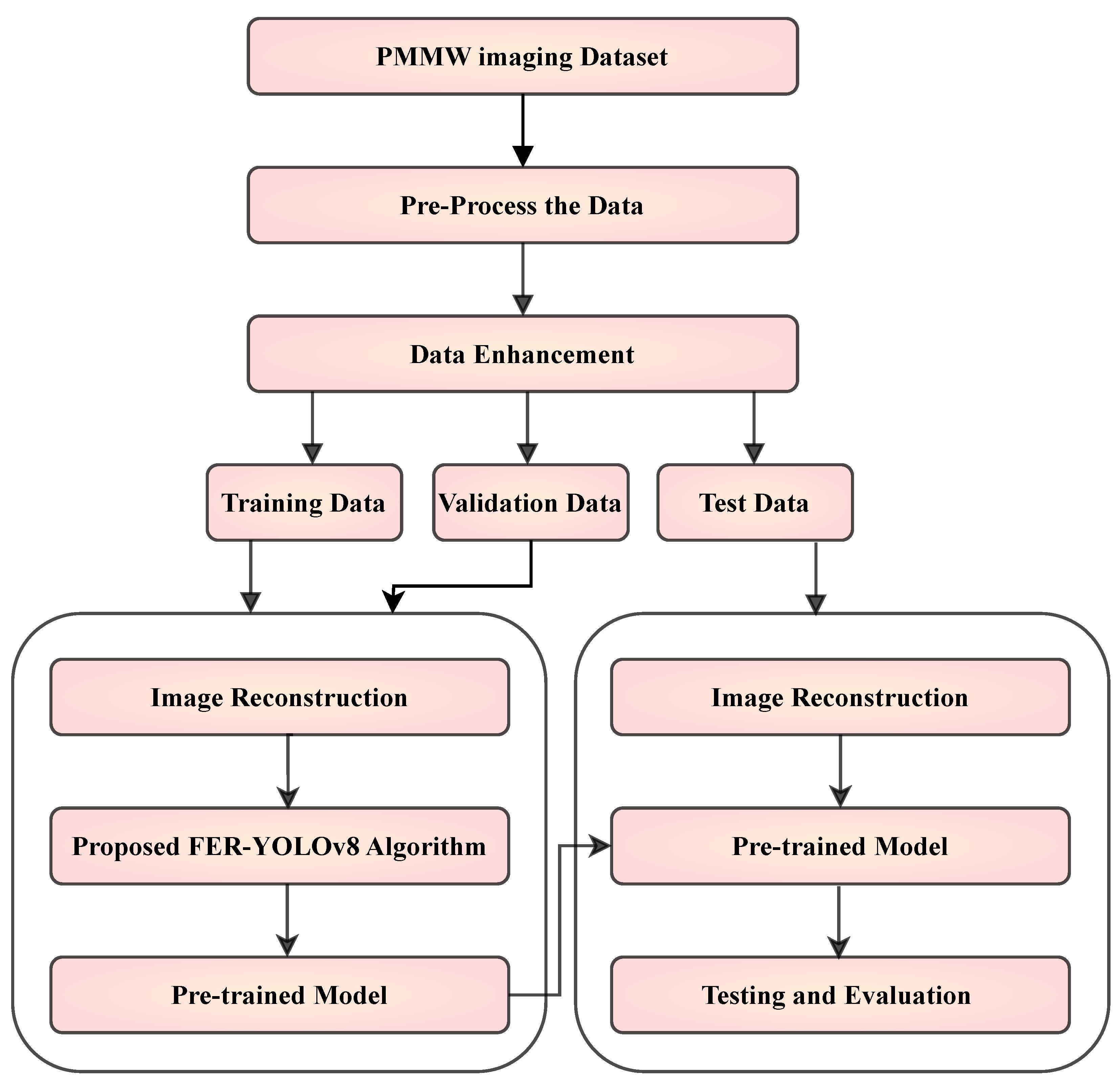
The proposed research framework is shown in Figure 11. The PMMW imaging dataset is collected and an overview of the dataset is mentioned above. The dataset under consideration is then balanced using random sampling during preprocessing. After that, the dataset is enhanced using the α -R BRS approach. The augmented dataset is partitioned into training, validation, and test datasets. The quality of the images in the above three datasets is improved by removing noise and improving SNR values using an adaptive Wiener filter during image reconstruction. The filter-enhanced training data are utilized to train the proposed FER-YOLOv8 algorithm model, while the validation set aids in removing the overfitting and underfitting issues and fine-tuning of the hyperparameters. Then, the evaluation metrics, such as precision, recall, and mean average precision (mAP), of the test data are assessed. The extensive experiments reveal the superiority of the proposed FER-YOLOv8 algorithm over the other SOTA tiny YOLOv3 and YOLOv8 models.

4. System Configuration with Simulation Setup

The proposed study used Python 3.8.0 and the well-known machine learning framework PyTorch 2.0 [69]. The Ultralytics tiny YOLOv3, YOLOv8n, and YOLOv8m repositories were used to train and assess the YOLOv3, YOLOv8n, and YOLOv8m models for detecting concealed weapons, respectively [70]. The Ultralytics YOLOv8m model was then modified to create the proposed FER-YOLOv8 model. The WF was implemented to filter the images using SciPy, an open-source Python (version 1.15.0) toolkit. YOLOv8n and YOLOv8m models were evaluated both on filtered and unfiltered images. Multiple GPU trainings were accelerated in parallel utilizing two Nvidia graphics processing units (GPUs), each with a 10 GB GeForce RTX 3080. Other PC features included anAMD Ryzen processor 7 5800X, a 4.7 GHz CPU, 32 GB of RAM, and a 2 TB hard drive running the Ubuntu operating system. The models were evaluated using a new extended CWD dataset, as mentioned in Section 3.2.2. The new extended CWD dataset contains 6360 grayscale images. All models were trained on 5088 images, validated on 636 images, and then tested on the remaining 636 images.

4.1. Hyperparameter Settings

A list of the hyperparameters that were utilized to fine-tune the tiny YOLOv3, YOLOv8n, and YOLOv8m models is given in Table 1. The two important hyperparameters that notably affect the model’s capacity for generalization and detection accuracy are batch size and epochs. A larger batch size allows the data to be trained using a greater number of samples from the training dataset during a single epoch. A large batch size requires excessive computational resources, such as GPU memory, which makes it difficult to implement detection algorithms in a real-world scenario. Considering the limited computational resources, a batch size of 16 was used in the experiments. To capture the crucial global and local features in an image, the number of training epochs was set to 100. To guarantee impartial comparison, all the models were trained using the same hyperparameters.

4.2. Tiny YOLOv3, YOLOv8n, and YOLOv8m Configurations

The tiny YOLOv3, YOLOv8n, and YOLOv8m models have 82, 225, and 295 layers, respectively. Tiny YOLOv3.pt weights with 25 convolutional layers and 2.6 million (M) parameters were used to train the tiny YOLOv3 model. When compared to tiny YOLOv3, the YOLOv8n and YOLOv8m models utilize 64 and 84 convolutional layers, respectively, and use 3.2 M and 25.9 M parameters. The YOLOv8n.pt and YOLOv8m.pt weights were used to train the YOLOv8n and YOLOv8m models.

4.3. Proposed FER-YOLOv8 Model Configuration

The proposed FER-YOLOv8 model was built on 303 layers, as represented in Figure 12. The number of convolutional layers and parameters supporting model training are also displayed in Figure 12. The YOLOv8m.yaml configuration file was modified to 85 convolutional layers and 2.4 M parameters to train the proposed FER-YOLOv8 model. The ConvModule was changed to the Conv_Reg module, as discussed earlier, by adding a lower-level dropout layer into the ConvModule. Some initial modifications in the backbone network of the suggested FER-YOLOv8 architecture are demonstrated in Table 2.

5. Evaluation Metrics

The effectiveness of the models in this research were evaluated based on quantitative and qualitative analyses. The performance metrics used for the quantitative and qualitative analyses are discussed below.

5.1. Evaluation Metrics for Quantitative Analysis

To confirm the superiority of the proposed FER-YOLOv8 model, the current subsections describe the evaluation metrics which were used to perform a quantitative analysis.

5.1.1. Confusion Matrix

A confusion matrix is utilized to determine each model’s accuracy and reliability on the CWD dataset. The ratio of cases initially labeled as class “i” that were later detected by the model as class “j” is represented by each cell (i, j) in this matrix. The final column in the matrix characterizes false positives, or type-1 mistakes. False positives occur when background items that should be negatives are inappropriately detected as positives. Conversely, type-2 mistakes, also referred to as false negatives, are represented by the bottom row of the matrix. False negatives show instances in which background items are mistakenly categorized as negatives while the above-discussed particular instances belong in the positive category [71].

5.1.2. Precision

The precision metric evaluates the bounding box (bbox) prediction accuracy by calculating the ratio of true positive detections to the total number of true positive and false positive detections [72]. The precision can be mathematically written as in Equation (18):
Precision = T positive T positive + F positive
where Tpositive presents true positive cases and Fpositive indicates false positive cases.

5.1.3. Recall

Recall, which is calculated as the ratio of true positive detections to the total number of true positive and false negative detections, assesses a model’s capacity to accurately predict genuine bbox occurrences. The recall can be mathematically expressed as in Equation (19):
Recall = T positive T positive + F negative
where Tpositive presents true positive cases and Fnegative indicates false negative cases.

5.2. Qualitative Analysis

Qualitative analysis particularly depicts the robustness of a model’s performance on different confidence intervals and intersection-over-union (IoU) threshold values. The qualitative analysis involves a visual representation of the model’s CWD quality.

6. Simulation Results and Discussion

The current section provides an in-depth quantitative and qualitative analysis of the assessment results of the recently trained models such as tiny YOLOv3, YOLOv8n, YOLOv8m, YOLOv8n with a Wiener filter (YOLOv8n-WF), YOLOv8m with a Wiener filter (YOLOv8m-WF), and the proposed FER-YOLOv8 model.

6.1. Qualitative Assessments

The proposed FER-YOLOv8 model is compared with the tiny YOLOv3, YOLOv8n, YOLOv8m, YOLOv8n-WF, and YOLOv8m-WF models to explore the performance of the aforementioned models in CWD. Quantitative evaluations are used to reveal the validity of the proposed FER-YOLOv8 model for CWD, as described in the coming subsections.

6.1.1. Error Evaluation

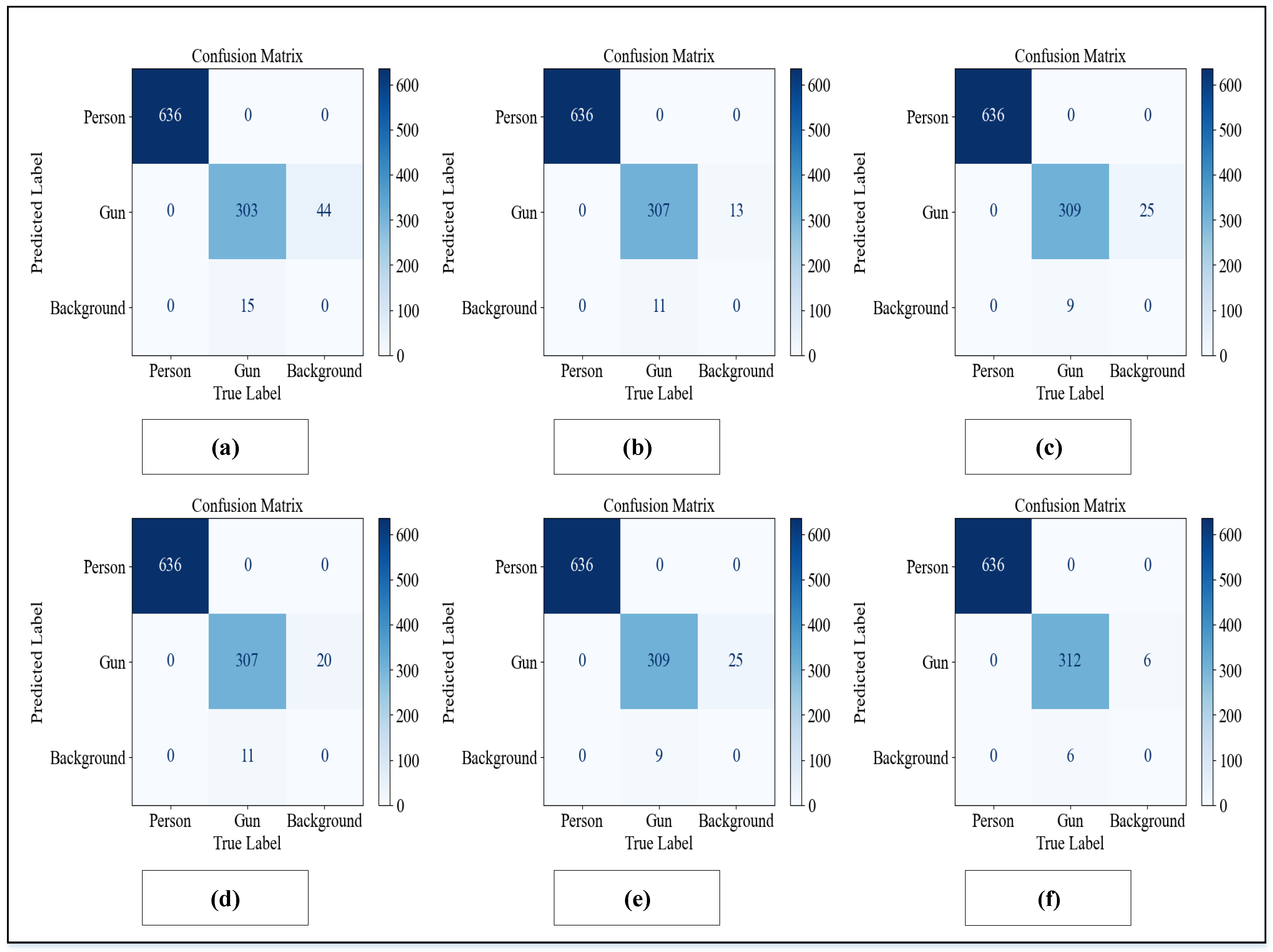
The precision and error of the models with a 0.25 confidence level and a 0.50 IoU threshold on the test dataset, which encompasses 636 images, are shown in Figure 13a–f. The test data consist of 318 positive images. The performance of the tiny YOLOv3, YOLOv8n, YOLOv8m, YOLOv8n-WF, YOLOv8m-WF, and proposed FER-YOLOv8 models is remarkable in detecting concealed weapons. On the other hand, a greater value of the “person” class along the diagonal relative to the other classes indicates that the model is quite good at recognizing the “person” class. The type-1 error deduced from Figure 13a–h for the “gun” class for the tiny YOLOv3, YOLOv8n, YOLOv8m, YOLOv8n-WF, YOLOv8m-WF, and proposed FER-YOLOv8 models is 13%, 4%, 7.8%, 6.2%, 2.5%, and 1.8%, respectively. Moreover, the type-2 error for the “gun” class for the tiny YOLOv3, YOLOv8n, YOLOv8m, YOLOv8n-WF, YOLOv8m-Wiener filter, and proposed FER-YOLOv8 models is 4.7%, 3.4%, 3.1%, 3.4%, 3.7%, and 1.8%, respectively.
The type-1 and type-2 errors in tiny YOLOv3 are higher than the variants of YOLOv8, such as YOLOv8n, YOLOv8m, YOLOv8n-WF, YOLOv8m-WF, and the proposed FER-YOLOv8 models, as delineated in Figure 13a–f. YOLOv8 models take advantage of PAN-FPN modules, which refine the extracted features related to each class at various scales in the neck and backbone sections of YOLOv8 variants. Ultimately, the YOLOv8 models are more capable of differentiating the classes based on the distinguished features captured from each class as compared to the tiny YOLOv3 model. Hence, the type-1 and type-2 errors diminish significantly in the YOLOv8 architectures as compared to the tiny YOLOv3 architecture. Moreover, the YOLOv8m architecture improves the type-1 and type-2 errors as compared to the YOLOv8n architecture due to a higher number of convolutional layers in the YOLOv8m architecture.
The proposed FER-YOLOv8 architecture extends the backbone network by introducing the FER module and dropout layers in the CSP module to capture more relevant features from the low-contextual images captured from the PMMW imaging dataset. The newly introduced FER module uses a convolutional layer of 1 × 1 filter size, which captures the significant local features while avoiding the loss of contextual information and the size of an image. The other reason to implement the FER module in the beginning of the backbone network in the proposed FER-YOLOv8 is to ensure the extrication of specific local features, which are related to pose and view-point variations. Hence, the proposed FER-YOLOv8 architecture improves the capability of feature extraction as compared to the above-mentioned tiny YOLOv3 and YOLOv8 variants, which drastically reduces the type-1 and type-2 errors.

6.1.2. Precision Assessment

In the application of CWD, Table 3 shows the precision performance of the tiny YOLOv3 YOLOv8n, YOLOv8m, YOLOv8n-WF, YOLOv8m-WF, and recommended FER-YOLOv8 models. Table 3 presents the precision evaluation of the previously stated models, both overall and per class. The suggested FER-YOLOv8 reaches a precision value of up to 0.995 for the whole set of test images. Comparably, the gun class’s precision is 0.981, significantly greater than that of the other stated models. In a similar vein, the YOLOv8m-WF model’s performance is defined as follows: for the gun class, the model’s precision value is up to 0.925. Similarly, the YOLOv8m model’s performance for the gun class is slightly less than the YOLOv8m-WF model. The macro-averaging precision values are also mentioned in Table 3. The macro-averaging precision values also suggest that the proposed FER-YOLOv8 model outperforms the other models.
The precision value merely relies on the true positive and false positive detections, as described in Equation (18). The proposed FER-YOLOv8 architecture outperforms the other comparable tiny YOLOv3 and YOLOv8 architectures by decreasing the false positive rate due to the enormous feature extraction capability offered by the FER module. Moreover, the extension of the dropout layer in the modified Conv_Reg module combats overfitting, which also improves the generalization capability of the proposed FER-YOLOv8 architecture as compared to the other models. Thus, the precision of the suggested FER-YOLOv8 architecture on the gun class increases to 98.1%, which is high compared to the other YOLOv3 model and YOLOv8 variants, as depicted in Table 3.

6.1.3. Recall Assessment

Table 4 demonstrates the recall attainment of the tiny YOLOv3, YOLOv8n, YOLOv8m, YOLOv8n-WF, YOLOv8m-WF, and recommended FER-YOLOv8 models for the CWD system. Table 4 depicts the recall evaluation of the above-mentioned models, both overall and per class. The suggested FER-YOLOv8 reaches a recall value of up to 0.993 for the whole set of test images. Comparably, the gun class’s recall is 0.981, appreciably greater than that of the other models. On a similar evaluation metric, the YOLOv8m-WF model’s performance is defined as follows: for the gun class, the model’s recall value is up to 0.972. Similarly, the YOLOv8m model’s performance for the gun class is also the same as the performance of YOLOv8m-WF model. The macro-averaging recall values are also stated in Table 4. The macro-averaging recall values also suggest that the proposed FER-YOLOv8 model outclasses the other models.
The recall value simply depends on the true positive and false negative detections, as described in Equation (19). The proposed FER-YOLOv8 architecture outperforms the other competitor models, such as tiny YOLOv3 and YOLOv8 architectures, by decreasing the false negative rate and improving the true positive detections. Again, the enhanced feature extraction capability provided by the pointwise convolution in the FER module in the backbone network of the recommended FER-YOLOv8 architecture improves the recall value of the CWD system. Moreover, the extension of the dropout layer in the modified Conv_Reg module combats overfitting, which also improves the generalization capability of the proposed FER-YOLOv8 architecture as compared to the other models. Thus, the recall of the gun class by the suggested FER-YOLOv8 architecture increases to 98.1%, which is extraordinary compared to the tiny YOLOv3 model and YOLOv8 variants, as mentioned in Table 4.

6.1.4. Mean Average Precision (mAP ⇒ 0.5)

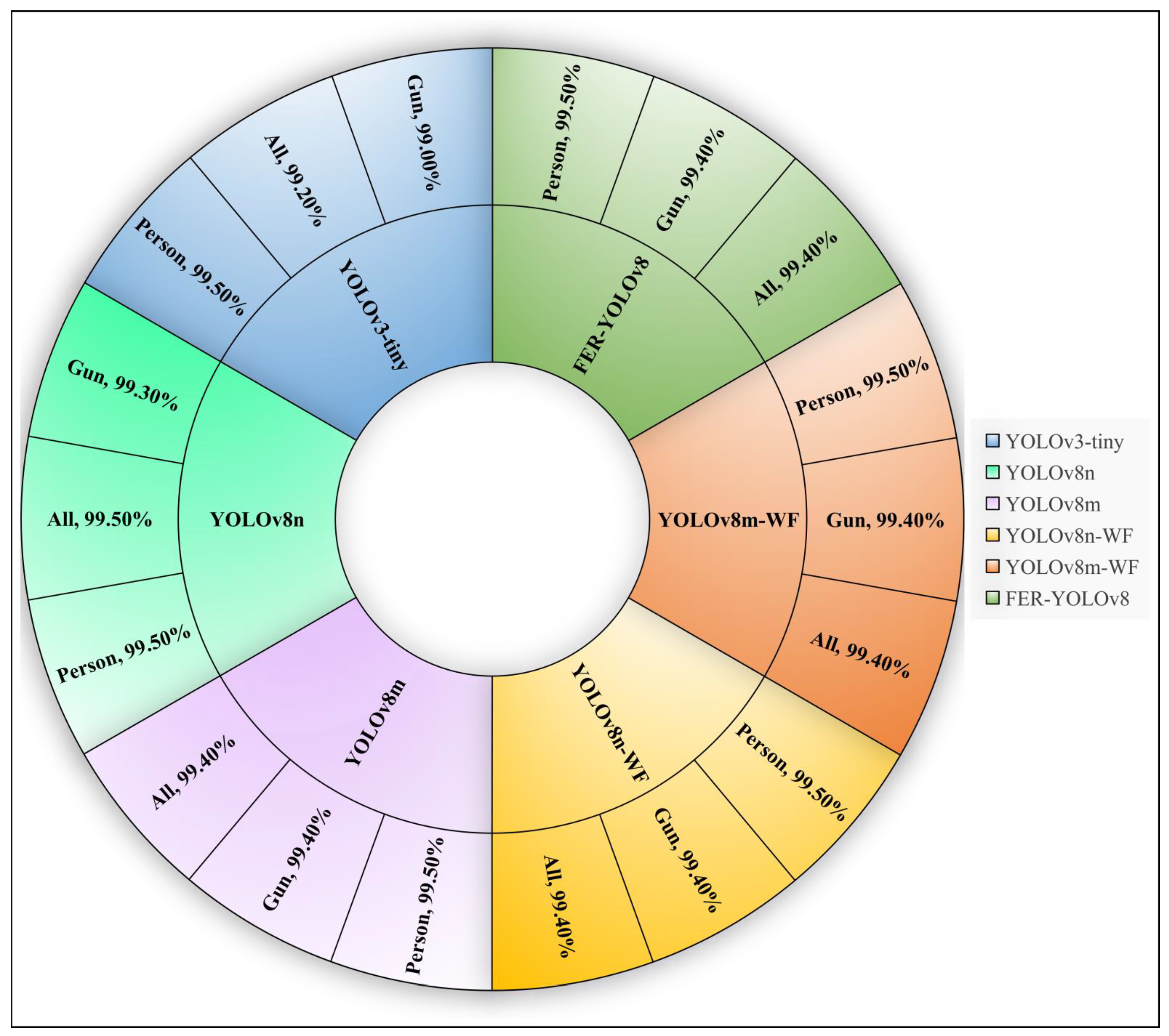
For the test dataset of the CWD system mentioned above, Figure 14 delineates the assessment of mAP 0.5 scores for the following algorithms: the proposed FER-YOLOv8, tiny YOLOv3, YOLOv8n, YOLOv8m, YOLOv8n-WF, and YOLOv8m-WF. The suggested FER-YOLOv8 model reaches an mAP 0.5 value of up to 0.994 for the whole set of test images. In a similar vein, the mAP 0.5 for the “person” class achieves 0.995. Similarly, the SOTA tiny YOLOv3 model, whose mAP 0.5 value for the “gun” class reaches up to 0.99, performs approximately the same as the suggested FER-YOLOv8 model, which obtains an mAP 0.5 value for the “gun” class up to 0.994. Likewise, the YOLOv8m-WF model’s performance may be explained as follows: For the total test images, the YOLOv8m-WF model reaches an mAP 0.5 value of up to 0.994. Additionally, Figure 14 also shows the mAP 0.5 values for the other models.
The mAP 0.5 value of the proposed FER-YOLOv8 model extends up to 99.4% when the IoU threshold is set to 0.50 . The mAP 0.5 value of the gun class attained by the proposed architecture is 99.4%, which is greater than the tiny YOLOv3 architecture, as shown in Figure 14 because of the advanced backbone, neck, and head sections in the proposed FER-YOLOv8 architecture. However, the mAP 0.5 value of the recommended FER-YOLOv8 architecture and the other variants of the YOLOv8 models are similar because the models already achieved optimal mAP 0.5 values at the 0.50 IoU threshold.

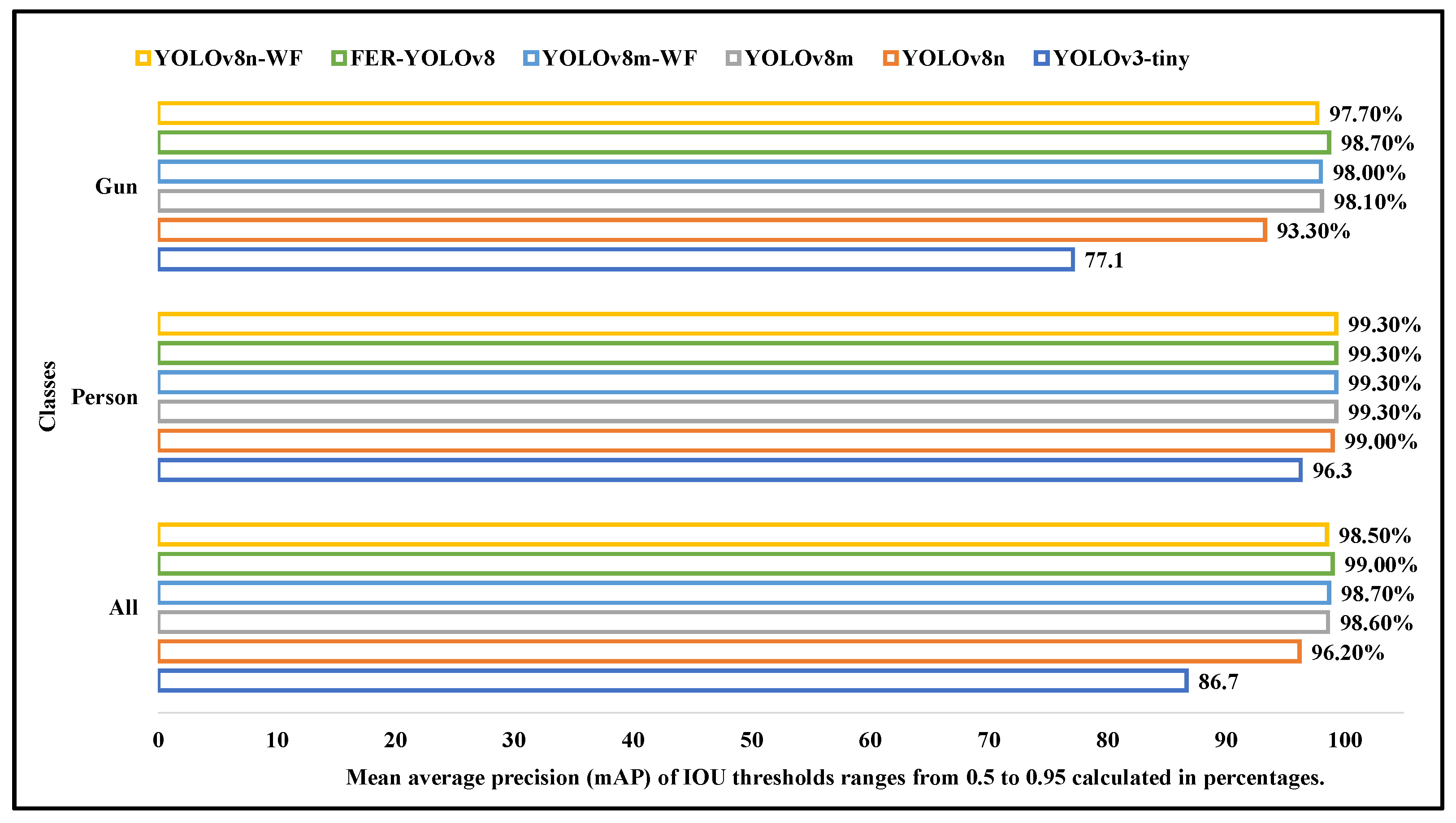
6.1.5. Mean Average Precision (mAP ⇒ 0.5:0.95)

Mean average precision with a range of IoU thresholds of 0.5 to 0.95 ( mAP 0.5:0.95) is a more stringent criteria to measure the performance of detection phenomena. Aimed at the test dataset of the CWD system mentioned above, Figure 15 presents the mAP 0.5:0.95 scores for the following algorithms: the proposed FER-YOLOv8, tiny YOLOv3, YOLOv8n, YOLOv8m, YOLOv8n-WF, and YOLOv8m-WF. The suggested FER-YOLOv8 model attains an mAP 0.5:0.95 value of up to 0.99 for the whole set of test images. In a similar vein, the mAP 0.5:0.95 achieved for the “gun” class is 0.987. Similarly, the SOTA tiny YOLOv3 model, whose mAP 0.5:0.95 value for the “gun” class reaches up to 0.771, performs worse than the suggested FER-YOLOv8 model, which obtains an mAP 0.5:0.95 value for the “gun” class up to 0.987. Moreover, the SOTA tiny YOLOv3 model also performs worse than the YOLOv8 variants, especially the suggested FER-YOLOv8 algorithm, because the SOTA tiny YOLOv3 algorithm has limited capability for extraction of local and global features in an image. Likewise, the YOLOv8m-WF model’s performance may be explained as follows: For the total test images, the YOLOv8m-WF model reaches an mAP 0.5:0.95 value of up to 0.987. Additionally, Figure 15 also illustrates the mAP 0.5:0.95 values for the other models.
The suggested FER-YOLOv8 model achieves an mAP 0.5:0.95 value of up to 0.987 for the gun class, which is greater than the mAP 0.5:0.95 value of the SOTA tiny YOLOv3 model, as depicted in Figure 15. To improve the CWD mechanism’s stability, a pointwise convolution in the beginning of the backbone network aims to capture more specific features related to pose variations from low-resolution and noisy images. Moreover, the adequate number of dropout layers in Conv_Reg modules minimizes the number of parameters, allowing the model to become more resistant to overfitting. The implementation of 1 × 1 convolution filters and dropout layers with an optimal loss function CIoU enhances the superiority of the proposed architecture over other models in terms of robust detection of hidden weapons against more complicated mAP criteria when the IoU threshold ranges from 0.5 to 0.95.

6.1.6. Comparison of F1-Confidence Curves

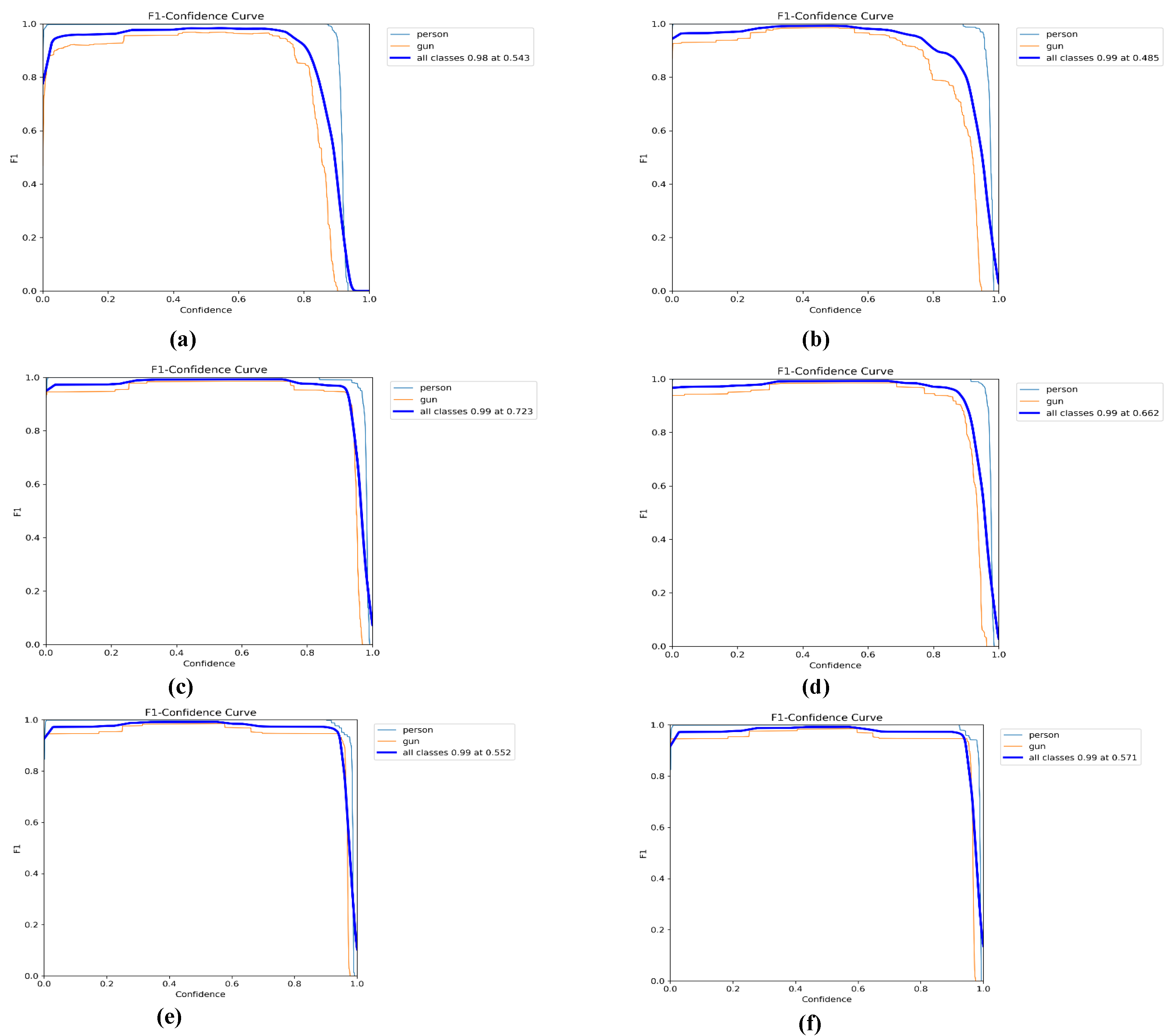
Figure 16 illustrates the attainment of the F1-score with respect to the confidence values. In Figure 16a, the F1-score achieves its highest value of 0.98 when the optimal confidence value is configured at 0.543 for all classes by the tiny YOLOv3 algorithm. In contrast, the highest F1-score achieved by the suggested FER-YOLOv8 model and the presented research framework is 0.99 at the confidence value of 0.571, as shown in Figure 16f. Significantly, the “gun” class exhibits an extraordinary improvement in obtaining the optimal F1-score quickly after the confidence value exceeds 0.1. The performance of other models in terms of F1-scores is also shown in Figure 16b–e.
The model’s assurance in detecting the real hidden objects is determined by the confidence score. The stability in correctly detecting the concealed object is affirmed by the model maintaining a better F1-score when compared to higher confidence values. The F1-scores of the gun class versus the confidence scores are shown in Figure 16 as an orange graph. When the SOTA tiny YOLOv3 algorithm is tested for a confidence value of more than 0.8, the F1-score of the SOTA tiny YOLOv3 algorithm abruptly decreases to the minimal value, as shown in Figure 16a. The mapping of the F1-scores versus the confidence values corresponding to the gun class shows a lower capability to detect forbidden objects efficiently under strict criteria. Similarly, an unstable pattern in the peak variations of the F1-score is observed for lower confidence values, i.e., 0. The other YOLOv8 variants, such as YOLOv8n, YOLOv8m, YOLOv8n-WF, and YOLOv8m-WF, show better detection capability and stability in operating the concealed detection process, as shown in Figure 16b–e. The F1-curves of the recommended FER-YOLOv8 algorithm associated with the gun class, person class, and for all classes are visualized in Figure 16f. The F1-curves of the proposed FER-YOLOv8 algorithm cover the wider region of the graph for not only the person class but also for the gun class, which ensures the better detection capability of both the person and gun classes. Moreover, the peak variations of the F1-curve also confirm the stability in the detection process as compared to the other tiny YOLOv3 model and YOLOv8 variants.

6.1.7. Comparison of Precision–Recall (PR) Curve

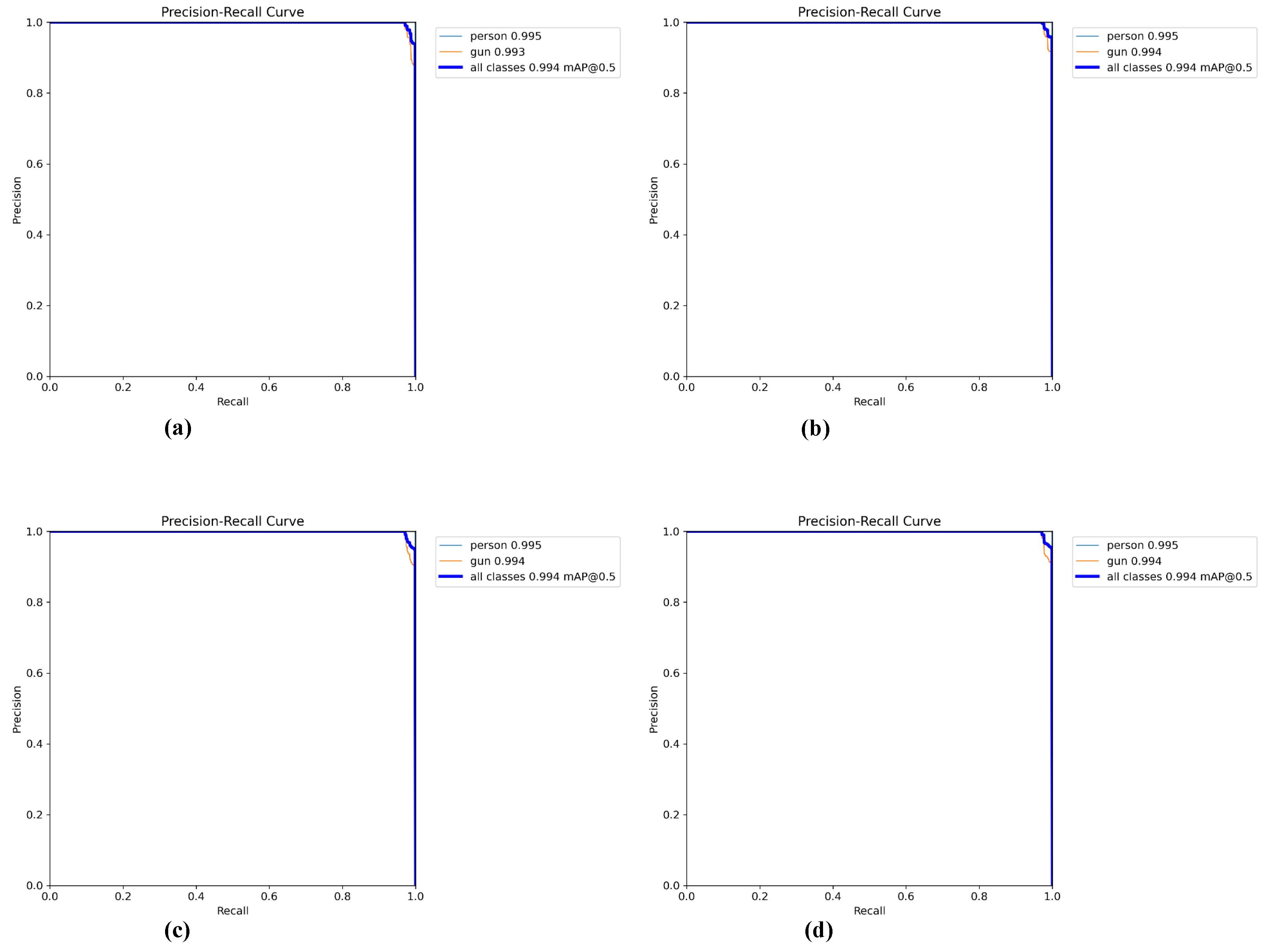
The evaluation outcomes utilizing the PR curves for the proposed FER-YOLOv8 algorithm and SOTA tiny YOLOv3 algorithm are shown in Figure 17a,b. The PR curve effectively balances recall and precision by altering the confidence value to optimize the mAP value. A 0.5 IoU cutoff was applied to every model. A threshold of 0.5 IoU was used to evaluate all models. The top mAP for the proposed FER-YOLOv8 model is 99.4% for all classes. Specifically, the suggested framework achieves 99.4% for the gun class and 99.5% for the person class, as indicated in Figure 17b. Contrary to the suggested algorithm and framework, the SOTA tiny YOLOv3 algorithm obtains an mAP of 99.2% for all classes and 99.0% for the gun class, which is lower compared to the proposed algorithm.
The PR curves for other models, such as YOLOv8n, YOLOv8m, YOLOv8n-WF, and YOLOv8m-WF, are also shown in Figure 18a–d. The area under the PR curve of the presented FER-YOLOv8 model is larger, as shown in Figure 17a. While the area under the PR curve of the SOTA tiny YOLOv3 model is smaller, as represented in Figure 17b. The larger area under the PR curve corresponds to good model performance and a good balance between high precision and high recall. Hence, the proposed architecture outperforms the tiny YOLOv3 model and YOLOv8 variants in terms of maintaining high precision and high recall for all classes in the CWD system.

6.1.8. Computational Complexity

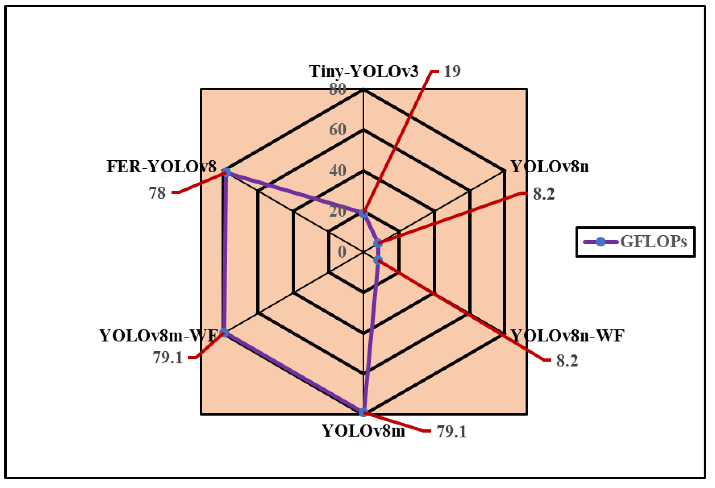
The computational efficiency of the DL algorithms and high-performance computers is usually measured in giga floating point operations per second (GFLOPs) for real-time utilization. The algorithm, which has high GFLOPs, requires GPUs for the efficient detection of concealed weapons. For instance, the tiny YOLOv3 model has a computational complexity of 19.0 GFLOPs to detect the concealed weapons, as shown in Figure 19. Hence, the tiny YOLOv3 model requires fewer computational resources than the other models. However, the tiny YOLOv3 model fails to detect concealed guns in many cases, as the tiny YOLOv3 model achieves a precision of up to 87.3%. Therefore, the unconvincing performance of the tiny YOLOv3 model again poses a limitation to its use in a real-time concealed weapon detection system. The complete quantitative analysis of the tiny YOLOv3 model is presented in Table 3 and Table 4 of the manuscript.
Moreover, lightweight models are usually incapable of extracting sufficient contextual information from grayscale noise-perturbed images. Whereas, the images captured by the PMMW imaging systems suffer intensely from high noise and low resolution, which makes lightweight models impractical for the task of the detection of small concealed objects.
On the other hand, the YOLOv8m-WF model requires 79.1 GFLOPs to achieve a precision of up to 92.9% while detecting the hidden guns. Hence, the YOLOv8m-WF model surpasses the tiny YOLOv3 model on account of increased model complexity. This paper successfully proposes a new BWFER-YOLOv8 model, which surpasses the YOLOv8m-WF model by achieving a precision of 98.1% while reducing the GFLOPs to 78.0. The proposed BWFER-YOLOv8 model also improves the other evaluation metrics, as discussed above, without increasing the GFLOPs compared to YOLOv8-WF. The extensive experiments demonstrate that the accuracy of concealed weapon detection systems can be compromised by using low-complexity models. The proposed work recommends that a trade-off between the complexity of the model and the efficiency of the concealed weapon detection system is the best solution to address life-threatening scenarios in real-time surveillance systems.

6.2. Qualitative Analysis

To further validate the efficiency of the proposed FER-YOLOv8 algorithm and proposed research framework on a PMMW imaging dataset, a qualitative analysis was performed to prove the supremacy of the proposed algorithm.
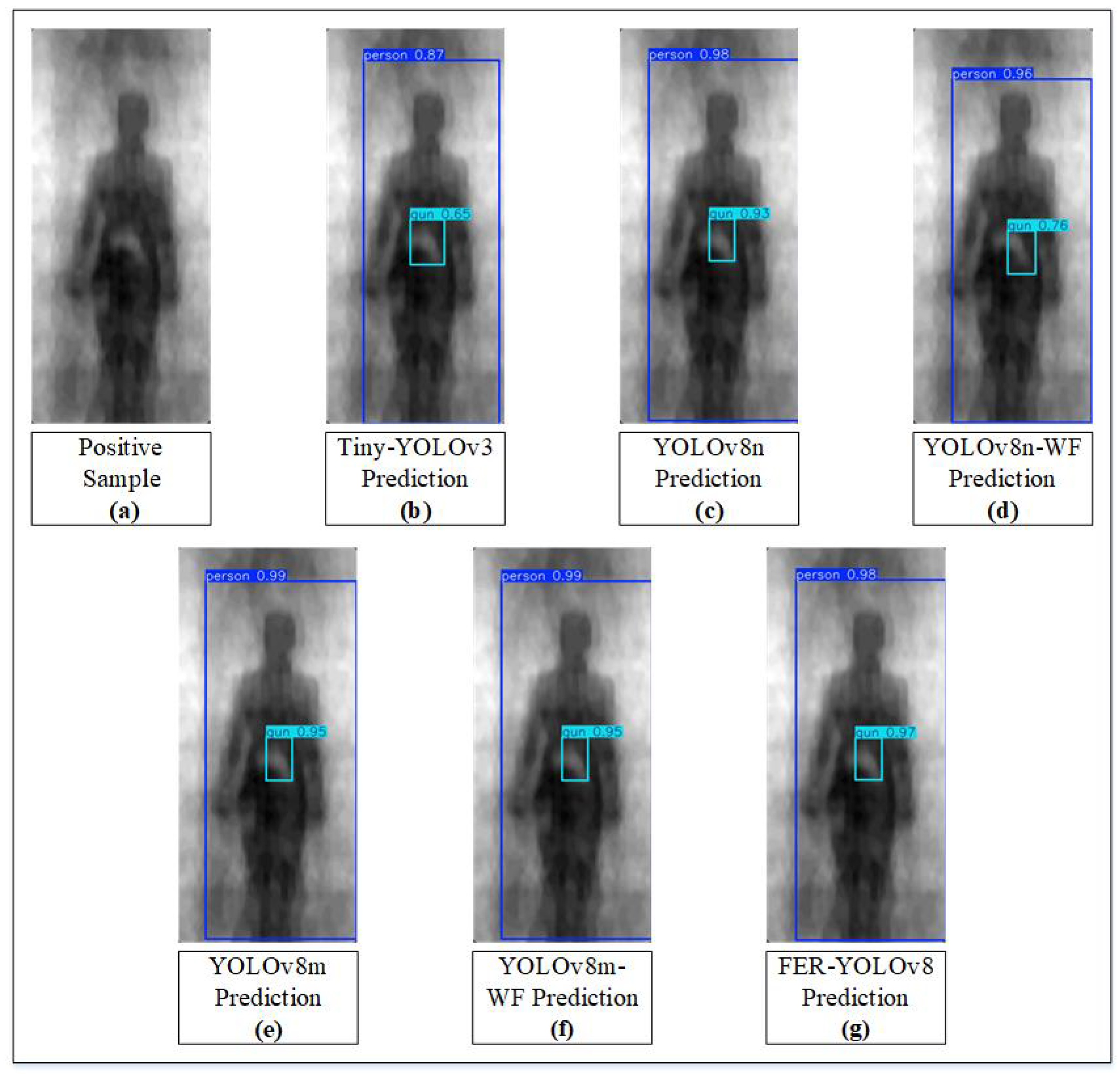
For a deep qualitative comparison between the proposed models and the other models described above, consider the true positive criteria in which the positive sample is selected randomly from the ground truth and all the above-mentioned trained models detect the person and gun class accurately, as shown in Figure 20.
The certainty of detecting the gun in a particular positive sample using the SOTA tiny YOLOv3 algorithm is 0.65. The certainty of detecting the gun in a particular positive sample using the YOLOv8m-WF algorithm is 0.95. However, the prediction certainty of the gun using the proposed FER-YOLOv8 algorithm is 0.97, which is higher than the SOTA tiny YOLOv3 algorithm and other YOLOv8 variants. The connected regions in the detection of the person class in YOLOv8n-WF are less than for the other models. However, the prediction score in the YOLOv8n-WF model for the person class and the gun class is relatively lower than the YOLOv8 variants, which makes the YOLOv8n-WF model difficult to use. According to the above-presented analysis, when the criteria are based on the detection scores of the person and gun classes, the recommended FER-YOLOv8 model performs better than the other models.
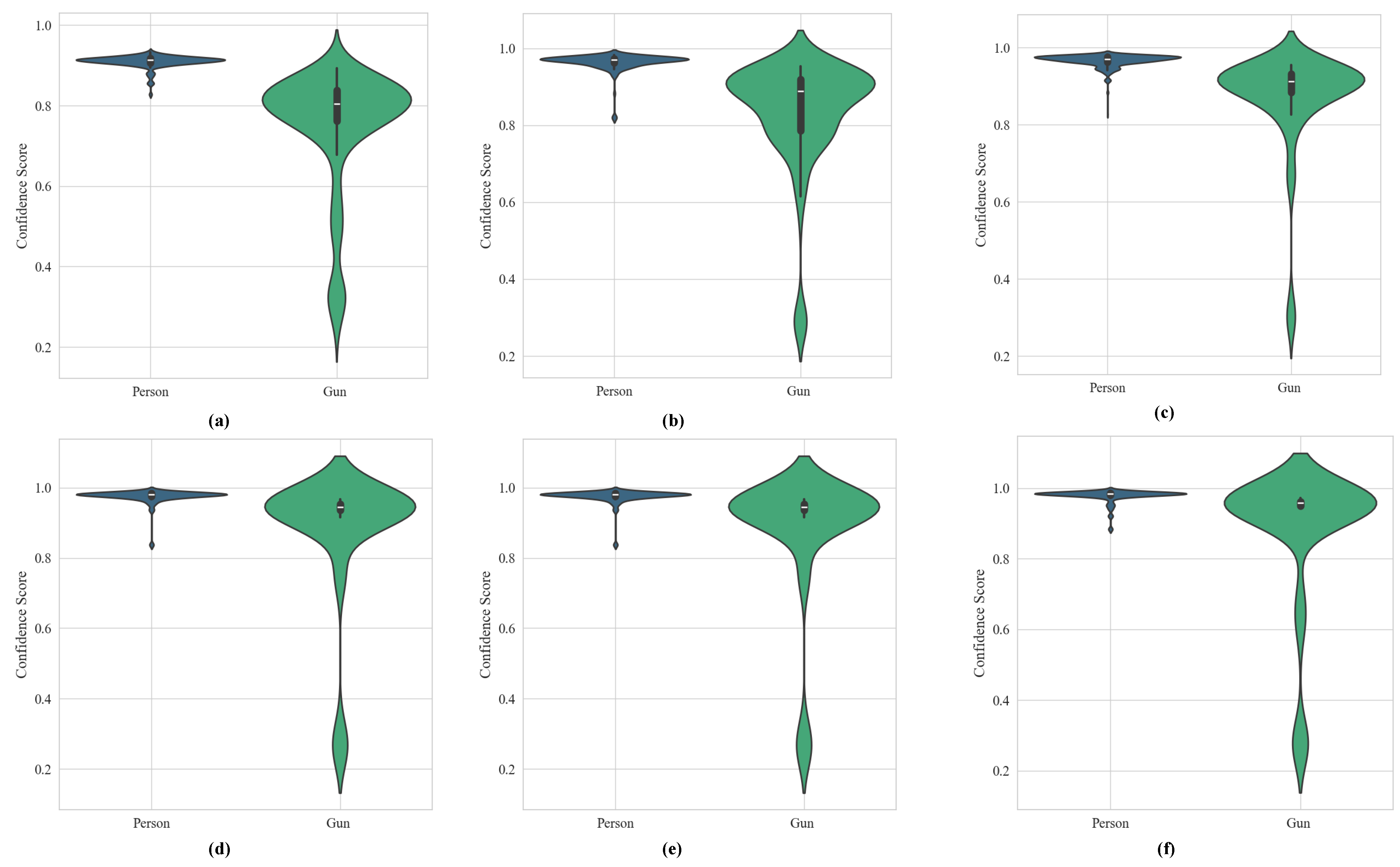
To ensure consistency and robustness in the accurate detection of concealed weapons with higher certainty, a comparison of the distribution of the confidence scores in detecting the gun and person classes for the above-mentioned trained models was compiled and is illustrated in Figure 21. The white thin line in each violin plot represents the median of the confidence scores. The median value of the confidence scores of the SOTA tiny YOLOv3 algorithm is 0.80 for the gun class. The minimum and maximum confidence scores of the tiny YOLOv3 algorithm observed on the test dataset are 0.27 and 0.89, respectively. The median values of the confidence scores of the YOLOv8n, YOLOv8n-WF, YOLOv8m, and YOLOv8m-WF models are 0.88, 0.91, 0.94, and 0.94, respectively. The higher median values of the YOLOv8 variants divulge that the reliability in detecting a gun accurately in each test image inclines towards a higher quantile region as compared to the tiny YOLOv3 algorithm.
The above-discussed performance can also be visualized by the distribution shape of the confidence scores, as represented in Figure 21. The widths of the upper lobes of the violin plots for the YOLOv8m and YOLOv8m-WF models are wider than the widths of the upper lobes of the tiny YOLOv3 and YOLOv8n models, which indicates that the density of the confidence score values for the YOLOv8m and YOLOv8m-WF models is higher in the third quantile region. Hence, the YOLOv8 variants experience more robustness and consistency in the detection of concealed objects than the tiny YOLOv3 algorithm. Similarly the minimum and maximum confidence scores of the YOLOv8m-WF algorithm are 0.27 and 0.97. The median value of the confidence scores of the proposed FER-YOLOv8 algorithm is 0.96 for the gun class, which is higher than the above-discussed models. The minimum and maximum confidence scores of the tiny YOLOv3 algorithm observed on the test dataset are 0.27 and 0.89. Therefore, the extensive experiments show that the proposed FER-YOLOv8 algorithm is more reliable for CWD systems.
The quality of the trained models can be improved by reducing the false positive rate in the detection of concealed weapons such as small guns, etc. The proposed research framework significantly reduces the false positive detection rate, by 1.8%, as compared to the SOTA tiny-YOLOv3 algorithm, which has a false positive detection rate of 13%. Figure 22 illustrates a comparison of the aforementioned various trained models on one of the sample images without a gun. All the models except YOLOv8n-WF and the proposed FER-YOLOv8 detect the gun erroneously in the particular sample. However, the confusion matrix suggests that the proposed research framework accomplishes remarkable performance as compared to YOLOv8n-WF by reducing the false positive detection rate from 6.2% to 1.8% on the whole test dataset.
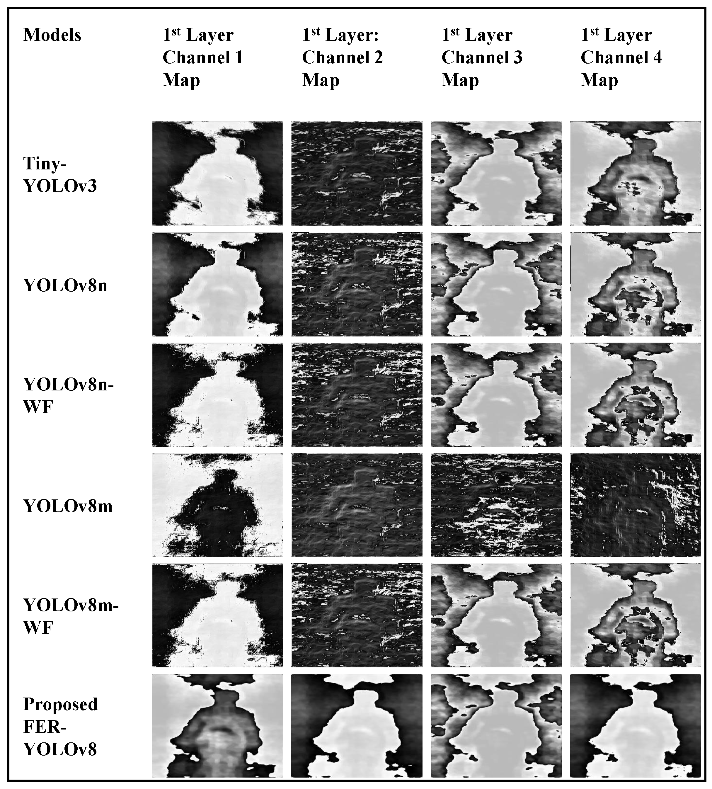
The distinguished performance of the FER-YOLOv8 algorithm is due to the convincing feature extraction capability of the 1 × 1 convolution filter in the FER module, which is implemented at the beginning of the backbone network as a first convolutional layer in the proposed FER-YOLOv8 algorithm. A comparison of the feature maps of the first layer of various models under consideration is shown in Figure 23. When contrasted channel-wise with the feature maps of the other models for concealed weapon detection, the FER module’s 1 × 1 convolution filter has improved the potential of object-to-background distinction, making the recommended algorithm suitable for real-world scenarios.

7. Conclusions

In this paper, the authors presented BWFER-YOLOv8, a new enhanced tri-cascaded framework for a small-size CWD, by using images captured by PMMWI sensors. The proposed framework integrated a novel α -R BRS method, adaptive WF, and a new FER-YOLOv8 architecture to confront the challenges posed by noise, a low SNR, and nonuniform illumination simultaneously. A novel α -R BRS method was deployed, which enhanced the PMMWI dataset to capture highly complex features during training of the model. Adaptive WF effectively alleviated the low SNR and de-noised the PMMW images convincingly, which resulted in the enhanced quality of the reconstructed images. A newly developed FER-YOLOv8 architecture employed FER and Conv_Reg modules in the backbone network. Hence, the proposed framework significantly extracted the local and global features. The recommended framework achieved a precision of 98.1% in detecting the guns, which is relatively higher than the SOTA tiny YOLOv3 and other YOLOv8 models. The SOTA tiny YOLOv3 obtained a precision of 87.3% in detecting the guns in the PMMW images. The macro-averaging precision for the detection of all the classes was also improved by deploying the recommended framework. Similarly, other important evaluation metrics, such as recall and mAP ⇒ 0.5:0.95, also significantly improved to the desired extent. A qualitative analysis also suggested that the recommended framework and architecture boosted the quality of the COD process by adequately extracting highly complex features as compared to the SOTA tiny YOLOv3 and YOLOv8 models.
As future work, the proposed framework will be deployed in a practical scenario using a real-time PMMW imaging system. The other main technologies used to procure the CWD image datasets are AMMWI and FMCW radar systems. The above-mentioned technologies require different specifications and environmental conditions to capture the CWD datasets. Therefore, the CWD image datasets obtained from the AMMWI and FMCW radar systems are comparatively different from the PMMWI datasets. Furthermore, the proposed framework will be implemented on the publicly available AMMWI and FMCW radar CWD datasets to address the issues encountered by the AMMWI and FMCW CWD systems.

Author Contributions

Conceptualization, K.I., I.K. and E.A.A.; methodology, K.I., I.K. and S.F.A.; software, K.I., I.K. and S.F.A.; validation, K.I., I.K. and E.A.A.; formal analysis, I.K., S.F.A. and E.A.A.; investigation, K.I., I.K. and E.A.A.; resources, K.I., A.H. and F.A.B.; data curation, K.I., I.K. and S.F.A.; writing—original draft preparation, K.I., I.K. and A.H.; writing—review and editing, K.I., I.K., S.F.A. and E.A.A.; visualization, K.I., I.K. and F.A.B.; supervision, I.K., S.F.A. and E.A.A.; project administration, K.I., I.K., A.H. and F.A.B.; funding acquisition, K.I., I.K., A.H. and F.A.B. All authors have read and agreed to the published version of the manuscript.

Funding

This research received no external funding.

Institutional Review Board Statement

Not applicable.

Informed Consent Statement

Not applicable.

Data Availability Statement

The dataset can be downloaded from https://www.mdpi.com/1424-8220/20/6/1678/s1 (accessed on 20 February 2024). The code is available at https://github.com/khalidijaz/Concealed-Object-Detection (accessed on 5 January 2024).

Conflicts of Interest

The authors declare no conflicts of interest.

References

  1. Huang, P.; Wei, R.; Su, Y.; Tan, W. Swin-YOLO for concealed object detection in millimeter wave images. Appl. Sci. 2023, 13, 9793. [Google Scholar] [CrossRef]
  2. Accardo, J.; Chaudhry, M.A. Radiation exposure and privacy concerns surrounding full-body scanners in airports. J. Radiat. Res. Appl. Sci. 2014, 7, 198–200. [Google Scholar] [CrossRef]
  3. Yang, X.; Wei, Z.; Wang, N.; Song, B.; Gao, X. A novel deformable body partition model for MMW suspicious object detection and dynamic tracking. Signal Process. 2020, 174, 107627. [Google Scholar] [CrossRef]
  4. Golenkov, A.; Shevchik-Shekera, A.; Kovbasa, M.Y.; Lysiuk, I.; Vuichyk, M.; Korinets, S.; Bunchuk, S.; Dukhnin, S.; Reva, V.; Sizov, F. THz linear array scanner in application to the real-time imaging and convolutional neural network recognition. Semicond. Phys. Quantum Electron. Optoelectron. 2021, 24, 90–99. [Google Scholar] [CrossRef]
  5. Global Terrorism Index 2024 Key Findings. Institute for Economics and Peace. Available online: https://www.visionofhumanity.org/7-key-findings-from-the-global-terrorism-index-2024 (accessed on 29 February 2024).
  6. Chen, H.M.; Lee, S.; Rao, R.M.; Slamani, M.A.; Varshney, P.K. Imaging for concealed weapon detection: A tutorial overview of development in imaging sensors and processing. IEEE Signal Process. Mag. 2005, 22, 52–61. [Google Scholar] [CrossRef]
  7. Agurto, A.; Li, Y.; Tian, G.Y.; Bowring, N.; Lockwood, S. A review of concealed weapon detection and research in perspective. In Proceedings of the 2007 IEEE International Conference on Networking, Sensing and Control, London, UK, 15–17 April 2007; pp. 443–448. [Google Scholar]
  8. Wang, L.M.; Li, N.; Ren, C.P.; Peng, Z.Y.; Lu, H.Z.; Li, D.; Wu, X.Y.; Zhou, Z.X.; Deng, J.Y.; Zheng, Z.H.; et al. Sterility of Aedes albopictus by X-ray Irradiation as an Alternative to γ-ray Irradiation for the Sterile Insect Technique. Pathogens 2023, 12, 102. [Google Scholar] [CrossRef]
  9. Riz à Porta, R.; Sterchi, Y.; Schwaninger, A. How realistic is threat image projection for x-ray baggage screening? Sensors 2022, 22, 2220. [Google Scholar] [CrossRef]
  10. Velayudhan, D.; Hassan, T.; Ahmed, A.H.; Damiani, E.; Werghi, N. Baggage threat recognition using deep low-rank broad learning detector. In Proceedings of the 2022 IEEE 21st Mediterranean Electrotechnical Conference (MELECON), Palermo, Italy, 14–16 June 2022; pp. 966–971. [Google Scholar]
  11. Kovbasa, M.; Golenkov, A.; Sizov, F. Neural network application to the postal terahertz scanner for automated detection of concealed items. In Proceedings of the 2020 IEEE Ukrainian Microwave Week (UkrMW), Kharkiv, Ukraine, 21–25 September 2020; pp. 870–873. [Google Scholar]
  12. Liu, L.; Ouyang, W.; Wang, X.; Fieguth, P.; Chen, J.; Liu, X.; Pietikäinen, M. Deep learning for generic object detection: A survey. Int. J. Comput. Vis. 2020, 128, 261–318. [Google Scholar] [CrossRef]
  13. Cuadrado-Calle, D.; Piironen, P.; Ayllon, N. Solid-state diode technology for millimeter and submillimeter-wave remote sensing applications: Current status and future trends. IEEE Microw. Mag. 2022, 23, 44–56. [Google Scholar] [CrossRef]
  14. Cheng, Y.; Qiao, L.; Zhu, D.; Wang, Y.; Zhao, Z. Passive polarimetric imaging of millimeter and terahertz waves for personnel. IEEE Trans. Geosci. Remote Sens. 2020, 46, 1233–1236. [Google Scholar]
  15. Owda, A.Y. Passive millimeter-wave imaging for burns diagnostics under dressing materials. Sensors 2022, 22, 2428. [Google Scholar] [CrossRef]
  16. Wang, X.; Gou, S.; Li, J.; Zhao, Y.; Liu, Z.; Jiao, C.; Mao, S. Self-paced feature attention fusion network for concealed object detection in millimeter-wave image. IEEE Trans. Circuits Syst. Video Technol. 2021, 32, 224–239. [Google Scholar] [CrossRef]
  17. Liu, Y.; Xu, F.; Pu, Z.; Huang, X.; Chen, J.; Shao, S. AC-SDBSCAN: Toward concealed object detection of passive terahertz images. IET Image Process. 2022, 16, 839–851. [Google Scholar] [CrossRef]
  18. Danso, S.A.; Liping, S.; Deng, H.; Odoom, J.; Chen, L.; Xiong, Z.g. Optimizing YOLOv3 detection model using terahertz active security scanned low-resolution images. Theor. Appl. Sci. 2021, 95, 235–253. [Google Scholar] [CrossRef]
  19. Kovbasa, M.; Golenkov, A.; Shevchik-Shekera, A.; Sizov, F. Study of object detection in linear terahertz imaging systems. Opt. Eng. 2023, 62, 083104. [Google Scholar] [CrossRef]
  20. Danso, S.A.; Liping, S.; Hu, D.; Afoakwa, S.; Badzongoly, E.L.; Odoom, J.; Muhammad, O.; Mushtaq, M.U.; Qayoom, A.; Zhou, W. An optimal defect recognition security-based terahertz low resolution image system using deep learning network. Egypt. Inform. J. 2023, 24, 100384. [Google Scholar] [CrossRef]
  21. Haworth, C.D.; Gonzalez, B.G.; Tomsin, M.; Appleby, R.; Coward, P.R.; Harvey, A.R.; Lebart, K.; Petillot, Y.R.; Trucco, E. Image analysis for object detection in millimetre-wave images. In Proceedings of the Passive Millimetre-Wave and Terahertz Imaging and Technology, London, UK, 27–28 October 2004; SPIE: Bellingham, WA, USA, 2004; Volume 5619, pp. 117–128. [Google Scholar]
  22. Haworth, C.D.; Petillot, Y.R.; Trucco, E. Image processing techniques for metallic object detection with millimetre-wave images. Pattern Recognit. Lett. 2006, 27, 1843–1851. [Google Scholar] [CrossRef]
  23. Martínez, O.; Ferraz, L.; Binefa, X.; Gómez, I.; Dorronsoro, C. Concealed object detection and segmentation over millimetric waves images. In Proceedings of the 2010 IEEE Computer Society Conference on Computer Vision and Pattern Recognition-Workshops, San Francisco, CA, USA, 13–18 June 2010; pp. 31–37. [Google Scholar]
  24. Zhu, S.; Li, Y. A multi-class classification system for passive millimeter-wave image. In Proceedings of the 2018 International Conference on Microwave and Millimeter Wave Technology (ICMMT), Chengdu, China, 7–11 May 2018; pp. 1–3. [Google Scholar]
  25. Kowalski, M. Real-time concealed object detection and recognition in passive imaging at 250 GHz. Appl. Opt. 2019, 58, 3134–3140. [Google Scholar] [CrossRef] [PubMed]
  26. Maqueda, I.G.; De La Blanca, N.P.; Molina, R.; Katsaggelos, A.K. Fast millimeter wave threat detection algorithm. In Proceedings of the 2015 23rd European Signal Processing Conference (EUSIPCO), Nice, France, 31 August–4 September 2015; pp. 599–603. [Google Scholar]
  27. Yu, W.; Chen, X.; Wu, L. Segmentation of concealed objects in passive millimeter-wave images based on the Gaussian mixture model. J. Infrared Millim. Terahertz Waves 2015, 36, 400–421. [Google Scholar] [CrossRef]
  28. Yeom, S.; Lee, D.; Son, J. Shape feature analysis of concealed objects with passive millimeter wave imaging. Prog. Electromagn. Res. Lett. 2015, 57, 131–137. [Google Scholar] [CrossRef]
  29. Wang, X.; Gou, S.; Wang, X.; Zhao, Y.; Zhang, L. Patch-Based Gaussian Mixture Model for Concealed Object Detection in Millimeter-Wave images. In Proceedings of the TENCON 2018—2018 IEEE Region 10 Conference, Jeju, Republic of Korea, 28–31 October 2018; pp. 2522–2527. [Google Scholar] [CrossRef]
  30. Chen, Y.; Pang, L.; Liu, H.; Xu, X. Wavelet fusion for concealed object detection using passive millimeter wave sequence images. Int. Arch. Photogramm. Remote Sens. Spat. Inf. Sci. 2018, XLII-3, 193–198. [Google Scholar] [CrossRef]
  31. Li, Y.; Ye, W.; Chen, J.F.; Gong, M.; Zhang, Y.; Li, F. A Visible and Passive Millimeter Wave Image Fusion Algorithm Based on Pulse-Coupled Neural Network in Tetrolet Domain for Early Risk Warning. Math. Probl. Eng. 2018, 2018, 4205308. [Google Scholar] [CrossRef]
  32. Işıker, H.; Özdemir, C. A Multi-Thresholding Method Based on Otsu’s Algorithm for the Detection of Concealed Threats in Passive Millimeter-Wave Images. Frequenz 2019, 73, 179–187. [Google Scholar] [CrossRef]
  33. Cheng, Y.; Wang, Y.; Niu, Y.; Zhao, Z. Concealed object enhancement using multi-polarization information for passive millimeter and terahertz wave security screening. Opt. Express 2020, 28, 6350–6366. [Google Scholar] [CrossRef]
  34. López-Tapia, S.; Molina, R.; de la Blanca, N.P. Using machine learning to detect and localize concealed objects in passive millimeter-wave images. Eng. Appl. Artif. Intell. 2018, 67, 81–90. [Google Scholar] [CrossRef]
  35. Fan, D.P.; Ji, G.P.; Cheng, M.M.; Shao, L. Concealed Object Detection. IEEE Trans. Pattern Anal. Mach. Intell. 2022, 44, 6024–6042. [Google Scholar] [CrossRef] [PubMed]
  36. Wang, C.-J.; Sun, X.-W.; Yang, K.-H. A low-complexity method for concealed object detection in active millimeter-wave images. J. Infrared Millim. Waves 2019, 38, 32. [Google Scholar] [CrossRef]
  37. Liu, Y.; Yu, J.; Han, Y. Understanding the effective receptive field in semantic image segmentation. Multimed. Tools Appl. 2018, 77, 22159–22171. [Google Scholar] [CrossRef]
  38. Lopez-Tapia, S.; Molina, R.; de la Blanca, N.P. Deep CNNs for object detection using passive millimeter sensors. IEEE Trans. Circuits Syst. Video Technol. 2017, 29, 2580–2589. [Google Scholar] [CrossRef]
  39. Kowalski, M. Hidden object detection and recognition in passive terahertz and mid-wavelength infrared. J. Infrared Millim. Terahertz Waves 2019, 40, 1074–1091. [Google Scholar] [CrossRef]
  40. Jiang, Y.; Cui, J.; Chen, Z.; Wen, X. Concealed threat detection based on multi-view millimeter wave imaging for human body. In Proceedings of the 2019 IEEE International Conference on Signal, Information and Data Processing (ICSIDP), Chongqing, China, 11–13 December 2019; pp. 1–4. [Google Scholar]
  41. Lewis, R. A review of terahertz detectors. J. Phys. D Appl. Phys. 2019, 52, 433001. [Google Scholar] [CrossRef]
  42. Wang, C.; Yang, K.; Sun, X. Precise localization of concealed objects in millimeter-wave images via semantic segmentation. IEEE Access 2020, 8, 121246–121256. [Google Scholar] [CrossRef]
  43. Chen, X.; Li, H.; Wu, Q.; Ngan, K.N.; Xu, L. High-quality R-CNN object detection using multi-path detection calibration network. IEEE Trans. Circuits Syst. Video Technol. 2020, 31, 715–727. [Google Scholar] [CrossRef]
  44. Bhatti, M.T.; Khan, M.G.; Aslam, M.; Fiaz, M.J. Weapon detection in real-time cctv videos using deep learning. IEEE Access 2021, 9, 34366–34382. [Google Scholar] [CrossRef]
  45. Gao, X.; Xing, G.; Roy, S.; Liu, H. Ramp-cnn: A novel neural network for enhanced automotive radar object recognition. IEEE Sens. J. 2020, 21, 5119–5132. [Google Scholar] [CrossRef]
  46. Chen, X.; Yu, J.; Kong, S.; Wu, Z.; Wen, L. Joint anchor-feature refinement for real-time accurate object detection in images and videos. IEEE Trans. Circuits Syst. Video Technol. 2020, 31, 594–607. [Google Scholar] [CrossRef]
  47. Sun, P.; Liu, T.; Chen, X.; Zhang, S.; Zhao, Y.; Wei, S. Multi-source aggregation transformer for concealed object detection in millimeter-wave images. IEEE Trans. Circuits Syst. Video Technol. 2022, 32, 6148–6159. [Google Scholar] [CrossRef]
  48. Liu, J.; Zhang, K.; Sun, Z.; Wu, Q.; He, W.; Wang, H. Concealed object detection and recognition system based on millimeter wave FMCW radar. Appl. Sci. 2021, 11, 8926. [Google Scholar] [CrossRef]
  49. Gao, X.; Liu, H.; Roy, S.; Xing, G.; Alansari, A.; Luo, Y. Learning to detect open carry and concealed object with 77 GHz radar. IEEE J. Sel. Top. Signal Process. 2022, 16, 791–803. [Google Scholar] [CrossRef]
  50. Zhuravlev, A.; Razevig, V.; Rogozin, A.; Chizh, M. Microwave imaging of concealed objects with linear antenna array and optical tracking of the target for high-performance security screening systems. IEEE Trans. Microw. Theory Tech. 2022, 71, 1326–1336. [Google Scholar] [CrossRef]
  51. Xu, F.; Huang, X.; Wu, Q.; Zhang, X.; Shang, Z.; Zhang, Y. YOLO-MSFG: Toward real-time detection of concealed objects in passive terahertz images. IEEE Sens. J. 2021, 22, 520–534. [Google Scholar] [CrossRef]
  52. Yang, H.; Yang, Z.; Hu, A.; Liu, C.; Cui, T.J.; Miao, J. Unifying convolution and transformer for efficient concealed object detection in passive millimeter-wave images. IEEE Trans. Circuits Syst. Video Technol. 2023, 33, 3872–3887. [Google Scholar] [CrossRef]
  53. Park, K.B.; Lee, J.Y. TCU-Net: Transformer and Convolutional Neural Network-Based Advanced U-Net for Concealed Object Detection. IEEE Access 2022, 10, 122347–122360. [Google Scholar] [CrossRef]
  54. Guo, C.; Hu, F.; Hu, Y. Concealed object detection for passive millimeter-wave security imaging based on task-aligned detection transformer. IEEE Trans. Instrum. Meas. 2023, 72, 1–13. [Google Scholar] [CrossRef]
  55. Amadi, L.; Agam, G. Weakly supervised 2D pose adaptation and body part segmentation for concealed object detection. Sensors 2023, 23, 2005. [Google Scholar] [CrossRef]
  56. Wang, C.; Shi, J.; Tao, C.; Xu, F.; Tang, X.; Li, L.; Zhou, Y.; Tian, B.; Wei, S.; Zhang, X. Multitype label noise modeling and uncertainty-weighted label correction for concealed object detection. IEEE Trans. Instrum. Meas. 2023, 72, 1–12. [Google Scholar] [CrossRef]
  57. Yang, H.; Yang, Z.; Hu, A.; Liu, C.; Cui, T.J.; Miao, J. Source-free domain adaptive detection of concealed objects in passive millimeter-wave images. IEEE Trans. Instrum. Meas. 2023, 72, 1–15. [Google Scholar] [CrossRef]
  58. Veranyurt, O.; Sakar, C.O. Concealed pistol detection from thermal images with deep neural networks. Multimed. Tools Appl. 2023, 82, 44259–44275. [Google Scholar] [CrossRef]
  59. Chandel, S.; Bhatnagar, G.; Kowalski, M. Saliency and superpixel improved detection and segmentation of concealed objects for passive terahertz images. Opt. Eng. 2023, 62, 023101. [Google Scholar] [CrossRef]
  60. Sardar, S.; Assi, S.; Zolkifly, I.A.; Jayabalan, M.; Alsaleem, M.; Mohammed, A.H.; Al-Jumeily OBE, D. Application of Deep Learning Algorithms to Terahertz Images for Detection of Concealed Objects. In Data Science and Emerging Technologies; Springer: Berlin/Heidelberg, Germany, 2023; pp. 279–289. [Google Scholar]
  61. Tran, X.T.; Do, T.T.T.; Lin, C.T. Early Detection of Human Decision-Making in Concealed Object Visual Searching Tasks: An EEG-BiLSTM Study. In Proceedings of the 2023 45th Annual International Conference of the IEEE Engineering in Medicine & Biology Society (EMBC), Sydney, Australia, 24–27 July 2023; pp. 1–4. [Google Scholar]
  62. Khor, W.; Chen, Y.K.; Roberts, M.; Ciampa, F. Infrared Thermography as a Non-Invasive Scanner for Concealed Weapon Detection. Cranfield Online Research Data (CORD) 2024. Available online: https://dspace.lib.cranfield.ac.uk/handle/1826/21320 (accessed on 1 March 2024).
  63. He, C.; Li, K.; Zhang, Y.; Xu, G.; Tang, L.; Zhang, Y.; Guo, Z.; Li, X. Weakly-supervised concealed object segmentation with sam-based pseudo labeling and multi-scale feature grouping. Adv. Neural Inf. Process. Syst. 2024, 36, 30726–30737. [Google Scholar]
  64. Su, Y.; Tan, W.; Dong, Y.; Xu, W.; Huang, P.; Zhang, J.; Zhang, D. Enhancing concealed object detection in Active Millimeter Wave Images using wavelet transform. Signal Process. 2024, 216, 109303. [Google Scholar] [CrossRef]
  65. Cheng, R.; Lucyszyn, S. Few-shot concealed object detection in sub-THz security images using improved pseudo-annotations. Sci. Rep. 2024, 14, 3150. [Google Scholar] [CrossRef] [PubMed]
  66. Becker, K.; Benecchi, A.; Bourlai, T. Passive Millimeter Wave Concealed Object Detection Using YOLOv8. In Proceedings of the SoutheastCon 2024, Atlanta, GA, USA, 15–24 March 2024; pp. 884–889. [Google Scholar]
  67. Ge, Z.; Zhang, Y.; Wu, X.; Jia, Z.; Wang, H.; Jia, K. Deep-learning-based method for concealed object detection in terahertz (THz) images. In Proceedings of the Advanced Fiber Laser Conference (AFL2023), Shenzhen, China, 10–12 November 2024; SPIE: Bellingham, WA, USA, 2024; Volume 13104, pp. 268–274. [Google Scholar]
  68. Guo, X.; Asif, M.; Hu, A.; Miao, J. Design of a low-cost cross-correlation system for aperture synthesis passive millimeter wave imager. In Proceedings of the Millimetre Wave and Terahertz Sensors and Technology XI, Berlin, Germany, 10–11 September 2018; SPIE: Bellingham, WA, USA, 2018; Volume 10800, p. 1080003. [Google Scholar]
  69. Ansel, J.; Yang, E.; He, H.; Gimelshein, N.; Jain, A.; Voznesensky, M.; Bao, B.; Bell, P.; Berard, D.; Burovski, E.; et al. PyTorch 2: Faster Machine Learning Through Dynamic Python Bytecode Transformation and Graph Compilation. In Proceedings of the 29th ACM International Conference on Architectural Support for Programming Languages and Operating Systems, ASPLOS ’24, New York, NY, USA, 27 April–1 May 2024; Volume 2, pp. 929–947. [Google Scholar] [CrossRef]
  70. Ultralytics. YOLOv3 in PyTorch. 2024. Available online: https://github.com/ultralytics/yolov3 (accessed on 15 October 2024).
  71. Koech, K.E. On Object Detection Metrics with Worked Example. 2023. Available online: https://towardsdatascience.com/on-object-detectionmetrics-with-worked-example-216f173ed31e (accessed on 15 October 2024).
  72. Chang, Y.; Liu, Y.; Bu, Z.; Cui, H.; Ding, L. Three-Dimensional Millimeter-Wave Object Detector Based on the Enhancement of Local-Global Contextual Information. IEEE Access 2024, 12, 130963–130971. [Google Scholar] [CrossRef]
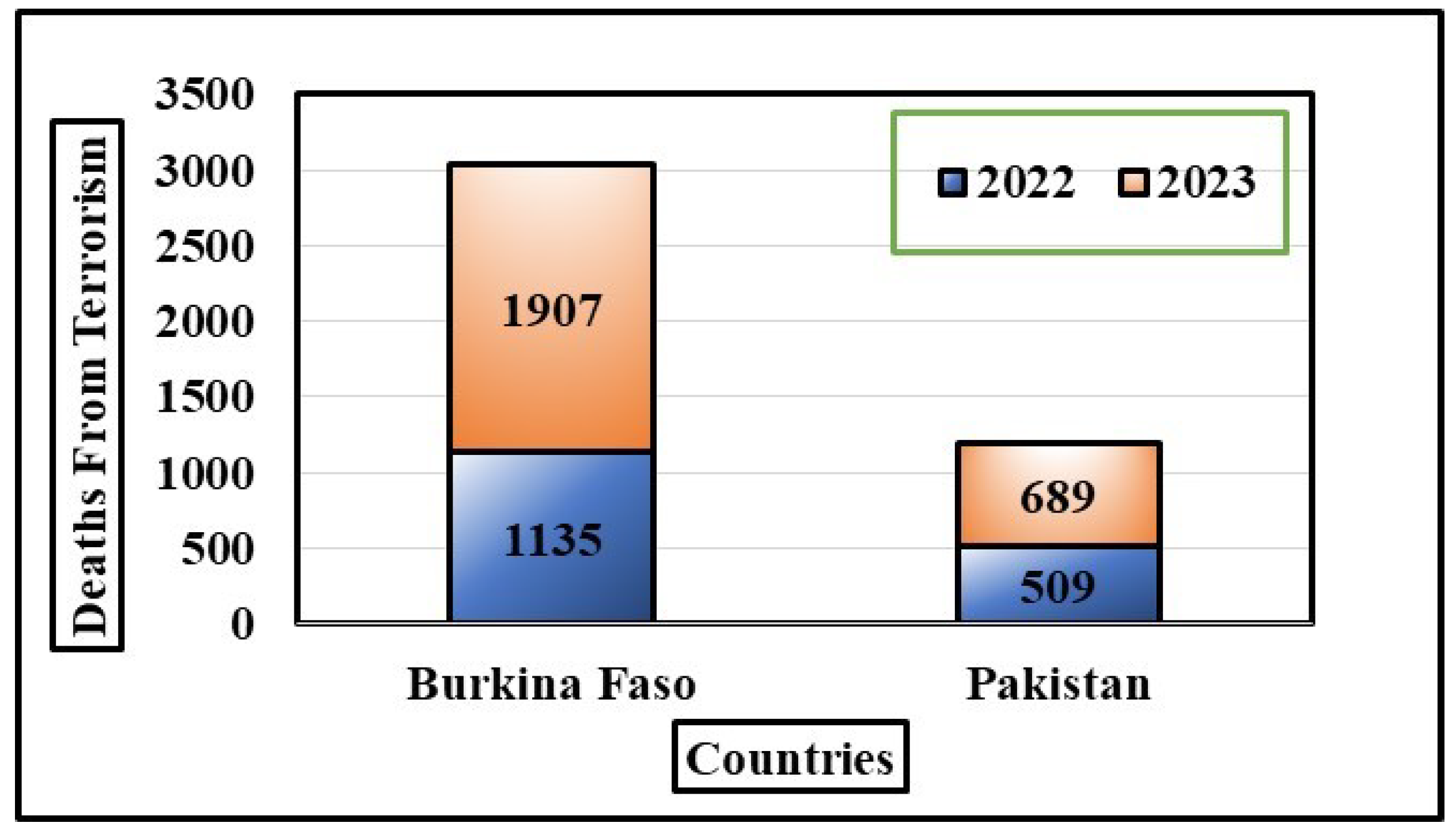
Figure 1. Total terrorism deaths by country in 2022–2023.
Applsci 15 00690 g001
Figure 2. Bibliographic overview of research papers on concealed object detection.
Applsci 15 00690 g002
Figure 3. Trend in various architectures used for concealed weapon detection over last three years.
Applsci 15 00690 g003
Figure 4. PMMW imaging data samples. (a) Optical image with thick clothes. (b) PMMW image. (c) Optical image with thin clothes. (d) PMMW image containing concealed gun. (e) Real-time signature of metal gun.
Applsci 15 00690 g004
Figure 6. Flowchart of proposed alpha-reshuffled bootstrap random sampling method.
Applsci 15 00690 g006
Figure 7. Comparison between the original and filtered images. (ad) Original images. (eh) Filtered images.
Applsci 15 00690 g007
Figure 8. YOLOv8 algorithm.
Applsci 15 00690 g008
Figure 9. The architecture of proposed YOLOv8 algorithm.
Applsci 15 00690 g009
Figure 10. The architectures of the FER and Conv_Reg modules. (a) FER module. (b) Conv_Reg module.
Applsci 15 00690 g010
Figure 11. Proposed framework of research methodology.
Applsci 15 00690 g011
Figure 12. The proposed FER-YOLOv8 architecture’s configuration.
Applsci 15 00690 g012
Figure 13. Confusion matrices of various YOLO models. (a) Tiny YOLOv3. (b) YOLOv8n. (c) YOLOv8m. (d) YOLOv8n-WF. (e) YOLOv8m-WF. (f) Proposed FER-YOLOv8.
Applsci 15 00690 g013
Figure 14. Comparison of mean average precision of various models in percent (%).
Applsci 15 00690 g014
Figure 15. Comparison of mean average precision (mAP) of IoU thresholds ranging from 0.5 to 0.95 of various models in percent (%).
Applsci 15 00690 g015
Figure 16. Comparison of F1-confidence curves of various YOLO models. (a) Tiny YOLOv3 F1-confidence curves. (b) YOLOv8n F1-confidence curves. (c) YOLOv8n-WF F1-confidence curves. (d) YOLOv8m F1-confidence curves. (e) YOLOv8m-WF F1-confidence curves. (f) Proposed FER-YOLOv8 F1-confidence curves.
Applsci 15 00690 g016
Figure 17. Precision–recall curves of tiny YOLOv3 and proposed FER-YOLOv8 models. (a) Tiny YOLOv3 PR curves. (b) Proposed FER-YOLOv8 PR curves.
Applsci 15 00690 g017
Figure 18. Comparison of precision–recall curves of various YOLO models. (a) YOLOv8n PR curves. (b) YOLOv8n-WF PR curves. (c) YOLOv8m PR curves. (d) YOLOv8m-WF PR curves.
Applsci 15 00690 g018
Figure 19. Comparison of computational complexity of various YOLO models.
Applsci 15 00690 g019
Figure 20. Qualitative analysis of the trained models on an accurately detected positive sample. (a) Positive sample from ground truth. (b) Tiny YOLOv3 prediction. (c) YOLOv8n prediction. (d) YOLOv8n-WF prediction. (e) YOLOv8m prediction. (f) YOLOv8m-WF prediction. (g) Proposed FER-YOLOv8 prediction.
Applsci 15 00690 g020
Figure 21. Violin plots showing the distribution of the confidence scores of various models on a test dataset. (a) Tiny YOLOv3 confidence score distribution. (b) YOLOv8n confidence score distribution. (c) YOLOv8n-WF confidence score distribution. (d) YOLOv8m confidence score distribution. (e) YOLOv8m-WF confidence score distribution. (f) Proposed FER-YOLOv8 confidence score distribution.
Applsci 15 00690 g021
Figure 22. Qualitative analysis of the trained models on the falsely detected positive sample. (a) Negative sample from ground truth. (b) Tiny YOLOv3 prediction. (c) YOLOv8n prediction. (d) YOLOv8n-WF prediction. (e) YOLOv8m prediction. (f) YOLOv8m-WF prediction. (g) Proposed FER-YOLOv8 prediction.
Applsci 15 00690 g022
Figure 23. Comparison of feature maps of first layer of various YOLO models.
Applsci 15 00690 g023
Table 1. Hyperparameter settings of various YOLO architectures.
ModelsHyperparameter
Tiny YOLOv3, YOLOv8n, and YOLOv8mEpoch: 100
Batch size: 16
Learning rate: 0.01
Final learning rate: 0.01
Momentum: 0.9
weight_decay = 0.0005
Optimizer: AdamW
Patience: 100
Proposed FER-YOLOv8Dropout rate: 20%
Epoch: 100
Batch size: 16
Learning rate: 0.01
Final learning rate: 0.01
Momentum: 0.9
weight_decay = 0.0005
Optimizer: AdamW
Patience: 100
Table 2. Initial structure of a backbone network in the proposed FER-YOLOv8 architecture.
ModuleLayerInput ChannelsOutput ChannelsParametersSize/StrideOutput
FERConvolutional38401 × 1/1640 × 640
Dropout--0-640 × 640
Conv_RegConvolutional84835523 × 3/2320 × 320
Dropout--0-320 × 320
Table 3. Comparison of precision metric for various classes.
ModelOverall Precision (%)Macro-Averaging Precision (%)Precision for Person Class (%)Precision for Gun Class (%)
Tiny YOLOv3 98.3 93.6 100.0 87.3
YOLOv8n 98.5 97.9 100.0 95.9
YOLOv8m 98.9 96.2 100.0 92.5
YOLOv8n-WF 98.0 96.9 100.0 93.9
YOLOv8m-WF 99.0 96.4 100.0 92.9
Proposed FER-YOLOv8 99.5 99.0 100.0 98.1
Table 4. Comparison of recall metric for various classes.
ModelOverall Recall (%)Macro-Averaging Recall (%)Recall for Person Class (%)Recall for Gun Class (%)
Tiny YOLOv3 98.4 97.6 100.0 95.2
YOLOv8n 98.8 98.2 100.0 96.5
YOLOv8m 98.9 98.4 100.0 97.2
YOLOv8n-WF 98.8 98.2 100.0 96.5
YOLOv8m-WF 98.7 98.1 100.0 97.2
Proposed FER-YOLOv8 99.3 99.0 100.0 98.1
Disclaimer/Publisher’s Note: The statements, opinions and data contained in all publications are solely those of the individual author(s) and contributor(s) and not of MDPI and/or the editor(s). MDPI and/or the editor(s) disclaim responsibility for any injury to people or property resulting from any ideas, methods, instructions or products referred to in the content.