Abstract
Pedestrian trajectories are crucial for self-driving cars to plan their paths effectively. The sensors implanted in these self-driving vehicles, despite being state-of-the-art ones, often face inaccuracies in the perception of surrounding environments due to technical challenges in adverse weather conditions, interference from other vehicles’ sensors and electronic devices, and signal reception failure, leading to incompleteness in the trajectory data. But for real-time decision making for autonomous driving, trajectory imputation is no less crucial. Previous attempts to address this issue, such as statistical inference and machine learning approaches, have shown promise. Yet, the landscape of deep learning is rapidly evolving, with new and more robust models emerging. In this research, we have proposed an encoder–decoder architecture, the Human Trajectory Imputation Model, coined HTIM, to tackle these challenges. This architecture aims to fill in the missing parts of pedestrian trajectories. The model is evaluated using the Intersection drone the inD dataset, containing trajectory data at suitable altitudes, preserving naturalistic pedestrian behavior with varied dataset sizes. To assess the effectiveness of our model, we utilize L1, MSE, and quantile and ADE loss. Our experiments demonstrate that HTIM outperforms the majority of the state-of-the-art methods in this field, thus indicating its superior performance in imputing pedestrian trajectories.
1. Introduction
Pedestrian trajectory unpredictability has presented a formidable challenge for autonomous vehicles, necessitating sophisticated trajectory imputation techniques. The erratic and dynamic nature of pedestrians’ movement makes it challenging to accurately predict their future paths. Factors such as sudden changes in direction, varying speeds, and unexpected interactions with the environment contribute to this unpredictability. Figure 1 Bearing this unpredictability in mind, autonomous vehicles have transformed transportation by utilizing state-of-the-art technologies like artificial intelligence, sensor fusion, and machine learning to navigate safely and independently. Central to their operation is the ability to efficiently plan and follow trajectories while adapting to changing environments. In this context, a trajectory refers to the path an entity takes over time, including its spatial coordinates, velocity, and orientation. Mathematically, a trajectory describes the vehicle’s state in a specific coordinate system, where denotes its position, represents its velocity, and indicates its heading at time t. Trajectory imputation is a critical aspect of motion prediction, focusing on filling in missing points within incomplete trajectories to create a comprehensive representation of an object’s movement. Essentially, trajectory imputation involves using existing trajectory data to interpolate or extrapolate missing segments, compensating for factors like sensor errors, occlusions, or data loss. By integrating predictive models with historical trajectory information, trajectory imputation facilitates the reconstruction of a coherent and uninterrupted trajectory, vital for applications such as autonomous navigation and activity recognition. The primary objective of trajectory imputation is to estimate the missing points inside the incomplete trajectory to yield a complete trajectory represented as follows:
and
where 1 represents the number of missing points to be imputed, n denotes the total points of a complete trajectory, and m is a variable providing the continuity of sequential points.
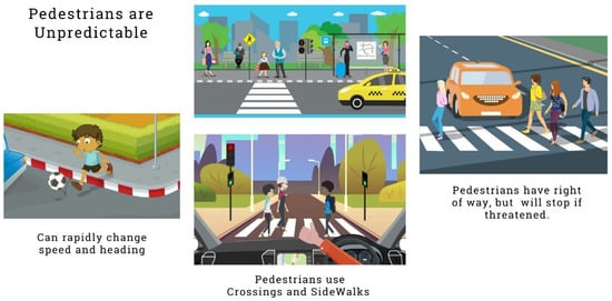
Figure 1.
Humans are unpredictable, a critical security concern for autonomous vehicles. Image courtesy of coursera.org accessed on 25 June 2024.
Since the early days of trajectory imputation, several techniques have been employed, each with its advantages and limitations. These techniques include Kalman filtering [1], which is widely used for state estimation and trajectory prediction in autonomous vehicles. It provides a recursive solution for predicting the phase of a dynamic system dependent on noisy sensor measurements. Kalman filters are particularly effective in scenarios with linear dynamics and Gaussian noise distributions. Particle filters, also known as Monte Carlo localization [2], are probabilistic algorithms used for non-linear and non-Gaussian state estimation. They represent the posterior distribution of the vehicle’s state using a set of weighted particles. These particles are sampled and propagated based on motion models and sensor measurements. Bayesian inference provides a principled framework for updating beliefs about the vehicle’s state based on observed data and prior knowledge. It allows for the incorporation of uncertainty into trajectory prediction and facilitates decision making under uncertainty.
In recent times, machine learning methodologies, like support vector machines [3], neural networks, and Gaussian processes, have been increasingly employed for trajectory imputation in autonomous vehicles. These approaches learn complex relationships from data and can capture intricate patterns in vehicle motion and environmental interactions. The advancement of deep learning [4] fields has significantly influenced trajectory imputation in autonomous vehicle systems. Deep learning techniques have demonstrated remarkable capabilities in capturing intricate patterns and dependencies within trajectory data, leading to enhanced prediction accuracy and robustness. Several key techniques have emerged that harness the strength of deep learning models. Recurrent neural networks (RNNs), particularly Gated Recurrent Units (GRUs) and long–short-term memory (LSTM), and several of LSTM’s variants, like bidirectional LSTM (Bi-LSTM) [5], attention-based LSTM (AttLSTM) [6], stacked LSTM [7], convolutional LSTM (ConvLSTM) [8], LSTM with temporal convolutional networks (TCNs) [9], and peephole LSTM [10], have gained prominence in trajectory imputation tasks.
As we stated earlier, despite advancements in trajectory prediction, accurately imputing pedestrian trajectories remains a significant challenge due to the inherent unpredictability of human movement. Traditional techniques like Kalman filters and particle filters have limitations in handling non-linear and non-Gaussian dynamics, while existing machine learning models often struggle with complex, crowded environments and missing data. There is a critical need for a robust trajectory imputation method that can effectively handle the erratic nature of pedestrian movement and provide accurate predictions in real time.
Our research has made the following noteworthy contributions to this field of research:
- We have explored the challenges and requirements specific to trajectory interpolation for autonomous vehicles, considering the real-time nature and safety criticality of autonomous driving systems.
- We have utilized a masking process for converting complete trajectories into incomplete trajectories, which randomly eliminates a certain portion of points. This introduces more uncertainty and randomness, which ultimately enriches the training process.
- We have examined the use of LSTM and GRU in the travel path restoration of pedestrians, taking into consideration their propensity for managing temporal dependencies and contextual interactions.
- We have designed an encoder–decoder imputation model comprising LSTM blocks for the encoder and GRU blocks for the decoder.
- We have evaluated the effectiveness of our model on a curated version of inD dataset, marking one of the earliest instances of research on this dataset for the trajectory imputation task.
Section 2 provides an overview of the existing related literature. Section 3 identifies gaps in previous research. The dataset description and preprocessing methods are outlined in Section 4. Section 5 elaborates on the proposed methodology. The experimental results and a discussion are presented in Section 6. Finally, Section 7 presents the conclusions for the study and proposes avenues for future research. Moreover, Table 1 presents the symbols used in this paper.

Table 1.
Glossary of symbols and their definitions.
2. Related Work
Missing value handling is one of the most difficult problems in the field of time series data. A wide variety of approaches, from complex convolutional recurrent encoder–decoder architectures to recurrent dynamical systems, have been thoroughly explored by researchers. By studying the literature, we have examined different approaches used to fill the gaps in work related to time series datasets, exposing the advantages and disadvantages of each.
Using a bidirectional recurrent dynamical system, Cao et al. [11] described a technique for inferring time series data that can directly estimate the missing value. There was no significant presumption about the underlying data generation method. The majority of the other current systems, according to the paper, made significant assumptions about the data generation process. According to Kreindler et al. [12], there was no abrupt spike in the data and the data were smoothable while generating the missing data. Therefore, smoothing the surrounding data could produce missing values. Some current methods have used interpolation to infer missing values; however, local interpolation has generated missing values without taking into account the relationship between the variables over time. The model BRITS, devised in the literature, has outperformed all baseline models in terms of mean absolute error and mean relative error.
Nawaz et al. [13] introduced a deep learning-based convolutional recurrent encoder–decoder architecture to address the GPS trajectory imputation problems. There were temporal and spatial components to GPS trajectory data. While recurrent neural networks such as LSTM were effective in predicting consecutive time series, convolutional neural networks excelled at extracting the spatial aspect from data. They were used by the suggested ConvLSTM to achieve better results in trajectory imputation tasks. The authors used GPS trajectories with transportation mode labels from the Microsoft Geolife trajectory dataset [14,15,16] and employed the Average Displacement Error (ADE) as an evaluation metric.
Ma et al. [17] proposed a novel deep neural network approach to address the human trajectory imputation problem, which is a crucial step in the COVID-19 contact tracing process. The representation process using graph embedding was the first component of the solution, and the transformer model was the second. The formation of the human trajectory sequence occurred in a high-dimensional environment, making it difficult to extract significant information. The nodes were mapped from high-dimensional to low-dimensional vector space using the graph embedding model to remove the challenges. This aided in capturing the sequential aspect of human trajectory as well as the geo-spatial aspects. A deep CNN decoder, a softmax classifier, and a transformer encoder-based feature extractor made up the deep learning model. Because it can understand linkages and dependencies, the transformer’s main feature, Multi-head Self-Attention, confirmed that the sequence-to-sequence model exhibited good performance. The CRAWDAD unm/blebeacon [18] dataset, an open-source human mobility dataset, was used for the study.
The problem of trajectory prediction from partial observations owing to the misdetection of dynamic agents (cars, pedestrians, etc.), which can be brought on by poor image quality or occlusion by other dynamic agents, was studied by Fujii et al. [19]. The standard method for handling the incomplete trajectory problem has been to consider misdetection cases to be anomalies and remove them from the dataset. Because such a strategy eliminates the possibility of coordination with the agents that are excluded, there is a higher chance of major mishaps. Traditional methods for trajectory prediction have included those based on Bayesian filters. Their fundamental structure has made them unreliable for long-term prediction. RNNs, most notably, LSTM, are now widely used in modeling to anticipate human motions. The study by Fujii et al. proposed a two-block RNN for trajectory prediction from a partial trajectory due to misdetection, which learned the inference step of Bayesian filters. Two publicly accessible datasets, ETH [20] and UCY [21], were used in the experiment.
Almolegi et al. [22] introduced a novel model called Move, Attend, and Predict (MAP), which forecasts a person’s next location based on motions previously captured by a mobile device. The model used a deep neural network to identify the important components of mobility history for each location. The program also used an approach called embedding representation learning to extract relevant properties from the movement data. The model was tested on two big datasets and demonstrated that it outperformed other models in location prediction. The study solely took into account two types of input data: locations and timings. It ignored other elements that may impact people’s movements, such as preferences, social networks, weather, traffic, etc. The model was tested on two datasets: Geolife and Foursquare [23].
Wang et al. [24] introduced a novel deep learning approach to address the prevalent problem of missing trajectory data in GPS applications. Their proposed method leveraged an RNN with an encoder–decoder architecture and an attention mechanism [25]. To enhance data reconstruction quality, they introduced a new loss function based on the R2 coefficient and implemented a smoothing technique using a moving average and a Savitzky–Golay filter [26]. Evaluating their model on a real-world GPS dataset from the Geolife project, comprising 17,621 trajectories collected over five years from 182 users, they demonstrated its superiority over several baseline methods, including linear interpolation, cubic spline interpolation, a Kalman filter, LSTM, and Bi-LSTM in terms of recovery accuracy and result stability across various missing rates and patterns. Additionally, through ablation tests and parameter sensitivity analysis, they validated the effectiveness of their model components and design choices, underscoring the potential of their deep learning approach for robust trajectory data reconstruction.
3. Gap Analysis
Table 2 provides a comprehensive analysis of the limitations found in previous research. The gap analysis of the reviewed literature underscores several notable limitations encountered in prior research. Notably, Nawaz et al. demonstrated effectiveness in identifying patterns in common scenarios, but their method may struggle with complex, crowded trajectory movements.
Table 2.
Gap analysis of the reviewed literature.
Additionally, Cao et al.’s [11] approach, despite enhancing predictive accuracy, introduces uncertainty and noise by treating missing values as variables. The transformer-based model by Ma et al. [17] exhibits promise with Bluetooth low-energy data but lacks exploration on other trajectory data types. Almolegi et al.’s [22] MAP model faces constraints in handling new or unseen locations, while Fujii et al.’s [19] Bayesian filter framework adds complexity, potentially impacting scalability. Moreover, Wang et al.’s [24] model, leveraging an RNN with an encoder–decoder architecture, may overlook comprehensive performance assessment due to limited evaluation metrics. These findings underscore the necessity for further research to address these limitations comprehensively.
4. Dataset Observation and Prepossessing
In this section, we explore the dataset collection, observation, and prepossessing carried out as part of this research, providing a detailed overview of the steps taken to collect and prepare these data.
4.1. Dataset Observation
Various trajectory datasets exist for road users, but very few have met the needs of autonomous driving research. Examples include BIWI Walking Pedestrians [20], Stanford Drone [27], CITR and DUT [28], highD [29], Interaction [30], and Ko-PER [31]. Most lack sufficient data or public road scenarios. The inD dataset [32] is a new and unique dataset of naturalistic vehicle trajectories recorded at German intersections using a drone. The dataset includes more than 11,500 road users, including vehicles, bicyclists, and pedestrians, at four different locations (Braunschweig, Frankfurt, Lindau, Wurzburg) with varying traffic density and complexity. Table 3 shows a comparison of the inD dataset with other datasets [32].
Table 3.
Overview of trajectory data and characteristics.
The inD dataset surpasses other datasets in capturing naturalistic road user behavior due to its strategic design principles:
- Preserving naturalistic behavior: By avoiding visible sensors resembling traffic surveillance cameras, the inD dataset ensures road users are not impacted by the measurement method.
- Having satisfactory size: The inclusion of trajectories from thousands of road users provides the necessary size and variety for robust data-driven algorithms.
- Differentiating recording locations and times: The inD dataset captures measurements from multiple sites and diverse times of day, including public roads, ensuring the coverage of different road layouts, densities, and traffic rules for enhanced significance in automated driving scenarios.
- Detecting and tracking all road user types: Unlike datasets that limit themselves to specific categories, the inD dataset tracks all road users and recognizes the vital importance of capturing interactions across diverse user types.
- Tracking road users with top accuracy: The inD dataset guarantees trajectories with a positioning inaccuracy of less than 0.1 m, regardless of road user type, ensuring precision in capturing the intricacies of user movement.
- Including infrastructure details: With the precise recording of road layouts and local traffic rules, the inD dataset acknowledges the dependency of road user behavior on these factors, providing comprehensive information within the dataset.
4.2. Using Curated Dataset Prepared for Autonomous Vehicles
Muktadir et al. [33,34] dealt with human trajectories while keeping the concerns of autonomous vehicles in mind. Pedestrians walking by the side of each road should not be our concern. Road crossing pedestrians’ trajectories should be our focal point, as only then does the factor of autonomous vehicles come into play. Only by incorporating the trajectories of road-crossing pedestrians could they create a curated dataset, which we have used [33].
4.3. Making Incomplete Trajectories
In this section, we present our approach to creating incomplete trajectories through a masking strategy. We aim to simulate missing data in the trajectory sequences, which will be used during training.
4.3.1. Masking Strategy
To simulate missing data in trajectory sequences, we employ a comprehensive masking strategy that involves randomly selecting and discarding segments of the trajectory. This method ensures that the simulated missing data reflect realistic scenarios of incomplete data in trajectory analysis. Let represent a complete trajectory with T data points, where denotes the data point at time step t. We define the masking strategy as follows:
- Masking Ratio (): We introduce a hyperparameter which represents the percentage of data points we want to mask in each trajectory. The value of is determined during training and can be fine-tuned for optimal performance.
- Random Selection: To simulate missing data, we randomly select a starting point within the trajectory and discard a segment with a length proportional to . This means that a contiguous portion of the trajectory is removed, simulating realistic missing data scenarios
4.3.2. Creating Incomplete Trajectories
Using the described masking strategy, we generate incomplete trajectories from the complete ones. Let represent the resulting incomplete trajectory. We define the process mathematically as follows:
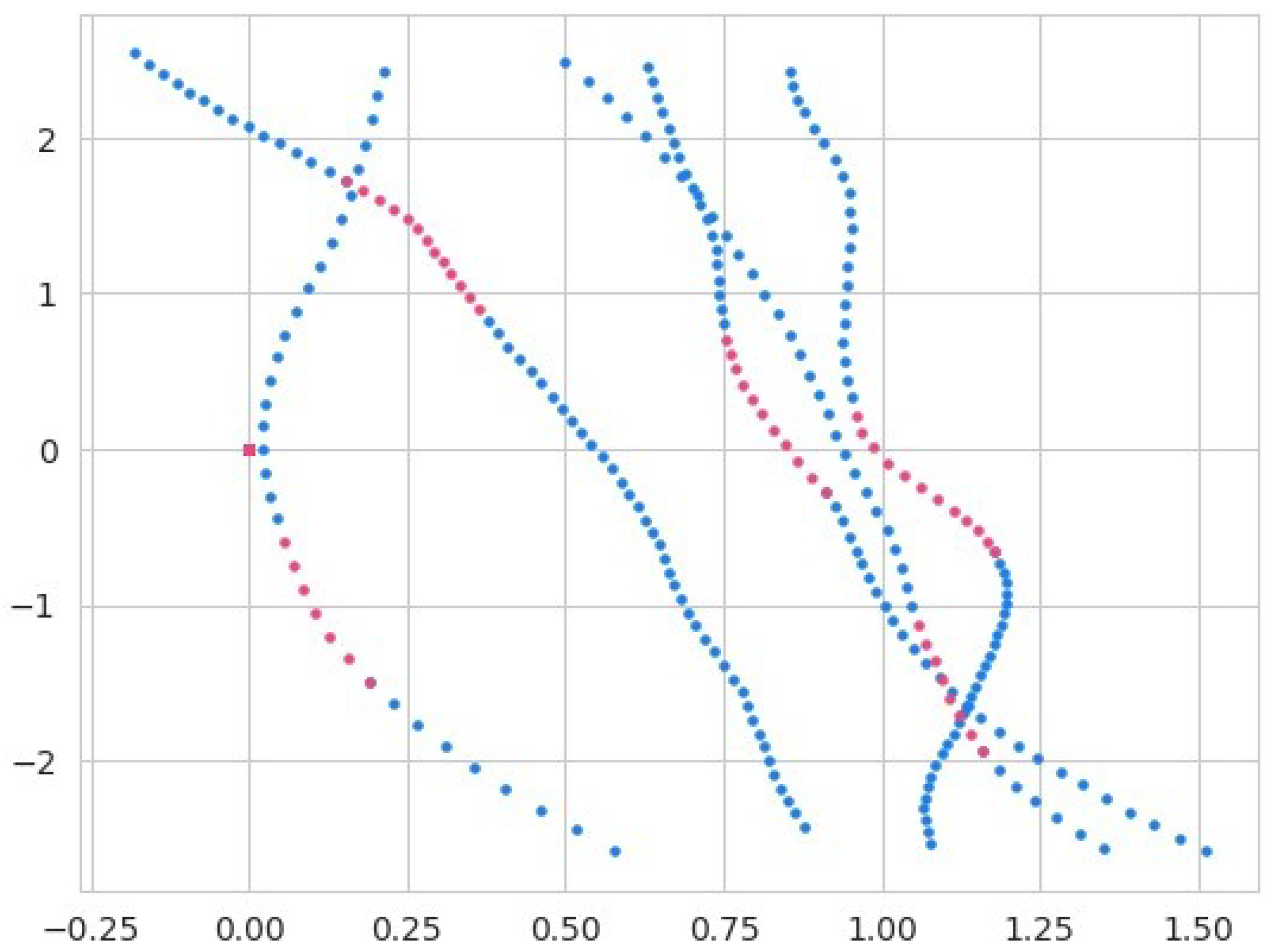
where is a function that applies the masking strategy to the complete trajectory with a masking ratio of . This function is designed to take a complete trajectory of any length, as trajectories can vary in length, and it will generate an incomplete trajectory by randomly discarding a certain portion of the trajectory. The hyperparameter is responsible for determining the proportion of the trajectory to be discarded. In Figure 2, the complete portions of the trajectories are presented in the color blue and the incomplete trajectories are represented by the red color.
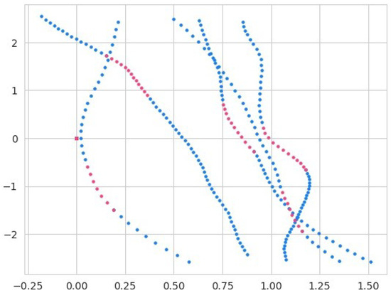
Figure 2.
The figure illustrates trajectory segmentation for the imputation process. The blue segments indicate the portions of the trajectory provided as input to the model, while the pink segments represent the randomly masked portions of the trajectory, which the model is tasked with imputing. This segmentation highlights the distinction between observed and unobserved data in the trajectory.
4.4. Padding and Binary Masking
The trajectories in the training dataset were padded to the maximum length across different trajectories from all four locations. This was a crucial step for efficient batch processing during training. Let represent the trajectory of the i-th example, and be its original length. The trajectories were padded to a length of , where .
Additionally, a binary mask was created for each trajectory to indicate the presence of observed points (1) and missing points (0) in the incomplete trajectories. The binary mask is denoted as , where if the point at time step t is observed and if it is missing.
5. Methodology
This section explores the complex structural characteristics of the methodology, providing thorough comprehension of the design elements and organizational components that are the basis of our approach.
5.1. LSTM Encoder–GRU Decoder Architecture with Teacher Forcing
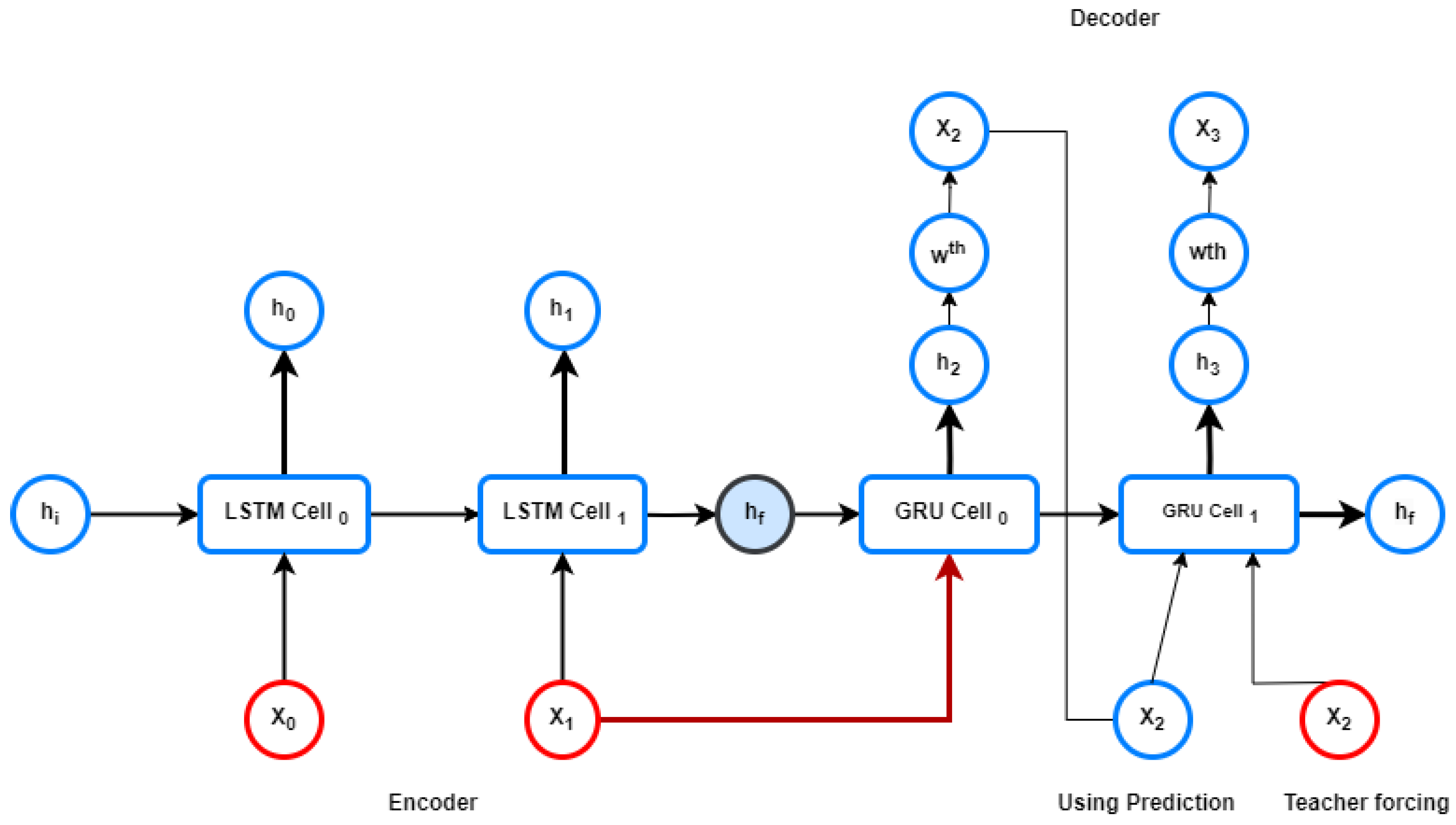
The LSTM-GRU (Gated Recurrent Unit)-based encoder–decoder (Figure 3) is a sequence-to-sequence model commonly used in various natural language processing and sequence generation tasks. As the name suggests, it consists of two main components, an encoder and a decoder. We picked LSTM for the the encoder part and GRU for the decoder after thorough experimentation.
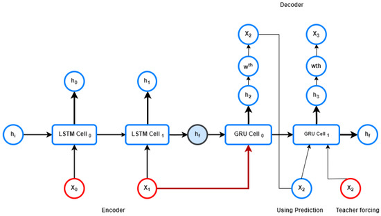
Figure 3.
Encoder-Decoder Architecture with Teacher Forcing: The red-labeled points represent the true outputs used during training.
5.1.1. LSTM Encoder
The LSTM encoder, a crucial component of sequence-to-sequence models, analyzes input sequences to capture their temporal dependencies. For an input sequence of length T, the encoder produces a hidden state sequence .
The LSTM encoder updates its hidden states using the following equations:
where denotes the logistic sigmoid function; ⊙ represents element-wise multiplication; stands for the input at time step t; represents the hidden state at time step t; , , , and denote the input, forget, cell, and output gates at time step t, respectively; and W and b represent the weight and bias matrices for different gates. represents the cell state at time step t. The LSTM’s unusual architecture, comprising input, forget, cell, and output gates, allow it to successfully capture long-range relationships in sequential data, making it well suited for jobs requiring memory retention over longer periods. The LSTM encoder is renowned for its ability to alleviate the vanishing gradient problem commonly encountered in traditional RNNs. This is achieved through its sophisticated gating mechanisms, which regulate the flow of information across time steps. The input gate controls the influx of fresh information into the cell state , while the forget gate regulates the confinement of former cell state information. The output gate governs the flow of information from the cell state to the hidden state, ensuring that relevant information is propagated forward while irrelevant information is suppressed.
5.1.2. GRU Decoder with Teacher Forcing
The GRU decoder with teacher forcing is responsible for generating an output sequence based on the hidden states obtained from the encoder. Given the hidden state sequence and an input sequence of length U, the decoder computes an output sequence .
The GRU decoder updates its hidden states and produces the output using the following equations, incorporating the concept of teacher forcing:
where GRU represents the operation of a Gated Recurrent Unit; denotes the logistic sigmoid function; ⊙ represents element-wise multiplication, is the input at time step t; represents the hidden state at time step t; and denote the reset and update gates, respectively; is the candidate hidden state; W and U are weight matrices; and b is a bias vector. Regressor is a function that maps the hidden state to the output space.
The GRU decoder with teacher forcing employs the use of teacher forcing, a technique where the decoder receives the true values of the previous time steps as inputs during training instead of its predictions. This technique facilitates learning by providing more accurate guidance to the model during training. The probability of using teacher forcing at each time step can be controlled by a parameter , where indicates full teacher forcing (always using true values), and indicates no teacher forcing (always using model predictions). The probability of using teacher forcing at time step t can be expressed as follows:
Thus, the input to the decoder is determined by whether teacher forcing is applied or not:
where represents the predicted output of the decoder at time step .
5.1.3. Justification for Using GRU
- Sequential Modeling: Because each point in a trajectory depends on the ones before it, trajectory data are inherently sequential. GRUs excel at sequential modeling as they maintain a hidden state that evolves, allowing them to capture dependencies in sequential data.
- Memory Cells with Gates: GRUs are equipped with memory cells and gating mechanisms, enabling them to reset and update their internal state dynamically. The reset gate allows the model to choose which historical data to disregard, while the update gate determines which fresh data to incorporate. This flexibility mitigates the vanishing gradient issue and facilitates the capture of long-term interdependencies.
- Efficient Training: GRUs are designed for computational efficiency, making them suitable for handling lengthy sequences often encountered in trajectory data. The efficiency of GRUs may contribute to quicker convergence during training.
- Parameter Efficiency: Compared to LSTM networks, GRUs have fewer parameters, enhancing their parameter efficiency. This characteristic is particularly beneficial when working with trajectory data that may have limited samples. The reduced number of parameters helps prevent overfitting and may lead to better generalization for new trajectories.
5.2. Training
Training the trajectory imputation model involves several key components that contribute to its overall performance. In this subsection, we elaborate on some crucial parts of the training phase, like the optimization strategy, gradient clipping, and learning rate scheduler. But firstly, let us talk about the core training strategy. Incomplete trajectories are termed as features and corresponding missing points are termed as labels. This is how the training was performed, so during the testing phase, given some incomplete trajectories, we obtained the missing points of corresponding trajectories as outputs. The dataset was split into training, validation, and testing sets using a ratio of 70% for training, 15% for validation, and 15% for testing
- OptimizationTo update the model parameters, an Adam optimizer was utilized. The Adam optimization algorithm computed the adaptive learning rates for each parameter based on their first-order moment estimate (mean) and the second-order moment estimate (uncentered variance). The update rule for the parameters is given bywhere and are the biased first- and second-moment estimates, is a small constant to prevent division by zero, and lr is the learning rate.
- Gradient ClippingGradient clipping was employed to prevent exploding gradients during backpropagation. This technique involves scaling the gradients if their norm exceeds a predefined threshold (max_grad_norm). The scaled gradient was computed as follows:
- Learning Rate SchedulerThe learning rate was scheduled using the ReduceLROnPlateau (a PyTorch library function which decreases learning rate when a metric has ceased improving) scheduler. This scheduler adjusted the learning rate if the validation losses plateaued, enabling the model to fine-tune its parameters more effectively. The learning rate update rule is given by:where is the previous learning rate, and factor is a user-defined factor.
5.3. Hyperparameters
In this subsection, we define and elaborate on the hyperparameters used in the trajectory imputation model. Hyperparameters are essential for influencing how the model behaves and performs during training. The hyperparameters are divided into two categories: model parameters, which define the model’s architecture, and training parameters, which affect how the model learns.
5.3.1. Model Parameters
- Dimensionality of input trajectories: This parameter represents the number of features or dimensions in the input data.
- Number of hidden units: The hidden size determines the ability of the model to grasp and represent temporal dependencies.
- Dimensionality of output trajectories: Similar to input size, this parameter defines the number of features in the output predictions.
- Number of layers: This parameter controls the depth of the recurrent neural network, influencing its ability to model complex patterns.
5.3.2. Training Parameters
- Gradient clipping threshold: For gradients during backpropagation, this value establishes the highest permitted norm. It improves training stability and helps stop gradients from blowing up.
- Maximum gradient norm for scaling gradients: Gradient clipping is applied to limit the norm of gradients. If the computed norm exceeds the limit, the gradients are scaled to meet this threshold.
Together, these hyperparameters form the trajectory imputation model’s design and training behavior. To achieve best performance and robustness during training, these variables must be fine-tuned.
6. Experimental Results and Discussion
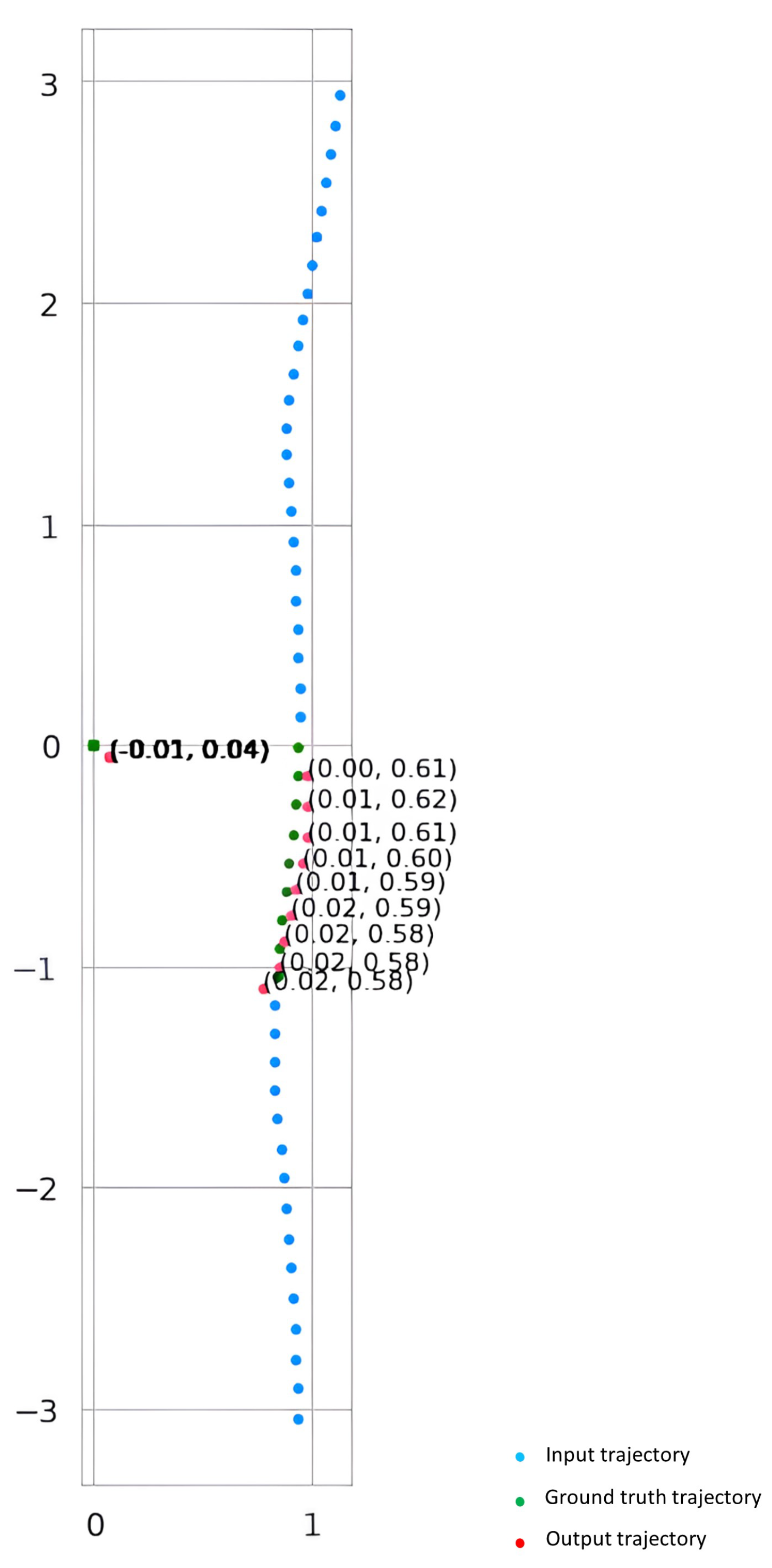
The “Results and Discussion” section outlines the model’s performance, highlighting significant metrics such as L1 loss and ADE. Graphical representations, including trend plots and a table of training results, provide a thorough picture. Table 4 showcases the minimum values for different metrics. Figure 4 clearly illustrates the model’s ability to predict and finish trajectories.
Table 4.
Summary of experimental results (minimum values).

Figure 4.
Comparison of generated and ground truth trajectories with velocity values.
6.1. L1 Loss
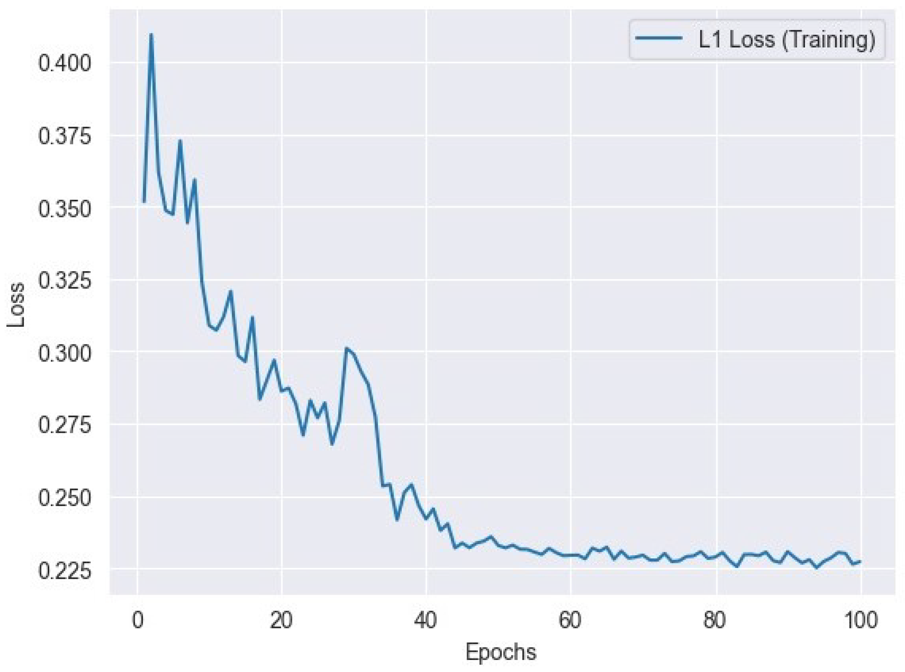
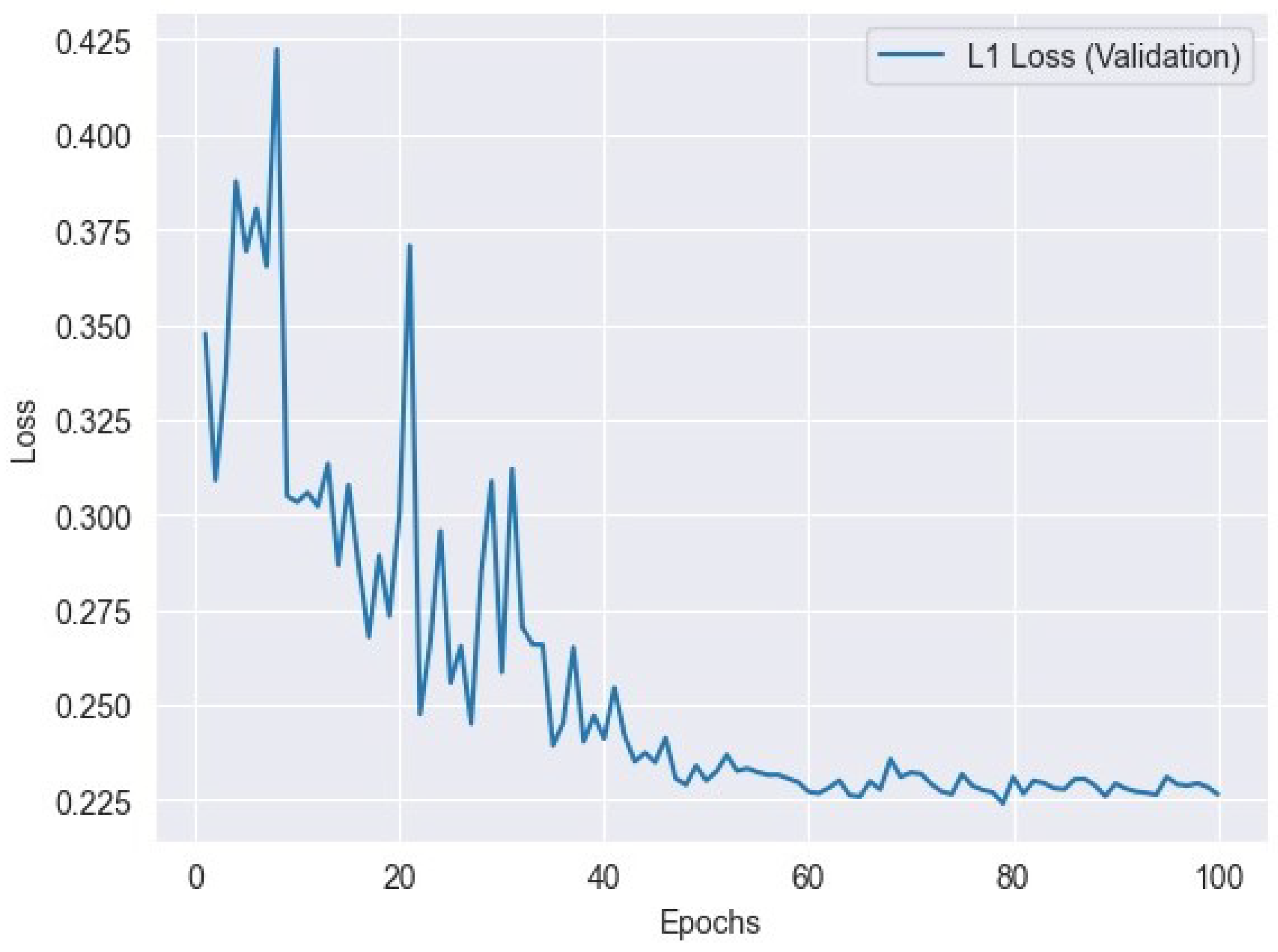
L1 loss, sometimes referred to as the mean absolute error (MAE) or L1 norm loss, is a commonly employed loss function in the fields of machine learning and optimization, specifically in regression problems. This metric measures the absolute disparities between the anticipated values and the actual target values for a total of n data points. L1 loss is calculated by taking the absolute difference between the predicted value () and the actual value () for each data point, and then averaging these differences across the total number of data points (n). The inclusion of the absolute value in this formula ensures that both overestimates and underestimates have an equal impact on the loss. L1 loss exhibits lower sensitivity to outliers in comparison to L2 loss (mean squared error), rendering it appropriate for situations where the influence of outliers on the total loss should be constrained. Figure 5 represents L1 training loss and Figure 6 represents L1 validation loss.
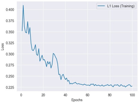
Figure 5.
L1 loss variation across training epochs: tracking the model’s performance.
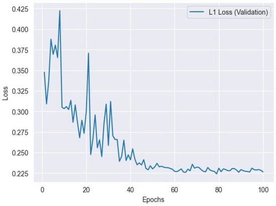
Figure 6.
L1 loss variation across validation epochs: tracking the model’s performance.
The L1 loss formula is given by
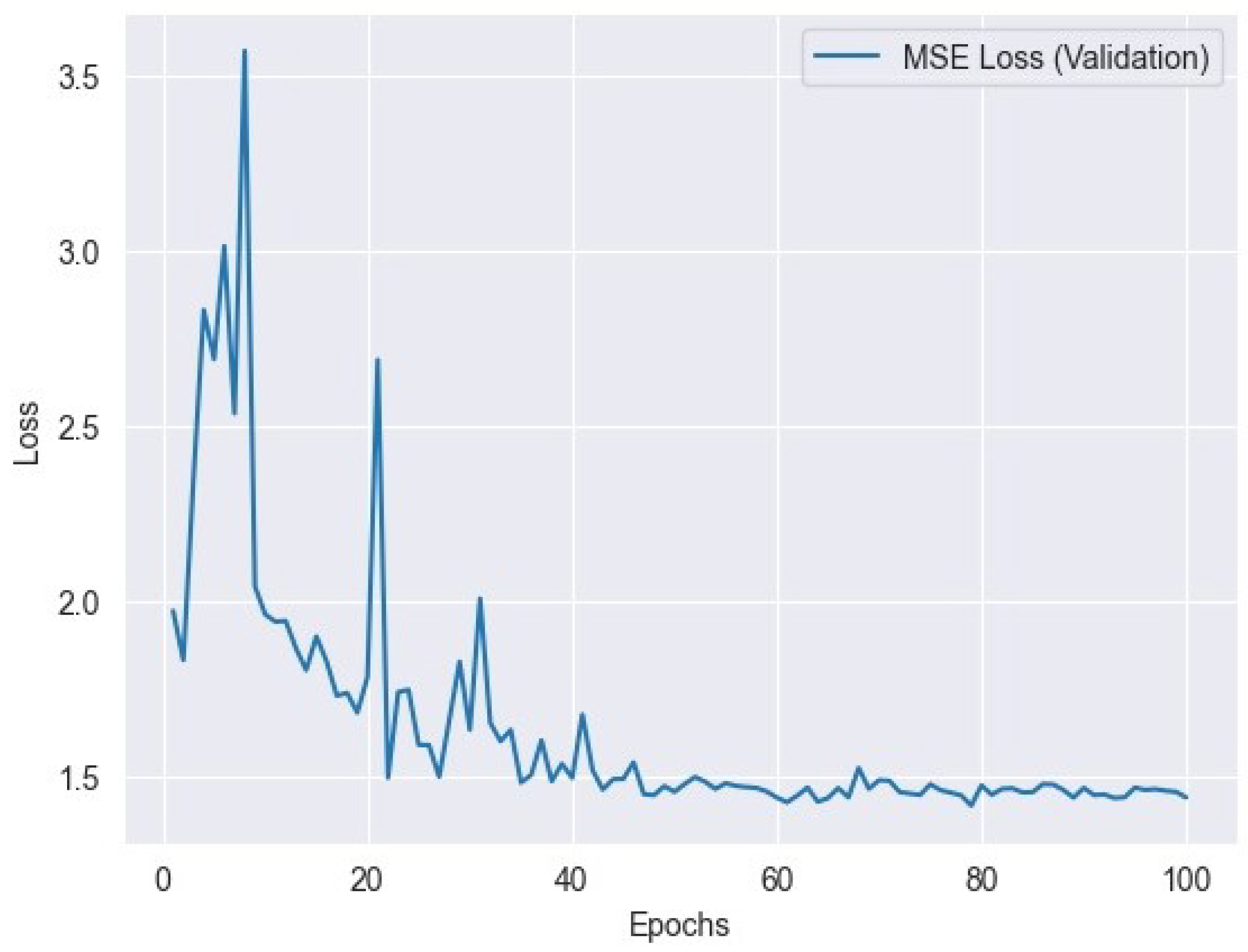
6.2. MSE Loss
Mean Squared Error (MSE) is a common metric used in regression analysis to measure the average squared difference between predicted values and actual values. MSE loss can be represented as follows:
where represents the actual value, represents the predicted value, and n is the number of data points. Figure 7 represents the MSE training loss and Figure 8 represents the MSE validation loss.
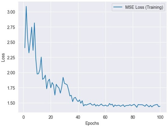
Figure 7.
MSE loss variation across training epochs: tracking the model’s performance.
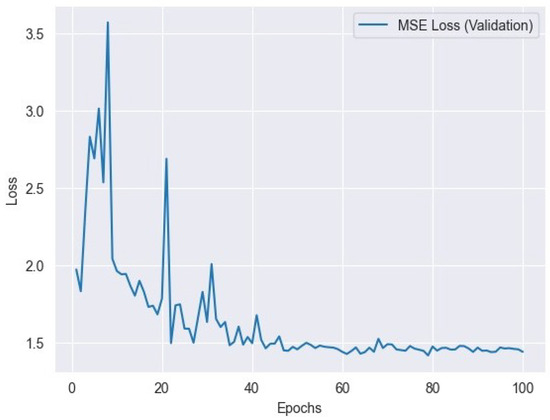
Figure 8.
MSE loss variation across validation epochs: tracking the model’s performance.
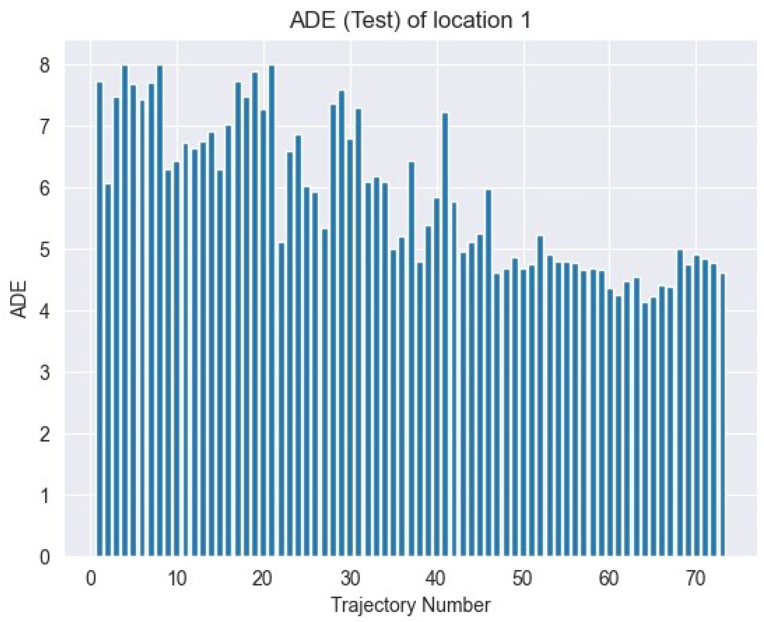
6.3. ADE Loss
Average Displacement Error (ADE) loss is a widely utilized statistic in trajectory prediction applications. This metric calculates the average Euclidean distance between anticipated points and their associated ground truth points throughout a series of frames. ADE loss is computed using the following formula:
where N is the total number of points in the sequence, represents the predicted position, and is the ground truth position. Figure 9 shows the ADE loss over time.
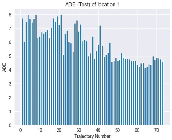
Figure 9.
ADE test loss: evaluation metric for model performance on test dataset.
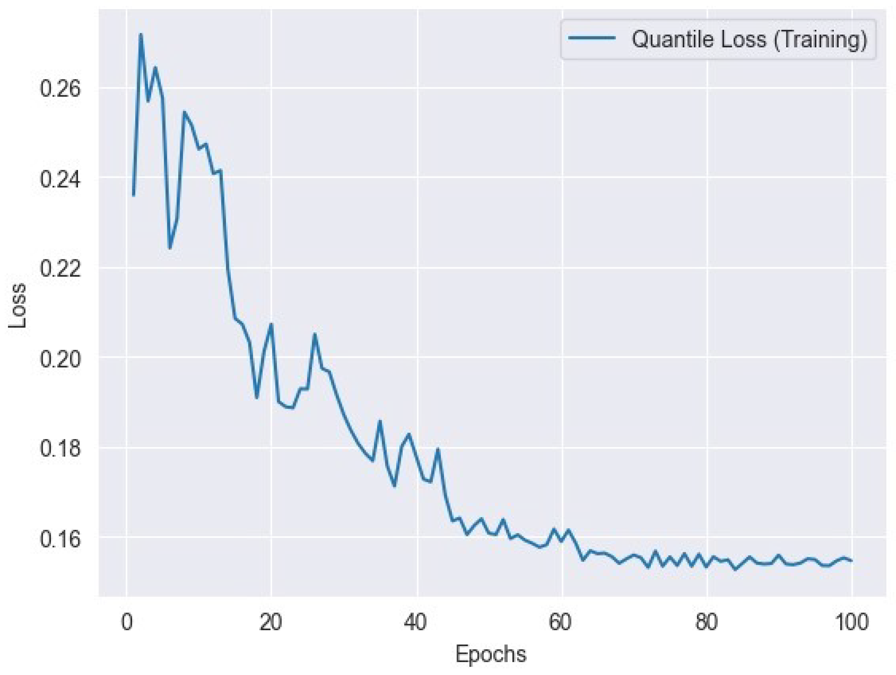
6.4. Quantile Loss
Quantile loss is a loss function used in quantile regression to measure the difference between predicted quantiles and actual quantiles of the target distribution. It is particularly useful when modeling non-normally distributed data or when different quantiles are of interest. Quantile loss is defined as
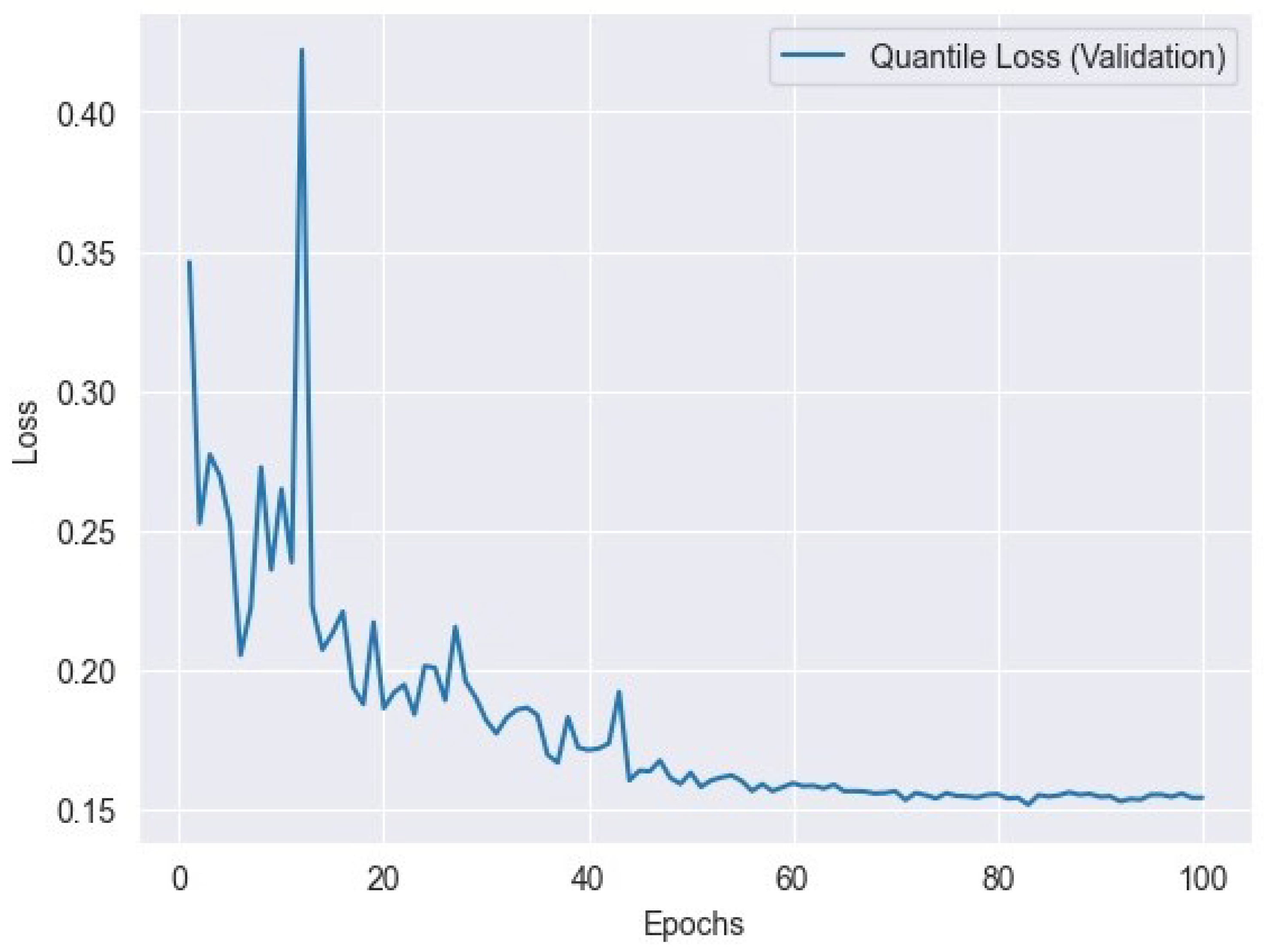
where represents the actual value, represents the predicted value, is the desired quantile level, and n is the number of data points. Figure 10 represents the quantile training loss, and Figure 11 represents the quantile validation loss.
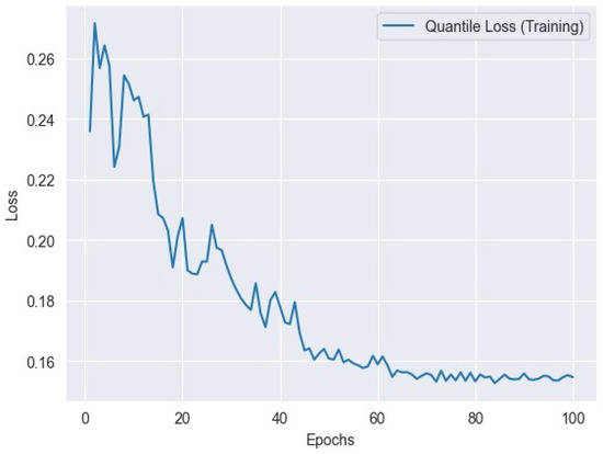
Figure 10.
Quantile loss variation across training epochs: tracking the model’s performance.
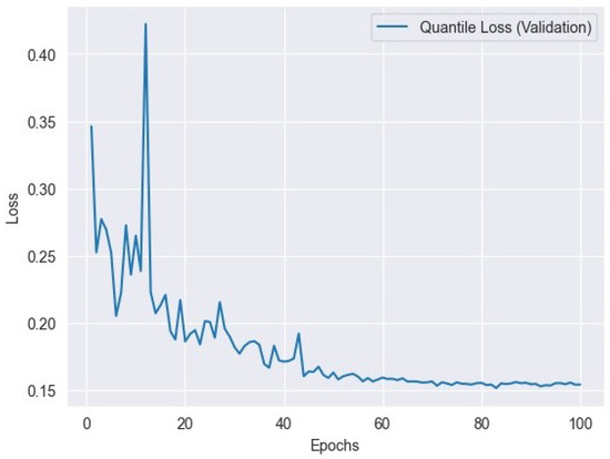
Figure 11.
Quantile loss variation across validation epochs: tracking the model’s performance.
Table 4 summarizes the minimum losses obtained from training, validation, and testing across various metrics. These minimum values provide insight into the performance achieved by the model at different evaluation stages.
6.5. Graphical Representations of Predicted Trajectory and Ground Truth Trajectory
In this subsection, we present a visual contrast between the predicted trajectory and the baseline trajectory. Figure 4 illustrates the trajectories plotted on a graph, with velocity values indicated. The x-axis represents the horizontal position, while the y-axis represents the vertical position. The blue line denotes the ground truth trajectory, while the red line represents the generated trajectory. Additionally, velocity values are annotated along the trajectories, providing insights into the speed variations throughout the movement. Arrows indicating the direction of movement are also included to enhance the visualization. This comparison allows for a qualitative assessment of the model’s performance in predicting trajectories and provides valuable insights into the dynamics of the system under study.
6.6. Comparison with Other Models
In this subsection, we conduct a comprehensive comparison of four models: a two-block RNN, BRITS, the GRU encoder–decoder, and our LSTM-GRU encoder–decoder model. The evaluation was primarily based on their respective L1 loss values, providing a quantitative measure of their performance.
In Table 5, the L1 loss values for each model are presented. The two-block RNN model yielded an L1 loss of 0.363, followed by BRITS with a loss of 0.312. The GRU-based encoder–decoder model exhibited an L1 loss of 0.306. Notably, our proposed LSTM-GRU encoder–decoder model outperformed the others with an impressively low L1 loss of 0.2264.
Table 5.
Models and their corresponding L1 loss.
7. Conclusions
In this research, we designed a novel deep learning model for imputing missing trajectory data for autonomous cars. Trajectory data are vital for the planning, navigation, and safety of autonomous cars, but they can be damaged or lost due to many circumstances, such as sensor failures, occlusions, noise, etc. Existing methods for trajectory imputation are either too straightforward, such as linear interpolation, or too complicated, such as generative adversarial networks.
We have proposed a hybrid model that incorporates LSTM and GRU to capture the temporal, spatial, and contextual characteristics of the trajectory data. Our model can handle different sorts of missing patterns and impute trajectories with excellent accuracy and efficiency. Long–short-term memory (LSTM) networks are renowned for their ability to retain long-term dependencies in sequential data. By employing an LSTM encoder, our model can effectively capture the temporal dynamics of trajectories. This means it can discern patterns and trends over extended periods, crucial for understanding how trajectories evolve over time.
On the decoding side, using a Gated Recurrent Unit (GRU) architecture brings its own advantages. GRUs are computationally efficient and can learn to adaptively update information in the decoding process. This helps in generating accurate predictions or reconstructions of trajectories while maintaining a balance between complexity and performance.
By fusing LSTM and GRU components, our model benefits from the strengths of both architectures. LSTM excels at retaining long-range dependencies, which is crucial for understanding complex trajectory patterns. On the other hand, GRU offers computational efficiency and simpler gating mechanisms, making it well suited for decoding tasks. This hybrid approach leverages the best of both worlds to enhance the overall performance and flexibility of the model.
The insights gained from trajectory analysis could be crucial for optimizing drone delivery routes in urban environments, where efficiency and safety are paramount. By leveraging trajectory analysis, logistics companies can minimize delivery times and maximize resource utilization, ultimately improving customer satisfaction and operational efficiency.
In future research endeavors, an intriguing avenue for enhancement involves experimenting with transformer models in the context of trajectory imputation for autonomous cars. Another limitation, which we have already mentioned in our study, is that it solely relies on the drone dataset, which is comparatively superior to other datasets in many arenas. But many studies have been carried out with the GPS and BLE datasets, which are no less important. Our model should be utilized on these datasets as a future path of exploration and experimentation. Also, we can experiment by adding different types of embeddings, like positional embedding or graph embedding with an attention mechanism, to our proposed architecture, and anticipate better outcomes in these cases.
Author Contributions
Conceptualization, D.K.B. and M.H.; methodology, D.K.B., M.H. and S.S.; software, S.S.; validation, D.K.B., M.H. and S.S.; formal analysis, D.K.B.; investigation, D.K.B.; resources, S.S; data curation, D.K.B., M.H and S.S; writing—original draft preparation, M.H. and D.K.B.; writing—review and editing, M.H. and D.K.B.; visualization, S.S.; supervision, M.M.I.; project administration, M.M.I.; funding acquisition, M.M.I. All authors have read and agreed to the published version of the manuscript.
Funding
This work was supported by the United International University (UIU) Institute of Advanced Research (IAR) Research Grant Scheme under Grant IAR-2024-Pub-016.
Institutional Review Board Statement
Not applicable.
Informed Consent Statement
Not applicable.
Data Availability Statement
Data is contained within the article.
Conflicts of Interest
The authors declare no conflicts of interest. The funders had no role in the design of the study; in the collection, analyses, or interpretation of data; in the writing of the manuscript; or in the decision to publish the results.
References
- Kalman, R.E. A New Approach to Linear Filtering and Prediction Problems. J. Basic Eng. 1960, 82, 35–45. [Google Scholar] [CrossRef]
- Dellaert, F.; Fox, D.; Burgard, W.; Thrun, S. Monte Carlo localization for mobile robots. In Proceedings of the 1999 IEEE International Conference on Robotics and Automation (Cat. No.99CH36288C), Detroit, MI, USA, 10–15 May 1999; Volume 2, pp. 1322–1328. [Google Scholar] [CrossRef]
- Cristianini, N.; Ricci, E. Support Vector Machines. In Encyclopedia of Algorithms; Kao, M.Y., Ed.; Springer: Boston, MA, USA, 2008; pp. 928–932. [Google Scholar] [CrossRef]
- Goodfellow, I.J.; Bengio, Y.; Courville, A. Deep Learning; MIT Press: Cambridge, MA, USA, 2016; Available online: http://www.deeplearningbook.org (accessed on 19 January 2024).
- Graves, A.; Fernández, S.; Schmidhuber, J. Bidirectional LSTM Networks for Improved Phoneme Classification and Recognition. In Proceedings of the Artificial Neural Networks: Formal Models and Their Applications–ICANN 2005, Warsaw, Poland, 11–15 September 2005; Duch, W., Kacprzyk, J., Oja, E., Zadrożny, S., Eds.; Springer: Berlin/Heidelberg, Germany, 2005; pp. 799–804. [Google Scholar]
- Liao, Y.; Lin, R.; Zhang, R.; Wu, G. Attention-based LSTM (AttLSTM) neural network for Seismic Response Modeling of Bridges. Comput. Struct. 2023, 275, 106915. [Google Scholar] [CrossRef]
- Ullah, M.; Ullah, H.; Khan, S.D.; Cheikh, F.A. Stacked Lstm Network for Human Activity Recognition Using Smartphone Data. In Proceedings of the 2019 8th European Workshop on Visual Information Processing (EUVIP), Rome, Italy, 28–31 October 2019; pp. 175–180. [Google Scholar] [CrossRef]
- Shi, X.; Chen, Z.; Wang, H.; Yeung, D.Y.; Wong, W.-k.; chun Woo, W. Convolutional LSTM Network: A Machine Learning Approach for Precipitation Nowcasting. arXiv 2015, arXiv:1506.04214. [Google Scholar] [CrossRef]
- Lea, C.; Vidal, R.; Reiter, A.; Hager, G.D. Temporal Convolutional Networks: A Unified Approach to Action Segmentation. In Proceedings of the Computer Vision–ECCV 2016 Workshops, Amsterdam, The Netherlands, 8–10 and 15–16 October 2016; Hua, G., Jégou, H., Eds.; Springer International Publishing: Cham, Switzerland, 2016; pp. 47–54. [Google Scholar]
- Deng, B.; Yan, J.; Lin, D. Peephole: Predicting Network Performance Before Training. arXiv 2017, arXiv:1712.03351. [Google Scholar] [CrossRef]
- Cao, W.; Wang, D.; Li, J.; Zhou, H.; Li, L.; Li, Y. BRITS: Bidirectional recurrent imputation for time series. In Advances in Neural Information Processing Systems 31; Curran Associates, Inc.: Red Hook, NY, USA, 2018. [Google Scholar]
- Kreindler, D.; Lumsden, C.J. The effects of the irregular sample and missing data in time series analysis. Nonlinear Dyn. Psychol. Life Sci. 2006, 102, 187–214. [Google Scholar]
- Nawaz, A.; Huang, Z.; Wang, S.; Akbar, A.; AlSalman, H.; Gumaei, A. GPS trajectory completion using end-to-end bidirectional convolutional recurrent encoder-decoder architecture with attention mechanism. Sensors 2020, 20, 5143. [Google Scholar] [CrossRef] [PubMed]
- Zheng, Y.; Liu, L.; Wang, L.; Xie, X. Learning Transportation Modes from Raw GPS Data for Geographic Application on the Web. In Proceedings of the International Conference on World Wide Web (WWW 2008), Beijing, China, 21–25 April 2008; pp. 247–256. [Google Scholar]
- Zheng, Y.; Li, Q.; Chen, Y.; Xie, X. Understanding Mobility Based on GPS Data. In Proceedings of the ACM Conference on Ubiquitous Computing (UbiComp 2008), Seoul, Republic of Korea, 21–24 September 2008; pp. 312–321. [Google Scholar]
- Zheng, Y.; Chen, Y.; Li, Q.; Xie, X.; Ma, W.-Y. Understanding Transportation Modes Based on GPS Data for Web Applications. Acm Trans. Web 2010, 4, 1–36. [Google Scholar] [CrossRef]
- Ma, J.; Yang, C.; Mao, S.; Zhang, J.; Periaswamy, S.C.; Patton, J. Human Trajectory Completion with Transformers. In Proceedings of the ICC 2022-IEEE International Conference on Communications, Seoul, Republic of Korea, 16–20 May 2022; IEEE: Piscataway, NJ, USA, 2022; pp. 3346–3351. [Google Scholar]
- Sikeridis, D.; Papapanagiotou, I.; Devetsikiotis, M. CRAWDAD Unm/Blebeacon. 2022. Available online: https://ieee-dataport.org/open-access/crawdad-unmblebeacon (accessed on 10 January 2024).
- Fujii, R.; Vongkulbhisal, J.; Hachiuma, R.; Saito, H. A two-block rnn-based trajectory prediction from incomplete trajectory. IEEE Access 2021, 9, 56140–56151. [Google Scholar] [CrossRef]
- Pellegrini, S.; Ess, A.; Schindler, K.; van Gool, L. You’ll never walk alone: Modeling social behavior for multi-target tracking. In Proceedings of the 2009 IEEE 12th International Conference on Computer Vision, Kyoto, Japan, 27 September–4 October 2009; IEEE: Piscataway, NJ, USA, 2009; pp. 261–268. [Google Scholar]
- Lerner, A.; Chrysanthou, Y.; Lischinski, D. Crowds by example. In ACM Transactions on Graphics (TOG); ACM: New York, NY, USA, 2007; Volume 26, pp. 1–10. [Google Scholar]
- Al-Molegi, A.; Jabreel, M.; Martínez-Ballesté, A. Move, Attend and Predict: An attention-based neural model for people’s movement prediction. Pattern Recognit. Lett. 2018, 112, 34–40. [Google Scholar] [CrossRef]
- Yang, D.; Zhang, D.; Yu, Z.; Yu, Z. Fine-grained preference-aware location search leveraging crowdsourced digital footprints from LBSNs. In Proceedings of the 2013 ACM International Joint Conference on Pervasive and Ubiquitous Computing, Zurich, Switzerland, 8–12 September 2013; ACM: New York, NY, USA, 2013; pp. 479–488. [Google Scholar]
- Wang, Z.; Zhang, S.; Yu, J.J. Reconstruction of Missing Trajectory Data: A Deep Learning Approach. In Proceedings of the 2020 IEEE 23rd International Conference on Intelligent Transportation Systems (ITSC), Virtual, 20–23 September 2020; pp. 1–6. [Google Scholar] [CrossRef]
- Soydaner, D. Attention mechanism in neural networks: Where it comes and where it goes. Neural Comput. Appl. 2022, 34, 13371–13385. [Google Scholar] [CrossRef]
- Yang, X.; Chen, J.; Guan, Q.; Gao, H.; Xia, W. Enhanced Spatial–Temporal Savitzky–Golay Method for Reconstructing High-Quality NDVI Time Series: Reduced Sensitivity to Quality Flags and Improved Computational Efficiency. IEEE Trans. Geosci. Remote Sens. 2022, 60, 1–17. [Google Scholar] [CrossRef]
- Robicquet, A.; Sadeghian, A.; Alahi, A.; Savarese, S. Learning Social Etiquette: Human Trajectory Understanding in Crowded Scenes. In Proceedings of the Computer Vision–ECCV 2016, Amsterdam, The Netherlands, 8–10 and 15–16 October 2016; Leibe, B., Matas, J., Sebe, N., Welling, M., Eds.; Springer International Publishing: Cham, Switzerland, 2016; pp. 549–565. [Google Scholar]
- Yang, D.; Li, L.; Redmill, K.; Ozguner, U. Top-view Trajectories: A Pedestrian Dataset of Vehicle-Crowd Interaction from Controlled Experiments and Crowded Campus. In Proceedings of the 2019 IEEE Intelligent Vehicles Symposium (IV), Paris, France, 9–12 June 2019; pp. 899–904. [Google Scholar] [CrossRef]
- Krajewski, R.; Bock, J.; Kloeker, L.; Eckstein, L. The highD Dataset: A Drone Dataset of Naturalistic Vehicle Trajectories on German Highways for Validation of Highly Automated Driving Systems. In Proceedings of the 2018 21st International Conference on Intelligent Transportation Systems (ITSC), Maui, HI, USA, 4–7 November 2018; pp. 2118–2125. [Google Scholar] [CrossRef]
- Zhan, W.; Sun, L.; Wang, D.; Shi, H.; Clausse, A.; Naumann, M.; Kümmerle, J.; Königshof, H.; Stiller, C.; de La Fortelle, A.; et al. INTERACTION Dataset: An INTERnational, Adversarial and Cooperative moTION Dataset in Interactive Driving Scenarios with Semantic Maps. arXiv 2019, arXiv:1910.03088. [Google Scholar] [CrossRef]
- Strigel, E.; Meissner, D.; Seeliger, F.; Wilking, B.; Dietmayer, K. The Ko-PER intersection laserscanner and video dataset. In Proceedings of the 2014 17th IEEE International Conference on Intelligent Transportation Systems, ITSC 2014, Qingdao, China, 8–11 October 2014; pp. 1900–1901. [Google Scholar] [CrossRef]
- Bock, J.; Krajewski, R.; Moers, T.; Runde, S.; Vater, L.; Eckstein, L. The inD Dataset: A Drone Dataset of Naturalistic Road User Trajectories at German Intersections. In Proceedings of the 2020 IEEE Intelligent Vehicles Symposium (IV), Las Vegas, NV, USA, 19 October–13 November 2020; pp. 1929–1934. [Google Scholar] [CrossRef]
- Muktadir, G.M.; Ikram, Z.; Whitehead, J. Pedestrian Crossing Dataset Extraction from InD Dataset. 2023; preprint. [Google Scholar] [CrossRef]
- Available online: https://github.com/adhocmaster/drone-dataset-tools (accessed on 7 March 2024).


Disclaimer/Publisher’s Note: The statements, opinions and data contained in all publications are solely those of the individual author(s) and contributor(s) and not of MDPI and/or the editor(s). MDPI and/or the editor(s) disclaim responsibility for any injury to people or property resulting from any ideas, methods, instructions or products referred to in the content. |
© 2025 by the authors. Licensee MDPI, Basel, Switzerland. This article is an open access article distributed under the terms and conditions of the Creative Commons Attribution (CC BY) license (https://creativecommons.org/licenses/by/4.0/).