Super Typhoons Simulation: A Comparison of WRF and Empirical Parameterized Models for High Wind Speeds

Abstract

As extreme forms of tropical cyclones (TCs), typhoons pose significant threats to both human society and the natural environment. To better understand and predict their behavior, scientists have relied on numerical simulations. Current typhoon modeling primarily falls into two categories: (1) complex simulations based on fluid dynamics and thermodynamics, and (2) empirical parameterized models. Most comparative studies on these models have focused on wind speed below 50 m/s, with fewer studies addressing high wind speed (above 50 m/s). In this study, we design and compare four different simulation approaches to model two super typhoons: Typhoon Surigae (2102) and Typhoon Nepartak (1601). These approaches include: (1) The Weather Research and Forecasting (WRF) model simulation driven by NCEP Final Operational Global Analysis data (FNL), (2) WRF simulation driven by the fifth generation of the European Centre for Medium-Range Weather Forecasts (ECMWF) reanalysis data (ERA5), (3) the empirical parameterized Holland model, and (4) the empirical parameterized Jelesnianski model. The simulated wind fields were compared with the measured wind data from The Soil Moisture Active Passive (SMAP) platform, and the resulting wind fields were then used as inputs for the Simulating WAves Nearshore (SWAN) model to simulate typhoon-induced waves. Our findings are as follows: (1) for high wind speeds, the performance of the empirical models surpasses that of the WRF simulations; (2) using more accurate driving wind data improves the WRF model’s performance in simulating typhoon wind speeds, and WRF simulations excel in representing wind fields in the outer regions of the typhoon; (3) careful adjustment of the maximum wind speed radius parameter is essential for improving the accuracy of the empirical models.

1. Introduction

Typhoons, as a severe form of tropical cyclones, pose significant threats to human society and the natural environment. The destructive power of typhoons is mainly manifested through three mechanisms: high winds, heavy rainfall, and storm surges. These direct impacts often lead to severe human casualties and substantial property losses. Situated within the primary impact zone of tropical cyclones in the Northwest Pacific, the areas surrounding Taiwan Island and the Philippines Peninsula experience significant loss of life and property each year due to typhoon events. According to the national standard for “Tropical Cyclone Categories” set by the China Meteorological Administration, typhoons are classified into six intensity levels: Tropical Depression (TD), Tropical Storm (TS), Severe Tropical Storm (STS), Typhoon (TY), Severe Typhoon (STY), and Super Typhoon (SuperTY). Among these, Super Typhoons are rare yet highly destructive natural disasters. Although their frequency of occurrence is relatively low, each event can cause significant damage to the affected areas. In particular, the impact of Super Typhoons is pronounced in the regions of Taiwan Island and the Philippine Peninsula, as well as their surrounding areas. Strong winds can lead to widespread crop damage and destruction of fishing facilities, while heavy rainfall may trigger flash floods that wash away roads and houses. These events severely disrupt the lives and economic development of residents. Given their immense potential for destruction and significant impact on human society, Super Typhoons must be given high priority and subjected to thorough research.

The study of typhoons has a long history, with its origins traceable to ancient times when people primarily relied on observing changes in wind direction to predict weather patterns. However, modern scientific research on typhoons began in the early 20th century. As the field of meteorology advanced, particularly with the widespread application of satellite remote sensing technology, humanity’s understanding of typhoons improved significantly [1,2,3]. The rapid development of computer technology in the 1970s further advanced numerical weather prediction models, leading to more precise forecasts of typhoon trajectories and intensities [4,5]. These developments have greatly improved the accuracy and reliability of typhoon forecasts, providing robust scientific support for disaster prevention and mitigation efforts.

Currently, scientists focus the numerical simulation research on typhoons within two primary domains. One approach emphasizes simulating complex physical processes based on fluid dynamics and thermodynamics, valued for its high accuracy. However, this method is computationally intensive. The Weather Research and Forecasting (WRF) model and the Fifth-Generation Penn State/NCAR Mesoscale Model (MM5) are commonly used tools for such research. Scientists have used the WRF and MM5 models for typhoon numerical simulations, validating their accuracy and conducting sensitivity analyses on various simulation parameter schemes [6,7,8,9,10]. Another method for typhoon simulation relies on theoretical and empirical formulas, or a combination of both, to calculate typhoon wind fields. Since the 1960s, numerous empirical parametric typhoon models have been developed by scholars, characterized by their relatively low computational demand [11,12,13,14]. Scientists have conducted a series of studies using these empirical parameterized typhoon models, including driving ocean models with the generated wind fields, comparing and blending them with reanalysis wind fields, and analyzing them alongside other wind field models [15,16,17].

The development of numerical simulation methods for super typhoons is ongoing. For instance, the Weather Research and Forecasting (WRF) model has been employed to numerically simulate the intensity and structure of super typhoons. The accuracy of these simulations is then validated using observational data [18,19]. Scientists have also been employing numerical simulation methods to investigate the factors contributing to the intensification of super typhoons. These factors include sea surface temperature (SST), sea–atmosphere interaction coefficients, and surface heat flux [20,21,22].

Typhoon-induced waves are among the most destructive oceanic hazards generated by intense typhoons. With advancements in computing technology, scientists have turned to numerical simulations to study typhoon wave patterns. Widely used models in this research include the Simulating WAves Nearshore (SWAN) model and the WaveWatch-III (WW3) model et al. [23,24,25,26]. The driving wind fields of wave models significantly impact the accuracy of simulating parameters such as significant wave height during super typhoons. To enhance simulation accuracy, researchers have employed various wind field data sources. For instance, the Climate Forecast System version 2 (CFSV2), Cross-Calibrated Multi-Platform (CCMP) wind fields, and Global Data Assimilation System (GDAS) 10 m wind field data have been utilized, empirical parameterized typhoon model wind fields have been utilized, either individually or in combination [27,28,29].

In the current research landscape, comparisons of empirical parametric typhoon models and dynamic models in simulating typhoons primarily focus on moderate wind speeds [30,31,32] (below 50 m/s). In contrast, studies comparing and evaluating simulation performance at high wind speeds (above 50 m/s) remain relatively scarce. High wind speeds can directly impact structures such as ocean platforms, bridges, and offshore wind farms, causing damage. Additionally, the waves and storm surges induced by high wind speeds can severely affect port operations, leading to significant economic and personnel losses. Within the scope of the Northwest Pacific, the areas surrounding Taiwan and the Philippines are located at the heart of the typhoon tracks in the Northwest Pacific, making them regions that are widely and severely affected by typhoons. Furthermore, considering the completeness of typhoon data observed through satellite, this study selects two super typhoons, Typhoon Surigae (2021) and Typhoon Nepartak (2016), as cases for examining high wind-speed simulations. We employ both the WRF model and empirical parametric typhoon models to conduct these simulations. Specifically, four different simulation schemes are designed: (1) driving the WRF model with Final Operational Global Analysis (FNL) data; (2) driving the WRF model with European Reanalysis Interim (ERA5) data; (3) applying the Holland empirical parametric typhoon model; and (4) applying the Jelesnianski empirical parametric typhoon model. By comparing the simulated typhoon wind fields from each scheme with SMAP satellite data, this study aims to investigate differences in simulation performance under high wind speeds and assess accuracy. Furthermore, we apply these four wind field datasets to the SWAN wave model to simulate sea surface conditions during typhoons, analyzing differences in significant wave height generated by each wind dataset. The results provide valuable insights and references for future researchers in the field of super typhoon numerical simulation.

2. Model and Data Description

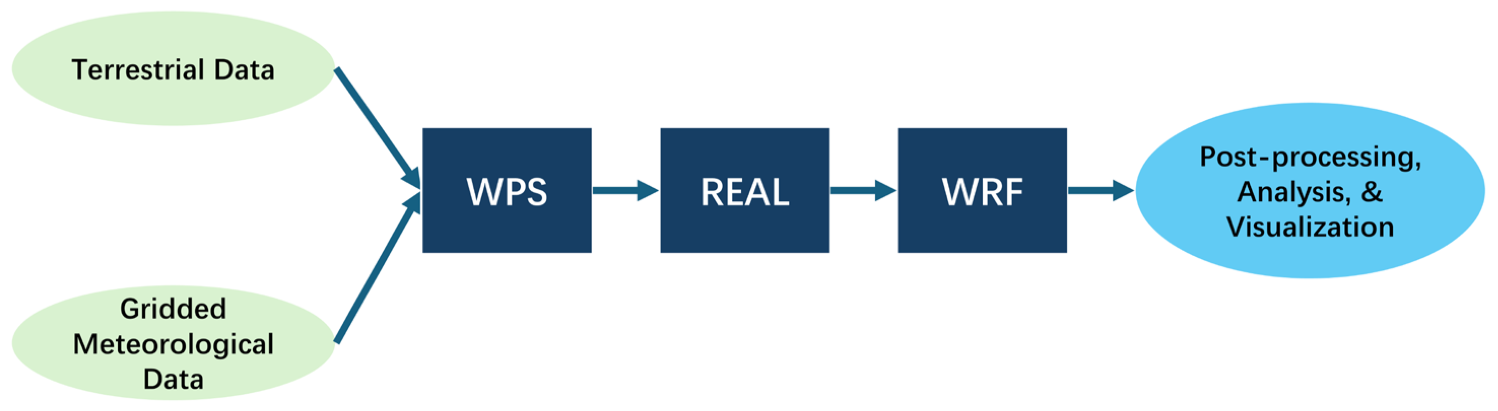
2.1. WRF Model

The Weather Research and Forecasting (WRF) model is an advanced mesoscale numerical weather prediction system designed to support both atmospheric research and operational forecasting applications [33]. Developed collaboratively by the National Center for Atmospheric Research (NCAR), the National Oceanic and Atmospheric Administration (NOAA), and other partners, the WRF model features a highly modular, parallelized, and layered design. It employs a fully compressible, non-hydrostatic model and is equipped with a sophisticated 3D variational data assimilation system and a diverse array of internal parameterization schemes, enabling it to simulate meteorological processes across scales from tens of meters to thousands of kilometers. The fundamental equations of the WRF model are derived from the equations of motion, continuity, state, thermodynamics, and moisture. These are obtained by introducing potential energy and potential temperature into the foundational Navier–Stokes equations and applying terrain-following coordinate transformations. The WRF model utilizes an Arakawa C-grid for horizontal discretization, eta coordinates for vertical levels, and a Runge–Kutta algorithm for time integration.

The WRF workflow, as shown in Figure 1, follows these main steps: (1) The terrestrial data and gridded meteorological data are processed through WRF Preprocessing System (WPS) to interpolate the data onto the grid points of the simulation domain specified by the user; (2) Then, the data are processed using the Initialization program (REAL) to interpolate the meteorological field data onto the vertical layers defined by the user, while also generating the boundary conditions and initial field data; (3) The WRF-ARW Solver (WRF) model is employed to perform time integration of the simulation, resulting in the final simulation output files; (4) Post-processing, analysis, and visualization operations are conducted on the simulation results.

2.2. Empirical Parametric Typhoon Models

The Holland Typhoon Model is an empirical parametric model developed by Greg Holland [12]. Building on Schloemer’s exponential pressure distribution model, Holland introduced the “B parameter” and based the model on the gradient wind field to simulate the wind speed and pressure distribution within a typhoon. The equations for pressure and wind fields in the Holland model are as follows [12]:

$$p\left(r\right)=p_c+(p_n-p_c)(-{\displaystyle \frac{R_{max}}{r}}{)}^B$$

(1)

$$V_g\left(r\right)=\sqrt{(p_n-p_c){\displaystyle \frac{B}{{\rho }_a}}({\displaystyle \frac{R_{max}}{r}}{)}^B\mathit{exp}(-{\displaystyle \frac{R_{max}}{r}}{)}^B+({\displaystyle \frac{rf}{2}}{)}^2}-{\displaystyle \frac{rf}{2}}$$

(2)

In these equations, $p_c$ (hPa) represents the central pressure of the typhoon, and $p_n$ (hPa) is the ambient pressure outside the typhoon, set to 1013.15 hPa in this study. $R_{max}$ (m) is the radius of maximum wind speed, ${\rho }_a$ (kg/m³) denotes air density (set to 1.205 kg/m³), and $f$ (rad/s) is the Coriolis parameter.

$R_{max}$ and $B$ are two key parameters in the Holland model, determining the distribution of the wind field. In this study, the parameters $R_{max}$ and $B$ are determined using formulas derived from Chen Dewen’s work [34]. The formula for $R_{max}$ is based on a fitting analysis conducted for the Northwest Pacific, while the parameter $B$ is referenced from Willoughby et al.’s statistical results [35] and Jakobsen et al.’s comparative analysis across different sea regions [36]. The specific formulas are as follows [34]:

$$R_{max}=69.52\mathit{exp} (-0.0136V_{max})$$

(3)

$$B=\left\{\begin{array}{c}0.606+0.0177V_{max}+0.0094\Phi V_{max}\le 40(m/s)\\ 1.314+0.00895\left(V_{max}-40\right)+0.0094\Phi V_{max}>40(m/s)\end{array}\right.$$

(4)

$V_{max}$ (m/s) represents the maximum wind speed, and $\Phi$ (rad) denotes the latitude.

The formula for the translation wind field is as follows [13]:

$$V_s=\left\{\begin{array}{c}{V}_{sm}{\displaystyle \frac{r}{R_{max}+r}} (0<r\le R_{max})\\ V_{sm}{\displaystyle \frac{R_{max}}{R_{max}+r}} (r>R_{max})\end{array}\right.$$

(5)

In this equation, $V_{sm}$ (m/s) represents the translational velocity of the typhoon center.

The Jelesnianski typhoon model is derived by superimposing a circularly symmetric typhoon wind field with the typhoon translation wind field. The Jelesnianski model exists in two versions: Jelesnianski-1 and Jelesnianski-2 [13,37]. The primary distinction between these two versions lies in the method of constructing the wind profile. In this study, the Jelesnianski-2 version was utilized. The Jelesnianski-2 model is a wind field model that employs a single function to describe the wind profile of a typhoon, which helps to avoid the discontinuity issues near the maximum wind speed that are present in some other models. The circularly symmetric wind field is described as follows [13]:

$$\begin{gathered} \overrightarrow{V_r}=V_{max}{\displaystyle \frac{2\left(r/R_{max}\right)}{1+(r/R_{max}{)}^2}}(A^{\ast }\overrightarrow{i}+B^{\ast }\overrightarrow{j}) \\ {A}^{\ast }=-{\displaystyle \frac{y\mathit{cos}\theta +x\mathit{sin}\theta }{r}} \\ {B}^{\ast }={\displaystyle \frac{x\mathit{cos}\theta -y\mathit{sin}\theta }{r}} \\ r=\sqrt{x^2+y^2} \end{gathered}$$

(6)

In this equation, $\theta$ (°) represents the inflow angle, set to 30° in this study; $r$ (m) is the distance from the calculation point to the center of the typhoon; $\overrightarrow{i}$ and $\overrightarrow{j}$ are the unit vectors in the x and y directions, respectively.

The formula for calculating the translation wind field is consistent with the one used in the Holland model.

2.3. SWAN Model

The SWAN model is the third-generation numerical model for nearshore waves, designed to simulate the wave dynamics in shallow water regions such as coasts and estuaries. Developed and maintained by Delft University of Technology in the Netherlands, the core of the SWAN model is based on the action balance equation. It can incorporate various physical processes, including wave propagation, refraction, shoaling, breaking, and nonlinear wave–wave interactions. Additionally, the SWAN model employs a fully implicit finite difference scheme, which provides greater flexibility in time step selection, allowing the model to remain stable even in shallow water regions.

The SWAN model employs the action balance equation to describe the governing equation for waves. In Cartesian coordinates, the equation is expressed as follows [38]:

$${\displaystyle \frac{\partial }{\partial t}}N+{\displaystyle \frac{\partial }{\partial x}}{C}_{x}N+{\displaystyle \frac{\partial }{\partial y}}{C}_{y}N+{\displaystyle \frac{\partial }{\partial \sigma }}{C}_{\sigma }N+{\displaystyle \frac{\partial }{\partial \theta }}{C}_{\theta }N={\displaystyle \frac{S}{\sigma }}$$

(7)

In this equation, $N$ (m₂/s) is the evolution of the action density; t (s) is time; $C_x$ (m/s) and $C_y$ (m/s) are the propagation velocities of wave energy in the x and y directions, respectively; $C_{\sigma }$ (m/s) and $C_{\theta }$ (m/s) are the propagation velocities in spectral spaces $\sigma$ and $\theta$, respectively; and $S$ represents the energy source.

In the SWAN model, the energy source can be represented as follows [38]:

$$S=S_{in}+S_{ds,w}+S_{ds,b}+S_{ds,br}+S_{nl3}+S_{nl4}$$

(8)

In this equation, $S_{in}$ represents the wind energy input term, $S_{ds,w}$ denotes the whitecap dissipation term, $S_{ds,b}$ is the bottom friction dissipation term, $S_{ds,br}$ corresponds to the wave-breaking dissipation term, $S_{nl3}$ signifies the triad wave–wave interaction term, and $S_{nl4}$ is the quadruplet wave–wave interaction term.

2.4. Data Description

In this study, the WRF model is driven by both FNL and ERA5 datasets, and the CMA data are used to drive the Holland and Jelesnianski models. Then, the results are compared with the typhoon wind speed data recorded by the SMAP.

Table 1. The datasets used in the study.

Dataset Name	Usage	Description
FNL	The dataset used to drive the WRF model	FNL data are on 1-degree by 1-degree grids prepared operationally every six hours, and can be downloaded from https://rda.ucar.edu/datasets/d083002/ (accessed on 1 October 2024) [39].
ERA5	The dataset used to drive the WRF model	ERA5 data are on 0.25-degree by 0.25-degree grids prepared operationally every hour and can be downloaded from https://cds.climate.copernicus.eu/datasets (accessed on 1 October 2024) [40].
SMAP	Actual observational dataset	Each SMAP file consists of two 0.25° gridded daily maps of wind speeds, the wind speed data at a 10 m height above the sea surface is obtained through the L-band radiometer onboard the SMAP satellite and can be downloaded from https://remss.com/missions/SMAP/winds/ (accessed on 1 October 2024) [41].
CMA	Actual observational dataset	CMA dataset provides the position and intensity of tropical cyclones in the Northwest Pacific (including the South China Sea, north of the equator, and west of 180°E) every 6 h since 1949, can be downloaded from https://tcdata.typhoon.org.cn/zjljsjj.html (accessed on 1 October 2024) [42,43].

provides descriptions of the datasets used in this study. It should be noted that the CMA dataset in this study has been linearly interpolated to a 1 h time interval.

3. Simulation Scheme Description

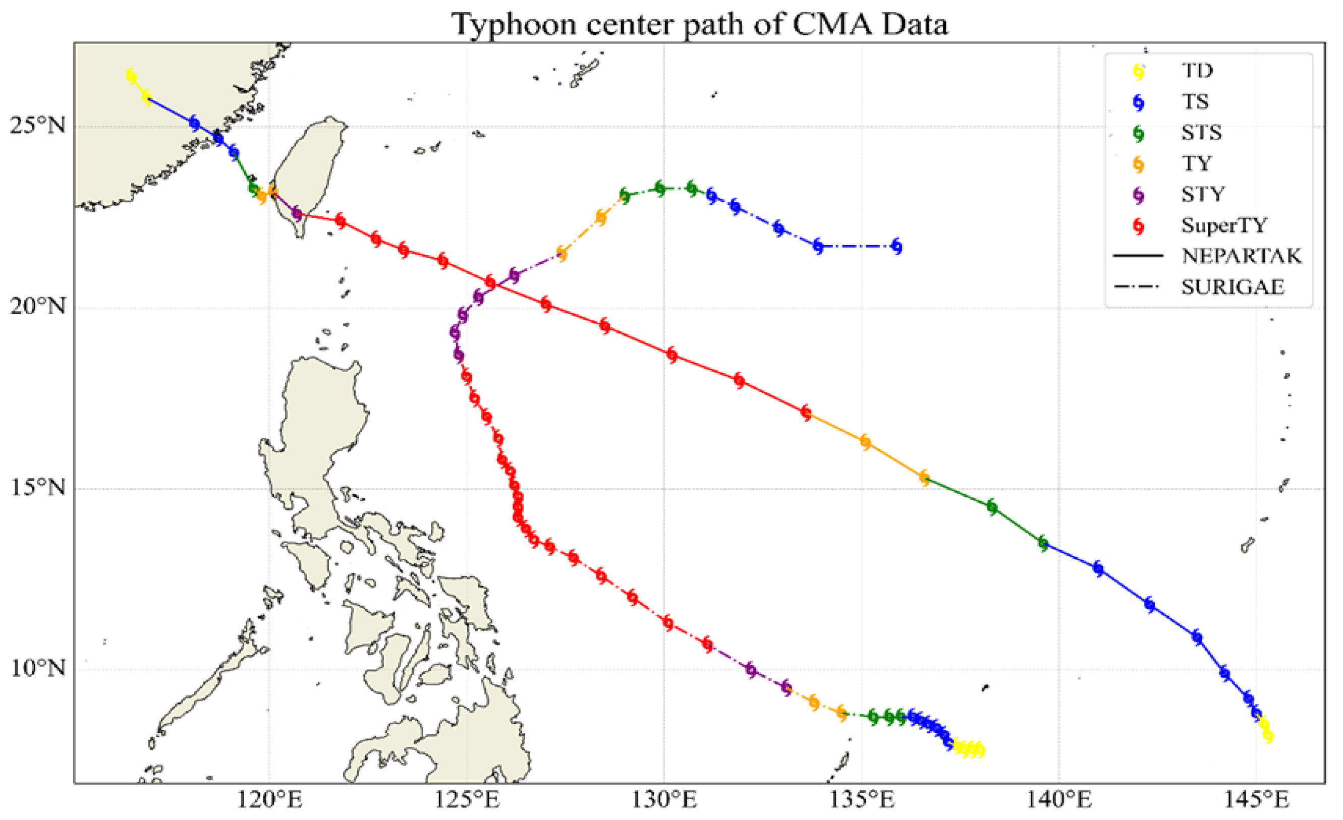
3.1. Typhoon Description

This study simulates Typhoon Surigae (2102) and Typhoon Nepartak (1601). The following are the basic details of these two typhoons:

Typhoon Surigae developed east of the Philippines on 14 April 2021, and rapidly intensified, reaching super typhoon strength by 17 April. On the morning of 18 April, it reached its peak intensity, with the maximum wind speed near the center exceeding 68 m per second, corresponding to a force of 17 on the Beaufort scale, and the minimum central pressure dropping to approximately 905 hPa. This made it the strongest tropical cyclone ever recorded in April globally. Typhoon Nepartak originated south of Guam, USA, on 3 July 2016, and rapidly intensified, reaching the strength of a super typhoon within 24 h from a tropical storm. Guided by the subtropical high-pressure ridge, Nepartak moved northwest at a relatively fast pace, making landfall in Taitung County, Taiwan, at 5:50 AM on 8 July 2016, as a super typhoon. The typhoon brought severe winds and heavy rainfall to Taiwan, causing significant damage and casualties. Figure 2 shows the tracks and intensity information of the two typhoons, as recorded by the CMA dataset.

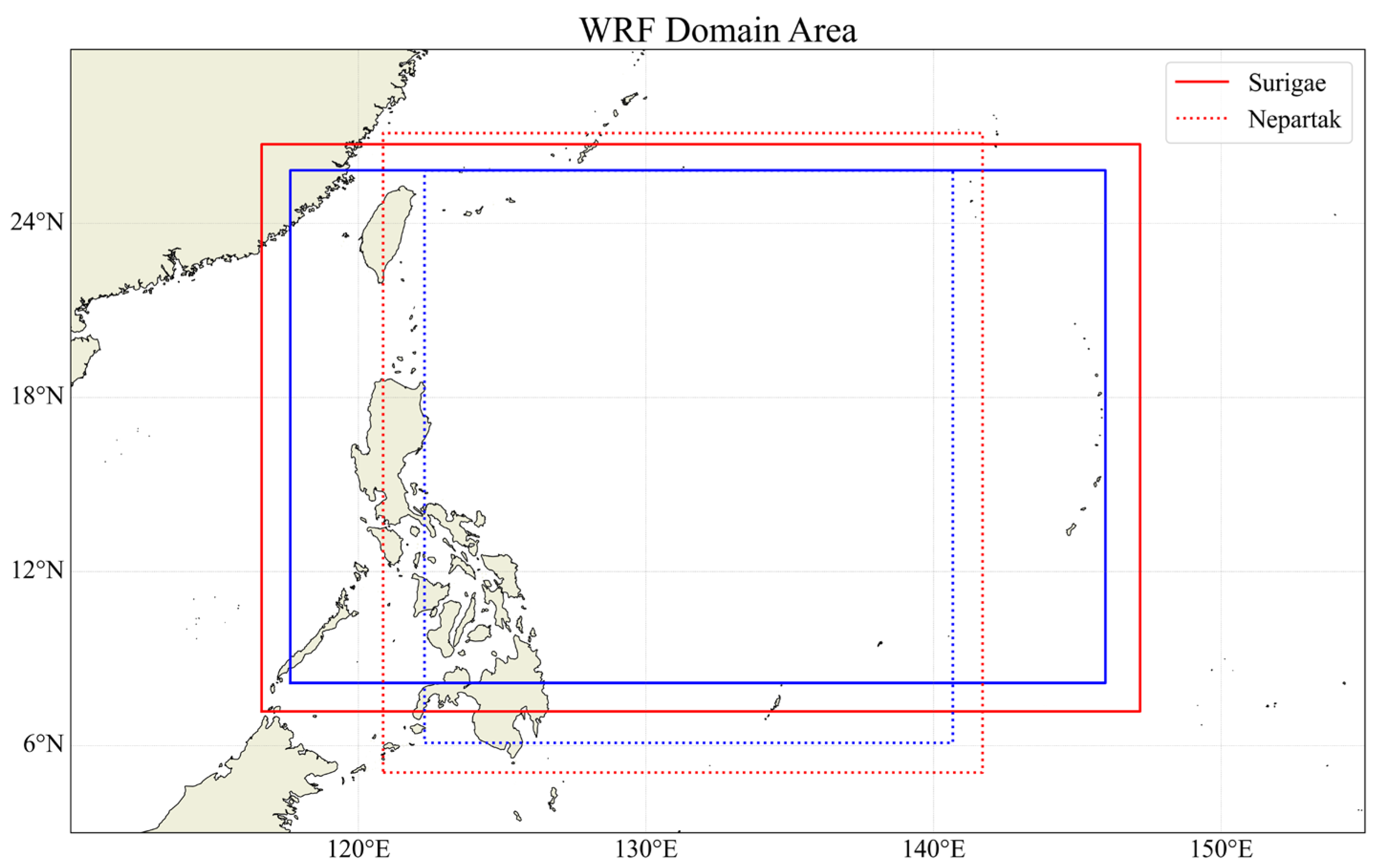
3.2. WRF Scheme Description

The version of the WRF model used in this study is 4.6.1, with the ARW core. A two-way nested scheme with two layers is applied for the WRF simulations, with resolutions set to 21 km and 7 km. The time step is set to 120 s, and the reanalysis data driving the WRF model are ERA5 and FNL. Figure 3 shows the simulation domains for Typhoon Surigae and Typhoon Nepartak. The simulation period for Typhoon Surigae is from 00:00 UTC on 13 April 2021, to 00:00 UTC on 26 April 2021. The simulation period for Typhoon Nepartak is from 00:00 UTC on 2 July 2016, to 00:00 UTC on 10 July 2016. The main parameter settings for the WRF simulations of the typhoons are summarized in

Table 2. Main parameter settings for WRF simulations.

Namelist Parameter	Setting Codes	Description
mp_physics	24, 24	WSM7
ra_lw_physics	1, 1	RRTM
ra_sw_physics	1, 1	Dudhia
sf_sfclay_physics	1, 1	revised MM5 Monin–Obukhov
sf_surface_physics	2, 2	unified Noah
bl_pbl_physics	1, 1	YSU
cu_physics	1, 1	Kain–Fritsch (new Eta)
sf_ocean_physics	1	simple ocean mixed layer (oml) model
isftcflx	1	Donelan Cd + constant Z0q for Ck

.

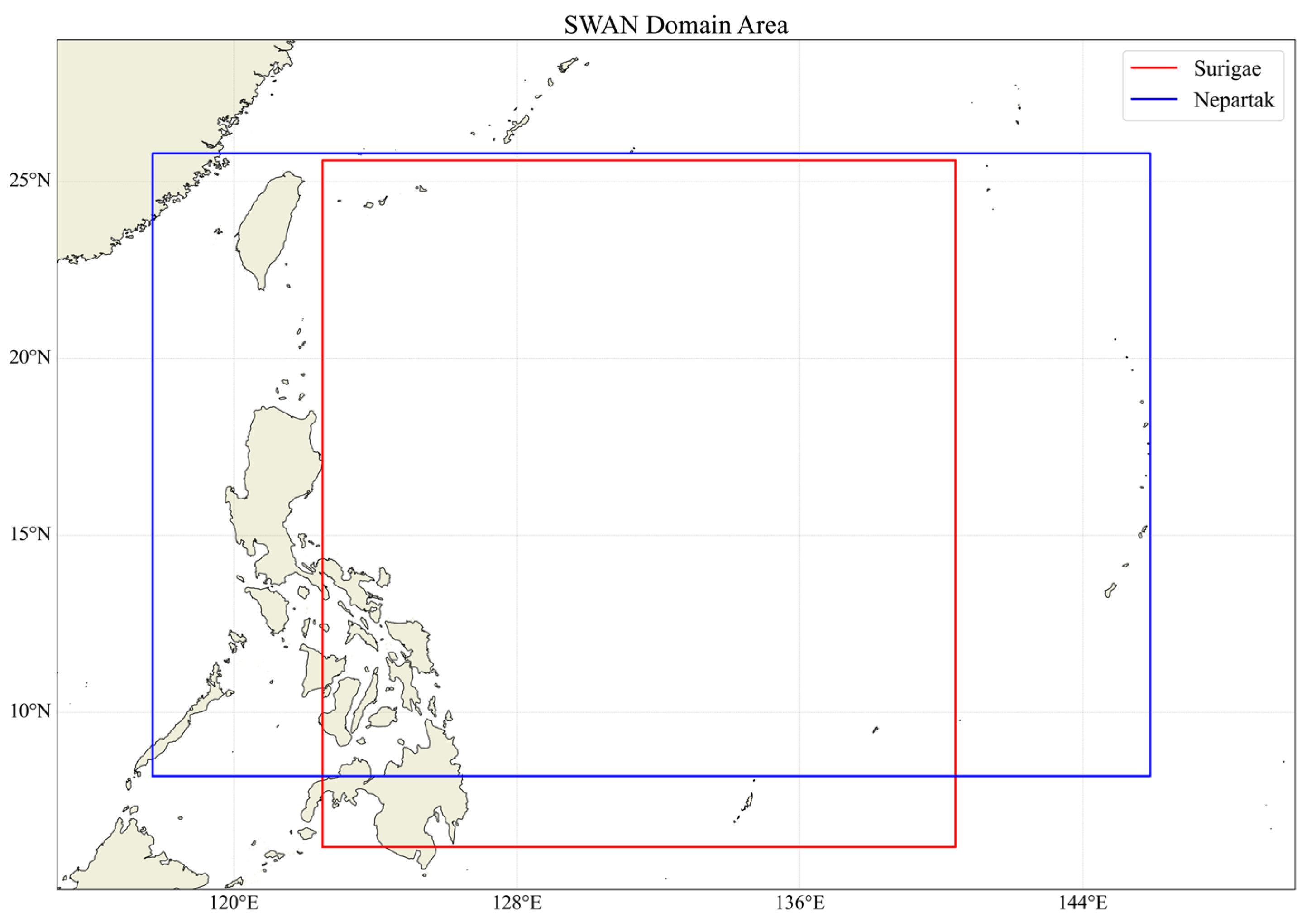
3.3. Description of the SWAN Scheme

The SWAN model uses a structured grid, with a grid resolution set to 0.1°, and a time step of 10 min. The simulation period aligns with that of the WRF model, with effective wave height data output every hour. Figure 4 shows the SWAN simulation domains for Typhoon Surigae and Typhoon Nepartak. The driving wind field for the SWAN model will use wind field data from both the WRF simulations and the empirical parameter typhoon models. The “cubic” interpolation method is employed to interpolate the wind speed data to the SWAN simulation domain. The bathymetry data used in the SWAN simulations come from the ETOPO1 global topographic elevation dataset, published by the National Geophysical Data Center (NGDC) of the United States.

4. Results

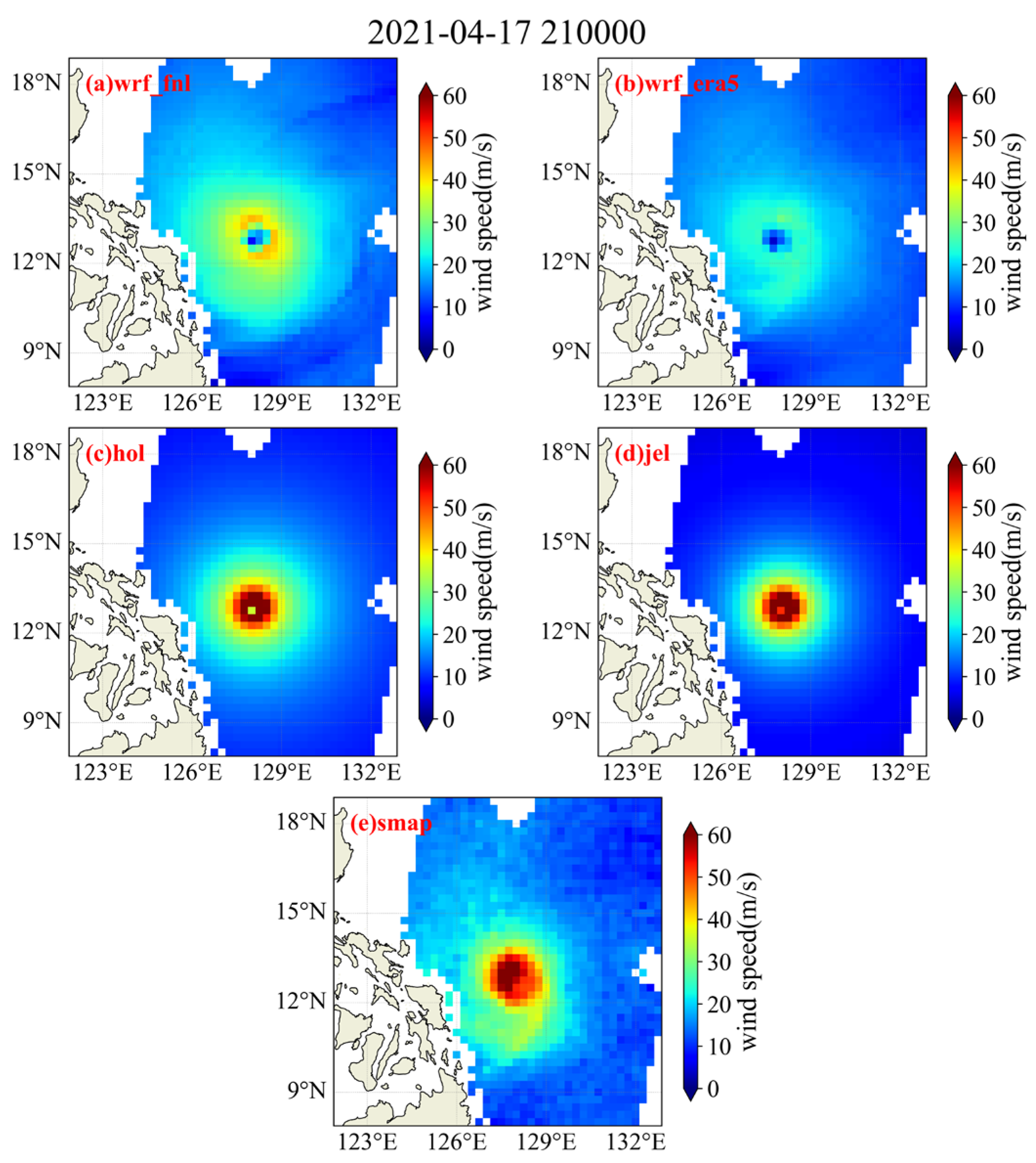
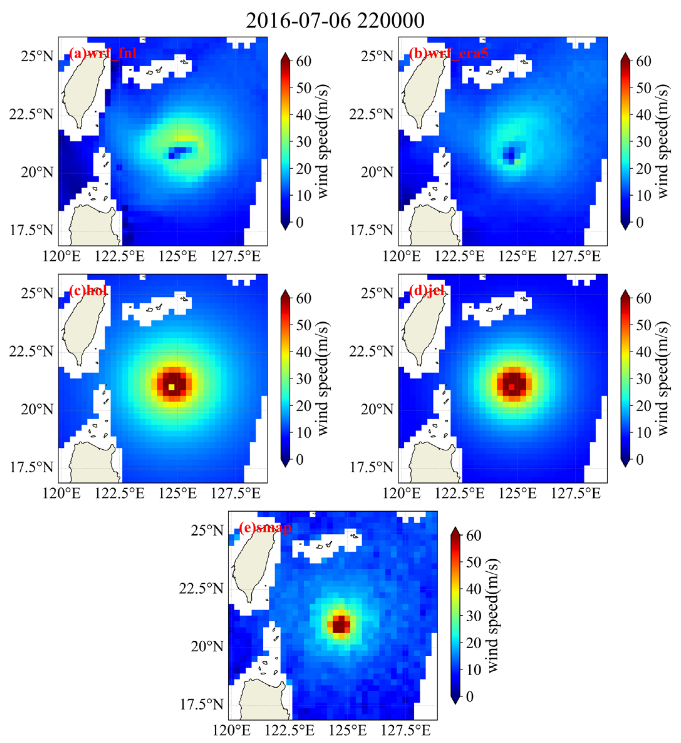
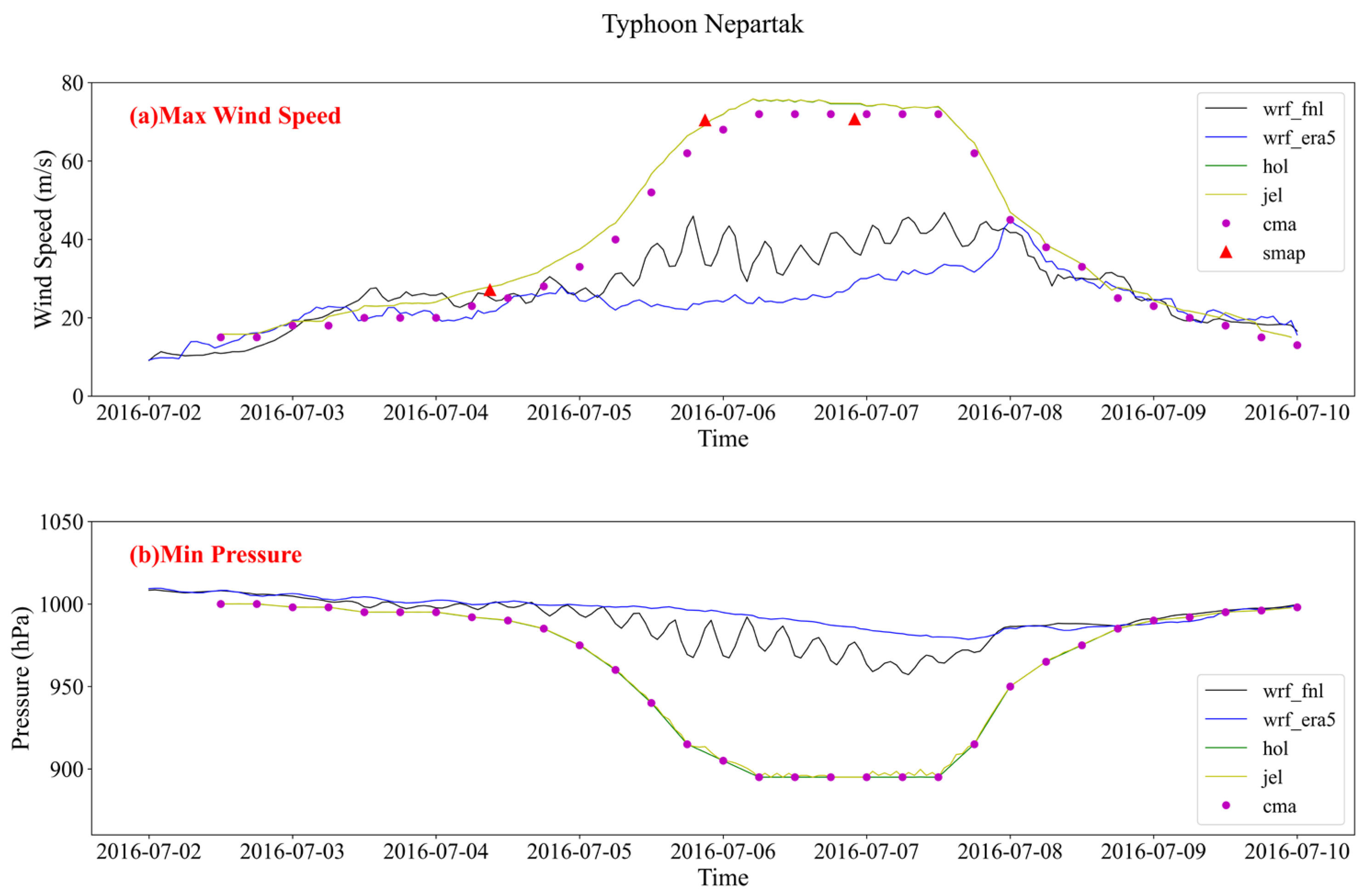
4.1. Evaluation of Simulated Typhoon Wind Speed

The wind speed data from the WRF and empirical parameter typhoon models are compared with the SMAP wind speed data. To ensure consistency in the comparison, the simulated data from the WRF and empirical parameter typhoon models are interpolated and masked according to the SMAP wind field data.

Table 3. Abbreviations used in the figures and descriptions.

Abbreviation	Description
wrf_fnl	The WRF simulation results driven by FNL data
wrf_era5	The WRF simulation results driven by ERA5 data
hol	The simulation results of the Holland model
jel	The simulation results of the Jelesnianski model
smap	The SMAP wind field data
CMA	The CMA tropical cyclone’s best track data

provides explanations for the corresponding cases where abbreviations are used in the presentation of results.

Figure 5 and Figure 6 display the comparison of simulation results for Typhoon Surigae with SMAP data. From Figure 5 and Figure 6, it can be observed that the highest wind speed recorded by SMAP always exceeds 60 m/s. However, the wind speed simulated by WRF driven by FNL and ERA5 data peaks around 40 m/s, showing a certain discrepancy with the extreme wind speeds observed by SMAP. The empirical parameter typhoon models, Holland and Jelesnianski, provide wind speed extremes that are closer to the SMAP wind speed data compared to the WRF simulations, with both models simulating peak wind speeds reaching 60 m/s. However, the simulated wind speeds outside the typhoon’s influence area of WRF simulations are closer to the SMAP wind field data.

Therefore, it can be inferred that, compared to the WRF model, the empirical parameter typhoon models, Holland and Jelesnianski, have an advantage in simulating the intensity of the typhoon. However, they are less effective than the WRF model in simulating the wind field in the outer regions of the typhoon and the structure of the Typhoon. It is noteworthy that the extreme wind speed data simulated by the WRF model driven by ERA5 is lower than that simulated by the WRF model driven by FNL.

Figure 7 and Figure 8 present the comparison of Typhoon Nepartak, with data uniformly interpolated and masked. As shown in Figure 7, the typhoon was in a strong tropical storm stage, with the maximum wind speed reaching approximately 30 m/s. At this point, there was little difference in the maximum wind speed simulation between the WRF model and the empirical parameterized typhoon models. However, in the region outside of the typhoon, the WRF simulated wind field data were found to be more consistent with the SMAP data.

In Figure 8, which corresponds to the times of 6 July 2016, 22:00, the typhoon had intensified to a super typhoon with maximum wind speeds exceeding 60 m/s. The empirical parameterized typhoon models, Holland and Jelesnianski, demonstrated better agreement with the SMAP wind field data in terms of maximum wind speed simulation compared to the WRF model simulations driven by FNL and ERA5 data.

For the simulation of Typhoon Nepartak, the maximum wind speeds simulated using ERA5-driven WRF were consistently lower than those obtained using FNL-driven WRF, which aligns with the findings for Typhoon Surigae. On 6 July 2016, at 22:00, the maximum wind radius simulated by the empirical parameterized typhoon model Jelesnianski was found to be closer to the SMAP data compared to the Holland model. The Holland model tends to overestimate the high wind speed regions of the typhoon.

Regarding the WRF simulations, the use of FNL data for model driving resulted in stronger wind speeds compared to simulations driven by ERA5 data. This demonstrates that the choice of driving data significantly influences the wind speed simulations in WRF and using more accurate and realistic driving data can enhance the performance of wind speed predictions in the WRF model.

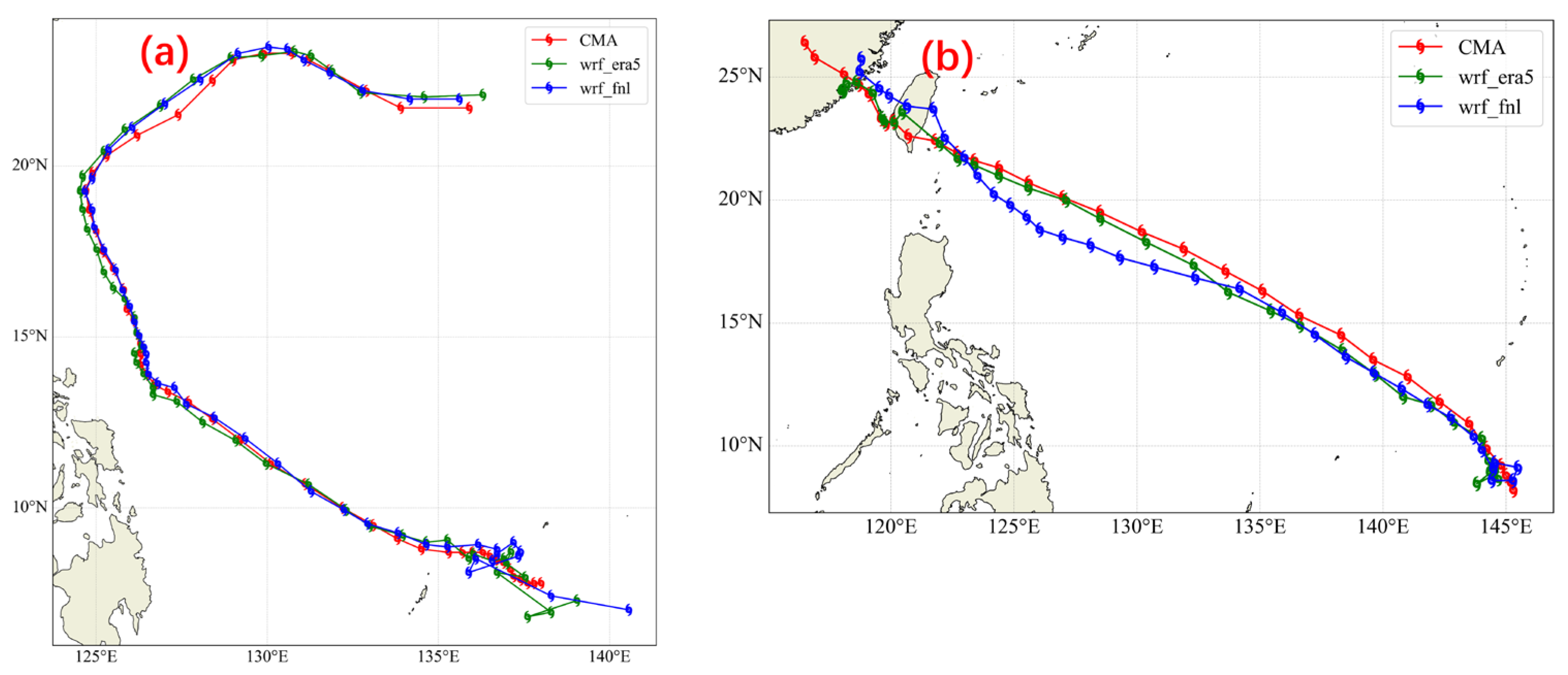
4.2. Typhoon Center Path Compare

The sea-level pressure (SLP) data extracted from the WRF simulation results were used to determine the typhoon center by identifying the minimum SLP value. This center location was then compared with data from the CMA data, as shown in Figure 9. The red line represents CMA data, while the blue and green lines correspond to WRF simulations driven by FNL and ERA5 datasets, respectively.

At the early stages of the WRF simulation, when the typhoon was still in the tropical depression or tropical storm phase, its structure had not fully formed. Consequently, determining the typhoon center based on the minimum SLP showed some variability. However, as the typhoon intensified, the central position extracted by this method increasingly aligned with CMA data. For the Typhoon Surigae simulation, both ERA5- and FNL-driven WRF simulations yielded typhoon tracks that closely matched CMA data, demonstrating overall accuracy. For Typhoon Nepartak, however, the ERA5-driven simulation provided a track that more accurately reflected CMA data than the FNL-driven simulation.

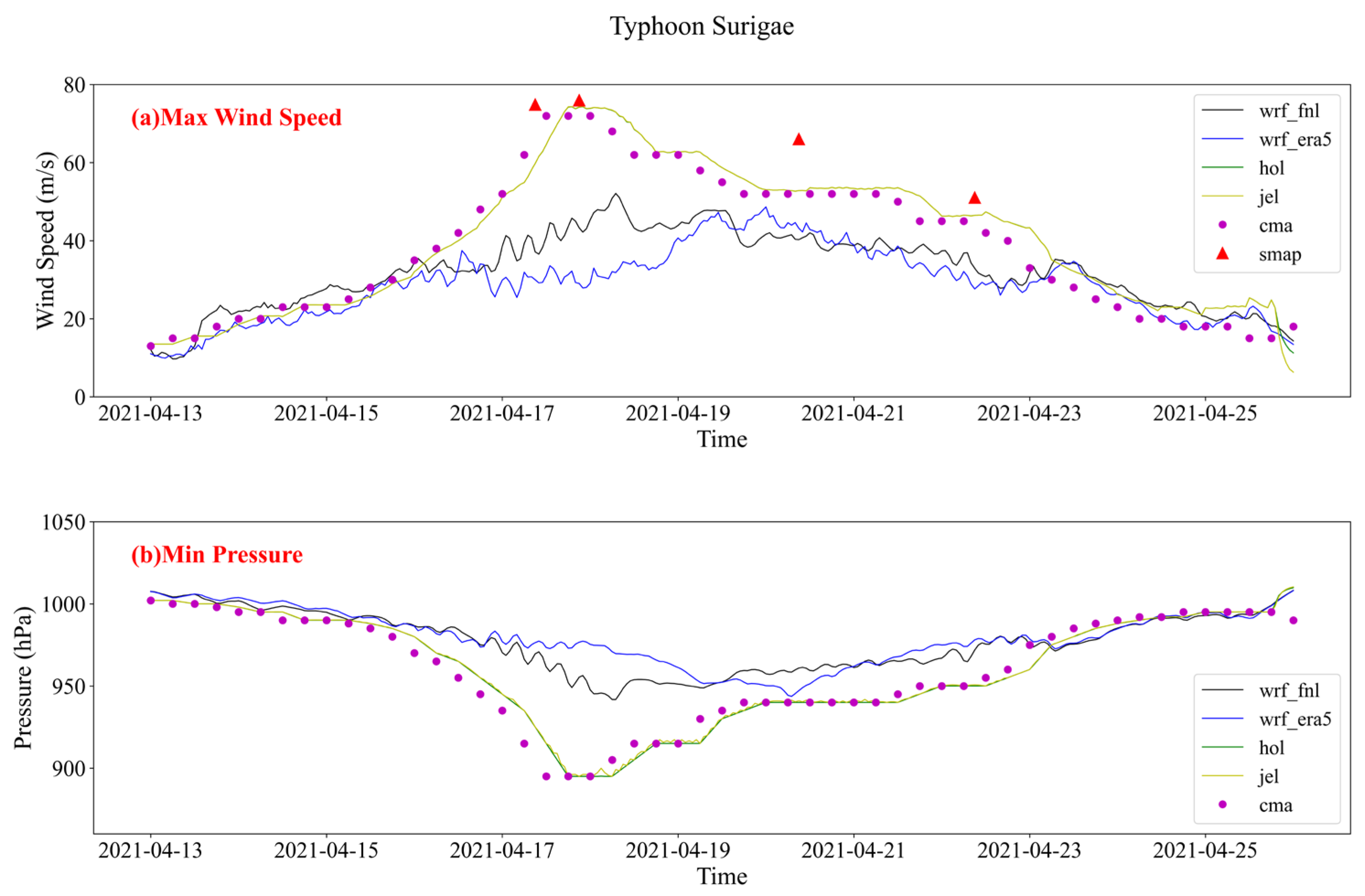
4.3. Comparison of Typhoon Intensity Simulations

A comparison is made between the extreme wind speeds from SMAP data, WRF simulations driven by FNL and ERA5, and the empirical parameterized typhoon models, Holland and Jelesnianski, as shown in Figure 10 and Figure 11. Subfigure (a) of Figure 10 presents the comparison of extreme wind speeds for Typhoon Surigae. The SMAP extreme wind speeds are generally higher than those recorded by the CMA. The empirical parameterized typhoon models, Holland and Jelesnianski, match the CMA data more closely, whereas the extreme wind speed simulations from WRF driven by FNL and ERA5 deviate significantly from CMA data. In the simulation of typhoon extreme wind speed, the results from the empirical parameterized typhoon models Holland and Jelesnianski are nearly identical. Specifically, from 17 April to 19 April 2021, the FNL-driven WRF simulation provides a better match to the extreme wind speeds compared to the ERA5-driven simulation, although neither simulation reaches the typhoon intensity recorded by the CMA during the rapid intensification phase.

Subfigure (b) of Figure 10 compares the minimum surface pressure. Similarly, the empirical parameterized typhoon models, Holland and Jelesnianski, provide simulations that are closer to the CMA data than the WRF simulations driven by FNL and ERA5. However, during the rapid intensification phase of the typhoon, the minimum surface pressures simulated by both empirical parameterized models are slightly higher than those recorded by the CMA.

Figure 11 shows the intensity simulation for Typhoon Nepartak. Unlike Typhoon Surigae, the extreme wind speed simulated by the empirical parameterized typhoon model Jelesnianski is generally slightly higher than the CMA recorded data. For surface pressure, both the empirical parameterized typhoon models, Holland and Jelesnianski, align well with the CMA data. In contrast, the simulations of WRF driven by FNL and ERA5 deviate significantly from the CMA data.

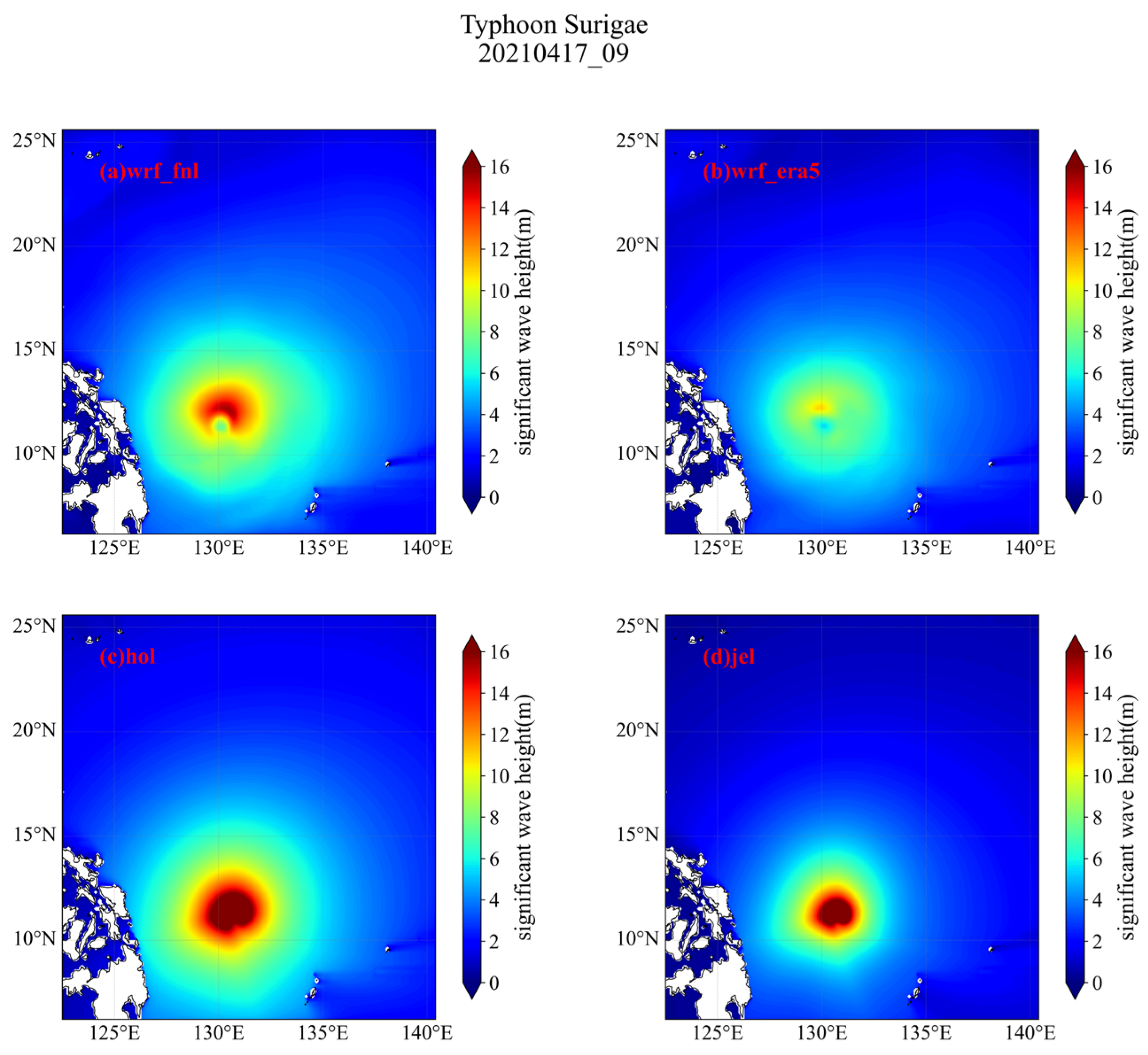
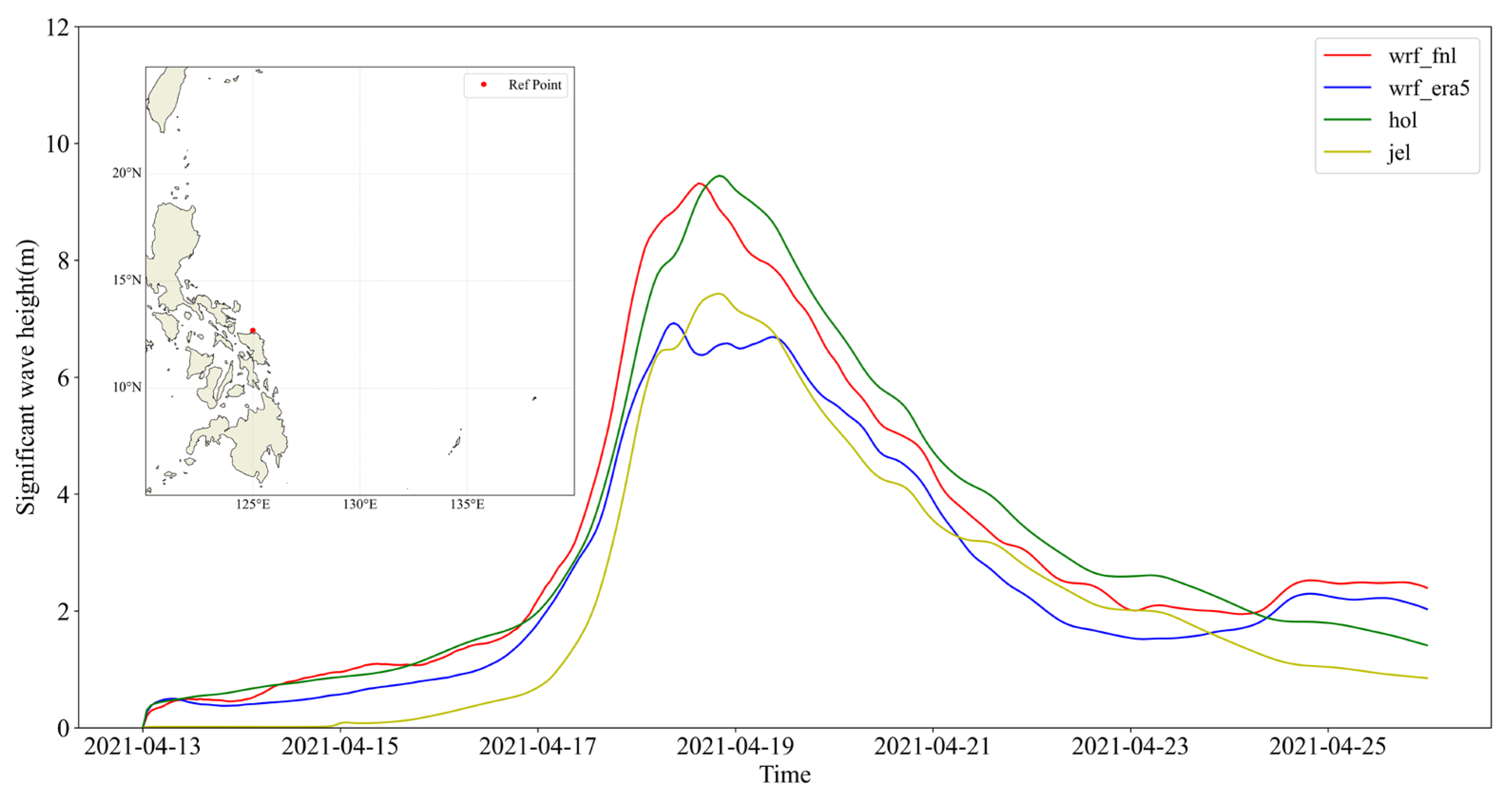
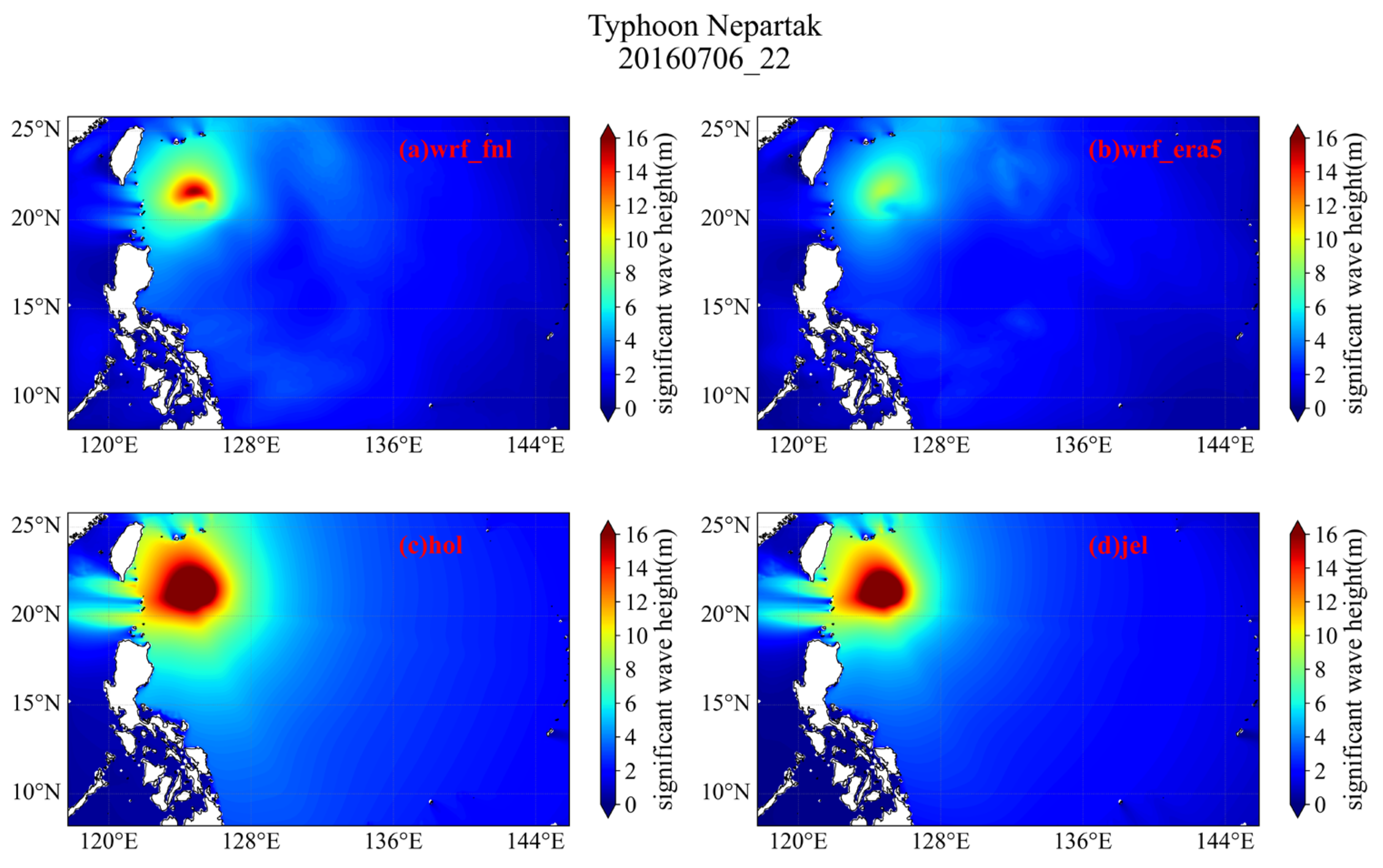
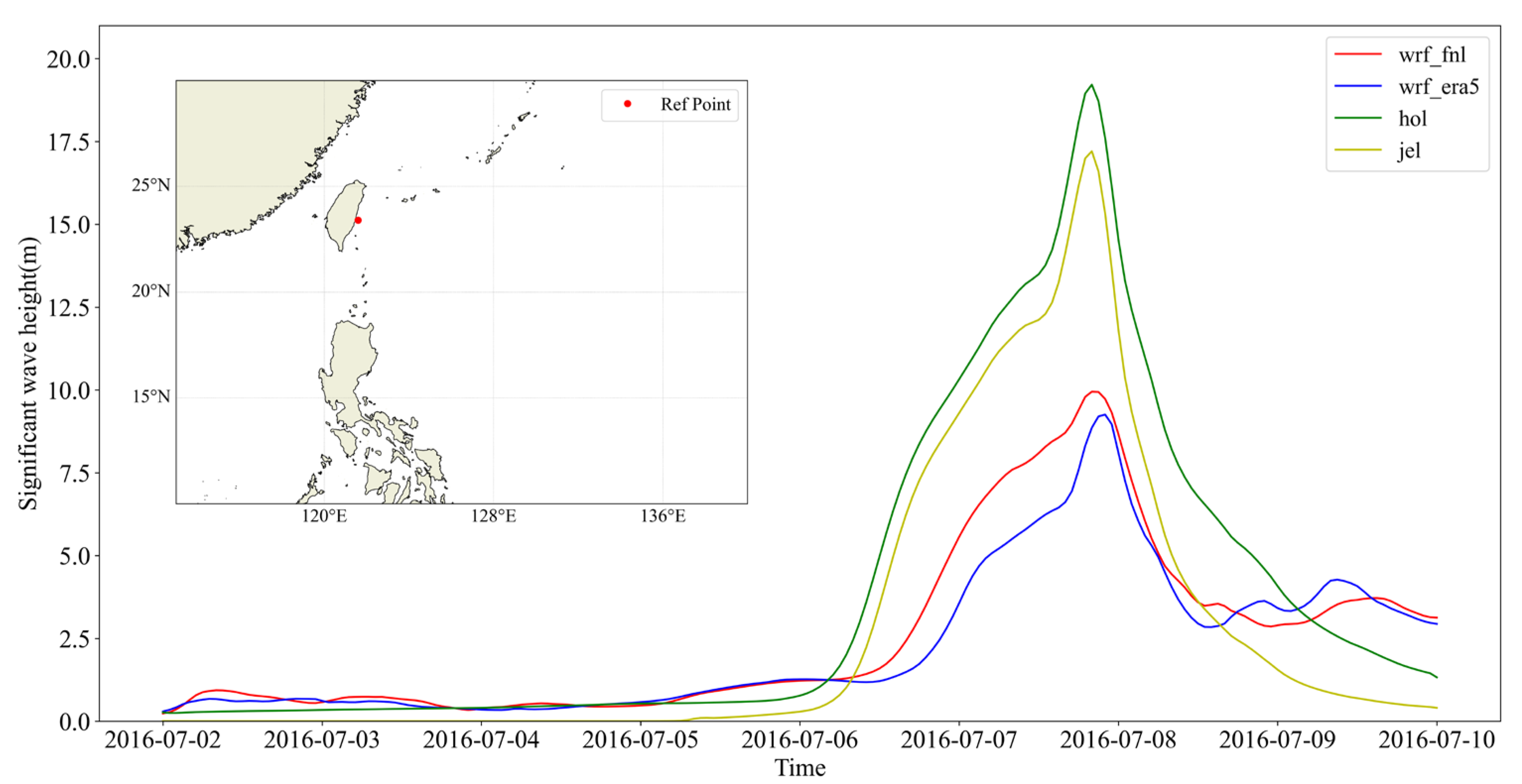
4.4. Significant Wave Height Results from SWAN

The wind field data at a height of 10 m from the empirical parameterized typhoon models Holland and Jelesnianski, as well as from WRF simulations driven by FNL and ERA5, were used as the input wind fields for the SWAN model. The significant wave height data within the simulation domain were then output.

Figure 12 presents a comparison of the significant wave height simulations in Typhoon Surigae. From the figure, it is evident that, except for the ERA5-driven WRF simulation, the extreme values of the significant wave height reached 16 m. However, the range of extremely significant wave height values from the empirical parameterized typhoon models, Holland and Jelesnianski, was higher than that from the FNL-driven WRF simulation, which is consistent with the earlier wind field comparison.

A reference point was then selected to extract the time series of significant wave height at this location. Figure 13 shows the location of the reference point near the coast, and the time series of significant wave height at this point. As shown in Figure 13, between 00:00 on 13 April 2021, and 00:00 on 18 April 2021, the significant wave height simulations are relatively consistent across all cases except for the Jelesnianski model. This can be attributed to the smaller radius of maximum wind speed in the Jelesnianski model compared to the Holland model, as observed in the previous wind field comparisons. Since the reference point is located farther from the typhoon’s center, the wind field simulated by the Jelesnianski model at this location is weaker. Between 00:00 on 18 April 2021, and 00:00 on 19 April 2021, the maximum significant wave height exceeded 8 m in simulations using the FNL-driven WRF model and the Holland model, whereas it remained below 8 m in cases driven by ERA5 and the Jelesnianski model. This difference is likely due to the lower typhoon wind speeds produced by the ERA5-driven WRF simulation compared to the FNL-driven WRF simulation. Additionally, since the reference point is far from the typhoon’s center, the WRF model’s advantage in simulating peripheral wind fields becomes predominant. Consequently, the significant wave height simulated using FNL-driven WRF surpasses that of the Jelesnianski model.

Figure 14 shows the significant wave height output from SWAN for Typhoon Nepartak. The distribution of significant wave height from the empirical parameterized typhoon models, Holland and Jelesnianski, differs significantly. The high-value range of significant wave height simulated by the Holland model is larger compared to the Jelesnianski model. This discrepancy is related to the radius of maximum wind speed of the typhoon. From the wind speed comparison in Figure 8, it is evident that the radius of maximum wind speed simulated by Jelesnianski is smaller than that of the Holland model, which contributes to the difference in significant wave height distribution. For the WRF simulations, the wind speeds simulated using ERA5 are lower than those simulated using FNL. Consequently, in the comparison of significant wave height, the extreme values from the FNL-driven simulation are higher than those from the ERA5-driven simulation.

A reference point was selected to extract the time series of significant wave heights. Figure 15 presents the simulation results for Typhoon Nepartak. Throughout the entire time series, the significant wave height at the reference point simulated by the Holland empirical parameterized typhoon model is consistently higher than that of the Jelesnianski model. This is similarly attributed to the smaller maximum wind radius range in the Jelesnianski model compared to the Holland model. Additionally, the peak significant wave heights simulated by both the Holland and Jelesnianski models are noticeably higher than those simulated using FNL- and ERA5-driven WRF. This is because the reference point is closer to the typhoon’s central path, where the advantage of empirical parameterized typhoon models in simulating extreme wind speeds becomes dominant.

5. Discussion and Conclusions

5.1. Discussion

Empirical parameterized typhoon models demonstrate superior performance in simulating typhoon maximum wind speeds compared to the WRF model. This advantage arises from their direct use of critical typhoon information, such as maximum wind speed, during the computation process, enabling these models to closely replicate maximum wind speeds in CMA data. In contrast, the WRF model is constrained by the grid resolution of reanalysis datasets, such as FNL and ERA5. The maximum wind speed may occur between grid points, resulting in an attenuation of extreme wind speeds in the simulated data. Furthermore, the level of refinement and accuracy of the reanalysis of the driving fields significantly influences the WRF model’s outputs. Therefore, employing finer and more realistic reanalysis datasets is pivotal for enhancing the WRF model’s simulation performance.

While increasing the resolution of WRF simulations can improve their accuracy, it also imposes significantly higher demands on computational resources. In comparison, empirical parameterized typhoon models require considerably fewer computational resources. However, the WRF model accounts for interactions between the typhoon and its surrounding environment, a feature absent in empirical parameterized typhoon models, which rely solely on empirical formulas to estimate typhoon parameters. Consequently, the WRF model outperforms empirical parameterized typhoon models in simulating wind fields in the outer regions of typhoons.

The experiments revealed that the maximum wind radius simulated by empirical parameterized typhoon models tends to exceed the observations from SMAP data. This discrepancy can result in overestimated wind speeds and significant wave heights in regions slightly farther from the typhoon’s central path. Therefore, careful calibration of the maximum wind radius parameter is crucial to improve the accuracy of these models.

5.2. Conclusions

This study compares two super typhoons (Typhoon Surigae 2021 and Typhoon Nepartak 2016) using four simulation scenarios: (1) FNL-driven WRF model; (2) ERA5-driven WRF model; (3) Holland empirical typhoon model; and (4) Jelesnianski empirical typhoon model. Simulated wind fields were compared with SMAP satellite data, and the models’ accuracy, particularly at high wind speeds, was evaluated. The main findings are:

(1).

The Holland and Jelesnianski models simulate extreme wind speeds (above 50 m/s) better than the WRF model driven by FNL and ERA5 data.

(2).

WRF simulations driven by FNL data perform better in simulating high wind speeds than those driven by ERA5. Additionally, WRF simulates the wind field in the outer regions of the typhoon more accurately than the empirical models.

(3).

The maximum wind radius range simulated by the Holland empirical parameterized typhoon model tends to be overestimated, resulting in higher wind speed and significant wave height simulations at locations closer to the typhoon’s central path. Therefore, parameters such as the maximum wind radius require careful consideration and refinement.

Future research will focus on combining empirical parameterized typhoon models with WRF simulations to achieve a balance between accurately reproducing the typhoon’s core wind speeds and considering the interactions between the typhoon and its surrounding environment. For instance: integrating four-dimensional data assimilation (FDDA) with Observation Nudging into the WRF model to improve extreme wind speed simulations, using unstructured grids in the SWAN model for higher resolution in nearshore areas, and optimizing the maximum wind speed radius in the empirical models to enhance their accuracy. Additionally, attempts to use stochastic methods to simulate typhoon activities around Taiwan and its surrounding areas. By integrating satellite observation data, try to summarize the characteristics of extreme wind speeds associated with typhoons in the Taiwan region.

References

1. Li, X.; Han, G.; Yang, J.; Wang, C. Remote Sensing Analysis of Typhoon-Induced Storm Surges and Sea Surface Cooling in Chinese Coastal Waters. Remote Sens. 2023, 15, 1844. [Google Scholar] [CrossRef]
2. Tang, R.; Shen, F.; Ge, J.; Yang, S.; Gao, W. Investigating typhoon impact on SSC through hourly satellite and real-time field observations: A case study of the Yangtze Estuary. Cont. Shelf Res. 2021, 224, 104475. [Google Scholar] [CrossRef]
3. Yang, C.; Shi, B.; Min, J. The Combination Application of FY-4 Satellite Products on Typhoon Saola Forecast on the Sea. Remote Sens. 2024, 16, 4105. [Google Scholar] [CrossRef]
4. Chen, X.-Z.; Ma, Y.-L.; Lin, C.-Q.; Fan, L.-L. Assessment of Typhoon Precipitation Forecasts Based on Topographic Factors. Atmosphere 2023, 14, 1607. [Google Scholar] [CrossRef]
5. Zeng, Z.-h.; Chen, L.; Wang, Y.-q. A numerical simulation study of super Typhoon Saomei (2006) intensity and structure changes. Acta Meteorol. Sin. 2009, 67, 750–763. [Google Scholar]
6. Chen, Y.Z.; Zhan, J.M.; Luo, Y.Y.; Wai, O.W.H.; Tang, L. Responses of thermal structure and vertical dynamic structure of South China Sea to Typhoon Chanchu. J. Hydrodyn. 2014, 26, 458–466. [Google Scholar] [CrossRef]
7. Potty, J.; Oo, S.; Raju, P.; Mohanty, U. Performance of nested WRF model in typhoon simulations over West Pacific and South China Sea. Nat. Hazards 2012, 63, 1451–1470. [Google Scholar] [CrossRef]
8. Sunce, L.; Mingfeng, H.; Wenjuan, L.; Wei, L.; Zhibin, X. Numerical simulation of a urban wind field under the influence of typhoon “Mangkhut”. Acta Aerodyn. Sin. 2021, 39, 107–116. [Google Scholar]
9. Wu, Z.; Jiang, C.; Deng, B.; Chen, J.; Liu, X. Sensitivity of WRF simulated typhoon track and intensity over the South China Sea to horizontal and vertical resolutions. Acta Meteorol. Sin. 2019, 38, 74–83. [Google Scholar] [CrossRef]
10. Yang, M.J.; Ching, L. A modeling study of Typhoon Toraji (2001): Physical parameterization sensitivity and topographic effect. Terr. Atmos. Ocean. Sci. 2005, 16, 177–213. [Google Scholar] [CrossRef]
11. Deppermann, C.E. Notes on the origin and structure of Philippine typhoons. Bull. Am. Meteorol. Soc. 1947, 28, 399–404. [Google Scholar] [CrossRef]
12. Holland, G.J. An Analytic Model of the Wind and Pressure Profiles in Hurricanes. Mon. Weather Rev. 1980, 108, 1212–1218. [Google Scholar] [CrossRef]
13. Jelesnianski, C.P. Numerical computations of storm surges without bottom stress. Mon. Weather Rev. 1966, 94, 379–394. [Google Scholar] [CrossRef]
14. Myers, V.A. Characteristics of United States Hurricanes Pertinent to Levee Design for Lake Okeechobee, Florida; US Government Printing Office: Washington, DC, USA, 1954; Volume 30.
15. Wang, L.; Zhang, Z.; Liang, B.; Lee, D.; Luo, S. An efficient method for simulating typhoon waves based on a modified Holland vortex model. J. Mar. Sci. Eng. 2020, 8, 177. [Google Scholar] [CrossRef]
16. Xu, Y.; Wang, Z.F. Response of Surface Ocean Conditions to Typhoon Rammasun (2014). J. Coast. Res. 2017, 80, 92–97. [Google Scholar] [CrossRef]
17. Zhong, X.; Wei, K.; Shang, D.M. An improved azimuth-dependent Holland model for typhoons along the Zhejiang coast prior to landfall based on WRF-ARW simulations. Nat. Hazards 2023, 117, 2325–2346. [Google Scholar] [CrossRef]
18. Wen, Y.F.; Liu, Y.D.; Tan, W.C.; Peng, K.M.; Chen, H.F. The Impact of Horizontal Resolution on the Intensity and Microstructure of Super Typhoon Usagi. J. Trop. Meteorol. 2019, 25, 24–33. [Google Scholar] [CrossRef]
19. Ruan, Z.X.; Li, J.N.; Li, F.Z.; Lin, W.S. Effects of local and non-local closure PBL schemes on the simulation of Super Typhoon Mangkhut (2018). Front. Earth Sci. 2022, 16, 277–290. [Google Scholar] [CrossRef]
20. Xue, G.; Zhang, J.; Chen, H.; Yu, H. Analysis on causes of strengthening of super strong typhoon Saomai (0608) and numerical experiments of the impact of SST on its intensity. Quat. Sci. 2007, 27, 311–321. [Google Scholar]
21. Xu, H.X. A Numerical Study on Impact of Taiwan Island Surface Heat Flux on Super Typhoon Haitang (2005). Adv. Meteorol. 2015, 2015, 710348. [Google Scholar] [CrossRef]
22. Zhang, W.Q.; Zhang, J.L.; Guan, C.L.; Sun, J. Impacts of Surface Exchange Coefficients on Simulations of Super Typhoon Megi (2010) Using a Coupled Ocean-Atmosphere-Wave Model. J. Ocean Univ. China 2023, 22, 587–600. [Google Scholar] [CrossRef]
23. Ou, S.H.; Liau, J.M.; Hsu, T.W.; Tzang, S.Y. Simulating typhoon waves by SWAN wave model in coastal waters of Taiwan. Ocean Eng. 2002, 29, 947–971. [Google Scholar] [CrossRef]
24. Sheng, Y.X.; Shao, W.Z.; Li, S.Q.; Zhang, Y.M.; Yang, H.W.; Zuo, J.C. Evaluation of Typhoon Waves Simulated by WaveWatch-III Model in Shallow Waters Around Zhoushan Islands. J. Ocean Univ. China 2019, 18, 365–375. [Google Scholar] [CrossRef]
25. Shi, Q.; Tang, J.; Shen, Y.M.; Ma, Y.X. Numerical investigation of ocean waves generated by three typhoons in offshore China. Acta Oceanol. Sin. 2021, 40, 125–134. [Google Scholar] [CrossRef]
26. Wu, Y.; Dou, S.T.; Fan, Y.S.; Yu, S.B.; Dai, W.Q. Research on the influential characteristics of asymmetric wind fields on typhoon waves. Front. Mar. Sci. 2023, 10, 1113494. [Google Scholar] [CrossRef]
27. Wang, L.; Wei, X.; Sun, Y.; Jiang, M.; Li, Q. The Wave Numeric Simulation of 0920 Super Typhoon Lupit. Adv. Mar. Sci. 2015, 2, 94–101. [Google Scholar]
28. Wu, Z.; Jiang, C.; Deng, B.; Chen, J.; Cao, Y.; Li, L. Evaluation of numerical wave model for typhoon wave simulation in South China Sea. Water Sci. Eng. 2018, 11, 229–235. [Google Scholar] [CrossRef]
29. Hsiao, S.C.; Chen, H.E.; Wu, H.L.; Chen, W.B.; Chang, C.H.; Guo, W.D.; Chen, Y.M.; Lin, L.Y. Numerical Simulation of Large Wave Heights from Super Typhoon Nepartak (2016) in the Eastern Waters of Taiwan. J. Mar. Sci. Eng. 2020, 8, 217. [Google Scholar] [CrossRef]
30. Mazyak, A.R.; Shafieefar, M. Development of a hybrid wind field for modeling the tropical cyclone wave field. Cont. Shelf Res. 2022, 245, 104788. [Google Scholar] [CrossRef]
31. Sebastian, M.; Behera, M.R.; Prakash, K.R.; Murty, P.L.N. Performance of various wind models for storm surge and wave prediction in the Bay of Bengal: A case study of Cyclone Hudhud. Ocean Eng. 2024, 297, 117113. [Google Scholar] [CrossRef]
32. Shashank, V.; Sriram, V.; Sannasiraj, S. Improvements in wind field hindcast for storm surge predictions in the Bay of Bengal: A case study for the tropical cyclone Varadah. Appl. Ocean Res. 2022, 127, 103324. [Google Scholar] [CrossRef]
33. Skamarock, W.C.; Klemp, J.B.; Dudhia, J.; Gill, D.O.; Liu, Z.; Berner, J.; Wang, W.; Powers, J.G.; Duda, M.G.; Barker, D.M. A Description of the Advanced Research WRF Version 4; NCAR Technical Notes NCAR/TN-556+STR; National Center for Atmospheric Research: Boulder, CO, USA, 2019; Volume 145. [Google Scholar]
34. Dewen, C. Research on the Typhoon Sea Surface Wind Field and Its Modeling in the Sea Areas around Taiwan Island; Xiamen University: Xiamen, China, 2006. [Google Scholar]
35. Willoughby, H.E.; Darling, R.; Rahn, M. Parametric representation of the primary hurricane vortex. Part II: A new family of sectionally continuous profiles. Mon. Weather Rev. 2006, 134, 1102–1120. [Google Scholar] [CrossRef]
36. Jakobsen, F.; Madsen, H. Comparison and further development of parametric tropical cyclone models for storm surge modelling. J. Wind Eng. Ind. Aerodyn. 2004, 92, 375–391. [Google Scholar] [CrossRef]
37. Jelesnianski, C.P. A Numerical Calculation of Storm Tides Induced by a Tropical Storm Impinging on a Continental Shelf. Mon. Weather Rev. 1965, 93, 343–358. [Google Scholar] [CrossRef]
38. Team, S. SWAN: Scientific and Technical Documentation (SWAN Cycle III Version 41.31 A); Delft University of Technology: Delft, The Netherlands, 2020; Available online: https://swanmodel.sourceforge.net/download/zip/swantech.pdf (accessed on 22 November 2022).
39. Department of Commerce. NCEP FNL Operational Model Global Tropospheric Analyses, Continuing from July 1999; The National Center for Atmospheric Research, Computational and Information Systems Laboratory: Boulder, CO, USA, 2000. [Google Scholar]
40. Hersbach, H.; Bell, B.; Berrisford, P.; Hirahara, S.; Horányi, A.; Muñoz-Sabater, J.; Nicolas, J.; Peubey, C.; Radu, R.; Schepers, D.; et al. The ERA5 global reanalysis. Q. J. R. Meteorol. Soc. 2020, 146, 1999–2049. [Google Scholar] [CrossRef]
41. Meissner, T.; Ricciardulli, L.; Wentz, F. Remote Sensing Systems SMAP Daily Sea Surface Winds Speeds on 0.25 Deg Grid, Version 01.0. [NRT or FINAL]; Remote Sensing Systems: Santa Rosa, CA, USA, 2018. [Google Scholar]
42. Ying, M.; Zhang, W.; Yu, H.; Lu, X.Q.; Feng, J.X.; Fan, Y.X.; Zhu, Y.T.; Chen, D.Q. An Overview of the China Meteorological Administration Tropical Cyclone Database. J. Atmos. Ocean. Technol. 2014, 31, 287–301. [Google Scholar] [CrossRef]
43. Lu, X.Q.; Yu, H.; Ying, M.; Zhao, B.K.; Zhang, S.; Lin, L.M.; Bai, L.N.; Wan, R.J. Western North Pacific Tropical Cyclone Database Created by the China Meteorological Administration. Adv. Atmos. Sci. 2021, 38, 690–699. [Google Scholar] [CrossRef]
Figure 1. Workflow Diagram for WRF Model Simulation.
Applsci 15 00776 g001
Figure 2. Typhoon tracks and intensity information recorded by the CMA dataset.
Applsci 15 00776 g002
Figure 3. Simulation domain in the WRF model. The red lines show the d01 area, the blue lines show the d02 area, the solid line represents the simulation domain for Typhoon Surigae, and the dashed line represents the simulation domain for Typhoon Nepartak.
Applsci 15 00776 g003
Figure 4. SWAN simulation domains. The red line shows the SWAN area of typhoon Surigae, and the blue line shows the SWAN area of typhoon Nepartak.
Applsci 15 00776 g004
Figure 5. Wind field for Typhoon Surigae at 09:00 on 17 April 2021. (a) shows the simulation driven by FNL data using WRF, (b) shows the simulation driven by ERA5 data using WRF, (c) shows the simulation using the Holland empirical parameter typhoon model, (d) shows the simulation using the Jelesnianski empirical parameter typhoon model, and (e) shows the SMAP data.
Applsci 15 00776 g005
Figure 6. Wind field for Typhoon Surigae at 21:00 on 17 April 2021. (a) shows the simulation driven by FNL data using WRF, (b) shows the simulation driven by ERA5 data using WRF, (c) shows the simulation using the Holland empirical parameter typhoon model, (d) shows the simulation using the Jelesnianski empirical parameter typhoon model, and (e) shows the SMAP data.
Applsci 15 00776 g006
Figure 7. Wind field simulation results for Typhoon Nepartak at 09:00 on 4 July 2016. (a) shows the simulation driven by FNL data using WRF, (b) shows the simulation driven by ERA5 data using WRF, (c) shows the simulation using the Holland empirical parameter typhoon model, (d) shows the simulation using the Jelesnianski empirical parameter typhoon model, and (e) shows the SMAP data.
Applsci 15 00776 g007
Figure 8. Wind field simulation results for Typhoon Nepartak at 22:00 on 6 July 2016. (a) shows the simulation driven by FNL data using WRF, (b) shows the simulation driven by ERA5 data using WRF, (c) shows the simulation using the Holland empirical parameter typhoon model, (d) shows the simulation using the Jelesnianski empirical parameter typhoon model, and (e) shows the SMAP data.
Applsci 15 00776 g008
Figure 9. Comparison of Typhoon Surigae Center Path. (a) shows the Typhoon Surigae. (b) shows the Typhoon Nepartak. The red line represents CMA recorded data, the green line indicates the WRF simulation driven by ERA5, and the blue line represents the WRF simulation driven by FNL.
Applsci 15 00776 g009
Figure 10. Comparison of Typhoon Surigae Intensity Simulations. (a) shows the comparison of extreme wind speeds, (b) shows the minimum surface pressure. The black line represents the WRF simulation driven by FNL, the blue line represents the WRF simulation driven by ERA5, the green line corresponds to the empirical parameterized typhoon model Holland, the yellow line corresponds to the empirical parameterized typhoon model Jelesnianski, the purple dots represent the maximum wind speed data recorded by CMA, and the red triangles represent the maximum wind speed data from SMAP.
Applsci 15 00776 g010
Figure 11. Comparison of Typhoon Nepartak Intensity Simulations. (a) shows the comparison of extreme wind speeds, (b) shows the minimum surface pressure. The black line represents the WRF simulation driven by FNL, the blue line represents the WRF simulation driven by ERA5, the green line corresponds to the empirical parameterized typhoon model Holland, the yellow line corresponds to the empirical parameterized typhoon model Jelesnianski, the purple dots represent the maximum wind speed data recorded by CMA, and the red triangles represent the maximum wind speed data from SMAP.
Applsci 15 00776 g011
Figure 12. Comparison of Significant Wave Height Simulations in Typhoon Surigae. (a) shows the WRF simulation driven by FNL, (b) shows the WRF simulation driven by ERA5, (c) shows the empirical parameterized typhoon model Holland, and (d) shows the empirical parameterized typhoon model Jelesnianski.
Applsci 15 00776 g012
Figure 13. The location of the reference point near the coast, and the time series of significant wave height at this point for Typhoon Surigae, the red point is the location of the reference point, the red line represents the FNL-driven WRF simulation, the blue line represents the ERA5-driven WRF simulation, the green line corresponds to the Holland case, and the yellow line corresponds to the Jelesnianski case.
Applsci 15 00776 g013
Figure 14. Comparison of Significant Wave Height Simulations in Typhoon Nepartak. (a) shows the WRF simulation driven by FNL, (b) shows the WRF simulation driven by ERA5, (c) shows the empirical parameterized typhoon model Holland, and (d) shows the empirical parameterized typhoon model Jelesnianski.
Applsci 15 00776 g014
Figure 15. The location of the reference point near the coast, and the time series of significant wave height at this point for Typhoon Nepartak, the red point is the location of the reference point, the red line represents the FNL-driven WRF simulation, the blue line represents the ERA5-driven WRF simulation, the green line corresponds to the Holland case, and the yellow line corresponds to the Jelesnianski case.
Applsci 15 00776 g015