Towards an Automated Design Evaluation Method for Wire Arc Additive Manufacturing

Abstract

Freedom of design and the cost-effective production of structural parts have led to much research interest in Wire Arc Additive Manufacturing (WAAM). Nevertheless, WAAM is subject to design constraints and fundamentally differs from other additive manufacturing processes. Consequently, design guidelines and supporting design evaluation tools adapted to WAAM are needed. One geometric approach to design evaluation is the use of a three-dimensional medial axis transformation (3D-MAT) to derive local geometry indicators. Previous works define the thickness and radius indicators. In this work, the angle between opposing faces and a mass gradient indicator are added. To apply the literature design rules regarding wall thickness, clearance, bead angle, and edge radius to specific geometry regions, features are classified by the indicators. Following a literature suggestion, wall and corner regions are differentiated by the angle indicator. An angle of ${65}^{°}$ is identified as an effective separation limit. Additionally, the analogy of Heuvers’ spheres to the MAT helps estimate a limit of ${\displaystyle \frac{k_H-1}{k_H+1}}$ for the mass gradient ($k_H$: Heuvers’ factor). Finally, tests on example parts demonstrate the method’s effectiveness in verifying compliance to the specified rules. With a numerical complexity of $\mathcal{O}\left(n^2\right)$, this method is more efficient than finite element analyses, providing early feedback in the design process.

1. Introduction

In recent years, wire arc and additive manufacturing (WAAM) has gained interest for industrial use. WAAM is a group of metal additive manufacturing techniques that utilize arc welding (gas arc, gas tungsten arc, or plasma arc) as the deposition principle [1]. Their key features are reduced production time in comparison to alternative methods, due to higher deposition rates and high material efficiency, thus being a cost-effective additive manufacturing (AM) technique suitable for medium complex parts [2,3]. Considerable efforts are being made to bring the benefits of WAAM to practical use. Areas of research include the effects of process variants and utilized materials on the process outcome, and surveillance and control of the welding process as well as path planning strategies, which are covered extensively in the literature [4,5,6,7,8,9].

With the availability of new manufacturing techniques equally emerges the need for the adaption of design tools [10]. WAAM differs from other additive manufacturing technologies in its high deposition rate, among other things, which enables the production of large metal parts [11,12]. Therefore, new design guidelines for WAAM are needed.

The first propositions of design guidelines have been made [3,13,14]; however, to make practical use of these guidelines, designers (1) would have to be familiar with all these design guidelines, and (2) would have to steadily update their knowledge of new developments in WAAM. Consequently, the use of tools that support design for WAAM is expedient for the design process. Of particular interest in the design stage are software tools that give immediate feedback concerning a draft’s manufacturability. Therefore, approaches based on geometric reasoning rather than time-consuming finite element analysis should be favored [15]. Approaches using finite element analysis often focus on simulating the whole manufacturing process [16,17]. This requires specific knowledge of the whole manufacturing process and the welding tool paths, which is out of the scope of knowledge in the early design stages.

A traditional geometric method for manufacturability evaluation is the method of Heuvers’ circles for casting, of which a first software implementation using a medial axis transformation has been proposed by Ransing et al. [15]. Further works expanded on this method to develop manufacturability evaluation algorithms for injection molding [18] or laser-beam-melting AM [19] on which we build to derive a manufacturability evaluation approach suitable for WAAM. Other tools focus on automated path planning from CAD models, but do not check the design for its manufacturability [11].

An automated manufacturability evaluation for WAAM parts is still a research gap. In this paper, we focus on the analysis of the design of parts, not on simulating the manufacturing process. This gives the designer the possibility of checking the manufacturability in early design stages. Existing tools for automated manufacturability evaluation focus on different manufacturing methods with different design constraints [20] or depend on specific CAD systems and limited recognizable features [21]. Other design tools, as introduced by Ye et al. [22], are focused on supporting design in specific applications and are not directly applicable to other use cases. Our approach is independent of the CAD system used and is not limited to a specific use case. With further research, more detectable geometric features can be implemented in the algorithm to check parts for their WAAM manufacturability.

2. State of the Art

2.1. Current Methods for Manufacturability Evaluation

In this section we study manufacturability methods that have been developed for casting and AM. While our main interest is in a method for WAAM, we also address the method of Heuvers’ circles developed for casting, since the underlying geometric reasoning principle has successfully been applied to several other technologies.

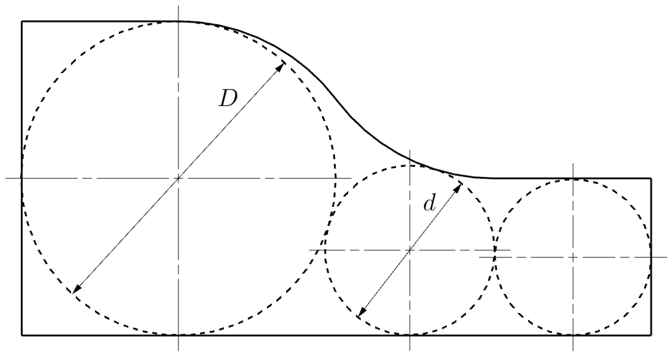
2.1.1. Heuvers’ Circles Method for Casting

Heuvers’ circles is a method to analyze cast parts for their manufacturability, first published in 1929 by Aloys Heuvers [23]. In casting, different cross-section sizes lead to different cooling and shrinking rates. The solidification of the material starts at the component’s surface while the material on the inside is still liquid. The solidified material can be compared to a shell, which cannot follow the shrinking rates of the inner material. Therefore, cavities can occur which cannot be filled by the liquid material anymore. To reduce the risk of cavities, the part has to be analyzed with the method of Heuvers’ circles.

To do so, circles are drawn into different cross-sections of the part (see Figure 1). The gradient of the diameters can be compared to a specific material factor. With this method, oversized cross-section changes can be detected and the risk of cavities can be reduced.

In general, the diameter ratio D/d of two contacting circles has to be lower than 1.6 [24]. For specific materials, lower diameter ratios have to be used. Typical Heuvers’ factors k_h are 1.0 to 1.5 [25].

An automated version of the Heuvers’ circles method has been proposed by Ransing et al. [15] to predict hot spots. They extend the method of Heuvers’ circles for three-dimensional geometries by using a medial axis transformation (3D-MAT). The MAT generates a medial axis for two-dimensional cross-sections (2D-MAT) or a medial surface for three-dimensional parts (3D-MAT), respectively, which are the centers of the generated Heuvers’ circles/spheres, and estimates their corresponding circle/sphere radii [15].

2.1.2. Evaluation Methods for Additive Manufacturing

In the realm of manufacturability analysis for additive manufacturing, several methods are proposed in the literature. First of all, the 3D-MAT as described before can be applied to analyze the geometry in a broader view not related to a specific manufacturing method [18,26].

Lambourne et al. propose an algorithm for computing the local thickness and the related medial surface representation [26]. To ensure accurate thickness estimation, a heuristic for surface sampling is provided: the element size s should be chosen to be smaller than the radius of 90% of the surface elements.

Bahlen et al. extend this approach by adding angle measurement to the computation of the 3D-MAT. Furthermore, they present a method for the classification of surface elements in wall and corner regions based on their corresponding position on the medial surface: The medial surface is separated into inner planes and stub planes, whereby stub planes are planes that touch the geometry’s surface while inner planes are only connected to other stub or inner planes. Surface elements that belong to stub planes are then considered to be corner regions, and all other elements are wall regions [18].

A conceptual method tailored to laser beam melting is proposed by Tominski et al. [19]. This method also applies the 3D-MAT to measure distances and angles. In addition, it incorporates overhang detection based on the comparison of neighboring surface normals and a routine to compute cross-sectional areas by slicing the geometry with cutting planes. Most notable is their proposition for feature classification: They propose to distinguish curvature and thickness measurement by the angle between the two normal vectors related to an inscribed sphere. However, they fail to define limit values for a proper distinction.

An alternative method to check for manufacturability with selective laser melting and sintering is demonstrated by Rudolph and Emmelmann [20]. Their method classifies surface elements into straight, convex, and concave environments by comparing the angles between neighboring normal vectors. Afterward, wall thicknesses and gap sizes are determined by measuring the distance of straight elements to the opposite elements, whereas convex and concave opposing pairs of elements are used to calculate cylinder and bore hole diameters, respectively. However, this method is restricted to the defined set of features and is not capable of evaluating edge sizes or free-form shapes.

Further methods for design evaluation are usage of the heat kernel signature, which recognizes features based on their heat transfer characteristics [27], a voxel-based representation [28], shape diameter functions [29], or machine learning approaches [30,31].

Moreover, an approach specifically tailored to WAAM using feature-based modeling and CAD macros is contributed by Lockett et al. [21]. Nevertheless, due to its dependence on feature-based modeling, this method restricts the design process to a specific CAD system and a limited set of features.

In addition, some works suggest the use of a database [19] or a manufacturability ontology [32,33] to relate manufacturability determining factors such as machinery, material, or process parameters to corresponding design constraints considered by the design evaluation tool. Thus, a comprehensive and flexible manufacturability evaluation system can be created, that supports manufacturability optimization in the design process by incorporating all relevant knowledge.

Lastly, it has to be noted that an alternative approach to foresee manufacturability in the design process is to conduct multiscale finite-element simulations of the whole process chain [17]. However, we focus in this work on pure geometric manufacturability analysis to provide immediate feedback to the designer. Nevertheless, customary FE simulations are not replaced, but rather complemented by geometric analysis based on design rules which could be fed by FE simulations. Thus, geometric analysis takes its place as the first element in the chain of computer-aided design tools, shortening the feedback loop by reflecting design constraints derived from the subsequent analysis steps.

2.2. Design Guidelines for WAAM

The assessment of designs is based on design rules. Traditionally, evaluation has been carried out by domain experts relying on their intuitive knowledge and experience [15], or is based on more systematic design guidelines, such as for casting [34] or as a reference for several fields [35]. In the field of design for additive manufacturing (DfAM), reviews of guidelines for several manufacturing technologies can be found [10,33]. Nevertheless, these guidelines are not applicable to WAAM, as Lockett et al. point out, since WAAM differs from other AM processes in its principal characteristics [3]. Therefore, specific guidelines for WAAM are needed.

The first design rules for WAAM based on experimental results and personal experience have been published in the works of Lockett et al. and Schmid [3,13] (see

Table 1. Design recommendations and constraints for WAAM manufactured components.

Feature	Recommendations and Constraints
general features	large, simple, sparsely detailed [13]
	limited number of bead ends [13]
	sudden cross-sectional changes avoided [13]
surface to volume ratio	high (for optimal heat transfer) [13]
symmetry or similar shapes	favor, to reduce warpage
	if applicable: base plate as symmetry plane [3,13]
part size	≥$50\mathrm{mm}$ (recommended for practical handling) [3]
	≤machine housing/enclosure (if applicable) [3]
min. wall thickness $w_{\min }$	$1.5\dots 2\mathrm{mm}$ (depends on process parameters) [3,13]
min. clearance	$0.9w_{\min }$ (for Al5A06) [36]
post-processing allowance	process dependent, e.g., machining $1\mathrm{mm}$ [37]
edges, corners	generously rounded [3]
	sharp corners either avoided or built as intersection [13]
overhangs	fixed torch: only angles ≥${45}^{°}$ possible [37]
	variable torch: arbitrary angles possible [38]
T-crossings	sharp, to avoid surface defects [13]
	alternative: optimized path planning strategies [39,40]
angles	simple path planning: ≥$58.{65}^{°}$ (for multi-bead walls) [41]
	optimized path planning: arbitrary angles [41],
	favor ≥${20}^{°}$ (for Al5A06) [36]

); however, several recommendations lack the quantitative criteria needed for automated design assessments.

More quantitative criteria can be found in studies concerning the manufacturing of specific features in specific problem settings (material, path planning strategy, tooling, etc.). In this regard, recommendations can be derived from studies on manufacturable overhang angles [37,38], constraints on corner angles, and path corrections to release these constraints [36,41], as well as investigations into T-crossings and possible path planning optimizations [39,40].

The most comprehensive compilation of WAAM-related design and manufacturing considerations can be found in the ASTM F3413 standard, which provides an overview of geometric features that can be manufactured using WAAM [42]. However, no quantitative criteria are stated for most features, except that the minimum wall thickness $w_{\min }$ is typically several millimeters. A summary of all recommendations is given in Table 1.

Overall, since WAAM is still in its childhood, design guidelines are merely general, imprecise, and subject to change by further research. Furthermore, the stated values heavily depend on the applied materials, path planning strategy, applied process parameters, and available machinery; therefore, they always have to be seen in the context of the specific manufacturing facilities.

3. Methods

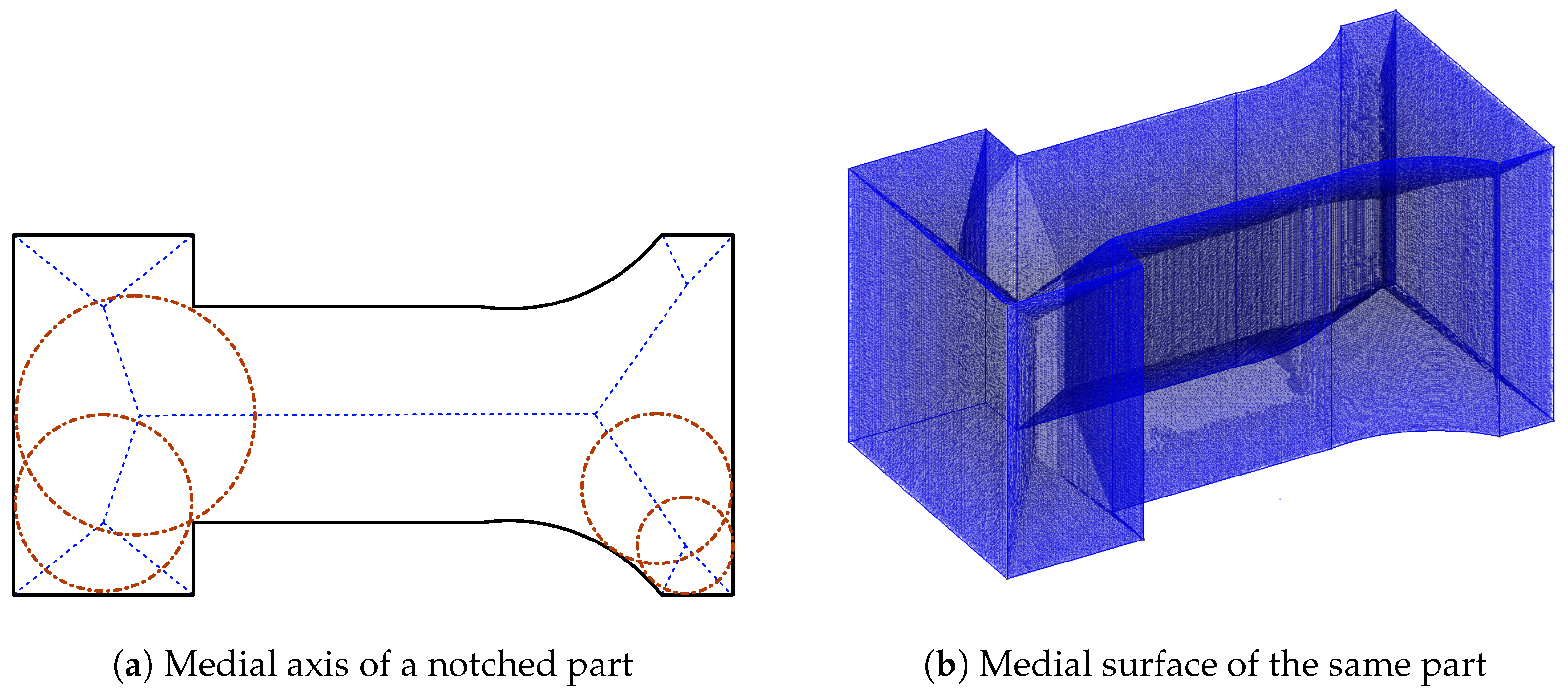
3.1. Medial Axis and Medial Surface Transformation

To assess the manufacturability of a geometry, it is necessary to define a set of indicators that describe the geometry features specified by the design rules for a specific manufacturing technology. In this study, the 3D-MAT method is applied and refined to assess the manufacturability with WAAM similar to Heuvers’ spheres method.

The medial axis transformation (MAT) is a transformation that returns a medial object, a dual representation of the input geometry. This dual representation is either a medial axis or a medial surface for 2D or 3D input geometries, respectively. It is defined as the set of all radii and midpoints of maximal circles/spheres inscribed in the geometry [43]. The medial object can thus be interpreted as the “skeleton” [43] or the local symmetry axis/plane of the transformed shape (see Figure 2a,b) while the associated radius correlates with the geometry’s local thickness. In our method for manufacturability assessment, we will use a medial surface representation of the input geometries; however, for ease of visualization, we illustrate the indicators on a medial axis.

The concept of Heuvers’ circles is related to the 3D-MAT in so far as the inscribed spheres and their radii are the three-dimensional counterparts of Heuvers’ circles and radii, respectively [15].

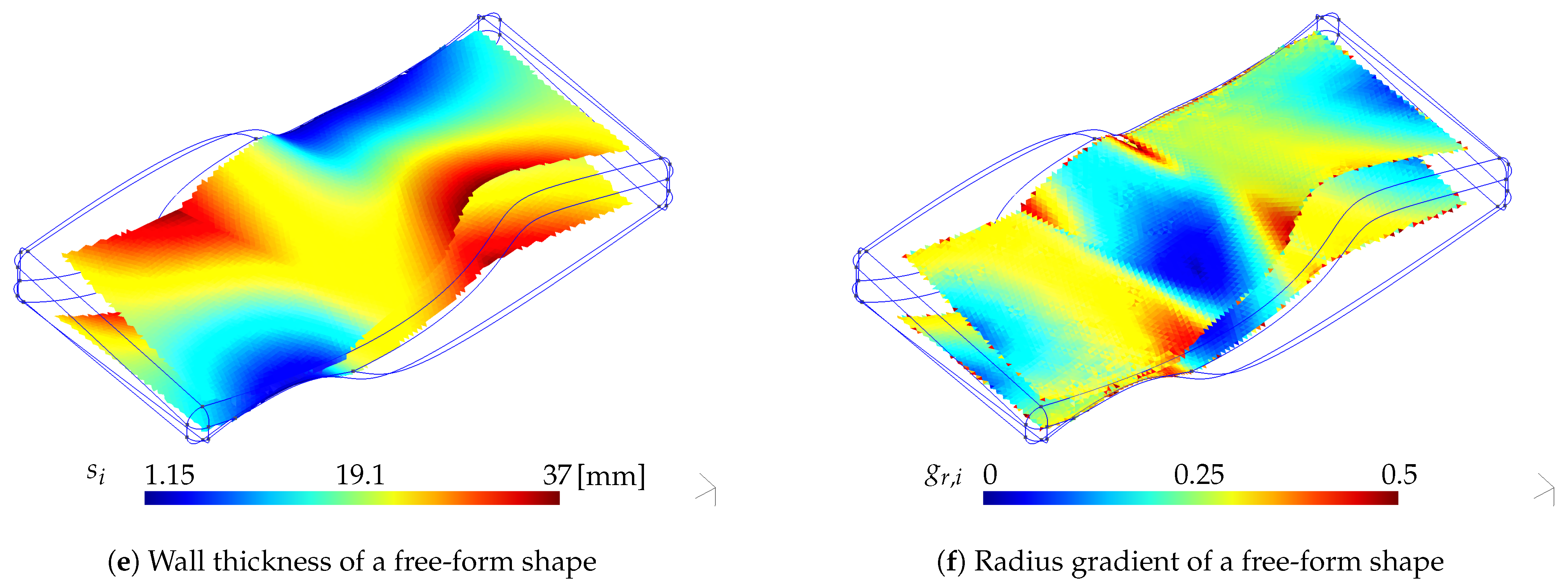
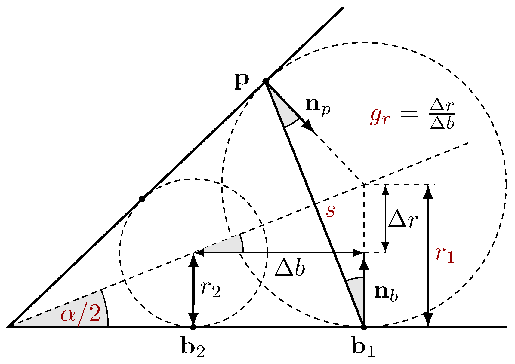
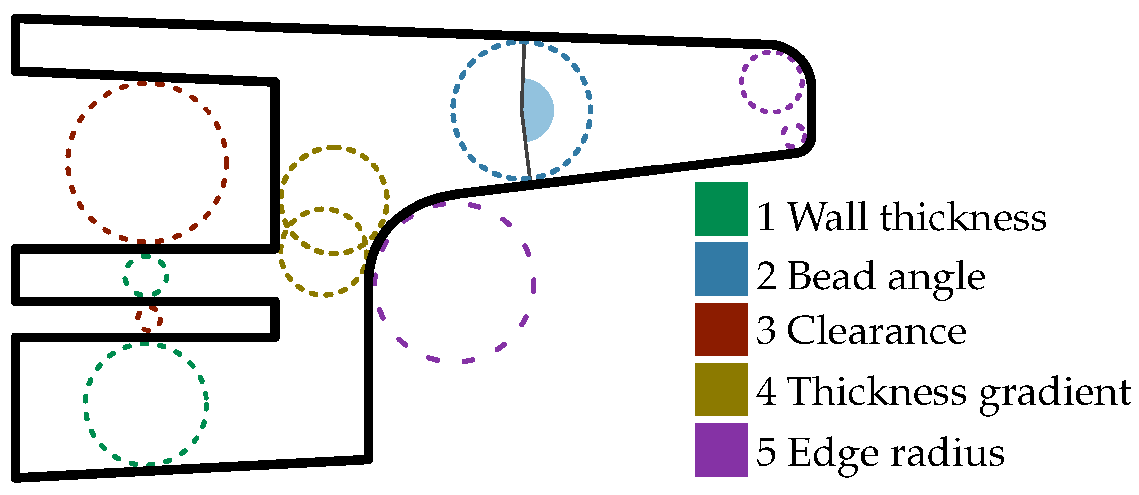
3.2. Definition of Geometry Indicators Based on the 3D-MAT

First of all, the radius derived from the 3D-MAT can be used to measure corner radii since two cases can occur: when moving on the medial surface into the corner, either the radius will go to zero for sharp edges or the corner’s curvature will coincide with the inscribed sphere.

For thickness measurement, however, the length of the secant $s=\parallel \mathbf{p}-\mathbf{b}\parallel$ between the two tangent points $\mathbf{p}$ and $\mathbf{b}$ of an inscribed sphere is more precise than the circle’s diameter, as Bahlen et al. point out [18], since the diameter would overestimate the thickness in relation to the angle enclosed by the surface normals (see Figure 3). Therefore, both indicators are used.

Additionally, the angle between the normal vector ${\mathbf{n}}_b$ to base point $\mathbf{b}$ and the secant length can be used to calculate the angle between two related faces according to Equation (1) (see Figure 3) [18].

$$\alpha =2arccos\left({\displaystyle \frac{(\mathbf{p}-\mathbf{b})·{\mathbf{n}}_b}{s}}\right)$$

(1)

Finally, the gradient of the radius function $g_r\left(\mathbf{x}\right)=\parallel \mathrm{grad}r\left(\mathbf{x}\right)\parallel$ can be defined as a fourth geometry indicator in correspondence to Heuvers’ ratios of neighboring circles. To compute the geometry indicators, the surface is discretized with a triangular mesh. Thus, every surface triangle of a watertight geometry has three adjacent triangles listed in the adjacency matrix $a(i,j)$: for a triangle with index i, the i-th row lists the three adjacent triangles in the columns $j=1\dots 3$. Consequently, the discrete gradient is obtained by Equation (2).

$$g_r\left(i\right)=\sqrt{\sum _{j=1}^3{\left({\displaystyle \frac{r\left(i\right)-r\left(a\right(i,j\left)\right)}{\parallel \mathbf{x}\left(i\right)-\mathbf{x}\left(a\right(i,j\left)\right)\parallel }}\right)}^2}$$

(2)

While a similar metric could be derived of the tangent of the half wall angle $tan{\displaystyle \frac{\alpha }{2}}$, which in fact is the gradient of the radius function in the direction of the medial axis, the formulation based on the radius function has the advantage of considering radius changes in all directions.

In summary, four indicators can be derived from the 3D-MAT to describe the geometry, which are the radius r, the secant length s, an angle $\alpha$, and the gradient of the radius function $g_r$. While Heuvers’ circles are usually inscribed in the geometry, the 3D-MAT can be calculated for the inside and the outside (inverse direction of surface normals) of the geometry, thus providing information about convex as well as concave parts. To differentiate the indicators derived from the inside 3D-MAT and the outside 3D-MAT, the indices ${(\_)}_i$ and ${(\_)}_o$, respectively, are used in the following.

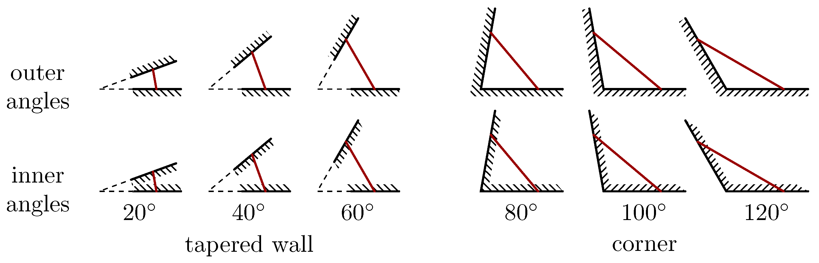
3.3. Application of WAAM Design Rules to 3D-MAT Geometry Indicators

The defined set of geometry indicators will be utilized to evaluate the manufacturing fitness of a part according to the design rules stated in Section 2.2. While the geometry indicators are computed over the complete geometry, the design rules usually apply only to certain features (like corners, walls, gaps, etc.) or regions (e.g., cross-sectional changes) of the geometry. Moreover, these features mentioned in manufacturability guidelines are often somewhat vague, and no exact geometric definitions of the features are stated. Therefore, a method has to be developed to classify elements of the discretized surface (that are triangles of the surface mesh) into regions that belong to a specified feature.

In the literature, two approaches to the classification of 3D-MAT results have been developed by Bahlen et al. [18] and Tominski et al. [19] (see Section 2.1.2). Whereas the method proposed by Bahlen et al. gives a clear distinction between wall and corner regions, the additional computation needed to segment the medial surface is rather complex. Therefore, we chose to expand the simpler method proposed by Tominski et al. to classify surface elements based on the angle information, thus reusing the geometry indicators. Consequently, for every assessed feature, a geometry indicator, a manufacturability constraint derived from the design guidelines, and a classification filter to restrict the design rule to the relevant region are needed.

The features considered by our approach are wall thickness, clearance, edge radius, bead angle, and thickness gradient (see Figure 4). In addition, the minimal and maximal part size could be checked by comparing the bounding box of the geometry to the specified limits. The other more general criteria, such as symmetry, surface-to-volume ratio, and overall complexity, are not considered by our approach. A summary of the considered design rules, their limit values, and their classification filters is given in

Table 2. Summary of considered design rules.

Feature	Indicator	Limits	Applied to Elements with …
wall thickness	$s_i$	≥$2\mathrm{mm}$	$0\le {\alpha }_i\le {65}^{°}$
clearance	$s_o$	≥$2\mathrm{mm}$	$0\le {\alpha }_o\le {65}^{°}$
edge radius	$r_i,r_o$	≥$5\mathrm{mm}$	${30}^{°}\le {\alpha }_i,{\alpha }_o\le {175}^{°}$
wall angle	${\alpha }_o$	≥${20}^{°}$	$s_o\le 5\mathrm{mm}$
thickness gradient	$g_{r,i}$	≤$0.23$	$0\le {\alpha }_i\le {65}^{°}$

.

The design guidelines for WAAM only specify a minimum wall thickness induced by machinery and process parameters. A part’s maximum thickness is until now not specified. Hence, a lower limit of $s\ge 2\mathrm{mm}$ is defined for wall thickness, measured by the secant’s length $s_i$ of the inside 3D-MAT. This rule is applied to opposing facets as classified by the wall angle.

There is a degree of freedom up to which angle a feature should be considered a thin tapered wall and from which angle it should be classified as a corner. Figure 5 shows various angles that can be classified as either a tapered wall or a corner. We set the limit to an angle of $0\le \alpha \le {65}^{°}$ for, in this region, the two facets can still reasonably be called facing each other, and experimental tests show a good differentiation of the two features with this choice. Nevertheless, the separation limit is only a matter of classification since thin elements would be detected as regions of a small corner radius if the limit was chosen differently.

Likewise, a lower limit of $s_{\mathrm{o}}\ge 2\mathrm{mm}$ is applied for clearance with the only difference that the secant length of the outside 3D-MAT is used. Classification is defined by the outer angle, analogously to the wall thickness. Note that the choice of $2\mathrm{mm}$ as the minimum limit is a conservative estimate since in the literature a value of $0.9w_{\min }$ (minimum wall thickness) is stated, albeit only for Al5A06 [36].

Towards the corner and edge radii, the literature gives no more quantitative recommendation than to choose them “generous” to allow for post-machining and to avoid stress raising [3]. Therefore, a lower limit of at least $r_{\mathrm{i},\mathrm{o}}\ge 5\mathrm{mm}$ is defined for acceptable radii in lack of more precise guidance. Since the guidelines specify no differences for convex and concave corners, the same constraint is defined for inner and outer radii. For the classification of corners, the same considerations hold as for the detection of walls except that the inverse region is now of interest. Nevertheless, we chose an overlapping region of ${30}^{°}\le \alpha \le {175}^{°}$ to have a conservative approach that highlights a non-manufacturable element twice rather than neglecting it.

Weld bead angles can be produced in arbitrary angles if path planning corrections are employed; however, $\alpha \ge {20}^{°}$ should be favored to avoid distortion [36], which is why we implement this recommendation on outer angles. The mentioned design rule relates to angle-induced distortion between distinct walls; therefore, the outer angle information is used. Since this distortion occurs only in weld bead’s vertices, the restriction is limited to regions of small outer distance. We chose secant lengths of $s_{\mathrm{o}}\le 5\mathrm{mm}$ as a limit for these regions.

Finally, the gradient indicator is used to spot regions of mass accumulation or sudden cross-sectional changes such as T-crossings which affect the heat transfer rate and in consequence warpage. At the current state of research, there are no quantitative recommendations for allowed gradients defined yet. Since the heat transfer problem in WAAM is similar to casting, the analogy of the Heuvers’ spheres to the 3D-MAT is exploited to estimate maximal allowable gradients by the corresponding Heuvers’ factors. Heuvers’ factors limit the diameter ratio of touching inscribed circles. This factor $k_{\mathrm{H}}={\displaystyle \frac{r_2}{r_1}}$ can be transformed to a thickness gradient according to Equation (3):

$$g_{\mathrm{r}}={\displaystyle \frac{r_2-r_1}{r_1+r_2}}={\displaystyle \frac{k_{\mathrm{H}}-1}{k_{\mathrm{H}}+1}}.$$

(3)

For a typical Heuvers’ factor of $k_{\mathrm{H}}=1.6$, the maximum limit of the thickness gradient is consequently $g_{\mathrm{r}}=0.23$. This constraint is applied to wall elements as classified for the thickness measurement since corners are not regions of high mass accumulation despite high radius gradients.

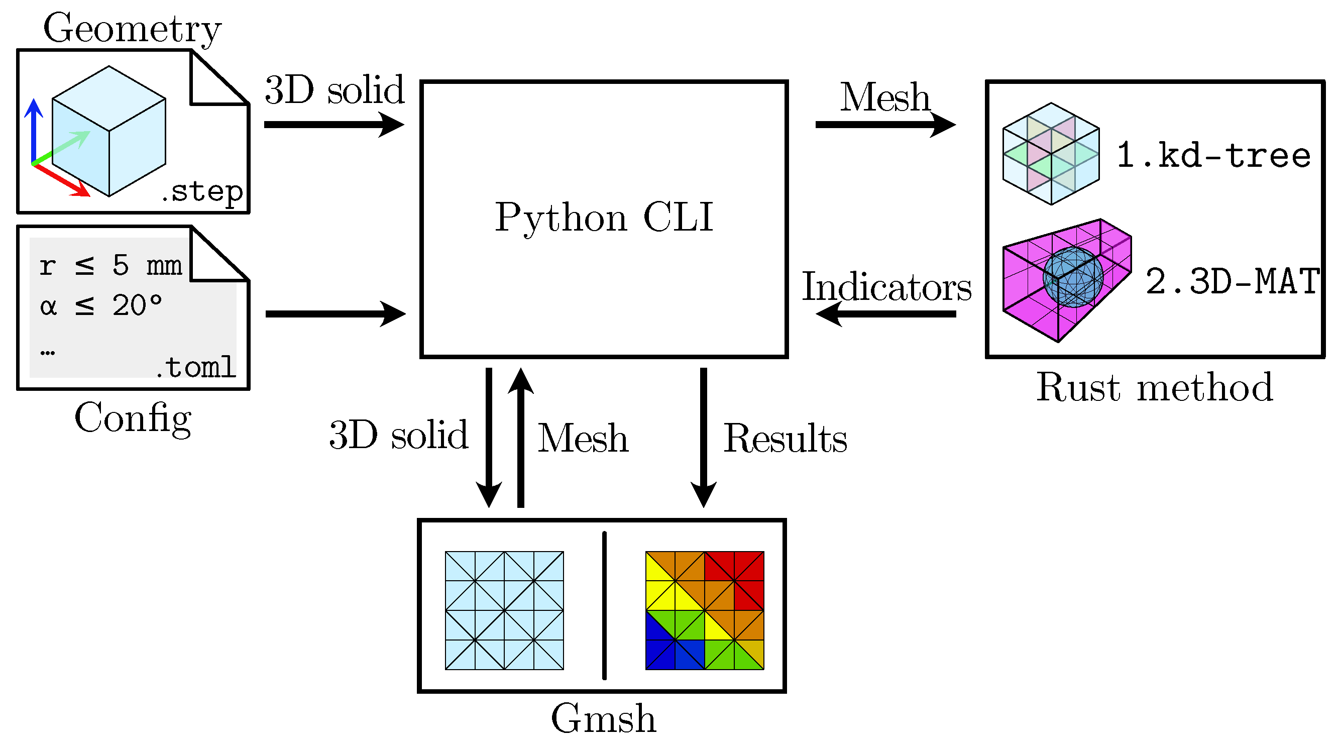
3.4. Test Implementation

In order to test the proposed method, we have written a command line software, which takes Step files as input and highlights critical facets in Gmsh (Gmsh is “a three-dimensional finite element mesh generator with built-in pre- and post-processing facilities” [44]). For performance reasons, a combined Python–Rust (Rust is a modern system-level programming language like C++ that allows performant execution while ensuring memory safety [45]) architecture was chosen of which Figure 6 gives an overview. The source code and the tested example parts are available through a GitLab repository [46].

To facilitate simple adaption of design constraints and feature classification to varied manufacturing capabilities, a flexible configuration file based on the Toml (Toml is a simple human-readable configuration format based on text files [47]) format was developed. The configuration file allows the definition of design features with their corresponding design constraints and classification filters. The classification filters restrict the application of the design constraints to a certain geometry region.

The evaluation of a geometry can roughly be divided into the three stages: pre-, main-, and post-processing. In detail, the steps are as follows:

• Via Python, Gmsh is controlled to load the 3D solid geometry in the Step format. Gmsh then triangulates the surface according to a specified element size.
• The generated mesh data, which are the triangles’ center points and face normals, are then handed over to a Rust method. In the Rust method, first, a kd-tree is built from the point data, and then the 3D-MAT is calculated using the shrinking ball algorithm [48].
  A kd-tree is a space-partitioning method that enables efficient nearest neighbor search on point clouds, which improves the computational performance of the 3D-MAT algorithm. The kd-tree is a binary search tree that is built by alternatingly dividing the geometry along the three spatial axes into subspaces until in every subspace only a defined number of points is left [49].
  The shrinking ball algorithm developed by Ma et al. approximates the 3D-MAT for every surface point and the corresponding surface normal by iteratively shrinking spheres to fit them into the 3D point cloud. Starting with the initial radius set to the maximum diameter of the axis-aligned bounding box, the current sphere center is calculated:

  $$\mathbf{c}=\mathbf{b}+r^i{\mathbf{n}}_b.$$

  (4)
  An updated radius $r^{i+1}$ is then derived according to Equations (5) and (6) with $\mathbf{p}$ being the nearest neighbor to $\mathbf{c}$ that is within the radius $r^i$ and is different from the base point $\mathbf{b}$ (cmp. Figure 3) [50]. The nearest neighbor is efficiently found by performing the search on the kd-tree. This iteration is repeated until no point is found that satisfies the criteria, indicating an empty sphere.

  $$\begin{array}{cc}\hfill s& =\parallel \mathbf{p}-\mathbf{b}\parallel \hfill \end{array}$$

  (5)

  $$\begin{array}{cc}\hfill r^{i+1}& ={\displaystyle \frac{s}{2}}(\mathbf{p}-\mathbf{b})·\mathbf{n}\hfill \end{array}$$

  (6)
  Finally, the angle $\alpha$ is calculated using Equation (1), and the calculated radii, distances (secant lengths), and angles are returned to the Python program.
• In the Python program, the radii gradients are calculated over neighboring facets (Equation (2)). Then, for every feature, the particular indicator data are filtered by another indicator as specified in the configuration file. To visualize the results, the filtered data are feature-wise added to Gmsh, whereby the highlighted faces are restricted to those critical according to the specified manufacturing limits.

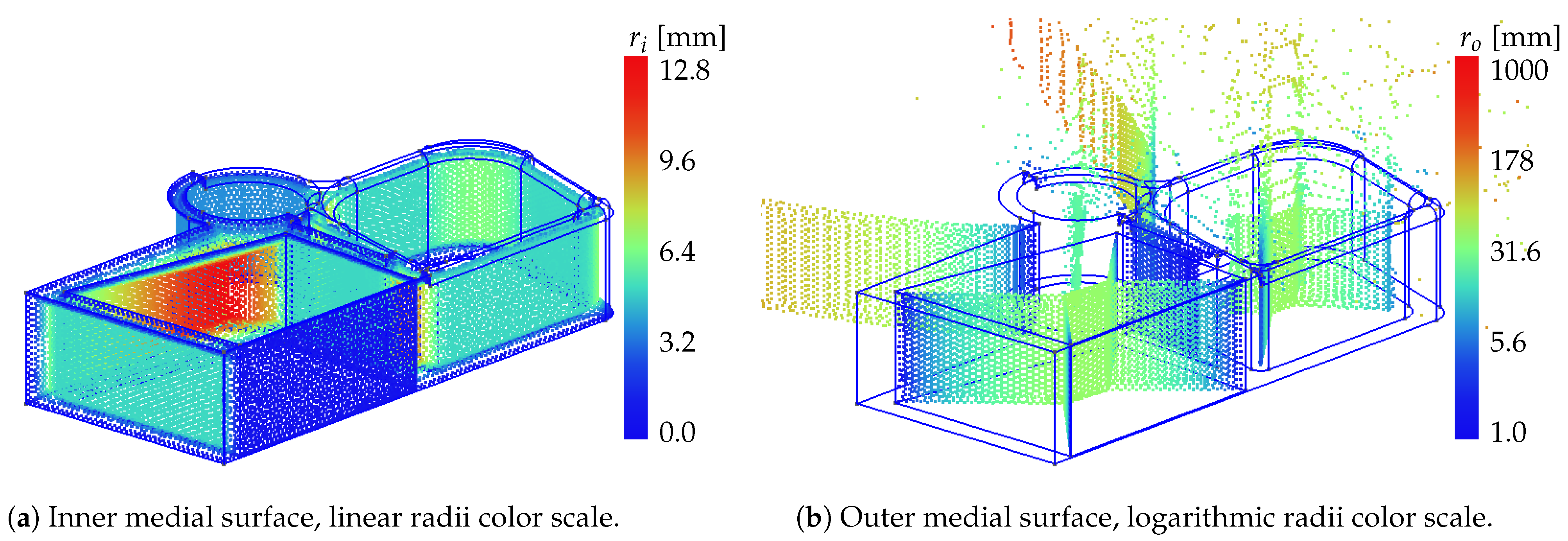
4. Results on Example Geometries

We used an example bar part with several design flaws (left-hand side) and corresponding corrections (right-hand side) to demonstrate and verify our implementation (see Figure 7). The smallest wall thickness measures $1\mathrm{mm}$ (not manufacturable) while the largest wall thickness is around $29\mathrm{mm}$, and leads to a mass accumulation. The part exhibits 13 concave and 13 convex edges, rounded with a radius of at least $5\mathrm{mm}$ on the right-hand side and, conversely, sharp-edged on the left-hand side. In the center, a tapered slot was introduced with an angle of ${11}^{°}$ and a maximum opening of $10\mathrm{mm}$ to test the detection of small angles and small clearances.

The implementation classifies most elements properly and reveals all intended design errors in our example. However, our implementation of the shrinking ball algorithm reports minor convergence issues. In our test example for 99 out of 50,014 points (≈$2.0$‰), the iteration aborted by reaching the maximum number of iterations instead of meeting the empty sphere criteria. Nonetheless, for most of these elements, the results were still valid, since the last iterations all yielded the same values.

The resulting approximated medial surfaces for the inner and outer 3D-MAT, respectively, are presented in Figure 8a,b. The center points are color-coded from blue to red for small to large radii. While the results look mostly as expected like a local symmetry plane of the geometry, the right-hand side of the outer medial surface shows loosely spread center points around the rounded edges. This originates from the surface discretization: on a perfectly round continuous surface, every tangent sphere would have an infinite radius and thus the center point would be infinitely far away from the surface (as is the case for the plane surfaces). However, through the surface discretization, the triangle’s normal vectors are deviated and the tangential spheres intersect with adjacent triangles, resulting in non-infinite sphere radii.

Figure 9a–f show the results of the manufacturability evaluation; critical elements are highlighted in their severity from yellow to red.

The wall thickness and clearance rule properly detect the corresponding design flaws and do not highlight any false positives. Only the thin wall element does not appear as a plane face but is spotted, which relates to irregular angle results in that region, which are used as a classification filter.

The edge rules generally show the same results as the thickness and clearance rules. However, the critically thin wall is classified as edge, which is caused by the same angle-related issue as reported above. On interpreting the results, it has to be noted that the upper left rounding radius has the same value as the radius limit; therefore, they would be manufacturable. Furthermore, the bottom layer edges would be manufacturable too, despite being highlighted properly according to the defined rule. Since in the WAAM process a part is built up on a base plate, it is possible to manufacture sharp edges on the base layer. Nevertheless, since our implementation has no information on the part’s build orientation, this detail cannot be considered.

The low angle between the middle bars and the radius gradients is detected as well. However, while the angle shows clear results, the gradient classification shows issues. The thin wall is again falsely included, and some elements were not filtered out in the transitions from corner to wall.

In addition to the example geometry presented here, we tested our method on several benchmark geometries regarding the wall thickness, the edge radii, the radius gradient, and the wall angle yielding similar results (see Figure A1a–f in Appendix A).

5. Discussion

The computational performance of our approach is mainly governed by the four main computing stages which are (1) building the kd-tree, (2) computation of the 3D-MAT, (3) computation of the gradient, and (4) filtering the computed data. Since the actual computation time directly depends on the computation hardware and implementation-specific details (such as programming language-specific optimizations), an algorithm’s performance is best compared by its computational complexity usually denoted in $\mathcal{O}$-notation. The effort to build the kd-tree is bound to $\mathcal{O}(nlogn)$ and nearest neighbor searching can be performed with $\mathcal{O}(logn)$ [51]. Thus, the computation of the 3D-MAT for n-elements can be described by $\mathcal{O}(2nlogn)$ taking into account that the 3D-MAT has to be calculated for the in- and outside. However, the computation of the adjacency matrix, needed for the gradient calculation, is in the simplest form of the order $\mathcal{O}\left(n^2\right)$, since for every triangle n a search over all n triangles has to be performed to find the adjacent ones. Finally, the filtering can be performed with $\mathcal{O}\left(fn\right)$, since the filter criteria have to be checked once per feature f for every element. Overall, the complexity of our approach can therefore be estimated to be of the order

$$\mathcal{O}(nlogn)+\mathcal{O}(2nlogn)+\mathcal{O}\left(n^2\right)+\mathcal{O}\left(fn\right)=\mathcal{O}\left(n^2\right).$$

(7)

Note that $\mathcal{O}\left(n^2\right)$ is the complexity of the matrix vector multiplication of an $n\times n$ matrix. While estimations of the computational complexity of finite element methods depend on the specific problem and the applied solution strategy, finite element methods have to solve at least a matrix vector multiplication of a vector holding n boundary conditions for the surface elements with an $m\times n$ matrix for a body with m elements in total ($m\ge n$), which yields to an estimated complexity of at least $\mathcal{O}\left(mn\right)$. Therefore, we expect our method to perform at least comparably to finite element methods in terms of computation complexity.

Furthermore, our approach can even be expected to perform better than finite element analysis of the process chain when considering that only a static analysis of the surface is needed instead of solving a time integration problem of the whole manufacturing process.

In addition to the test example presented in Section 4, further tests on benchmark parts have been conducted which showed similar results. Furthermore, we expect our approach to produce valid results on virtually any arbitrary geometry that permits inscribing spheres as long as an acceptable mesh quality can be achieved, since the presented method assesses manufacturability only on local geometry characteristics.

Overall, our implementation is capable of automatically checking the stated design rules for medium-complex parts. However, issues in convergence and classification can occur as stated in Section 4.

The false classification of the thin wall traces back to erroneous angle estimation in that region. Due to the relatively rough surface discretization compared to the wall thickness, corresponding triangle center points (which are the base points for the calculation of the 3D-MAT) do not coincide. This deviation leads to an overestimation of the angle enclosed between the surface normal and the secant connecting the two corresponding points (compare Figure 3). This finding is further bolstered when considering the sensitivity of the angle computation to deviations of the secant length: the sensitivity

$${\displaystyle \frac{\partial }{\partial s}}\arccos \left({\displaystyle \frac{(\mathbf{p}-\mathbf{b})·{\mathbf{n}}_b}{s}}\right)={\displaystyle \frac{1}{\sqrt{{\left(\frac{s}{(\mathbf{p}-\mathbf{b})·{\mathbf{n}}_b}\right)}^2-1}}}$$

(8)

goes to infinity for s approaching $(\mathbf{p}-\mathbf{b})·{\mathbf{n}}_b$, which happens for parallel elements. That means small deviations of s will lead to large deviations of $\alpha$ for parallel elements. In fact, tests with a smaller element size (and thus smaller deviation) produced better angle estimations, albeit still in an unacceptable region compared to the needed computational effort. However, this problem could be circumvented by reformulating the angle equation to derive the angle by using the dot product of both normal vectors, thus avoiding the secant length. In addition, adaptive meshing methods could be used to automatically adapt the mesh size to small features.

In order to improve the 3D-MAT convergence, the termination condition could be improved by respecting both the empty sphere criteria and the analysis of the radius change over several iterations. Additionally, the effect of the surface discretization can be lowered based on an approach avoiding sphere intersections with nearby elements [52].

Furthermore, the concept could be extended to consider a part’s build orientation to allow the evaluation of overhang angles or layer-specific rules, such as sharp edges on the base plate, which would require the usage of more complex classification filters (e.g., the Boolean junction of two filters). Finally, experimental validation of the fitness evaluation results is needed, as well as further research to refine the quantification and applicability of design constraints. In particular, the gradient limit estimated by Heuvers’ factor should be investigated by considering the heat transfer problem.

6. Conclusions

An approach to fitness evaluation for manufacturing with WAAM based on geometric reasoning was shown, which allows, in contrast to time-consuming finite element analysis, for immediate feedback in the design process. The key contributions of our work are as follows:

• The mapping of current WAAM design recommendations to corresponding MAT geometry indicators.
• The definition of quantitative criteria for feature classification in 3D-MAT-based manufacturability evaluation.
• The addition of the radius gradient to the set of MAT geometry indicators.

To test the effectiveness of our method in finding violations of WAAM design rules from the literature, we ran a test implementation on a set of feature benchmarks (see Figure A1a–f in Appendix A) and discussed the results for an example part. While all design rule violations were recognized in the example, some limitations regarding noise, feature classification of thin wall sections, and the calculation of the gradient were found. However, directions for further improvements to relieve these issues were shown. Nevertheless, further research is also needed to refine existing design recommendations for WAAM and to prove the effectiveness of our method with experimental results.

With our method of automated manufacturability analysis, we provide designers with a tool that gives easy access to the latest technology improvements while shortening the analysis time through geometric reasoning. The flexible definition of design and classification rules allows the current state of technology to be steadily reflected to the industrial designer.

References

1. Ding, D.; Pan, Z.; Cuiuri, D.; Li, H. Wire-Feed Additive Manufacturing of Metal Components: Technologies, Developments and Future Interests. Int. J. Adv. Manuf. Technol. 2015, 81, 465–481. [Google Scholar] [CrossRef]
2. Roy, S.; Shassere, B.; Yoder, J.; Nycz, A.; Noakes, M.; Narayanan, B.K.; Meyer, L.; Paul, J.; Sridharan, N. Mitigating Scatter in Mechanical Properties in AISI 410 Fabricated via Arc-Based Additive Manufacturing Process. Materials 2020, 13, 4855. [Google Scholar] [CrossRef] [PubMed]
3. Lockett, H.; Ding, J.; Williams, S.; Martina, F. Design for Wire + Arc Additive Manufacture: Design Rules and Build Orientation Selection. J. Eng. Des. 2017, 28, 568–598. [Google Scholar] [CrossRef]
4. Treutler, K.; Wesling, V. The Current State of Research of Wire Arc Additive Manufacturing (WAAM): A Review. Appl. Sci. 2021, 11, 8619. [Google Scholar] [CrossRef]
5. Huang, L.; Chen, X.; Konovalov, S.; Su, C.; Fan, P.; Wang, Y.; Xiaoming, P.; Panchenko, I. A Review of Challenges for Wire and Arc Additive Manufacturing (WAAM). Trans. Indian Inst. Met. 2023, 76, 1123–1139. [Google Scholar] [CrossRef]
6. Chaturvedi, M.; Scutelnicu, E.; Rusu, C.C.; Mistodie, L.R.; Mihailescu, D.; Subbiah, A.V. Wire Arc Additive Manufacturing: Review on Recent Findings and Challenges in Industrial Applications and Materials Characterization. Metals 2021, 11, 939. [Google Scholar] [CrossRef]
7. Rodrigues, T.A.; Duarte, V.; Miranda, R.; Santos, T.G.; Oliveira, J. Current Status and Perspectives on Wire and Arc Additive Manufacturing (WAAM). Materials 2019, 12, 1121. [Google Scholar] [CrossRef] [PubMed]
8. Williams, S.W.; Martina, F.; Addison, A.C.; Ding, J.; Pardal, G.; Colegrove, P. Wire + Arc Additive Manufacturing. Mater. Sci. Technol. 2016, 32, 641–647. [Google Scholar] [CrossRef]
9. Evans, S.I.; Wang, J.; Qin, J.; He, Y.; Shepherd, P.; Ding, J. A review of WAAM for steel construction—Manufacturing, material and geometric properties, design, and future directions. Structures 2022, 44, 1506–1522. [Google Scholar] [CrossRef]
10. Thompson, M.K.; Moroni, G.; Vaneker, T.; Fadel, G.; Campbell, R.I.; Gibson, I.; Bernard, A.; Schulz, J.; Graf, P.; Ahuja, B.; et al. Design for Additive Manufacturing: Trends, Opportunities, Considerations, and Constraints. CIRP Ann. 2016, 65, 737–760. [Google Scholar] [CrossRef]
11. Mehnen, J.; Ding, J.; Lockett, H.; Kazanas, P. Design for Wire and Arc Additive Layer Manufacture. In Global Product Development; Bernard, A., Ed.; Springer: Berlin/Heidelberg, Germany, 2011; pp. 721–727. [Google Scholar] [CrossRef]
12. Wei, H.L.; Bhadeshia, H.K.D.H.; David, S.A.; DebRoy, T. Harnessing the scientific synergy of welding and additive manufacturing. Sci. Technol. Weld. Join. 2019, 24, 361–366. [Google Scholar] [CrossRef]
13. Schmid, C. Konstruktive Randbedingungen bei Anwendung des WAAM-Verfahrens. In Konstruktion für die Additive Fertigung 2019; Lachmayer, R., Rettschlag, K., Kaierle, S., Eds.; Springer: Berlin/Heidelberg, Germany, 2020; pp. 203–222. [Google Scholar] [CrossRef]
14. Greer, C.; Nycz, A.; Noakes, M.; Richardson, B.; Post, B.; Kurfess, T.; Love, L. Introduction to the design rules for Metal Big Area Additive Manufacturing. Addit. Manuf. 2019, 27, 159–166. [Google Scholar] [CrossRef]
15. Ransing, R.; Sood, M.; Pao, W. Computer Implementation of Heuvers’ Circle Method for Thermal Optimisation in Castings. Int. J. Cast Met. Res. 2005, 18, 119–128. [Google Scholar] [CrossRef]
16. Mehnen, J.; Ding, J.; Lockett, H.; Kazanas, P. Design Study for Wire and Arc Additive Manufacture. Int. J. Prod. Dev. 2014, 19, 2. [Google Scholar] [CrossRef]
17. Besong, L.I.B.; Buhl, J. A Review of Constitutive Models Used in Macroscale Finite Element Analysis of Additive Manufacturing and Post-Processing of Additively Manufactured Components. Virtual Phys. Prototyp. 2024, 19, e2356079. [Google Scholar] [CrossRef]
18. Bahlen, T.M.; Bronsvoort, W.F.; Spence, A.D. Extraction and Visualization of Dimensions from a Geometric Model. Comput.-Aided Des. Appl. 2010, 7, 579–589. [Google Scholar] [CrossRef]
19. Tominski, J.; Lammers, S.; Wulf, C.; Zimmer, D. Method for a Software-Based Design Check of Additively Manufactured Components. In Proceedings of the 29th Annual International Solid Freeform Fabrication Symposium–An Additive Manufacturing Conference, Austin, TX, USA, 13–15 August 2018; pp. 69–79. [Google Scholar] [CrossRef]
20. Rudolph, J.P.; Emmelmann, C. Analysis of Design Guidelines for Automated Order Acceptance in Additive Manufacturing. Procedia CIRP 2017, 60, 187–192. [Google Scholar] [CrossRef]
21. Lockett, H.; Emms, R.; Williams, S.; Ding, J.; Martina, F. The Application of Knowledge Based Engineering to Design for Wire+Arc Additive Manufacture (WAAM). In Proceedings of the 6th Aircraft Structural Design Conference, Bristol, UK, 9–11 October 2018. [Google Scholar]
22. Ye, J.; Kyvelou, P.; Gilardi, F.; Lu, H.; Gilbert, M.; Gardner, L. An End-to-End Framework for the Additive Manufacture of Optimized Tubular Structures. IEEE Access 2021, 9, 165476–165489. [Google Scholar] [CrossRef]
23. Heuvers, A. Was hat der Stahlgießer dem Konstrukteur über Lunker- und Rißbildung zu sagen? Stahl Und Eisen 1929, 49, 1239–1256. [Google Scholar]
24. Geupel, H. Konstruktionslehre; Springer: Berlin/Heidelberg, Germany, 1996. [Google Scholar]
25. Fritz, A.H. (Ed.) Fertigungstechnik; Springer: Berlin/Heidelberg, Germany, 2018. [Google Scholar] [CrossRef]
26. Lambourne, J.; Djuric, Z.; Brujic, D.; Ristic, M. Calculation and visualisation of the thickness of 3D CAD models. In Proceedings of the International Conference on Shape Modeling and Applications 2005, Cambridge, MA, USA, 13–17 June 2005; pp. 338–342. [Google Scholar] [CrossRef]
27. Shi, Y.; Zhang, Y.; Baek, S.; De Backer, W.; Harik, R. Manufacturability Analysis for Additive Manufacturing Using a Novel Feature Recognition Technique. Comput.-Aided Des. Appl. 2018, 15, 941–952. [Google Scholar] [CrossRef]
28. Tedia, S.; Williams, C.B. Manufacturability Analysis Tool for Additive Manufacturing Using Voxel-Based Geometric Modeling. In Proceedings of the 27th Annual International Solid Freeform Fabrication Symposium 2016—An Additive Manufacturing Conference, Austin, TX, USA, 8–10 August 2016; pp. 3–22. [Google Scholar]
29. Jaiswal, P.; Rai, R. A Geometric Reasoning Approach for Additive Manufacturing Print Quality Assessment and Automated Model Correction. Comput.-Aided Des. 2019, 109, 1–11. [Google Scholar] [CrossRef]
30. Sunil, V.B.; Pande, S.S. Automatic Recognition of Machining Features Using Artificial Neural Networks. Int. J. Adv. Manuf. Technol. 2009, 41, 932–947. [Google Scholar] [CrossRef]
31. Mycroft, W.; Katzman, M.; Tammas-Williams, S.; Hernandez-Nava, E.; Panoutsos, G.; Todd, I.; Kadirkamanathan, V. A data-driven approach for predicting printability in metal additive manufacturing processes. J. Intell. Manuf. 2020, 31, 1769–1781. [Google Scholar] [CrossRef]
32. Han, J.; Schaefer, D. An Ontology for Supporting Digital Manufacturability Analysis. Procedia CIRP 2019, 81, 850–855. [Google Scholar] [CrossRef]
33. Mayerhofer, M.; Lepuschitz, W.; Hoebert, T.; Merdan, M.; Schwentenwein, M.; Strasser, T.I. Knowledge-Driven Manufacturability Analysis for Additive Manufacturing. IEEE Open J. Ind. Electron. Soc. 2021, 2, 207–223. [Google Scholar] [CrossRef]
34. Campbell, J. Chapter 10—The 10 Rules for Good Castings. In Complete Casting Handbook; Butterworth-Heinemann: Oxford, UK, 2011; pp. 605–737. [Google Scholar] [CrossRef]
35. Bralla, J.G. (Ed.) Design for Manufacturability Handbook, 2nd ed.; McGraw-Hill Handbooks; McGraw-Hill: Boston, MA, USA, 1999. [Google Scholar]
36. Geng, H.; Li, J.; Xiong, J.; Lin, X.; Zhang, F. Geometric Limitation and Tensile Properties of Wire and Arc Additive Manufacturing 5A06 Aluminum Alloy Parts. J. Mater. Eng. Perform. 2017, 26, 621–629. [Google Scholar] [CrossRef]
37. Song, Y.A.; Park, S.; Choi, D.; Jee, H. 3D Welding and Milling: Part I–a Direct Approach for Freeform Fabrication of Metallic Prototypes. Int. J. Mach. Tools Manuf. 2005, 45, 1057–1062. [Google Scholar] [CrossRef]
38. Kazanas, P.; Deherkar, P.; Almeida, P.; Lockett, H.; Williams, S. Fabrication of Geometrical Features Using Wire and Arc Additive Manufacture. Proc. Inst. Mech. Eng. Part B J. Eng. Manuf. 2021, 226, 1042–1051. [Google Scholar] [CrossRef]
39. Venturini, G.; Montevecchi, F.; Scippa, A.; Campatelli, G. Optimization of WAAM Deposition Patterns for T-crossing Features. Procedia CIRP 2016, 55, 95–100. [Google Scholar] [CrossRef]
40. Li, R.; Zhang, H.; Dai, F.; Huang, C.; Wang, G. End lateral extension path strategy for intersection in wire and arc additive manufactured 2319 aluminum alloy. Rapid Prototyp. J. 2019, 26, 360–369. [Google Scholar] [CrossRef]
41. Liu, H.H.; Zhao, T.; Li, L.Y.; Liu, W.J.; Wang, T.Q.; Yue, J.F. A Path Planning and Sharp Corner Correction Strategy for Wire and Arc Additive Manufacturing of Solid Components with Polygonal Cross-Sections. Int. J. Adv. Manuf. Technol. 2020, 106, 4879–4889. [Google Scholar] [CrossRef]
42. ASTM F3413-19e1; Guide for Additive Manufacturing—Design–Directed Energy Deposition. ASTM International: West Conshohocken, PA, USA, 2020. [CrossRef]
43. Blum, H. A Transformation for Extracting New Descriptors of Shape. In Models for Perception of Speech and Visual Form; Wathen-Dunn, W., Ed.; MIT Press: Cambridge, MA, USA, 1967; pp. 362–380. [Google Scholar]
44. Geuzaine, C.; Remacle, J.F. Gmsh: A 3-D Finite Element Mesh Generator with Built-in Pre- and Post-Processing Facilities: THE GMSH PAPER. Int. J. Numer. Methods Eng. 2009, 79, 1309–1331. [Google Scholar] [CrossRef]
45. Matsakis, N.D.; Klock, F.S., II. The rust language. ACM SIGAda Ada Lett. 2014, 34, 103–104. [Google Scholar] [CrossRef]
46. Stromberg, H.; Pusicha, J. WAAM_fit GitLab Repository. Available online: https://gitlab.tu-clausthal.de/jpu18/WAAM_fit (accessed on 5 February 2024).
47. Preston-Werner, T.; Gedam, P. TOML v1.0.0. Available online: https://toml.io/en/v1.0.0 (accessed on 25 May 2024).
48. Ma, J.; Bae, S.W.; Choi, S. 3D Medial Axis Point Approximation Using Nearest Neighbors and the Normal Field. Vis. Comput. 2011, 28, 7–19. [Google Scholar] [CrossRef]
49. Bentley, J.L. Multidimensional Binary Search Trees Used for Associative Searching. Commun. ACM 1975, 18, 509–517. [Google Scholar] [CrossRef]
50. Bayardo Spadafora, J.; Gomez-Fernandez, F.; Taubin, G. Fast Non-Convex Hull Computation. In Proceedings of the 2019 International Conference on 3D Vision (3DV), Québec City, QC, Canada, 16–19 September 2019; pp. 747–755. [Google Scholar] [CrossRef]
51. Friedman, J.H.; Bentley, J.L.; Finkel, R.A. An Algorithm for Finding Best Matches in Logarithmic Expected Time. ACM Trans. Math. Softw. 1977, 3, 209–226. [Google Scholar] [CrossRef]
52. Peters, R. Geographical point cloud modelling with the 3D medial axis transform. Ph.D. Thesis, Delft University of Technology, Delft, The Netherlands, 2018. [Google Scholar] [CrossRef]
Figure 1. Example for Heuvers’ circles with different diameters D and d.
Applsci 15 00938 g001
Figure 2. Medial axis and medial surface as dual representation of a geometry delivering its local symmetry axis or plane. The medial axis and the medial surface are defined by the set of all midpoints of maximally inscribed circles and spheres, respectively.
Applsci 15 00938 g002
Figure 3. Dimensions of the 3D-MAT: p , b : tangent points; n p , n b : normal vectors; α : wall angle; s: secant; g r : 2D gradient.
Applsci 15 00938 g003
Figure 4. Different applications of Heuvers’ sphere.
Applsci 15 00938 g004
Figure 5. Comparison of various outer and inner angles and the secant used (red). Sections with an enclosed angle of 0 α 65 ° can be considered as tapered wall.
Applsci 15 00938 g005
Figure 6. Overview of the implemented software architecture.
Applsci 15 00938 g006
Figure 7. Example bar part to verify our implementation. Design flaws on the left-hand side, and corresponding corrections on the right-hand side. All dimensions are indicated in millimeters.
Applsci 15 00938 g007
Figure 8. Approximations of the medial surfaces of the example part. The center points of the inscribed spheres are color-coded by their radius in millimeters.
Applsci 15 00938 g008
Figure 9. Evaluation results on the example part. For each feature, non-manufacturable faces are highlighted with a color scale from yellow to red with ascending constraint violation.
Applsci 15 00938 g009