Article

Short-Term Photovoltaic Output Prediction Method Based on Data Decomposition and Error Correction

1
State Key Laboratory of Power Transmission Equipment Technology, School of Electrical Engineering, Chongqing University, Chongqing 400044, China
2
State Grid Gansun Electric Power Research Institute, Lanzhou 730070, China
*
Author to whom correspondence should be addressed.
Appl. Sci. 2025, 15(20), 11089; https://doi.org/10.3390/app152011089
Submission received: 29 August 2025 / Revised: 8 October 2025 / Accepted: 13 October 2025 / Published: 16 October 2025

Abstract

Considering the limited availability of meteorological data in practice, this paper investigates the short-term photovoltaic output prediction problem based on data decomposition and error correction to further improve prediction accuracy. Firstly, according to the analysis of the variation characteristics of photovoltaic output data, the Seasonal and Trend decomposition using Loess (STL) method is used to decompose the original data into three components: seasonal term, trend term, and residual term. Considering that the variation patterns of different components are different, based on the division of the dataset, temporal convolutional network (TCN)-based prediction models for each component are constructed separately, and the prediction results are superimposed to obtain the predicted value of the photovoltaic output. Secondly, an error dataset is constructed based on the prediction errors of the training set and validation set, and a TCN error prediction model is established. The error prediction value is used as compensation to correct the photovoltaic output prediction value, and the final photovoltaic output prediction value is obtained. Finally, based on the measured photovoltaic output data of a certain region in China, the effectiveness and advancement of the proposed method are demonstrated through the ablation and comparative experiments.

1. Introduction

With the increasing global demand for renewable energy and the growing awareness of environmental protection, photovoltaic power generation has received attention due to its clean and renewable characteristics. Accurately predicting photovoltaic output can reduce the risk of grid stability caused by fluctuations in photovoltaic power generation, ensuring its safe and stable operation. In addition, it reduces the reserve of system backup capacity and lowers operating costs. At the same time, it is beneficial for photovoltaic power plants to consume more electricity and improve the economic benefits of photovoltaic power generation [1].
The traditional methods used to predict photovoltaic output mainly include physical methods [2,3,4,5,6] and statistical methods [7,8,9,10,11]. Physical methods refer to modeling the physical processes of photovoltaic power generation, as well as related physical characteristics such as weather and equipment status, and predicting the future photovoltaic power generation based on the established mathematical model [2]. The photovoltaic output has been predicted based on the numerical weather forecast data in [5]. The work [6] used satellite images in geostationary orbit to extract weather information, achieving the accurate prediction of photovoltaic power generation. However, physical methods have a high dependence on models, weak anti-interference ability, and insufficient adaptability to abnormal situations. Statistical methods predict future photovoltaic output by modeling and analyzing the historical data of photovoltaic output, which includes time series methods [7,8,9], Markov methods [10], gray model methods [11], etc. Specifically, considering the spatiotemporal correlation between adjacent solar energy sites, the work [8] proposed a multi-timescale data-driven prediction model based on autoregression to improve the accuracy of short-term photovoltaic power prediction. In work [9], the weighted Gaussian process regression approach has been used to predict the photovoltaic power to eliminate the impact of outliers on model performance. Nevertheless, the abovementioned statistical methods, due to their simple models, cannot explore the nonlinear characteristics of the data, resulting in unsatisfactory prediction accuracy and stability.
With the continuous development of artificial intelligence technology, photovoltaic output prediction methods based on machine learning have gradually become a research hotspot, and relevant results have been achieved through support vector machine (SVM) [12,13], Artificial Neural Networks (ANNs) [14,15], random forest [16,17], etc. Specifically, based on the Particle Swarm Optimization (PSO) SVM, ref. [12] proposed a hybrid prediction model for short-term forecasting of photovoltaic output. By classifying weather conditions, the photovoltaic output day ahead prediction model based on SVM has not only improved prediction accuracy but also reduced complexity in [13]. A methodology composed of data processing strategy, ANN modeling, and error metric definitions has been put forward for intra-day photovoltaic power forecasting [14]. Unlike traditional methods that use ANN, ref. [15] utilized the backpropagation (BP) ANN method to predict the photovoltaic power generation over the next 24 h, further improving prediction accuracy. By studying different machine learning algorithms, the random forest regression method has been proven to show good performance in predicting photovoltaic power generation [16]. Furthermore, ref. [17] has proposed a short-term photovoltaic power generation prediction method based on ensemble adaptive enhanced random forest, which improves the ability to extract multidimensional characteristics while reducing the risk of overfitting. However, the above machine learning methods cannot effectively extract complex relationships between variables due to their simple structures.
In order to improve the prediction accuracy of photovoltaic output, some scholars have been committed to researching prediction methods based on deep learning and related combination models [18,19,20,21,22,23,24]. The recurrent neural network (RNN) model was introduced to fully extract the nonlinear features hidden in the inter-day and intra-day photovoltaic power, and photovoltaic power prediction has been achieved [18]. In work [19], three different long short-term memory (LSTM) networks, namely LSTM, bidirectional long short-term memory (BiLSTM), and stacked LSTM, have been used for day-ahead solar photovoltaic energy forecasting. By fully utilizing the feature extraction capabilities of convolutional neural network (CNN) and LSTM models, better performance in predicting photovoltaic output has been achieved through the hybrid models CNN-LSTM [20] and LSTM-CNN [21]. The work in [22] proposed a photovoltaic power generation prediction approach based on a parallel hybrid SVM-GRU method, optimized by the ant colony optimization (ACO) algorithm. Moreover, some achievements have been made in photovoltaic output prediction by integrating data processing. By combining wavelet packet decomposition (WPD) with LSTM, the proposed hybrid deep learning model exhibited superior performance in terms of both forecasting accuracy and stability [23]. Based on complete ensemble empirical mode decomposition with adaptive noise (CEEMDAN) to process the original photovoltaic data, ref. [24] has constructed a TCN-BiLSTM photovoltaic output prediction model combined with an attention mechanism. In work [25], a data augmentation method considering photovoltaic physical modeling has been introduced and a Transformer-based day-ahead photovoltaic power prediction model has been established. In [26], a hybrid model based on secondary decomposition, Bayesian optimization, Autoformer, and error correction has been constructed for photovoltaic power prediction.
Indeed, the existing literature has achieved certain research results in terms of predicting short-term photovoltaic output. However, there are difficulties in obtaining meteorological data and related operational data in practice. With respect to this situation, on the basis of using deep learning models to mine data characteristics, this paper further studies the high-precision short-term photovoltaic output prediction method from the perspectives of data decomposition and model error correction. The main contributions of this paper are as follows:
(1)
In the absence of auxiliary meteorological data, this article uses the STL method to decompose the historical data of photovoltaic output, obtaining more regular seasonal components, trend components, and residual terms.
(2)
By using different TCN models to mine the historical features of different components, accurate prediction of each component can be achieved, and the predicted value of the photovoltaic output can be obtained through superposition.
(3)
Considering the limitations of the prediction model, based on denoising the historical prediction error sequence, a deep neural network is used to explore the temporal patterns of prediction errors, and a photovoltaic output error correction method based on error prediction is proposed.

2. Data Analysis and Processing

2.1. Data Analysis

Photovoltaic output is greatly affected by weather, and the output power may have certain randomness and fluctuation, while daytime output has periodicity. In this section, a measured dataset of photovoltaic power generation in a certain region of China is chosen to analyze the characteristics of photovoltaic output data. The collection time interval is from January to June 2023, with a sampling interval of 15 min, totaling 16,608 data points. Figure 1 shows the photovoltaic output curves from 11 to 13 January 2023. From the figure, it can be seen that the overall photovoltaic output curve for these three days shows a pattern of increasing power in the morning, decreasing in the afternoon, and no output under the condition of no light at night. Among them, the photovoltaic output on 12 January may be affected by weather factors and has more volatility compared to the other two days (such as from the 40th sampling point to the 70th sampling point).
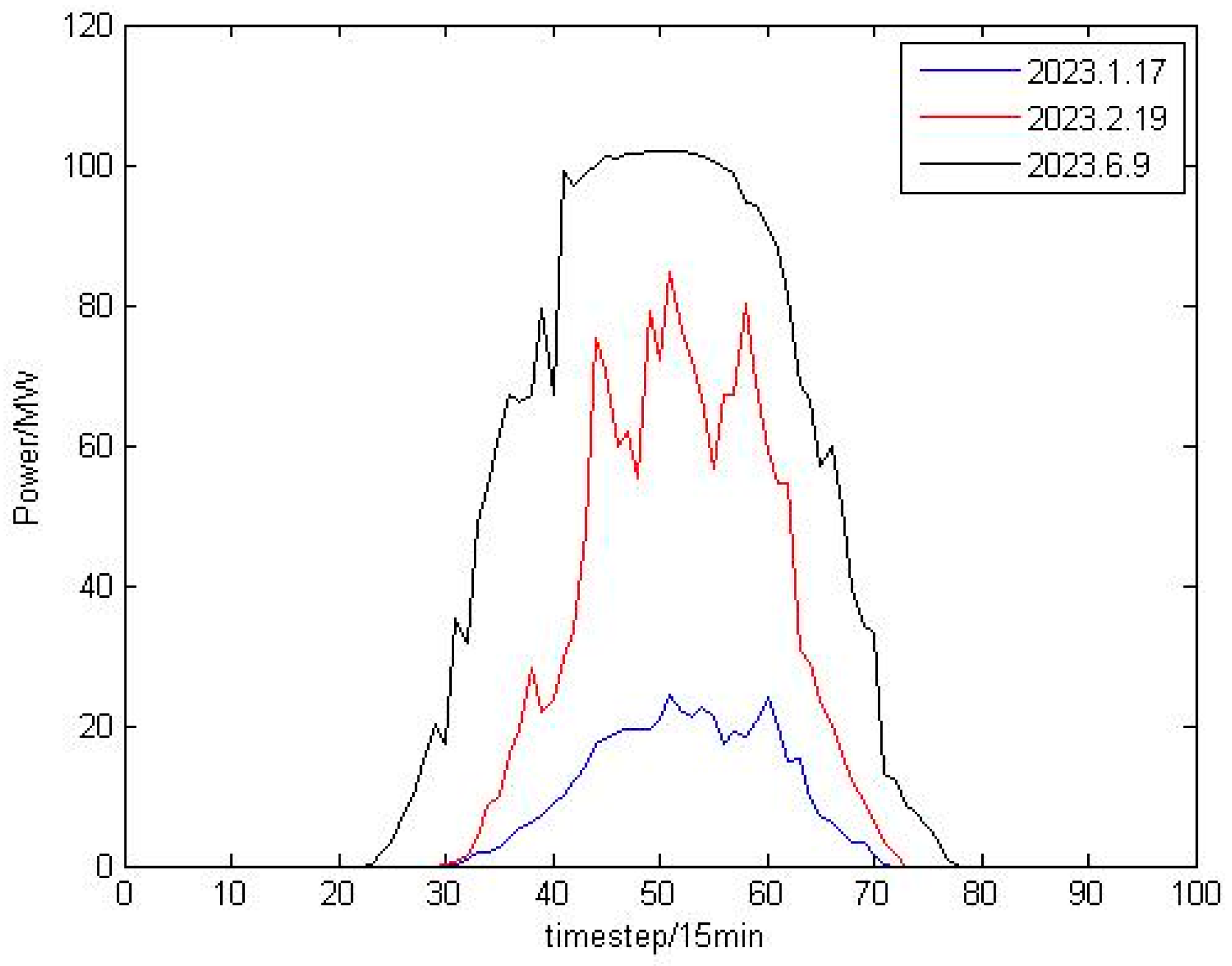
In addition, the output of photovoltaic power plants has obvious seasonal characteristics, which means that there are differences in the amplitude and trend of photovoltaic output in different seasons. Figure 2 shows three daily photovoltaic output curves for different months. From the figure, it can be seen that compared to winter, the effective time of photovoltaic output power in summer is longer, which is related to the longer duration of sunlight in summer. Specifically, the photovoltaic output value on 17 January 2023 was greater than 0 between 7:30 a.m. and 5:30 p.m., while the photovoltaic output value on 9 June 2023 was greater than 0 from 5:30 a.m. to 7:30 p.m. In addition, the amplitude of the photovoltaic output on 9 June was significantly higher than the other two days. This is because there are differences in irradiance throughout the year, with higher irradiance in summer and autumn and lower irradiance in winter; the output power of photovoltaic power generation varies significantly in different seasons.

2.2. Data Processing

From the above data analysis, it can be concluded that the photovoltaic output data have daily periodicity, seasonality characteristics, and randomness. Therefore, the STL [27] is adopted to decompose the photovoltaic output data Xt into three parts: the seasonal term St, the trend term Tt, and the residual term Rt, laying the foundation for subsequent predictions, as shown in Equation (1):
X t = S t + T t + R t
where the trend term Tt indicates the long-term trend of data changes, the seasonal term St represents periodic fluctuations, and the residual term Rt represents random fluctuations or noise components.
Specifically, a preliminary decomposition of the photovoltaic output time series is first carried out to separate the seasonal and trend components for initial estimation. Then, the local weighted regression method is used to smooth the seasonal and trend terms separately. Finally, the residual term is calculated after removing the trend and seasonal components. Moreover, the STL decomposition is an iterative process that repeatedly adjusts trends and seasonal components based on residuals until certain convergence conditions are met.
Then, to reduce the impact of dimensional differences in each component data, maximum and minimum normalization is performed on all components as follows:
x s t d = x x min x max x min
where x is the true value of each component, xmax and xmin are the maximum and minimum values of the data, respectively, and xstd is the normalized result.
In the end, the dataset of the season term is divided into the training set Trs, validation set Vas, and testing set Tes according to the a:b:c ratio. Similarly, other training sets Trt, Trr, validation set Vat, Var, and test set Tet, Ter can be obtained.

3. Method

Based on the above data analysis and processing, a short-term photovoltaic output prediction method is proposed in this section based on the neural networks. Specifically, the TCN models are built to predict the short-term photovoltaic output; on the other hand, denoising of prediction errors and establishment of error correction models can further improve prediction accuracy.

3.1. TCN Model Process

The photovoltaic output dataset has been decomposed into three sub-datasets through STL: seasonal term, trend term, and residual term. The data change patterns vary in different sub-datasets, so prediction models for different sub-datasets will be established in this section and the photovoltaic output prediction results will be obtained by superimposing the prediction results.
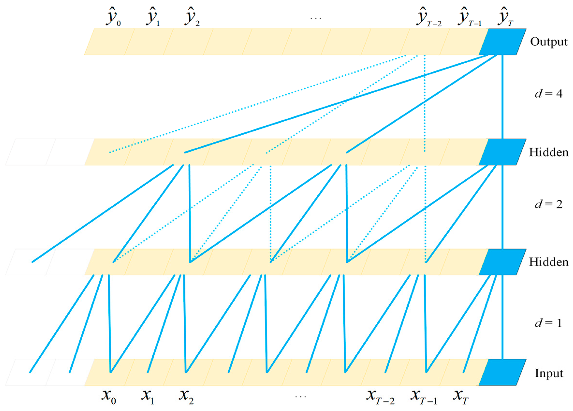
TCN is a kind of 1D fully convolutional network by combining causal convolution and dilated convolution, whose structure is shown in Figure 3 [28]. From the figure, the output at time t only depends on the input data at and before time t, which solves the problem of historical data forgetting in traditional convolution. Unlike traditional convolution, dilated convolution allows for interval sampling of the input during convolution, with the dilation rate d = 2l (l = 0, 1, 2, ……). The mathematical expression is as follows:
y ( t ) = s = 0 k 1 w ( s ) x ( t d s )
where x(t) is the input sequence, y(t) is the output of the dilation causal convolution, k is the kernel size, and w(s) is the kernel function. Therefore, dilated convolution causes the size of the effective window to increase exponentially with the number of layers. Through this method, convolutional networks can obtain a large receptive field with fewer layers. Among them, the receptive field size RFS of the L-th layer output node is as follows:
R F S = 1 + l = 0 L 1 ( k 1 ) 2 l = 1 + ( k 1 ) ( 2 L 1 )
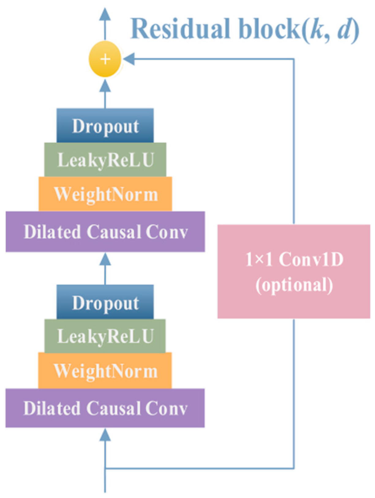
By increasing the expansion coefficient or increasing the size of the filter, the receptive field can be flexibly changed, allowing the network to fully explore the time-domain features in the data. To solve the problem of gradient vanishing in deep networks while maintaining temporal consistency between input and output, residual blocks are introduced, with the structure shown in Figure 4. Moreover, instead of the commonly used activation function ReLU, a variant of ReLU called Leaky ReLU has been proposed, and the calculation formula is as follows:
L e a k y R e L U ( x ) = x i f   x 0 a x f   x < 0
Among them, a is a small positive number, usually set to 0.01 or other values close to zero. In this way, even when the input is negative, the gradient will not completely disappear.
Therefore, considering the advantages of the TCN model in processing long time series, the prediction models based on TCN are established for various components of photovoltaic output data.

3.2. Error Correction Models

According to data analysis, photovoltaic output has randomness and volatility, especially when encountering extreme weather, which brings significant errors to the prediction. In addition, overfitting or underfitting of the prediction model can also bring errors to the prediction of the photovoltaic output. To further reduce the impact of photovoltaic uncertainty and inherent model errors on prediction accuracy, this section proposes an error correction method based on error prediction.
Considering that the error sequence fluctuates violently and does not have obvious temporal characteristics, the CEEMDAN method is used to filter and denoise the error data decomposition, separating the noise while preserving the feature information. CEEMDAN is an improvement upon empirical mode decomposition (EMD), which is mainly used for processing non-stationary time series signals [29]. CEEMDAN not only solves the problem of residual noise transferring from high-frequency components to low-frequency components during EEMD and CEEMD decomposition processes by introducing adaptive noise but also improves computational efficiency and accuracy.
Using CEEMDAN, the prediction error of photovoltaic output is decomposed, and multiple intrinsic mode function (IMF) components and a residual term are obtained from high frequency to low frequency in sequence. The expression is as follows:
e ( t ) = i = 1 k I M F i ( t ) + r e s
where e(t) indicates the prediction error sequence, IMFi(t) is the data sequence of the i-th IMF component, k denotes the total number of IMF components, and res is the residual. Due to the fact that noise mainly exists in high-frequency components, the denoised error sequence can be obtained by removing some high-frequency components and reconstructing the data. On this basis, error prediction models based on TCN are built.

3.3. Performance Evaluation

In this article, the performance evaluation indicators consist of normalized Mean Absolute Error (nMAE) [30], normalized Root Mean Square Error (nRMSE) [31], and R2 [32], which quantify the prediction error while demonstrating the fitting degree of the proposed model. The calculation formulas are as follows:
n M A E = 1 N t = 1 N y ^ t y t y m a x y m i n
n R M S E = 1 N t = 1 N y ^ t y t y max y m i n 2
R 2 = 1 t = 1 N y ^ t y t 2 t = 1 N y t y ¯ 2
where yt and y ^ t are the true and predicted values of the t-th sample, respectively; y ¯ denotes the mean value of all the samples; N is the total number of samples; and ymax and ymin are the maximum and minimum of true values, respectively.

3.4. Workflow of the Proposed Methods

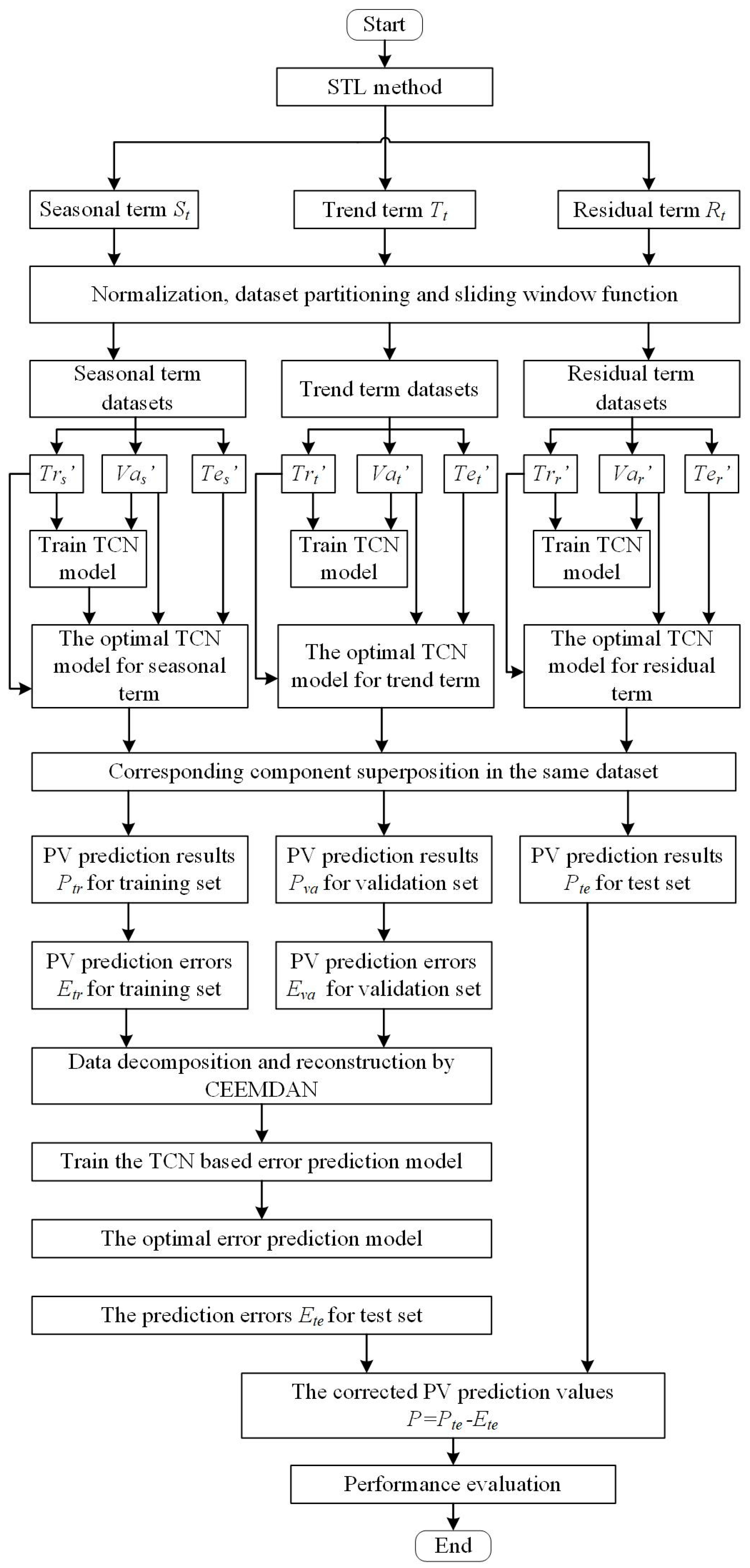
Based on the above prediction model and error correction method, this section presents the short-term photovoltaic output prediction process, as shown in Figure 5.
First, according to the input format requirements of the TCN, it is necessary to use the sliding window function to reconstruct the dataset into a three-dimensional matrix format of (m,t,p). Among them, m represents the number of samples, t represents the time step of the input sequence, and p represents the feature dimension contained at each time point of the sample. Therefore, through the sliding time window algorithm, new training sample sets Trs, Trt, Trr, validation sample sets Vas, Vat, Var, and testing sample sets Tes, Tet, Ter for each component are obtained.
Secondly, three TCN models are trained using the training sample sets Trs, Trt, Trr, and the network parameters are updated using the validation sample set data Vas, Vat, Var and the Adam algorithm. During this process, the early stopping mechanism is adopted to interrupt training and prevent overfitting. Then, all the datasets of each component are fed into the corresponding optimal networks to obtain the predicted values of the corresponding components. And the photovoltaic output prediction results Ptr, Pva, Pte will be obtained by superimposing the prediction results of the corresponding components in the same dataset.
Then, the prediction errors Etr, Eva of the training set and validation set can be obtained by subtracting the predicted values from the true values. Before building the error prediction model, use CEEMDAN to decompose and reconstruct the error data in the training and validation sets. By using the denoised error data, a TCN-based error prediction model is obtained through model training and validation. By predicting the error Ete of the test sample set data, the photovoltaic output of the test set is corrected; that is, the final photovoltaic output prediction value is the predicted value of the photovoltaic output before correction minus the prediction error. Finally, a comprehensive evaluation of the prediction model and prediction results is conducted based on the evaluation indicators.

4. Analysis of the Experiments

In order to verify the progressiveness of the photovoltaic output prediction method proposed in this paper, this section adopts the dataset in Section 2 to carry out ablation experiments and comparative experiments. The software development environment of the system is Python 3.8, and the code is written in combination with deep learning open-source frameworks Tensorflow (version 2.1.0), Pytorch (version 1.7.1), and Cuda (Version 10.2).

4.1. Experimental Process

During the experiment, in order to predict the photovoltaic output for the next hour, the photovoltaic output data from the previous 8 h are selected as the input for the model. It is worth noting that, because meteorological data and plant metadata are often unavailable in practice, this study focuses on univariate forecasting using only power data. According to the 15 min sampling period, there are 96 photovoltaic output data samples per day, and the STL period is set to 96. After data normalization, the training set is from January to April 2023, the validation set is from May 2023, and the test set is from June 2023, in a ratio of 4:1:1. Then, the new sample datasets are reconstructed through the sliding window method. Among them, the lengths of the input samples and output labels are 32 and 4, respectively, with a sliding step size of 1. Based on this, the number of samples in the training set is 10,909, and the number of samples in the validation set is 2845. Table 1 provides the detailed hyperparameters of the TCN model.
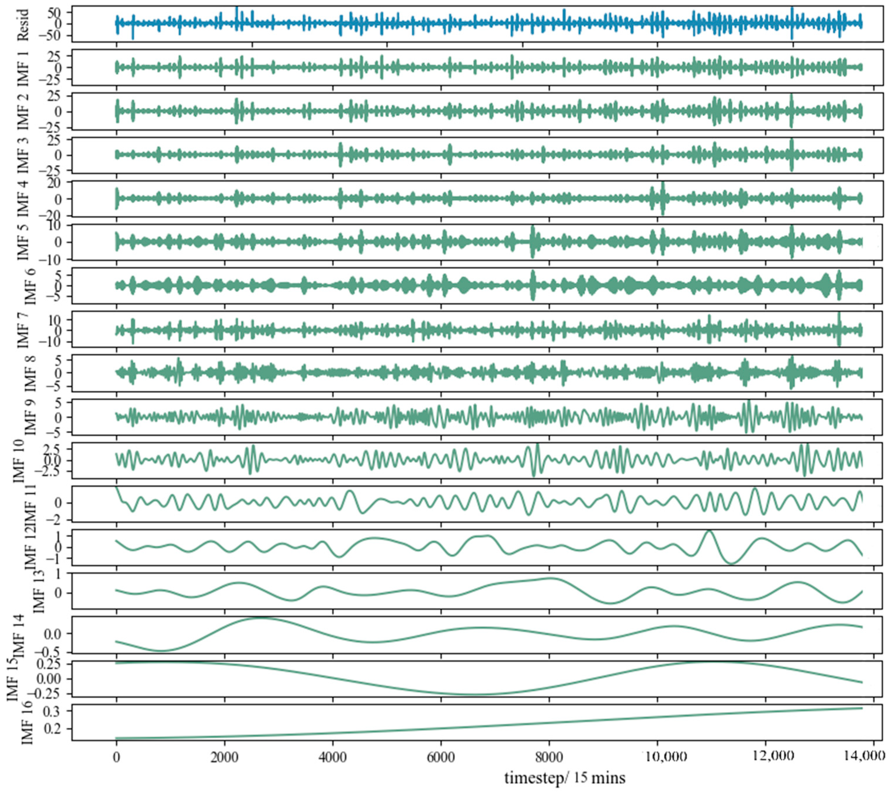
Based on the optimal TCN model, the predicted photovoltaic output values for each dataset can be achieved. At the same time, using the true values of the photovoltaic output from the training set and validation set, the obtained prediction error sequence is decomposed by CEEMDAN. The decomposition results are shown in Figure 6, which indicates that a total of 16 IMFs are obtained from high frequency to low frequency. Three high-frequency noises IMF1–3 are removed and the remaining components are superimposed to obtain a reconstructed error sequence for training an error prediction model. Then, based on the error prediction values of the photovoltaic output in the test set, the corrected photovoltaic output prediction values are achieved.

4.2. Ablation Experiments

In order to improve the prediction accuracy of the photovoltaic output, STL is adopted to decompose the photovoltaic data and then the error correction model is proposed in this paper. To verify the effectiveness of the above two improvements, this section sets up two control experiments: one group directly uses neural networks to predict photovoltaic data, the other group adopts STL to decompose the photovoltaic output first, and then neural networks are used to predict each component and obtain the final results. In addition to TCN, mainstream neural networks such as LSTM, GRU, CNN, and BP are also chosen to conduct the ablation experiments. In the experiment, the values of hyperparameters such as batch_size, epochs, learning rate, patience, dropout, dense, and loss for all neural networks are the same, as shown in Table 1. Moreover, the other hyperparameters of each model are shown in Table 2.
Randomly selecting one day in the test set, Figure 7 gives the corresponding prediction curves of these five models. Each subgraph presents three prediction curves obtained using the STL decomposition and error correction method, as well as two control experiments, under the same network model. In Figure 7a, the method proposed in this paper obtains a predicted curve that is closer to the true one compared to using TCN alone or using both TCN and STL decomposition simultaneously. Specifically, in Figure 7a, between the 48th and 59th sampling points, the true value of photovoltaic output increases from about 15 MW to 55 MW, accompanied by significant fluctuations. However, the prediction curve based on TCN cannot capture the growth trend of photovoltaic output, while the one based on STL decomposition and TCN can track the growth trend but differ significantly from the true value in terms of growth amplitude. Through further error correction process, the method proposed in this paper performs better in terms of tracking the trend and amplitude of changes in the photovoltaic output. Similarly, it can be seen from Figure 7b–e that corresponding results can also be obtained for ablation experiments on other networks.
In addition, for the various models mentioned above, the evaluation indicators for the prediction results on the entire test set are calculated. The results are shown in Table 3, where the RMSE and MAE indicators are normalized values. From the statistical data, it can be seen that for the same prediction network, performing STL decomposition on the data for prediction and error correction on the prediction results can result in smaller prediction errors and larger R2. This indicates the effectiveness and necessity of data decomposition and error correction models, although this may increase the training time and parameter count of the model. On this basis, compared with other networks, using TCN as the prediction model can further improve both the accuracy and the fitting degree; that is, the MAE and RMSE of TCN-STL-ECM are smallest and the R2 is largest.

4.3. Comparative Experiments

The above ablation experiments have verified the advantages of STL decomposition and error correction. On this basis, this subsection will conduct comparative experiments to show the advancement of the proposed method from the perspective of the prediction curve of a certain day and the prediction performance of the entire test set. Figure 8 shows the prediction curves of five methods for a certain day in the test set. It is evident that the method proposed in this paper performs the best on this sample, and the predicted curve is closest to the true one whether in terms of overall trends or local fluctuations. Specifically, between the 58th and 70th sampling points, the true curve of the photovoltaic output fluctuates. Most methods do not predict this trend, while the TCN + STL + ECM method accurately predicts the changes in the curve and achieves the minimum prediction error.
Table 4 presents the evaluation indicators for the comparative experiments of the entire test set. The normalized MAE, RMSE, and R2 of the proposed method are 0.0571, 0.0917, and 0.922, respectively. Therefore, even if prediction methods based on other networks also incorporate data decomposition and error correction, there is still a gap in performance indicators compared to the method proposed in this paper.
In conclusion, this section, on the one hand, verifies the effectiveness of data decomposition and error correction through ablation experiments, and on the other hand, verifies the progressiveness of the TCN through comparative experiments.

5. Conclusions

This paper has proposed a short-term photovoltaic prediction method based on STL decomposition and error prediction to further improve prediction accuracy. On the one hand, STL is used to decompose photovoltaic data, and at the same time, the variation characteristics of each component data are mined based on the TCN to obtain photovoltaic output prediction results. On the other hand, an error prediction model is constructed based on TCN to predict errors and achieve correction of photovoltaic predictions. In addition, various mainstream neural network models have been utilized for ablation and comparative experiments to illustrate the effectiveness and advancement of the proposed method in this paper. The photovoltaic output prediction method proposed in this paper provides a solution for practical situations where the data source is single and the prediction accuracy needs to be improved. With the diversity of data sources, we will further consider the impact of meteorological factors and related operational data.

Author Contributions

Conceptualization, C.L. and J.T.; methodology, C.L., Y.Z. and Z.Z.; software, C.L., Y.Z. and Z.Z.; validation, L.Z. and J.T.; formal analysis, Z.Z. and L.Z.; investigation, Y.Z. and Z.Z.; resources, C.L.; data curation, Y.Z. and L.Z.; writing—original draft preparation, C.L. and Y.Z.; writing—review and editing, J.T.; visualization, Y.Z. and Z.Z.; supervision, J.T.; project administration, C.L. and L.Z.; funding acquisition, C.L. and L.Z. All authors have read and agreed to the published version of the manuscript.

Funding

This research was funded by the Science and Technology Projects from State Grid Gansu Electric Power Company, grant number B3272225000P; Smart Grid-National Science and Technology Major Project, grant number 2024ZD0800500.

Informed Consent Statement

Not applicable.

Data Availability Statement

Data are available on reasonable request.

Conflicts of Interest

The authors declare no conflicts of interest.

Abbreviations

The following abbreviations are used in this manuscript:
STLSeasonal and Trend decomposition using Loess
TCNTemporal convolutional network
SVMSupport vector machine
ANNsArtificial neural networks
PSOParticle swarm optimization
BPBackpropagation
RNNRecurrent neural network
LSTMLong short-term memory
CNNConvolutional neural network
ACOAnt colony optimization
WPDWavelet packet decomposition
CEEMDANComplete ensemble empirical mode decomposition with adaptive noise
EMDEmpirical mode decomposition
MAEMean absolute error
RMSERoot mean square error

References

  1. Ahmed, R.; Sreeram, V.; Mishra, Y.; Arif, M.D. A Review and Evaluation of the State-of-the-Art in PV Solar Power Forecasting: Techniques and Optimization. Renew. Sustain. Energy Rev. 2020, 124, 109792. [Google Scholar] [CrossRef]
  2. Das, U.K.; Tey, K.S.; Seyedmahmoudian, M.; Mekhilef, S.; Idris, M.Y.I.; Van Deventer, W.; Horan, B.; Stojcevski, A. Forecasting of Photovoltaic Power Generation and Model Optimization: A Review. Renew. Sustain. Energy Rev. 2018, 81, 912–928. [Google Scholar] [CrossRef]
  3. Mayer, M.J.; Gróf, G. Extensive Comparison of Physical Models for Photovoltaic Power Forecasting. Appl. Energy 2021, 283, 116239. [Google Scholar] [CrossRef]
  4. Akhter, M.N.; Mekhilef, S.; Mokhlis, H.; Mohamed Shah, N. Review on Forecasting of Photovoltaic Power Generation Based on Machine Learning and Metaheuristic Techniques. IET Renew. Power Gener. 2019, 13, 1009–1023. [Google Scholar] [CrossRef]
  5. Böök, H.; Lindfors, A.V. Site-Specific Adjustment of a NWP-Based Photovoltaic Production Forecast. Sol. Energy 2020, 211, 779–788. [Google Scholar] [CrossRef]
  6. Larson, D.P.; Coimbra, C.F. Direct Power Output Forecasts from Remote Sensing Image Processing. J. Sol. Energy Eng. 2018, 140, 021011. [Google Scholar] [CrossRef]
  7. Pedro, H.T.; Coimbra, C.F. Assessment of Forecasting Techniques for Solar Power Production with No Exogenous Inputs. Sol. Energy 2012, 86, 2017–2028. [Google Scholar] [CrossRef]
  8. Yang, C.; Thatte, A.A.; Xie, L. Multitime-Scale Data-Driven Spatio-Temporal Forecast of Photovoltaic Generation. IEEE Trans. Sustain. Energy 2014, 6, 104–112. [Google Scholar] [CrossRef]
  9. Sheng, H.; Xiao, J.; Cheng, Y.; Ni, Q.; Wang, S. Short-Term Solar Power Forecasting Based on Weighted Gaussian Process Regression. IEEE Trans. Ind. Electron. 2017, 65, 300–308. [Google Scholar] [CrossRef]
  10. Jiang, Y.; Long, H.; Zhang, Z.; Song, Z. Day-Ahead Prediction of Bi-Hourly Solar Radiance with a Markov Switch Approach. In Proceedings of the 2018 IEEE Power & Energy Society General Meeting (PESGM), Portland, OR, USA, 5–10 August 2018; p. 1. [Google Scholar]
  11. Ding, S.; Li, R.; Tao, Z. A Novel Adaptive Discrete Grey Model with Time-Varying Parameters for Long-Term Photovoltaic Power Generation Forecasting. Energy Convers. Manag. 2021, 227, 113644. [Google Scholar] [CrossRef]
  12. Eseye, A.T.; Zhang, J.; Zheng, D. Short-Term Photovoltaic Solar Power Forecasting Using a Hybrid Wavelet-PSO-SVM Model Based on SCADA and Meteorological Information. Renew. Energy 2018, 118, 357–367. [Google Scholar] [CrossRef]
  13. Das, U.K.; Tey, K.S.; Seyedmahmoudian, M.; Idna Idris, M.Y.; Mekhilef, S.; Horan, B.; Stojcevski, A. SVR-Based Model to Forecast PV Power Generation under Different Weather Conditions. Energies 2017, 10, 876. [Google Scholar] [CrossRef]
  14. de Paiva, G.M.; Pimentel, S.P.; Marra, E.G.; de Alvarenga, B.P.; Mussetta, M.; Leva, S. Intra-Day Forecasting of Building-Integrated PV Systems for Power Systems Operation Using ANN Ensemble. In Proceedings of the 2019 IEEE Milan PowerTech, Milan, Italy, 23–27 June 2019; pp. 1–5. [Google Scholar]
  15. Liu, J.; Fang, W.; Zhang, X.; Yang, C. An Improved Photovoltaic Power Forecasting Model with the Assistance of Aerosol Index Data. IEEE Trans. Sustain. Energy 2015, 6, 434–442. [Google Scholar] [CrossRef]
  16. Mahmud, K.; Azam, S.; Karim, A.; Zobaed, S.; Shanmugam, B.; Mathur, D. Machine Learning Based PV Power Generation Forecasting in Alice Springs. IEEE Access 2021, 9, 46117–46128. [Google Scholar] [CrossRef]
  17. Wang, G.; Yang, M.; Yu, Y. A Short-Term Forecasting Method for Photovoltaic Power Based on Ensemble Adaptive Boosting Random Forests. In Proceedings of the 2020 IEEE/IAS 56th Industrial and Commercial Power Systems Technical Conference, Las Vegas, NV, USA, 29 June–28 July 2020; pp. 1–8. [Google Scholar]
  18. Li, G.; Wang, H.; Zhang, S.; Xin, J.; Liu, H. Recurrent Neural Networks Based Photovoltaic Power Forecasting Approach. Energies 2019, 12, 2538. [Google Scholar] [CrossRef]
  19. Garip, Z.; Ekinci, E.; Alan, A. Day-Ahead Solar Photovoltaic Energy Forecasting Based on Weather Data Using LSTM Networks: A Comparative Study for Photovoltaic (PV) Panels in Turkey. Electr. Eng. 2023, 105, 3329–3345. [Google Scholar] [CrossRef]
  20. Agga, A.; Abbou, A.; Labbadi, M.; El Houm, Y.; Ali, I.H.O. CNN-LSTM: An Efficient Hybrid Deep Learning Architecture for Predicting Short-Term Photovoltaic Power Production. Electr. Power Syst. Res. 2022, 208, 107908. [Google Scholar] [CrossRef]
  21. Wang, K.; Qi, X.; Liu, H. Photovoltaic Power Forecasting Based LSTM-Convolutional Network. Energy 2019, 189, 116225. [Google Scholar] [CrossRef]
  22. Souhe, F.G.Y.; Mbey, C.F.; Kakeu, V.J.F.; Meyo, A.E.; Boum, A.T. Optimized Forecasting of Photovoltaic Power Generation Using Hybrid Deep Learning Model Based on GRU and SVM. Electr. Eng. 2024, 106, 7879–7898. [Google Scholar] [CrossRef]
  23. Li, P.; Zhou, K.; Lu, X.; Yang, S. A Hybrid Deep Learning Model for Short-Term PV Power Forecasting. Appl. Energy 2020, 259, 114216. [Google Scholar] [CrossRef]
  24. Chen, J.; Peng, T.; Qian, S.; Ge, Y.; Wang, Z.; Nazir, M.S.; Zhang, C. An Error-Corrected Deep Autoformer Model via Bayesian Optimization Algorithm and Secondary Decomposition for Photovoltaic Power Prediction. Appl. Energy 2025, 377, 124738. [Google Scholar] [CrossRef]
  25. Tao, K.; Zhao, J.; Tao, Y.; Qi, Q.; Tian, Y. Operational Day-Ahead Photovoltaic Power Forecasting Based on Transformer Variant. Appl. Energy 2024, 373, 123825. [Google Scholar] [CrossRef]
  26. Zhou, D.; Liu, Y.; Wang, X.; Wang, F.; Jia, Y. Combined Ultra-Short-Term Photovoltaic Power Prediction Based on CEEMDAN Decomposition and RIME Optimized AM-TCN-BiLSTM. Energy 2025, 318, 134847. [Google Scholar] [CrossRef]
  27. Cleveland, R.B.; Cleveland, W.S. STL: A Seasonal-Trend Decomposition Procedure Based on Loess. J. Off. Stat. 1990, 6, 3–73. [Google Scholar]
  28. Bai, S.; Kolter, J.Z.; Koltun, V. An Empirical Evaluation of Generic Convolutional and Recurrent Networks for Sequence Modeling. arXiv 2018, arXiv:1803.01271. [Google Scholar] [CrossRef]
  29. Torres, M.E.; Colominas, M.A.; Schlotthauer, G.; Flandrin, P. A Complete Ensemble Empirical Mode Decomposition with Adaptive Noise. In Proceedings of the 2011 IEEE International Conference on Acoustics, Speech and Signal Processing, Prague, Czech Republic, 22–27 May 2011; pp. 4144–4147. [Google Scholar]
  30. Krevnevičiūtė, J.; Mitkevičius, A.; Naujokaitis, D.; Lagzdinytė-Budnikė, I.; Marčiukaitis, M. The Forecast of the Wind Turbine Generated Power Using Hybrid (LTC + XGBoost) Model. Appl. Sci. 2025, 15, 7615. [Google Scholar] [CrossRef]
  31. Xu, M.; Zhu, R.; Yu, C.; Mi, X. DHGAR: Multi-Variable-Driven Wind Power Prediction Model Based on Dynamic Heterogeneous Graph Attention Recurrent Network. Appl. Sci. 2025, 15, 1862. [Google Scholar] [CrossRef]
  32. Birkelund, Y. Numerical Weather Modelling and Large Eddy Simulations of Strong-Wind Events in Coastal Mountainous Terrain. Appl. Sci. 2025, 15, 7683. [Google Scholar] [CrossRef]
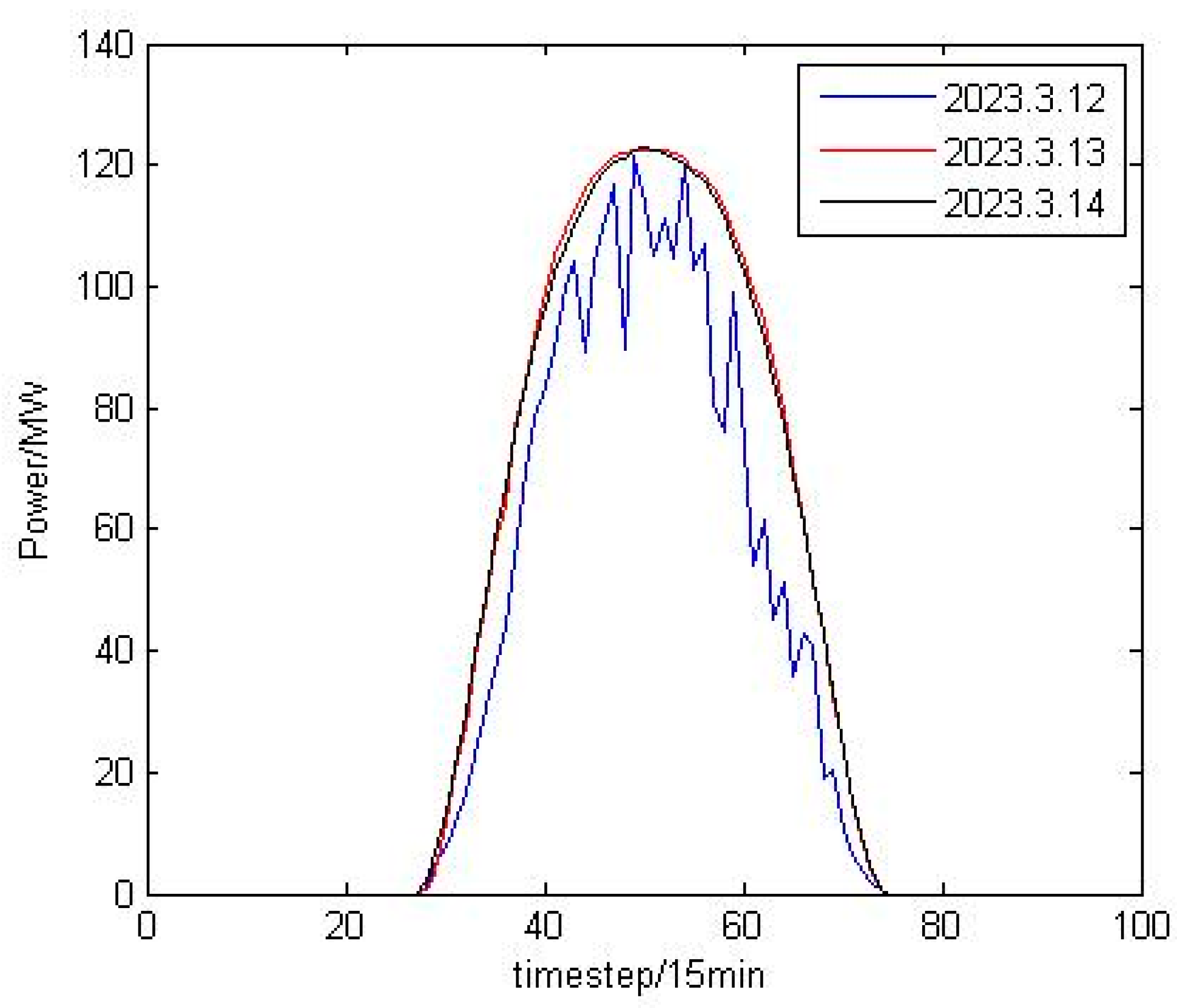
Figure 1. The daily photovoltaic output curves from 11 to 13 January 2023.
Applsci 15 11089 g001
Figure 2. Three daily photovoltaic output curves for different months.
Applsci 15 11089 g002
Figure 3. Structure diagram of dilated causal convolution.
Applsci 15 11089 g003
Figure 4. Schematic diagram of residual block.
Applsci 15 11089 g004
Figure 5. Flowchart of the short-term photovoltaic output prediction method.
Applsci 15 11089 g005
Figure 6. The decomposition results of CEEMDAN for prediction error sequences.
Applsci 15 11089 g006
Figure 7. Prediction curves of different models for a certain day in the test set: (a) TCN; (b) GRU; (c) LSTM; (d) CNN; (e) BPNN.
Applsci 15 11089 g007
Figure 8. Prediction curves of five methods for a certain day in the test set.
Applsci 15 11089 g008
Table 1. Hyperparameters of TCN model.
HyperparametersValues
batch_size16
epochs100
learning rate0.001
patience10
Dropout0.1
Dense4
LossMSE
filter_nums12
kernel_size8
nb_stacks2
Table 2. Other hyperparameters of each model.
ModelHyperparameterValue
LSTMunits12, 10, 8
GRUunits16, 12, 8
CNNfilters16, 10, 8
BPNNdense16, 12, 8
Table 3. Performance indicators of prediction results using different methods.
MethodnMAEnRMSER2Training TimeParams
TCN0.07320.19400.854163.1329,164
TCN + STL0.05990.09910.884888.8929,164
TCN + STL + ECM0.05710.09170.922484.4159,684
LSTM0.16750.18830.867138.862236
LSTM + STL0.19230.18420.883516.332236
LSTM + STL + ECM0.06320.08880.91297.772236
GRU0.09650.18420.871157.892556
GRU + STL0.08970.11160.876561.972556
GRU + STL + ECM0.05940.10810.907287.462556
CNN0.19580.28370.85728.741242
CNN + STL0.18020.20970.870124.991242
CNN + STL + ECM0.14120.16270.91029.951242
BPNN0.18020.28530.87412.32872
BPNN + STL0.17300.18260.88146.72872
BPNN + STL + ECM0.14360.13820.91326.50872
Table 4. Performance indicators for the comparative experiments of the entire test set.
MethodnMAEnRMSER2
TCN + STL + ECM0.05710.09170.922
LSTM + STL + ECM0.06320.08880.912
GRU + STL + ECM0.05940.10810.907
CNN + STL + ECM0.14120.16270.910
BPNN + STL + ECM0.14360.13820.913
Disclaimer/Publisher’s Note: The statements, opinions and data contained in all publications are solely those of the individual author(s) and contributor(s) and not of MDPI and/or the editor(s). MDPI and/or the editor(s) disclaim responsibility for any injury to people or property resulting from any ideas, methods, instructions or products referred to in the content.